Short-Term X-ray Variability during Different Activity Phases of Blazars S5 0716+714 and PKS 2155-304


1
Aryabhatta Research Institute of Observational Sciences (ARIES), Manora Peak, Nainital 263001, India
2
Centre for Theoretical Physics, Jamia Millia Islamia, New Delhi 110025, India
*
Author to whom correspondence should be addressed.
†
Aryabhatta Postdoctoral Fellow.
Galaxies 2020, 8(3), 66; https://0-doi-org.brum.beds.ac.uk/10.3390/galaxies8030066
Submission received: 4 August 2020
/
Revised: 1 September 2020
/
Accepted: 3 September 2020
/
Published: 6 September 2020
(This article belongs to the Special Issue X-Ray Flux and Spectral Variability of Blazars)
Abstract
:We explored the statistical properties of short-term X-ray variability using long-exposure XMM-Newton data during high X-ray variability phases of blazars S5 0716+714 and PKS 2155-304. In general, the hardness ratio shows correlated variations with the source flux state (count rate), but in a few cases, mainly the bright phases, the trend is complex with both correlation and anti-correlation, indicating spectral evolution. Stationarity tests suggest the time series are non-stationarity or have trend stationarity. Except for one, none of the histogram fits resulted in a reduced- for a normal and log-normal profile but a normal profile is favored in general. On the contrary, the Anderson–Darling test favors log-normal with a test-statistic value lower for log-normal over normal for all the observations, even if out of significance limits. None of the IDs show linear RMS-flux relation. The contrary inferences from different widely used statistical methods indicate that a careful analysis is needed while the complex behavior of count rate with hardness ratio suggests spectral evolution over a few 10 s of kilo-seconds during bright phases of the sources. In these cases, the spectrum extracted from whole observation may not be meaningful for spectral studies and certainly not a true representation of the spectral state of the source.
1. Introduction
Strong and rapid variability has been one of the defining criteria of blazars—active galactic nuclei with a powerful relativistic jet of plasma directed within a few degrees with our line of sight. Studies focusing on temporal flux variability have found them to be variable on all timescales accessible to us—from the shortest allowed by the observing facilities to the longest allowed by the archived data (e.g., [1]). Though the processes responsible for the observed behavior are still unclear except for a general understanding, studies of these observations have revealed some features that have resulted in empirical classification schemes to classify and identify astrophysical objects. In the blazar parlance, the observed variability on all timescales probed so far are now widely referred into three categories: intra-day variability IDV [2]—variability within a day; short-term variability (STV)—variability on days to months; and long-term variability (LTV)—variability over a few months and longer. Among these, IDV is now one of the main tools used to identify an extra-galactic source as a blazar. A spectacular prime example of this in recent times has been in establishing a subset of narrow-line Seyfert galaxies (NLS) as blazars [3,4].
Earlier and even now, optical bands have been primarily leading the IDV studies as photon statistic at higher energies has prohibited such studies in the past. However, with the continuous advancement in detector technologies, such sub-day studies have now been possible at X-ray, (e.g., [5,6,7,8]), gamma-ray, (e.g., [9,10]), and very high energies VHEs [11,12], albeit still for bright flares. These studies have also reported sub-hours to a few minutes variability—implying a compact, highly luminous emission region, still optically thin to pair production. Combined with multi-wavelength (MW) observations on similar time scales, these studies have been invaluable in providing insights on the nature of variability and the underlying physical processes.
Variability reflects a change in the dynamical state of the system responsible for the observable and thus, offers direct access to scales and dynamics of the system except that in non-linear systems, a one-to-one relation between the observable and underlying dynamics is not clear apparently, (e.g., [13]). Similar problems exist for statistical exploration—widely different systems with almost no common physical connection can exhibit similar statistical behavior, (e.g., [14,15]). However, based on inferences/understanding from previous studies, a combination of both can be used to explore specific aspects of different problems that may offer new insights.
A major challenge in exploring blazar variability has been the enormous range of time scales involved and irregular gaps in the data which is inevitable in astronomy. Due to this, the statistical properties of blazars’ MW emission have not been explored widely until very recently. The renewed focus and targeted campaigns of blazars with good cadence observations, especially after the launch of the Fermi observatory that continuously surveys the sky at MeV–GeV energies have made such studies now possible, over both long and short timescales, (e.g., [1,16]). Attempts have been made to connect the short- and long-term behavior, (e.g., [8,17]) and compare these properties to those of other AGNs. Though they can provide a general idea, inferring any time scale by comparing long- and short-term trends are fraught with uncertainties as the short-term behavior is not yet widely established. Different studies exploring short-term behaviors have reported significant changes in these properties [5,6] over different time scales. Further, irregular gaps and statistical properties of time series e.g., stationarity, limit the use of Fourier-based methods and reliability of inferences derived from it, (e.g., [1]).
The short-term variability being primarily a result of competition between particle acceleration and cooling provides not only a key to study these two but the statistical behavior can be used to test a few models of blazars as well a comparative study with the well-established properties of AGNs. In this sense, long-term properties of variability have been explored fairly well, (e.g., [1,16,18,19,20,21]) but the short-term detailed studies are still few, (e.g., [5,6,8,22,23]), especially at high energies due to fewer long exposure observations during such occurrences. Interestingly, literature refers to blazars as extreme AGNs with emission dominated almost entirely by the relativistic jet, in stark contrast with a majority of AGNs. Yet, in the terms of statistical properties of variability, they appear similar to other AGNs—stochastic variability with a statistical trend similar to those exhibited by the accretion-powered sources in general ([19,20], and references therein). This has ignited the study of disk-jet connection in blazars as a multiplicative combination of fluctuations in the accretion-disk has been one of the widely accepted explanations for such behavior in AGNs (and accretion-powered sources in general; e.g., [24,25]). However, recently, based on simulations and the fact that blazar jets are highly magnetized, additive model like minijets-in-a-jet [26] has been found to exhibit these characteristics. The statistical behavior in this model changes drastically depending on the number of regions contributing to the emission. Studies over short duration during high variability phases can be used to test this model and also explore/establish general behaviors.
In this work, we explore the statistical properties of X-ray variability over a scale of a few minutes to days, during the highly variable episodes of blazar S5 0716+714 and PKS 2155-304. The next section presents the details of data acquisition, reduction procedures, and the selection of the sources followed by our analyses and results in Section 3. We discuss our findings, its implications, and the conclusion in Section 4.
2. Xmm-Newton X-ray Data
As our focus is investigations of statistical properties over short time scales (a few minutes to hours), the observations chosen are biased in the sense that only long exposure observations with good photon counts and exhibiting variability has been used. A high photon count rate and long exposure allow binning that results in more data points needed for statistical studies when the source has shown variability. Table 1 lists the sources and the observations used in this work. All the observations are taken from the public archive of the XMM-Newton observatory.
Reduction: We used the XMM-Newton Science Analysis System (SAS) version 15.0.0 and followed the standard data reduction procedure for the light curve extraction and analysis as described in the “XMM-Newton ABC Guide”. Firstly, for each ID, we generated a summary of the Observation Data File (ODF) and calibration index file (CIF) using the latest calibration data files. We then used the epproc tool to reprocess the data from the European Photon Imaging Camera-PN detector as it has a large collecting area in small window mode. We investigated the background light curve in the 10–12 keV band to find intervals affected by particle/solar flares. Subsequently, such intervals were removed from the data to get good time intervals (GTIs). We selected single and double events to mitigate the pile-up issue and we checked this problem by using the EPATPLOT tool. Except the ID 0124930301, none showed any significant pile-up. We removed a circular core of radius 7 arcsec to minimize the pile-up events in this particular observation ID. We then generated clean event files and the resulting GTIs are shown in Table 1. To extract the source light curve, we used a circular region of radius between 40–45 arcsec centered at the source coordinates. For background, we used circular regions with radius in the range of 40–45 arcsec, well away from the source and any bright spot on the CCD.
To generate light curves, we used the HEASARC tool XSELECT on the clean event files and selected the source and background region. We derived light curves in three energy bands: 0.3–2 keV, 2–10 keV, and 0.3–10 keV bands. The background-subtracted source light curves were extracted using the ftool task lcmath. We also used the ftool task lcurve to derive the hardness ratio (HR) between the 0.3–2 keV and 2–10 keV energy bands.
3. Analysis and Results
3.1. Light Curves
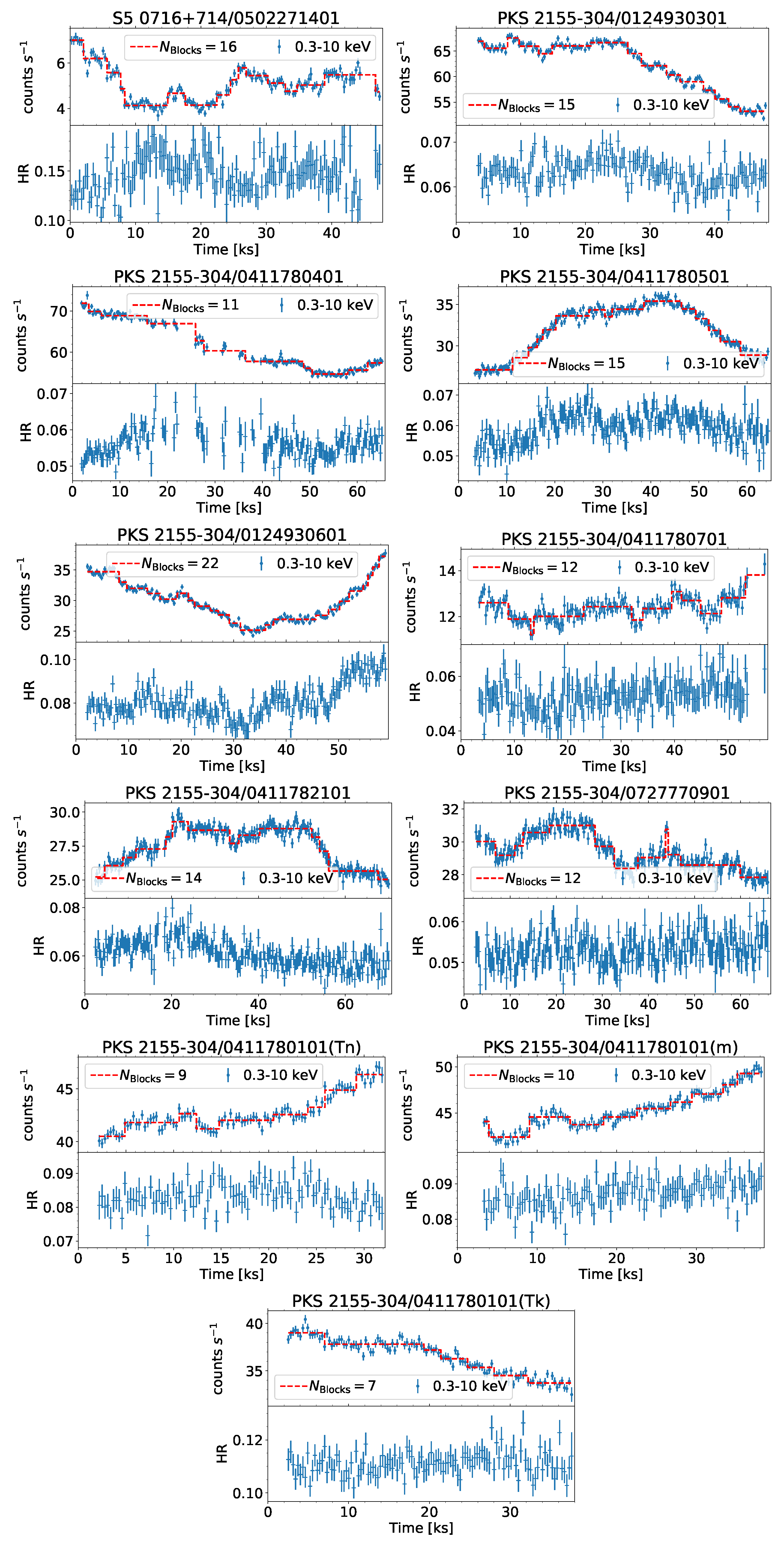
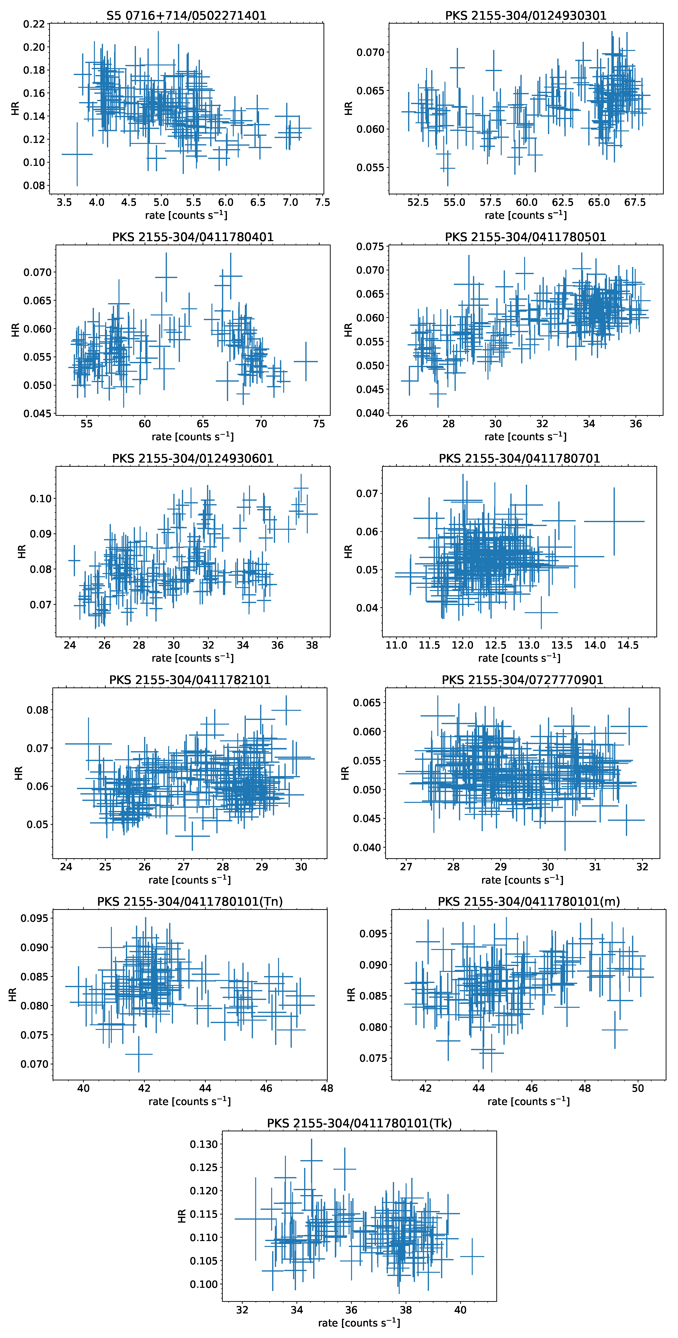
The 300 s binned light curves along with the corresponding HR for each ID as mentioned in Table 1 are shown in Figure 1. The HR here is defined as the ratio of count rate in the hard energy band i.e., 2–10 keV to the count rate in the soft energy band i.e., 0.3–2 keV. Additionally, we have shown the Bayesian blocks [27], marking significant changes in the count rate evolution with time corresponding to p = 0.075. As already stated above, the 300 s binning is employed so that we have enough data for statistical purposes and yet the discernible trends or correlations appear in light curves binned over a larger duration, e.g., 1000 s. Figure 2 shows HR as a function of the count rate in the 0.3–10 keV band.
Except for the only ID corresponding to the IBL S5 0716+714, the rest of the light curves shown in Figure 1 belong to PKS 2155-304 and capture X-ray state from very low—characterized by low count rate to a high state with a rate more than five times higher. The change in count rate is also different during different states and ranges between 1.2–1.5 (see also Figure 3 and Figure 4). Further, except for the three IDs: 0411780301, 0411780401, and 0411780101(Tn) of PKS 2155-304, the rest of the IDs show correlated variability of the count rate with HR—increase in count rate accompanied by an increase of HR and vice-versa. These three, on the other hand, show complex behavior with respect to HR. For some periods, the count rate and HR are correlated while anti-correlated—high count rate but low HR and vice-versa—for other periods. This feature is also visible in the HR plot for these IDs shown in Figure 2. It should, however, be noted that the sample size is biased, as already mentioned previously that we are interested in observations exhibiting variability and have good photon statistics. Interestingly, of these three IDs showing complex trends, the first two (0411780301, 0411780401) are the brightest of the current sample.
For S5 0716+714, we have only one observation corresponding to a high state of the source and shows count rate changes almost by a factor of two and it anti-correlates with HR.
In Table 2, we show the result of the test of stationarity using the Augmented Dickey–Fuller (ADF) test and the Kwiatkowski–Phillips–Schmidt–Shin (KPSS) test. The parenthesis marks the result for the light curve in logarithm units. Both methods check for “unit root” in the time series. The former checks for a “unit root” and difference stationarity in the time series with the null hypothesis that “a unit root exist” i.e., series is non-stationary. The latter i.e., the KPSS test, on the other hand, checks for stationarity around a deterministic trend but its null hypothesis is the opposite of the ADF i.e., the series is stationary. For both the tests, was chosen to reject the null hypothesis. Thus, in the case of ADF, rejection of the null hypothesis means that the time series is stationary while for KPSS it means a non-stationary time series.
3.2. Histogram
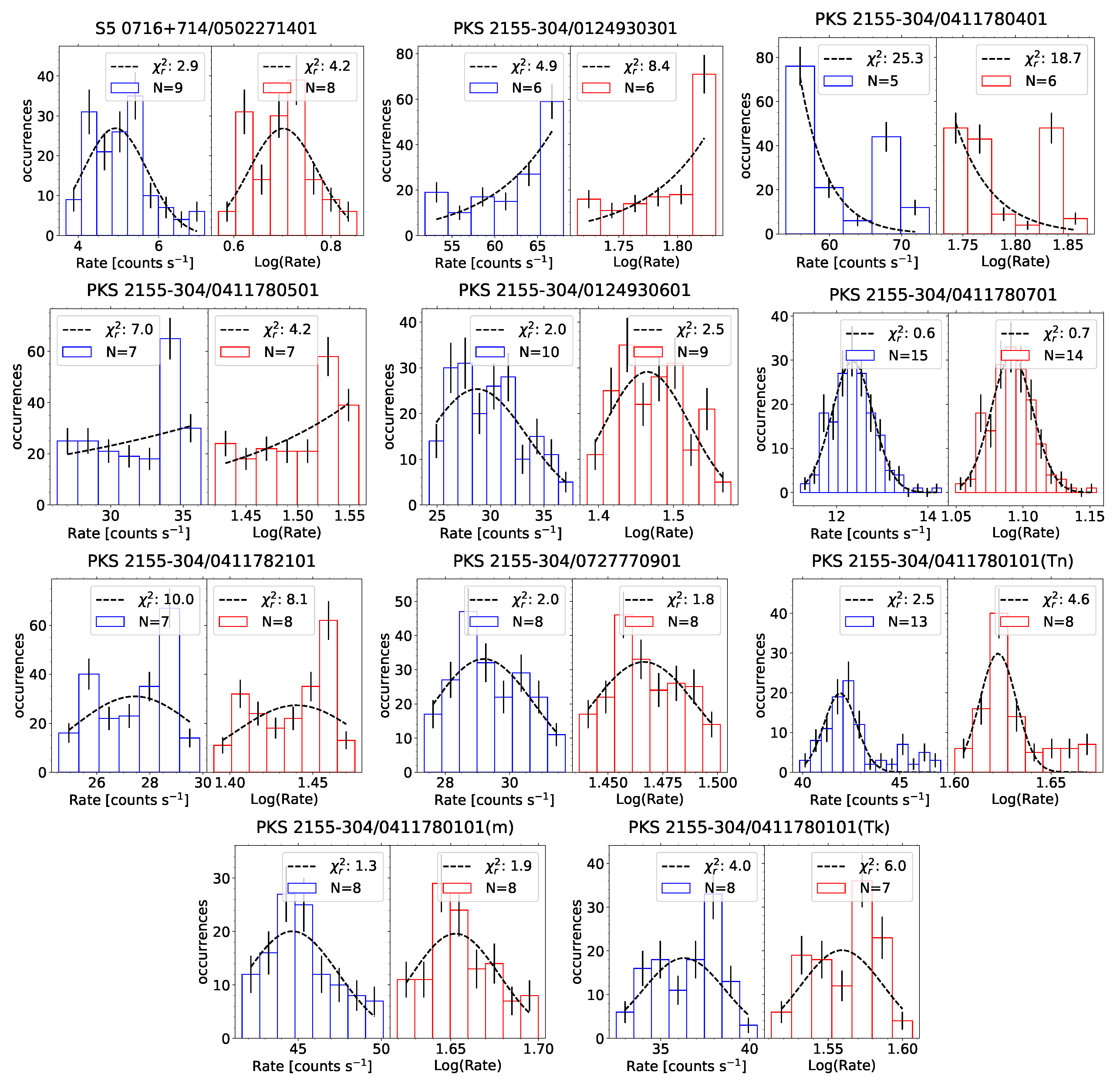
A histogram is one of the ways to visualize variations, its extent, and explore any trend/scales as well as understand the nature of variability regardless of time. Motivated by theoretical considerations and observational finding of blazars flux variation being log-normal, (e.g., [19,20]), we derived two different histograms—one from the 0.3–10 keV count rate and the other from the logarithm (unless stated otherwise, logarithm (log) throughout this work means log to the base 10) of this count rate using the Knuth method [28]. Figure 3 shows the two histograms for each ID and a Normal fit to these histograms along with the reduced- () values.
Interestingly, if we choose the lowest as one representing the data better, a Normal fit is better compared to a log-Normal for both the sources except for the three IDs—0411780501, 0411782101, and 0727770901 of PKS 2155-304. For 0411780501, the histogram rather appears more consistent with a constant while for 0727770901, log-normal is marginally better. For 0124930301 and 0411780401, even though normal is favored, the inferences are unphysical as the peak rate returned by the fit is way higher than anything reported in the literature so far.
We, additionally, also performed the Anderson–Darling (AD) test to see which of the two histograms: normal or log-normal is a better representation of the data. The result of the AD test is listed in the last column of Table 2. Interestingly, the AD test always favored a log-normal over normal whether or not the test statistic is within the critical significance level values. Further, the test values for log-Normal was consistently lower than the test values for a Normal. The ‘-’ in Table 2 means that the test result was greater than the critical value corresponding to p=0.01. These inferences are contrary to the one inferred from fitting.
3.3. Rms-Flux Relation
Photon counting being Poissonion in nature, has inherent variation. Whether the observed variability is due to this statistical fluke or real—intrinsic to the source is normally estimated by measuring variance. If the variance of the data is larger than the mean-error-squared, then the source is variable and the variability could be intrinsic to the source.
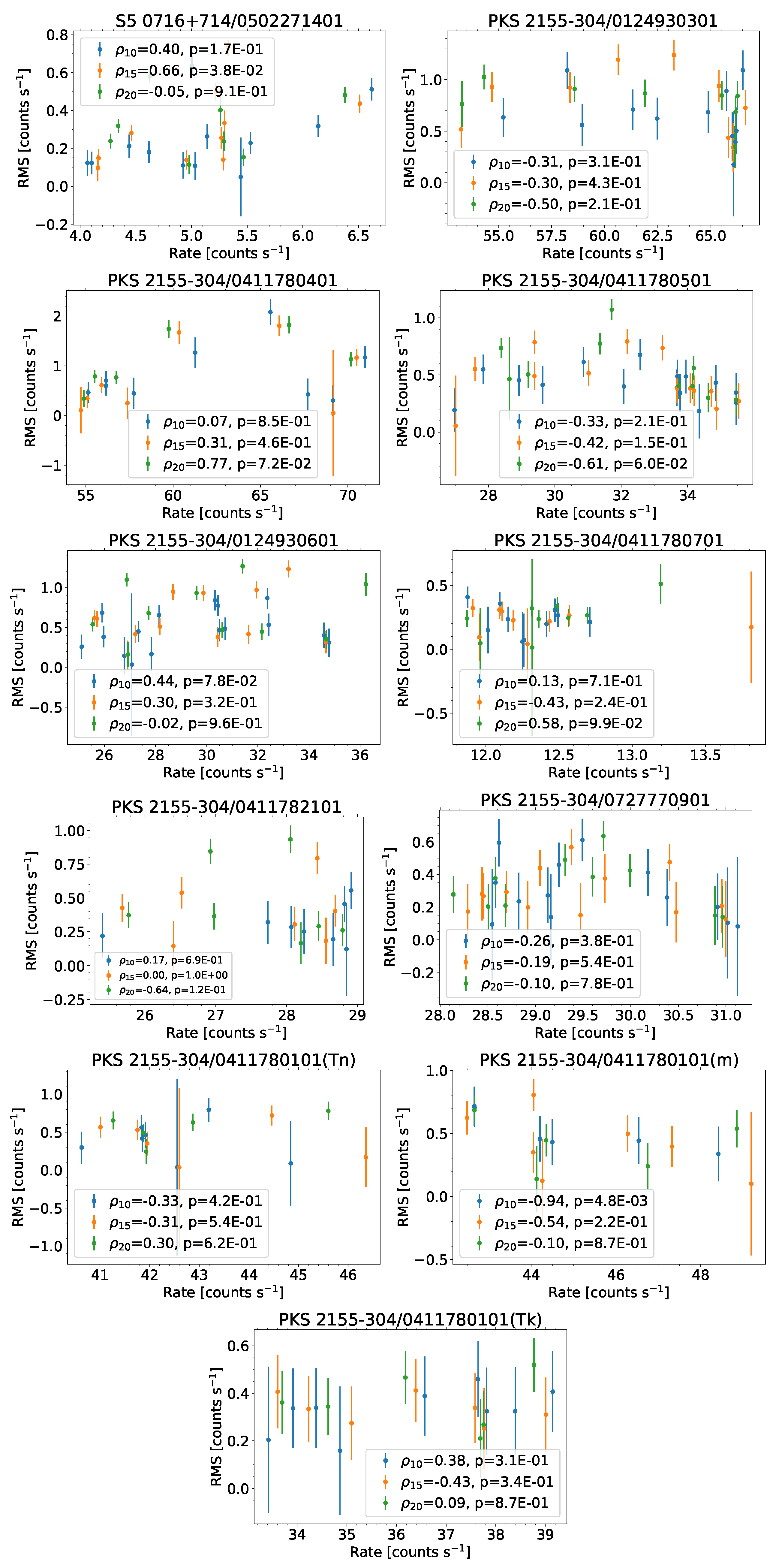
An important characteristic of accretion-powered sources and even blazars has been the linear relationship between flux/count rate and RMS (root-mean-squared) variation [5,20,29]. However, recent observations have reported a few contrary results as well ([15] and references therein). Figure 4 shows the RMS-flux relation for the current sample using 10, 15, and 20 data points per bin along with the corresponding Spearman correlation coefficient and p-value (p < 0.01 means significant correlation or anti-correlation depending on the sign of ). We also verified the RMS-flux relation using more data points per bin (e.g., 25, 30) and the outcome remains similar. None of these show any significant correlation between RMS and count rate. It should be noted that, during the calculation, a few of the segments had negative variances due to measurement error dominating the variations. We simply rejected variance in these cases.
4. Discussion and Conclusions
In this work, we explored the statistical properties of short-term (300 s binned) X-ray variability of blazar S5 0716+714 and PKS 2155-304 during high variability phases using long-exposure XMM-Newton EPIC-PN camera observations. The only ID of S5 7016+714 shows about a factor of two change in the count rate while the rest of the IDs belongs to PKS 2155-304 and represents different intensity and variability states of the source. For the later, the count rate changes by a factor of 1.2–1.5 within each ID but the intensity states covered by these IDs correspond up to a factor of 6.5. Test of stationarity using ADF and KPSS shows that the variability is highly non-stationary both in normal and logarithmic space (see Table 2) except probably for S5 0716+714 where the KPSS test suggests trend-stationarity. In fact, short-term X-ray variability of blazars has been normally found to be non-stationarity, (e.g., [5,6,8]). This suggests that using Fourier methods to investigate variability can result in erroneous inferences. However, the difference light curve derived by subtracting the previous value from the next makes all the light curves stationary except IDs 0411780501 and 0411780601 of PKS 2155-304, indicating the auto-regressive integrated moving average (ARIMA) method for timing studies as more appropriate (e.g., [8]).
In high states of the source, the observations show a complex temporal evolution of intensity vis-a-vis HR (see Figure 1). S5 0716+714 shows anti-correlation between count rate evolution with HR while for PKS 2155-304, the behavior is more complex and involved. At low to moderate count rates (≲50), count rate correlates with HR except for the thin filter observation in 0411780101 where, towards the end, HR anti-correlates with count rate. For the brightest two, the evolution is complex with correlation and anti-correlation both, indicating spectral evolution over time scales of a few 10 s of ks. Such strong X-ray spectral evolution has been seen over similar and much smaller time scales in Mrk 401, (e.g., [6]) and indicates that X-ray SED derived using full observation is not a true representative of the spectral state of the source but rather an average one [30]. In general, anti-correlation indicates a steepening of the X-ray spectrum, suggesting radiative cooling dominated evolution while correlation suggests activity driven by injection or particle acceleration, (e.g., [10]). However, the latter can also be due to additional emission regions contributing to the emission as has been argued in the case of spectral changes in Mrk 421, (e.g., [6]).
An interesting statistical property of AGNs X-ray variability has been a log-normal flux distribution and a linear relation between variance and flux. Similar behavior has been reported for blazar emission as well, both on long- and short-term observations, (e.g., [19,20,31,32]). Here, except for the one ID (0411780701) of PKS 2155-304, none of the histograms are consistent with either normal or lognormal distribution based on the method. In fact, the histograms show diverse profiles with normal distribution returning systematically lower statistic value than a log-normal, indicating a preference for normal. On the contrary, the AD test (see Table 2) always favors a log-normal with a test-statistic lower than that for a normal, regardless of whether the outcome is significant or not. Based on the AD test, three observations were found to be consistent with lognormal or both (p-value ). Similarly, none of the observations show any significant linear correlation between the count rate and excess variance (see Figure 4) except the case of medium filter observation of ID 0411780101 with 10 data points per bin. In short, data considered here neither show log-normal intensity distribution nor a linear correlation between excess variance and intensity.
Based on simulations and the fact that blazar jets are highly magnetized system, magnetic reconnection has been favored as a potential mechanism for rapid and luminous flares, (e.g., [33]). One of the statistical models based on magnetic reconnection called minijets-in-a-jet [26] predicts diverse histogram profiles, ranging from a power-law to one consistent with a log-normal depending on the number of emission regions contributing to the emission. However, the RMS-flux relation is always linear. Our results here disfavor such a model. Nonetheless, the difference in long- and short-term statistical behavior is very different and intriguing. Whether incorporating cooling and/or acceleration/injection can result in such changes remains to be seen.
Author Contributions
P.K. planned, perfomed the data analysis, and wrote the whole manuscript. M.P. performed and wrote the data reduction. All authors have read and agreed to the published version of the manuscript.
Funding
P.K. acknowledge funding from ARIES Aryabhatta Postdoctoral fellowship (AO/A-PDF/770). M.P. thanks the financial support of UGC, India program through DSKPDF fellowship (grant No. BSR/2017-2018/PH/0111).
Acknowledgments
The authors thank the anonymous referees for constructive comments and suggestions. This research has made use of archival data of XMM-Newton observatory, an ESA science mission directly funded by ESA Member States and NASA by the NASA Goddard Space Flight Center (GSFC).
Conflicts of Interest
The authors declare no conflict of interest.
Abbreviations
The following abbreviations are used in this manuscript:
| KPSS | Kwiatkowski–Phillips–Schmidt–Shin |
| ADF | Augumented Dickey–Fuller |
| AGNs | Active Galactic Nuclei |
| IDV | Intra-day variability |
| LTV | Long-term variability |
| STV | Short-term variability |
| AD | Anderson–Darling |
| HR | Hardness ratio |
References
- Goyal, A.; Stawarz, Ł.; Zola, S.; Marchenko, V.; Soida, M.; Nilsson, K.; Ciprini, S.; Baran, A.; Ostrowski, M.; Wiita, P.J.; et al. Stochastic Modeling of Multiwavelength Variability of the Classical BL Lac Object OJ 287 on Timescales Ranging from Decades to Hours. Astrophys. J. 2018, 863, 175. [Google Scholar] [CrossRef] [Green Version]
- Wagner, S.J.; Witzel, A. Intraday Variability In Quasars and BL Lac Objects. Annu. Rev. Astron. Astrophys. 1995, 33, 163–198. [Google Scholar] [CrossRef]
- Zhou, H.; Wang, T.; Yuan, W.; Shan, H.; Komossa, S.; Lu, H.; Liu, Y.; Xu, D.; Bai, J.M.; Jiang, D.R. A Narrow-Line Seyfert 1-Blazar Composite Nucleus in 2MASX J0324+3410. Astrophys. J. Lett. 2007, 658, L13–L16. [Google Scholar] [CrossRef] [Green Version]
- Yuan, W.; Zhou, H.Y.; Komossa, S.; Dong, X.B.; Wang, T.G.; Lu, H.L.; Bai, J.M. A Population of Radio-Loud Narrow-Line Seyfert 1 Galaxies with Blazar-Like Properties? Astrophys. J. 2008, 685, 801–827. [Google Scholar] [CrossRef] [Green Version]
- Zhang, Y.H.; Treves, A.; Celotti, A.; Qin, Y.P.; Bai, J.M. XMM-Newton View of PKS 2155-304: Characterizing the X-ray Variability Properties with EPIC pn. Astrophys. J. 2005, 629, 686–699. [Google Scholar] [CrossRef] [Green Version]
- Brinkmann, W.; Papadakis, I.E.; Raeth, C.; Mimica, P.; Haberl, F. XMM-Newton timing mode observations of Mrk 421. Astron. Astrophys. 2005, 443, 397–411. [Google Scholar] [CrossRef] [Green Version]
- Gaur, H.; Gupta, A.C.; Lachowicz, P.; Wiita, P.J. Detection of Intra-day Variability Timescales of Four High-energy Peaked Blazars with XMM-Newton. Astrophys. J. 2010, 718, 279–291. [Google Scholar] [CrossRef] [Green Version]
- Bhattacharyya, S.; Ghosh, R.; Chatterjee, R.; Das, N. Blazar Variability: A Study of Nonstationarity and the Flux-Rms Relation. Astrophys. J. 2020, 897, 25. [Google Scholar] [CrossRef]
- Shukla, A.; Mannheim, K.; Patel, S.R.; Roy, J.; Chitnis, V.R.; Dorner, D.; Rao, A.R.; Anupama, G.C.; Wendel, C. Short-timescale γ-ray Variability in CTA 102. Astrophys. J. Lett. 2018, 854, L26. [Google Scholar] [CrossRef]
- Kushwaha, P.; Singh, K.P.; Sahayanathan, S. Brightest Fermi-LAT Flares of PKS 1222+216: Implications on Emission and Acceleration Processes. Astrophys. J. 2014, 796, 61. [Google Scholar] [CrossRef] [Green Version]
- Aharonian, F.; Akhperjanian, A.G.; Bazer-Bachi, A.R.; Behera, B.; Beilicke, M.; Benbow, W.; Berge, D.; Bernlöhr, K.; Boisson, C.; Bolz, O.; et al. An Exceptional Very High Energy Gamma-Ray Flare of PKS 2155-304. Astrophys. J. Lett. 2007, 664, L71–L74. [Google Scholar] [CrossRef]
- Albert, J.; Aliu, E.; Anderhub, H.; Antoranz, P.; Armada, A.; Baixeras, C.; Barrio, J.A.; Bartko, H.; Bastieri, D.; Becker, J.K.; et al. Variable Very High Energy γ-Ray Emission from Markarian 501. Astrophys. J. 2007, 669, 862–883. [Google Scholar] [CrossRef] [Green Version]
- Kushwaha, P. A Multi-Wavelength View of OJ 287 Activity in 2015–2017: Implications of Spectral Changes on Central-Engine Models and MeV-GeV Emission Mechanism. Galaxies 2020, 8, 15. [Google Scholar] [CrossRef] [Green Version]
- Zhang, S.N. Similar phenomena at different scales: Black holes, the Sun, γ-ray bursts, supernovae, galaxies and galaxy clusters. Highlights Astron. 2007, 14, 41–62. [Google Scholar] [CrossRef] [Green Version]
- Scargle, J.D. Studies in Astronomical Time-series Analysis. VII. An Enquiry Concerning Nonlinearity, the rms-Mean Flux Relation, and Lognormal Flux Distributions. Astrophys. J. 2020, 895, 90. [Google Scholar] [CrossRef]
- Sobolewska, M.A.; Siemiginowska, A.; Kelly, B.C.; Nalewajko, K. Stochastic Modeling of the Fermi/LAT γ-ray Blazar Variability. Astrophys. J. 2014, 786, 143. [Google Scholar] [CrossRef] [Green Version]
- Chatterjee, R.; Roychowdhury, A.; Chandra, S.; Sinha, A. Possible Accretion Disk Origin of the Emission Variability of a Blazar Jet. Astrophys. J. Lett. 2018, 859, L21. [Google Scholar] [CrossRef] [Green Version]
- Kastendieck, M.A.; Ashley, M.C.B.; Horns, D. Long-term optical variability of PKS 2155-304. Astron. Astrophys. 2011, 531, A123. [Google Scholar] [CrossRef]
- Kushwaha, P.; Chandra, S.; Misra, R.; Sahayanathan, S.; Singh, K.P.; Baliyan, K.S. Evidence for Two Lognormal States in Multi-wavelength Flux Variation of FSRQ PKS 1510-089. Astrophys. J. Lett. 2016, 822, L13. [Google Scholar] [CrossRef]
- Kushwaha, P.; Sinha, A.; Misra, R.; Singh, K.P.; de Gouveia Dal Pino, E.M. Gamma-Ray Flux Distribution and Nonlinear Behavior of Four LAT Bright AGNs. Astrophys. J. 2017, 849, 138. [Google Scholar] [CrossRef]
- Ryan, J.L.; Siemiginowska, A.; Sobolewska, M.A.; Grindlay, J. Characteristic Variability Timescales in the Gamma-Ray Power Spectra of Blazars. Astrophys. J. 2019, 885, 12. [Google Scholar] [CrossRef]
- Bhatta, G.; Webb, J.R.; Hollingsworth, H.; Dhalla, S.; Khanuja, A.; Bachev, R.; Blinov, D.A.; Böttcher, M.; Bravo Calle, O.J.A.; Calcidese, P.; et al. The 72-h WEBT microvariability observation of blazar S5 0716 + 714 in 2009. Astron. Astrophys. 2013, 558, A92. [Google Scholar] [CrossRef] [Green Version]
- Yan, D.; Yang, S.; Zhang, P.; Dai, B.; Wang, J.; Zhang, L. Statistical Analysis on XMM-Newton X-ray Flares of Mrk 421: Distributions of Peak Flux and Flaring Time Duration. Astrophys. J. 2018, 864, 164. [Google Scholar] [CrossRef] [Green Version]
- Lyubarskii, Y.E. Flicker noise in accretion discs. Mon. Not. R. Astron. Soc. 1997, 292, 679–685. [Google Scholar] [CrossRef] [Green Version]
- Uttley, P.; McHardy, I.M.; Vaughan, S. Non-linear X-ray variability in X-ray binaries and active galaxies. Mon. Not. R. Astron. Soc. 2005, 359, 345–362. [Google Scholar] [CrossRef] [Green Version]
- Biteau, J.; Giebels, B. The minijets-in-a-jet statistical model and the rms-flux correlation. Astron. Astrophys. 2012, 548, A123. [Google Scholar] [CrossRef] [Green Version]
- Scargle, J.D.; Norris, J.P.; Jackson, B.; Chiang, J. Studies in Astronomical Time Series Analysis. VI. Bayesian Block Representations. Astrophys. J. 2013, 764, 167. [Google Scholar] [CrossRef] [Green Version]
- Knuth, K.H. Optimal data-based binning for histograms and histogram-based probability density models. Digit. Signal Process. 2019, 95, 102581. [Google Scholar] [CrossRef]
- Vaughan, S.; Edelson, R.; Warwick, R.S.; Uttley, P. On characterizing the variability properties of X-ray light curves from active galaxies. Mon. Not. R. Astron. Soc. 2003, 345, 1271–1284. [Google Scholar] [CrossRef]
- Gaur, H.; Chen, L.; Misra, R.; Sahayanathan, S.; Gu, M.F.; Kushwaha, P.; Dewangan, G.C. The Hard X-ray Emission of the Blazar PKS 2155-304. Astrophys. J. 2017, 850, 209. [Google Scholar] [CrossRef]
- Giebels, B.; Degrange, B. Lognormal variability in BL Lacertae. Astron. Astrophys. 2009, 503, 797–799. [Google Scholar] [CrossRef] [Green Version]
- Abramowski, A.; Acero, F.; Aharonian, F.; Akhperjanian, A.G.; Anton, G.; Barres de Almeida, U.; Bazer-Bachi, A.R.; Becherini, Y.; Behera, B.; Benbow, W.; et al. VHE γ-ray emission of PKS 2155-304: Spectral and temporal variability. Astron. Astrophys. 2010, 520, A83. [Google Scholar] [CrossRef] [Green Version]
- Giannios, D. Reconnection-driven plasmoids in blazars: Fast flares on a slow envelope. Mon. Not. R. Astron. Soc. 2013, 431, 355–363. [Google Scholar] [CrossRef] [Green Version]
Figure 1.
XMM-Newton X-ray light curves of blazars S5 0716+714 (IBL) and PKS 2155-304 (HBL) using 300 s binning along with the hardness ratio. The dashed line shows the Bayesian blocks, marking changes in count rate with time. “Tn”, “m”, and “Tk” within the parenthesis in the last three light curves refer to the filters “thin”, “medium”, and “thick” respectively (see Table 1).

Figure 2.
HR as a function of 0.3–10 keV count rate.

Figure 3.
Histograms of total count rate (blue bars) and the logarithm (log) of the total count rate (red bars) for each ID. The dashed curve in the respective window is a Gaussian fit to the histogram and is the best-fit reduced- value. N denotes the number of bins.
Figure 3.
Histograms of total count rate (blue bars) and the logarithm (log) of the total count rate (red bars) for each ID. The dashed curve in the respective window is a Gaussian fit to the histogram and is the best-fit reduced- value. N denotes the number of bins.

Figure 4.
RMS-flux relation using 10, 15, and 20 data points per bin for each ID along with the corresponding Spearman correlation coefficient () and p-value.
Figure 4.
RMS-flux relation using 10, 15, and 20 data points per bin for each ID along with the corresponding Spearman correlation coefficient () and p-value.


Table 1.
Details of XMM-Newton observations considered in this work.
| Source | Observation-ID | Date | Duration | GTIs * | Filter | Rate (Count s) |
|---|---|---|---|---|---|---|
| S5 0716+714 | 0502271401 | 2007-09-24 16:23:32 | 73,917 | 50,120 | Thin1 | 5.0 ± |
| PKS 2155–304 | 0124930301 | 2001-11-30 02:36:09 | 92,617 | 43,465 | Medium | 62.2 ± |
| 0411780401 | 2009-05-28 08:29:11 | 64,820 | 41,966 | Medium | 61.2 ± | |
| 0411780501 | 2010-04-28 23:54:50 | 74,298 | 59,670 | Medium | 31.60 ± | |
| 0124930601 | 2002-11-29 23:27:28 | 114,675 | 56,741 | Thick | 29.8 ± | |
| 0411780701 | 2012-04-28 00:48:26 | 68,735 | 47,228 | Medium | 11.82 ± | |
| 0411782101 | 2013-04-23 22:31:38 | 76,015 | 61,753 | Medium | 24.40 ± | |
| 0727770901 | 2014-04-25 03:14:56 | 65,000 | 60,163 | Medium | 29.40 ± | |
| 0411780101 | 2006-11-07 00:22:47 | 101,012 | 29,369 | Thin1 | 42.7 ± | |
| 34,745 | Medium | 45.3 ± | ||||
| 35,133 | Thick | 36.5 ± |
* seconds.
Table 2.
Results of Stationarity test using ADF and KPSS.
| Source | Observation-ID | Rate (Count s) | ADF | KPSS | AD |
|---|---|---|---|---|---|
| S5 0716+714 | 0502271401 | 5.0 ± | N (N) | S (S) | log-normal |
| PKS 2155–304 | 0124930301 | 62.2 ± | N (N) | N (N) | - |
| 0411780401 | 61.2 ± | N (N) | N (N) | - | |
| 0411780501 | 31.60 ± | N (N) | N (N) | - | |
| 0124930601 | 29.8 ± | N (N) | N (N) | - | |
| 0411780701 | 11.82 ± | N (N) | N (N) | Normal/log-normal | |
| 0411782101 | 24.40 ± | N (N) | N (N) | - | |
| 0727770901 | 29.40 ± | N (N) | N (N) | - | |
| 0411780101 | 42.7 ± | N (N) | N (N) | - | |
| 45.3 ± | N (N) | N (N) | Normal/log-normal | ||
| 36.5 ± | N (N) | N (N) | - |
S: Stationary; N: Non-stationary. *: p = 0.01.
© 2020 by the authors. Licensee MDPI, Basel, Switzerland. This article is an open access article distributed under the terms and conditions of the Creative Commons Attribution (CC BY) license (http://creativecommons.org/licenses/by/4.0/).
Share and Cite
MDPI and ACS Style
Kushwaha, P.; Pal, M. Short-Term X-ray Variability during Different Activity Phases of Blazars S5 0716+714 and PKS 2155-304. Galaxies 2020, 8, 66. https://0-doi-org.brum.beds.ac.uk/10.3390/galaxies8030066
AMA Style
Kushwaha P, Pal M. Short-Term X-ray Variability during Different Activity Phases of Blazars S5 0716+714 and PKS 2155-304. Galaxies. 2020; 8(3):66. https://0-doi-org.brum.beds.ac.uk/10.3390/galaxies8030066
Chicago/Turabian StyleKushwaha, Pankaj, and Main Pal. 2020. "Short-Term X-ray Variability during Different Activity Phases of Blazars S5 0716+714 and PKS 2155-304" Galaxies 8, no. 3: 66. https://0-doi-org.brum.beds.ac.uk/10.3390/galaxies8030066
Note that from the first issue of 2016, this journal uses article numbers instead of page numbers. See further details here.