Leptonic and Hadronic Radiative Processes in Supermassive-Black-Hole Jets


Institut de Ciències del Cosmos (ICCUB), Universitat de Barcelona (IEEC-UB), Martí i Franquès 1, E08028 Barcelona, Spain
Galaxies 2020, 8(4), 72; https://0-doi-org.brum.beds.ac.uk/10.3390/galaxies8040072
Submission received: 3 August 2020
/
Revised: 16 September 2020
/
Accepted: 22 September 2020
/
Published: 1 October 2020
(This article belongs to the Special Issue Jet Physics of Accreting Super Massive Black Holes)
Abstract
:Supermassive black holes lying in the center of galaxies can launch relativistic jets of plasma along their polar axis. The physics of black-hole jets is a very active research topic in astrophysics, owing to the fact that many questions remain open on the physical mechanisms of jet launching, of particle acceleration in the jet, and on the radiative processes. In this work I focus on the last item, and present a review of the current understanding of radiative emission processes in supermassive-black-hole jets.
1. Introduction
1.1. Active Galactic Nuclei
The brightest, persistent objects in the Universe are active galactic nuclei (AGNs), compact regions in the center of galaxies that can outshine the host itself (composed of hundreds of billions of stars), and can be detected on cosmological distances, up to a redshift [1], which means a comoving distance of about 9 Gpc in the current CDM cosmological model [2]. About 75 years of observations at all wavelengths have collectively shaped the so-called AGN unified model: the engine powering the system is a supermassive black hole (SMBH) of [3], which accretes matter in the form of an accretion disk [4] and which is surrounded at the parsec scale by an obscuring dusty torus [5]. The thermal emission from the disk ionizes clouds of matter orbiting the SMBH, which then re-emit emission lines in optical/UV (the broad and narrow line-regions, BLR/NLR, the first one close to the black hole at the sub-parsec scale [6,7], the second one at much larger distances, hundreds of parsecs and more [8], beyond the torus, see a schematic representation in Figure 1). The inclination of the system with respect to the observer is responsible for the variety of AGN types, due to the fact that when the system is seen face-on the observer has direct access to the SMBH, while when the system is seen edge-on the inner regions are obscured by the torus [9]. Quasars (quasi-stellar objects) are now understood as luminous AGNs seen face-on. The host galaxy of the first identified quasars (such as 3C 273 [10]) can now be resolved and studied with current instrumentation [11].
A major dichotomy exists among AGNs: a minority of around 10% of AGNs are bright in the radio band [12] and are hence dubbed radio-loud AGNs, in contrast with the more common radio-quiet AGNs. The radio non-thermal emission is associated with a pair of relativistic jets of plasma which are launched along the polar axis of the SMBH and perpendicularly to the accretion disk. These jets can travel up to the Mpc scale, exceeding the (visible) size of the AGN host galaxy. For the nearest and brightest objects, the emission from the relativistic jet has been resolved not only in the radio band [13], but also in optical [14], X-rays [15], and more recently in -rays [16,17]. AGNs with extended radio emission from the jets are called radio-galaxies. In this case the observer sees the jet from the side. When the relativistic jet points instead in the direction of the observer, relativistic effects boost the emission [18,19], making these AGNs particularly luminous in the Universe. These radio-loud AGNs observed down-the-jet are called blazars [20], and are characterized by high luminosity, rapid variability, and high degree of polarization [21]. Although blazars are a minority among AGNs their high luminosity makes them ubiquitous in all extragalactic surveys at all wavelengths. It is remarkable that in -rays, where the radio-quiet AGNs do not emit anymore, around of all the known extragalactic sources are blazars [22].
1.2. Blazars
Blazars come in two flavors: BL Lacertae objects, whose optical/UV spectrum is characterized by a featureless non-thermal continuum [23], and Flat-Spectrum-Radio-Quasars (FSRQs), which show instead broad emission lines from the BLR typical of quasars [24]. This dichotomy is also observed in the radio-galaxies parent population, which are divided into Fanaroff–Riley type I radio-galaxies, with strong core emission and relatively fainter jets, and Fanaroff–Riley type II radio-galaxies, with much stronger jets that terminate in a shock with the inter-galactic medium [25].
The fact that the relativistic jet of plasma moves towards the observer with speed , Lorentz factor , and viewing angle has three important consequences coming directly from special relativity:
- plasma moving in the jet will be seen in the observer’s frame as showing a projected superluminal speed . It can be shown that , which can be as high as . Indeed, the detection of superluminal motion in blazar jets is one of the key observations supporting the AGN unified model [26].
- the emission from the jet is boosted in the direction of movement, which translates into a flux density in the observer’s frame1 which scales as , where the quantity is defined as the Doppler factor. Typical values for the Doppler factor in blazars are of the order of ten, which means that the flux density in the observer’s frame is typically a factor of a thousand higher than in the jet’s frame. Similarly, it means that if we have a radio-galaxy and a blazar at the same redshift, and with identical flux densities in the jet’s frame, the blazar will be a thousand times brighter than the radio-galaxy as observed from Earth.
- the effect of time-compression translates into a flux variability in the observer’s frame much faster than the one in the jet’s frame: the variability timescale, conventionally defined as the flux-doubling timescale , is equal to . For a typical blazar Doppler factor of ten, a flare with a timescale in the jet’s frame of one hour, is compressed in the observer’s frame into a minutes-long flare.
The spectral energy distribution (SED) 2 of blazars is characterized by a non-thermal continuum extending from radio to very-high-energy -rays, with only subdominant thermal emission in optical/UV associated with the accretion disk (the big-blue-bump) and emission lines from the BLR (only seen in FSRQs, and not in BL Lacs). This non-thermal continuum is comprised of two distinct radiative components: the first one peaks in infrared-to-X-rays, the second one peaks in the -ray band, ranging from MeV to TeV. A remarkable discovery by -ray telescopes is that in FSRQs the majority of the energy is emitted in the -ray band [27], and in BL Lacs the energy emitted in the -ray band is as much as the one emitted in the radio-to-X-ray band [28]. The SED peak frequencies are not fixed, not within the blazar population, nor in a single blazar. FSRQs show typically a first SED peak in the infrared band, and a second SED peak in the MeV band; BL Lacs, on the other hand, show a huge variety of peak frequencies, from infrared to X-rays, and from MeV to TeV. The peak frequency is used to further classify BL Lacs [29,30] into low-frequency-peaked BL Lacs (LBLs, with Hz, in the infrared band, similarly to FSRQs) and high-frequency-peaked BL Lacs (HBLs, with Hz, in the UV/X-ray band). The transition among the two sub-classes is smooth, and there exist intermediate-frequency-peaked BL Lacs (IBLs, with Hz Hz, in optical, [31]). It is not clear how the peak frequency distribution ends: observations by Cherenkov telescopes in the TeV band have identified a population of extremely high-frequency-peaked blazars (EHBLs) with Hz, in the hard-X-rays [32,33], and, correspondingly, a high-energy SED peak extending into the TeV band [34]. More recent studies seem to indicate however that the EHBL population is not homogeneous, with all various combinations of soft/hard X-rays and soft/hard TeV spectra possible [35,36,37]. It seems that the peak frequency is anti-correlated with the blazar luminosity: the brightest blazars are the ones with the lowest , while the faintest ones are the ones with the highest . This anti-correlation defines the blazar sequence [38,39,40]. The existence of this sequence is still an open question in the blazar research field, and several outliers to the sequence have been identified [41,42,43,44]. If the blazar sequence represents a true physical property of blazars, it will help understanding what physical processes shape the blazar SEDs [45,46,47].
The framework described up to here is pretty solid, and has been tested against a variety of observations at all wavelengths. Nonetheless, there is still many questions which remain open. Only limiting the discussion to radio-loud AGNs, it is still not completely understood (i) how relativistic jets are formed and powered, and why only some AGNs can produce them; (ii) why there are two intrinsically different jet types as seen in FRI/FRII and BL Lacs/FSRQs; (iii) how particles are accelerated in jets; (iv) how photons are produced in jets. The last item is the subject of this review. I will summarize the state-of-the-art answer to the following question: how do supermassive-black-hole jets shine? For a review of recent progress on observational results see [48,49]. For a broader discussion of relativistic jets at all scales (AGNs and micro-quasars) see [50].
The blazar non-thermal continuum emission implies the existence of a non-thermal population of particles that can radiate photons over the whole electromagnetic spectrum. Leptonic radiative processes are the ones associated with electrons/positrons in the jet; hadronic radiative processes are the ones associated with protons and nuclei. In the following I will discuss how photons (and as it will be shown later, neutrinos) can be emitted from jets, assuming that there exists an efficient particle accelerator in the jet. For particle acceleration in AGN jets, see [51,52]
2. Leptonic Radiative Processes
2.1. Electron Synchrotron Emission
Synchrotron radiation is produced by charged particles moving in a magnetic field. For sake of simplicity, let’s start with the assumption that the emitting region is a sphere of radius R in the jet, moving with bulk Lorentz factor , and filled with a tangled, homogeneous magnetic field . If a particle with electric charge e and Lorentz factor is put in the region, it radiates a synchrotron power (in units of erg s Hz) per frequency equal to 3
where is the pitch angle between the particle momentum and the magnetic field lines, the frequency is defined as , and is the modified Bessell function of the second kind of order . The sign of the charge does not matter: the synchrotron emission from electrons and positrons is not distinguishable, and in the following I will simply talk about electrons.
Let’s now assume that in the emitting region there is not one single electron, but an isotropic population of electrons with a power-law distribution of Lorentz factors , defined between and :
where is the normalization of the electron distribution in units of cm, and n the electron spectral index. The collective synchrotron emissivity (in units of erg s cm Hz sr) from this population of electrons is then computed by integrating the synchrotron power over and as
Given the emissivity, the flux in the observer’s frame (in units of erg cm s) is computed as
where is the luminosity-distance of the source. It can be shown by performing analytically the integrals that if the electron distribution is a power-law distribution with index n as in Equation (2), then the differential photon flux (which is a quantity commonly used in high-energy astrophysics, equal to ) is also a power-law distribution with index , the flux density has index , and the energy flux has index . Given that , and that , the energy flux is proportional to .
At low energies, an important physical process is synchrotron self-absorption: the photons that the electrons radiate can be re-absorbed by the electrons themselves. Following Einstein’s approach, it is possible to calculate the self-absorption coefficient (in units of cm) as
In the presence of this absorption term, the intensity of the synchrotron radiation (in units of erg s cm Hz sr) from this spherical emitting region in the jet can be computed as [57]
where . The effect of self-absorption on the radiated synchrotron spectrum is a change in the power-law index: at frequencies below the radiated flux density is proportional to . Said otherwise, at frequencies below the emitting region is optically thick to synchrotron radiation. Self-absorption in the emitting region has one important consequence: a single emitting region in the relativistic jet cannot reproduce blazar SEDs in the radio band. The emission in the radio band must come from other regions which are necessarily optically thin to synchrotron radiation, as will be discussed in Section 2.1.2.
2.1.1. Self-Consistent Electron Distribution
As electrons radiate synchrotron photons, they lose energy, or, using the jargon of astrophysicists, cool. When calculating the synchrotron spectrum from a stationary electron population in the jet, it is thus important to first compute the self-consistent electron energy distribution at equilibrium. The differential equation that describes this process is
where is the function describing continuous (time-independent) injection of electrons, is the synchrotron cooling timescale, and is the adiabatic timescale. The latter is the timescale associated with the expansion of the emitting region as it travels along the jet, and it is energy-independent. It is usually assumed to be . From a mathematical point of view, the term in can also be interpreted as an energy-independent particle escape from the emitting region. The synchrotron cooling timescale is defined as and it is equal to
where is the magnetic energy density. The particle distribution at equilibrium can be computed putting Equation (7) equal to zero. The integral solution is [58]
where is the value of that satisfies . It can be shown that if the injection term is , the effect of synchrotron cooling on the particle distribution is a change in the spectral index, which softens and becomes equal to for particle Lorentz factors above . From the point of view of the energy flux distribution, it also softens above , and becomes equal to . This is true only if . If , the particle distribution shows a pile-up at [59,60]. Another specific case happens when the injection function is also characterized by a minimum Lorentz factor . If (slow-cooling regime), then the solution is the same as before. If however the steady-state solution is completely cooled (fast-cooling regime), and characterized by an index above , and an index of 2 between and [61].
We are now in the position to quantitatively compute a self-consistent synchrotron spectrum from an electron distribution in a spherical emitting region in the relativistic jet. The SED can be parametrized by a broken-power-law distribution, proportional to below the self-absorption frequency , to between and , and to above .
It would be surprising if such a simple scenario would be able to reproduce blazar SEDs, and indeed, it does not. Electron synchrotron radiation from a single emitting region in the jet can reproduce the first blazar SED component, at one price: while the emission is consistent with a broken-power-law distribution, the electron indexes below and above are not consistent with a simple break of 1 as calculated above. What we usually observe are much stronger breaks, with , with and . For this reason, the most common approach is to consider and as free independent model parameters [62,63], and discuss a posteriori their consistency with a synchrotron cooling break. In a minority of cases, observations are consistent with a broken power-law with a spectral break of one [64,65,66,67]. Alternatively, it is possible to assume that the electron distribution at equilibrium is in the fast-cooling regime. In this case, if is consistent with , it is possible to fit the SED assuming an injection index [68,69]. This approach has however two drawbacks: the first one is that it needs an extra free parameter that is the scaling factor of the adiabatic timescale that has to be increased to be in the fast-cooling regime ; the second one is that an injection index is significantly softer than standard acceleration mechanisms. The reason we observe stronger breaks may be that one of the assumptions we made are not correct: there could be multiple acceleration/emitting regions [70], non-linear cooling terms (relevant when adding the inverse-Compton process, see Section 2.2), a non-homogeneous magnetic field, incomplete cooling (i.e., the SED is from an electron population that is not at equilibrium) [71,72]. Alternatively, the injected particle distribution may not follow a simple power-law function, and could show intrinsic curvature in the form of a log-parabolic function [73,74], or a power-law one with exponential cut-off at . The observational measurements of and may thus be the asymptotic power-law fits over a narrow energy band.
2.1.2. Low-Energy SED Modeling
As discussed above, a single emitting region in the jet radiating synchrotron photons cannot explain the observed spectrum from radio up to optical-X-rays, due to self-absorption in the radio band. Blazar SED modeling is thus, inevitably, at least two-zones: a small, compact emitting region is responsible for the high-energy part of the first SED component (optical frequencies and above), the one that shows rapid variability; a larger, less dense emitting region is where the radio photons are produced. It is natural to consider that this radio emission comes from the extended radio-jet. The exact geometry is not clear: the radio emission can be produced downstream with respect to the optical-X-ray one, or be associated with a second flow that encompasses the inner jet [75], or the whole emission could be produced not in a small overdensity in the jet, but in a conical jet, with varying magnetic field [76,77]. For most blazars, a two-zone model is enough to fit the first SED component [78], although the transition between the two components remains unclear, with potential contribution of the extended region up to the optical/UV band [79,80].
A fit of the model to the observations can be used to put constraints on the physics of the emitting region, or of the acceleration mechanisms. The number of free parameters of the synchrotron model is nine: three for the emitting region (, B, and R), and six for the particle distribution (, , and ). If we force a self-consistent electron distribution, , and can be expressed as a function of other parameters, and the number of free parameters becomes seven; if we further assume that are respectively low-enough (≃1) and high enough (≥10) that they cannot be constrained by observations, we are left with five free parameters. Still, the true number of observables is much lower: the synchrotron spectrum is fully characterized by its peak frequency and luminosity, and by its index, i.e., we have only three observables. This is true both for the small plasmoid in the jet, and for the large component emitting in the radio band. We could constrain the model further if we could see the self-absorption frequency, but the one for the plasmoid is hidden below the extended-jet emission. Synchrotron modeling of the low-energy SED of blazars is, by itself, degenerate, which means that although it is possible to find a set of model parameters that can reproduce the SED, we cannot constrain the parameter values.
2.1.3. Time-Dependent Modeling
Until now we focused on the synchrotron emission by a stationary distribution of electrons in the jet, comparing theoretical expectations with blazar SEDs, that can be seen as snapshots of the blazar emission at a given instant. One of the key observing properties of blazars is however variability, and key pieces of physical information can be extracted by studying blazar flares. It is possible to simulate blazar light-curves by solving Equation (7) as a function of time, following the evolution of the electron distribution with time, and the associated synchrotron radiation.
As a first approximation, a synchrotron blazar flare can be modeled with an instantaneous injection of particles . In this case the time-evolution is fully determined by the cooling timescale for Lorentz factors higher than . The measure of can thus provide a direct measurement of and thus help constrain the parameter space.
Increasing complexity, all plausible acceleration processes are energy-dependent. In a more realistic scenario we can thus define an acceleration timescale . The flare is thus expected to be characterized by an asymmetric profile, due to the different values of and . The energy dependency of both acceleration and cooling implies that the spectrum changes during the flare. In a plot vs this translates into a hysteresis cycle. Equivalently, it will appear as a time-lag among light-curves computed at different energies [59,81,82,83]. Both hysteresis and time-lags have been observed in X-ray flare of blazars [84,85,86,87], and can be used to simultaneously constrain the magnetic field strength and the Doppler factor of the emitting region (with a degeneracy between the two), resulting in for . When modeling blazar flares, there is another timescale that needs to be taken into account that is the light-crossing time : the variability will thus be diluted as observed from Earth if [88].
2.2. Inverse-Compton Emission
Compton scattering is the interaction between a charged particle and a photon. Following Section 2.1 on synchrotron radiation, let us start again with an electron. In the direct Compton scattering a photon scatters over an electron at rest in an atom, and loses energy in the interaction. The photon wavelength after scattering changes as
with the scattering angle, and with the Compton wavelength.
In the inverse-Compton scattering a high-energy electron interacts with a low-energy photon, and transfers part of its energy to it. The inverse-Compton scattering is a very efficient process to produce X-ray and -ray photons in astrophysical sources starting from low-energy photon fields. Let us mark with a star the reference frame at rest with the electron, and let’s mark with the subscripts the values before and after scattering, respectively. The photon a-dimensional energies are . The electron Lorentz factors are , with . It can be shown with simple kinematic and energy/momentum conservation equations that in the reference frame at rest with the electron
where is the angle between the incoming and scattered directions of the photon. When , Equation (11) simplifies as , which is the photon energy in the electron rest frame is unchanged. The condition represents the Thomson regime, where the photon energy is much lower than the electron rest mass. The equations describing the change of reference frame from and to the observer (unstarred) are:
where is defined as the angle between the electron and the incoming photon, in the observer’s frame, and the one of the scattered photon, in the electron’s rest frame. In the Thomson regime, we thus have
In the case of a relativistic electron with and , the photon energy in the observer’s frame after scattering can be as high as . This occurs in the so-called head-on approximation, which is for and .
The expression of the inverse-Compton cross-section is equal to in the Thomson regime, while for the general case it has been calculated by Klein and Nishina [89], and is known as the Klein–Nishina formula. The differential cross-section, in the reference frame of the electron, is
where . The integral cross-section is
The cross-section drops steadily above , and asymptotically behaves as . The regime is known as the Klein–Nishina regime. Solving Equations (11) and (13) for the Klein–Nishina case, it is easy to show that in the best case .
Let’s discuss now the inverse-Compton emission from a distribution of electrons scattering a distribution of photons . The computation of the inverse-Compton emissivity is analytically complex, requiring transformation of the Klein–Nishina cross-section from the electron rest frame to the jet frame. It has been investigated under several approximations (e.g., Thomson and Klein–Nishina approximation, head-on collisions, monochromatic photons). It is best solved numerically performing integrals over the electron and photon distributions times the cross-section (Equation (15)). For an isotropic distribution of electrons and photons, the inverse-Compton emissivity can be expressed as:
where is the Jones’ Compton kernel [90].
As for the synchrotron radiation, the fact that part of the electron energy is transferred to the photons imply that electrons are cooling in the process. It is thus important to include the inverse-Compton cooling losses when computing the self-consistent electron distribution at equilibrium (see Section 2.1.1). Let’s start first with the Thomson regime: in this case the electron losses due to inverse-Compton scattering (for an isotropic photon field) take a form which is very similar to the synchrotron one, and the associated timescale is
where is the energy density of the scattered photon field. When computing the electron distribution at equilibrium, it is just possible to simply use a single cooling timescale , and the effect on the electron distribution is again a broken-power-law with indexes n and below and above respectively (in the slow cooling regime).
In the Klein–Nishina regime, the inverse-Compton losses are also suppressed: if the inverse-Compton losses dominate over the synchrotron ones for high Lorentz factors (as could occur in the presence of bright external fields), the result on the steady-state electron distribution is a hardening at the highest energies [91].
2.2.1. Synchrotron-Self-Compton
Going back to the spheroidal plasmoid travelling with Lorentz factor in the SMBH relativistic jet, filled with both an homogeneous magnetic field B and an electron population , it is natural that the synchrotron photons will suffer inverse-Compton scattering over the same electrons population that produced them. This kind of emission is called synchrotron-self-Compton (SSC), and it is a very efficient process to transfer energy from particles to photons [92].
In the Thomson regime, it can be shown analytically that if the electron distribution is a power-law with index n, not only the synchrotron energy flux has index , but the SSC energy flux has also index . The SSC emission is thus mirroring the synchrotron radiation at higher energies. It is thus natural to investigate SSC emission as the radiative process responsible for the high-energy SED component in blazars. Now let us investigate two key aspects: how high are these SSC energies, and what is the relative luminosity [93]:
- Let’s assume that the synchrotron peak frequency is directly related to , i.e., let’s assume that and . In this caseThe SSC peak frequency in the Thomson regime can be easily computed assuming that the electrons at are the ones primarily scattering the photons at , and thus . Assuming typical values for HBLs, i.e., a keV, in the soft X-rays, and (see next Section), can thus reach 10 GeV. The ratio can be used to put a strong constraint on the model parameters, given that
- the total luminosities of the synchrotron and SSC components can be expressed, in a first approximation, as , which is their peak SED luminosities. The ratio of the two SED peak fluxes depends only on the magnetic energy density and the synchrotron photons energy density :
In the Klein–Nishina regime on the other hand, the SSC emission is suppressed, producing a major correction to the shape of the SSC component at higher energies. As we increase the peak of the synchrotron emission, the SSC peak frequency increases quadratically until the scattering enters into the Klein–Nishina regime, and higher-energy photons do not contribute any more to the emission. Even for the Klein–Nishina regime, simple relations between the frequencies and luminosities of the synchrotron and SSC components can be computed [93]. In is important to underline that the computation of best-fit solutions for the SSC model relies on a good estimate of the peak frequencies and fluxes. Given the wide variety of peak frequencies in the blazar population, these may fall in relatively unexplored energy bands.
When discussing the modeling of the low-energy SED component of blazars as synchrotron radiation (see Section 2.1.2), we showed that the modeling of the synchrotron component alone is degenerate. This is not the case when we add the information from the SSC radiative component. We recall that the number of free parameters for a spherical plasmoid in the jet, filled with an electron population parametrized as broken-power-law function, is nine. Assuming that are respectively low and high enough that they cannot be constrained by the data, we are left with seven model parameters. With the information from both SED components, the number of observables is six: the frequencies and luminosities of the synchrotron and SSC peaks, and the two indexes of the synchrotron distribution before and after the peak. We are left with just one missing constraint, which can be the self-consistency of the electron distribution, or can be the observed fastest variability timescale . It can be related to the size of the emitting region R and the Doppler factor via a causality argument
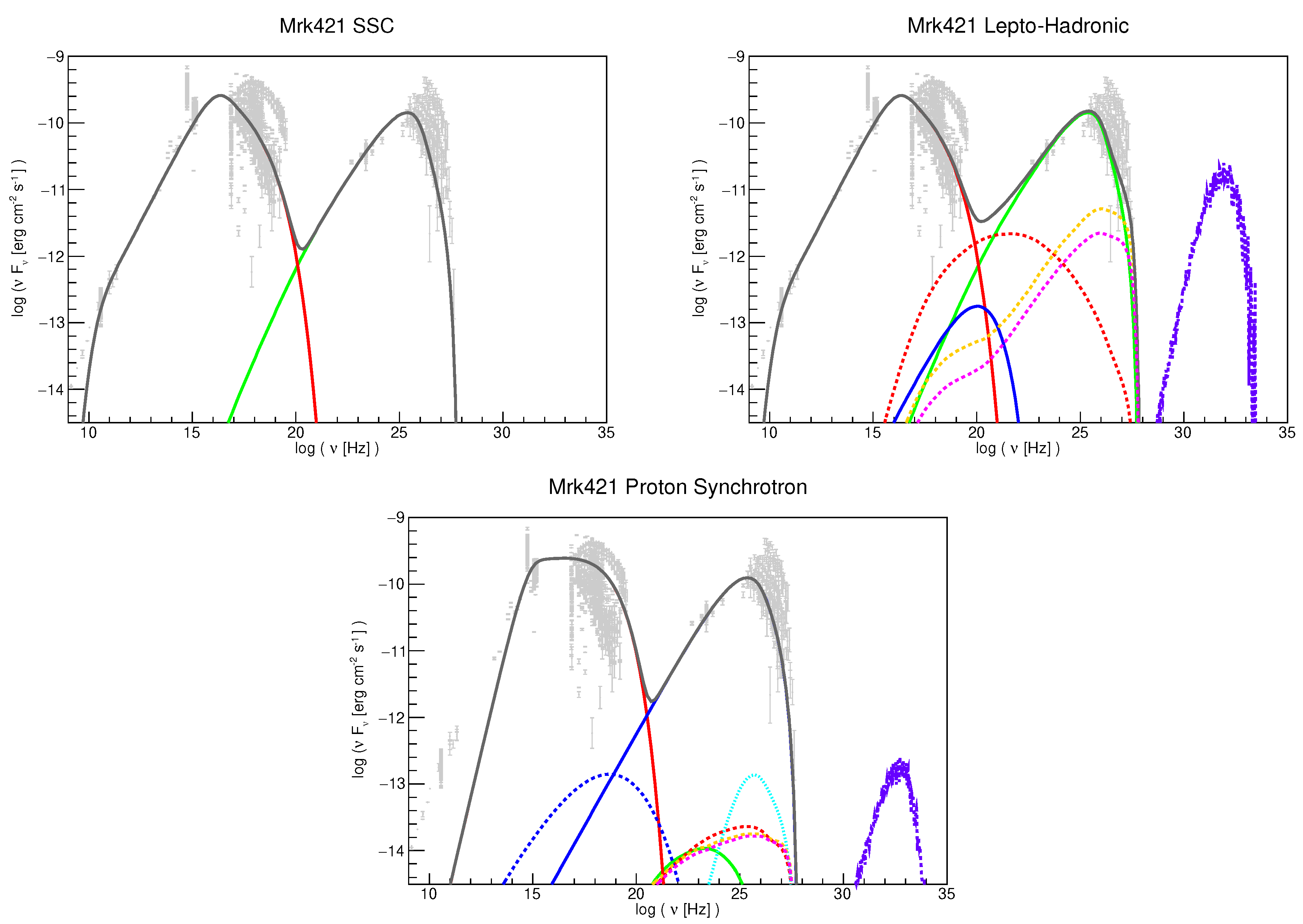
A one-zone SSC model can describe well the SEDs of HBLs (assuming that the radio emission comes from a larger, less dense region in the jet). An example of an SSC modeling of the HBL Markarian 421 is shown in the top-left panel of Figure 2. In the recent years, a number of algorithms have been published to fully constrain the SSC model parameter space, and have been applied successfully to HBLs [63,94,95,96,97]. Typical best-fit solutions are:
where is the electron luminosity in the observer’s frame, and is the electron energy density. The SSC scenario fails to reproduce the SED of other blazar sub-classes: it cannot reproduce the SEDs of LBLs, nor FSRQs; it can reproduce the SEDs of EHBLs at the expenses of a high Doppler factor () and of a high value of [36,98].
2.2.2. Synchrotron-Self-Compton: Time Signatures
Now that we have a model which is able to describe the blazar SEDs (at least for HBLs), we can add the time information to further test it and constrain the parameter values. As for the synchrotron case, we can compute the evolution of the SED with time by solving Equation (7) (including inverse-Compton losses) and calculating both synchrotron and SSC emission as a function of time. One difficulty of SSC time-dependent modeling is that the inverse-Compton cooling term depends on the density of the synchrotron photons, which depends on the integral of the electron distribution itself as a function of time (which is what we want to solve). In presence of significant SSC losses the differential equation becomes thus non-linear and the solution is significantly more complex [99,100]. Blazar light-curves in the -ray band have been successfully fit with the SSC model [79,101]. Similarly to synchrotron radiation, time-lags and hysteresis are also expected in SSC light-curves due to the energy dependency of both the acceleration and cooling terms [102]. But contrarily to what is observed in X-rays, there has not been any significant detection of time-lags or of hysteresis in the -ray band [103,104]. This negative result is likely due to the intrinsic lower sensitivity of gamma-ray telescopes compared to X-ray ones, and not to a failure of the model.
Another important prediction of the SSC scenario is the correlation between the variability of the two SED components, which are expected to vary in concert. If the variability is simply due to an achromatic change in the particle density in the emitting region, the SSC component is expected to vary as the square of the synchrotron component (due to both the change in the particle distribution, and in the synchrotron photons). A correlation plot between X-rays and -rays is thus expected to show a simple quadratic relation. If on the other hand the variability is energy-dependent, the expected correlations are more complex, and depend on the energy bands of the observations, the SED peak frequencies, the energy-dependency of the injection [105]. Correlation studies among different wavebands are indeed a powerful tool to test radiative models when the statistics in an individual band does not allow light-curve fitting [69,106,107,108,109,110].
2.2.3. External Inverse-Compton
Synchrotron photons are not the only low-energy photons that can be up-scattered to -rays. The SMBH environment is very bright, and there is a huge variety of photon fields that can go through inverse-Compton scattering with electrons in the jet. This radiative process is usually called External-inverse-Compton (EIC) and depends strongly on the properties of the external field and on the exact location of the emitting region r (measured from the SMBH). The computation of the EIC component is similar to the SSC one, but requires as first step the transformation of the external photon field distribution into the jet’s frame. For blazar modeling, the relevant photon fields, starting from the AGN core outwards, are:
- the SMBH accretion disk is a reservoir of thermal photons. EIC emission over disk photons is however hindered due to the Doppler deboosting [111]: the plasma in the jet is travelling away from it with Lorentz factor , and thus the disk photon field energy density, in the reference frame of the plasmoid, is strongly suppressed by a factor . EIC scattering over disk photons can thus dominate the overall -ray emission only if the emitting region is located close to the disk itself. In this case the plasma can see part of the disk at angles large enough to reduce the de-boosting.
- the BLR produces bright emission lines (Ly being the dominant one) that can serve as target photon field for EIC emission [112]. In this case the emission is boosted or deboosted in the reference frame of the emitting region as a function of r and . It is important to underline that the BLR is structured, and that different emission lines are produced at different distances from the SMBH. The size of the BLR can be expressed as a function of its luminosity (or other proxies such as the luminosity of the continuum at 5100 Å, or the disk luminosity [6,113]). The EIC emission is thus a superposition of several components coming from the different lines [114], with their relative strength depending on r. A second radiative component coming from the BLR is the photon field from the accretion disk which can be Thomson-scattered by electrons in the BLR and thus seen boosted in the reference frame of the blob. This component depends also on the optical depth of the BLR. A parameter which is not so well known is the aperture angle of the BLR: it can have a spherical geometry () or be flattened over the disk () [115,116]. The assumed BLR geometry has a direct impact on the photon field seen in the blob reference frame, and in the limit of a flat BLR the computation of the associated EIC component becomes similar to the one from the accretion disk.
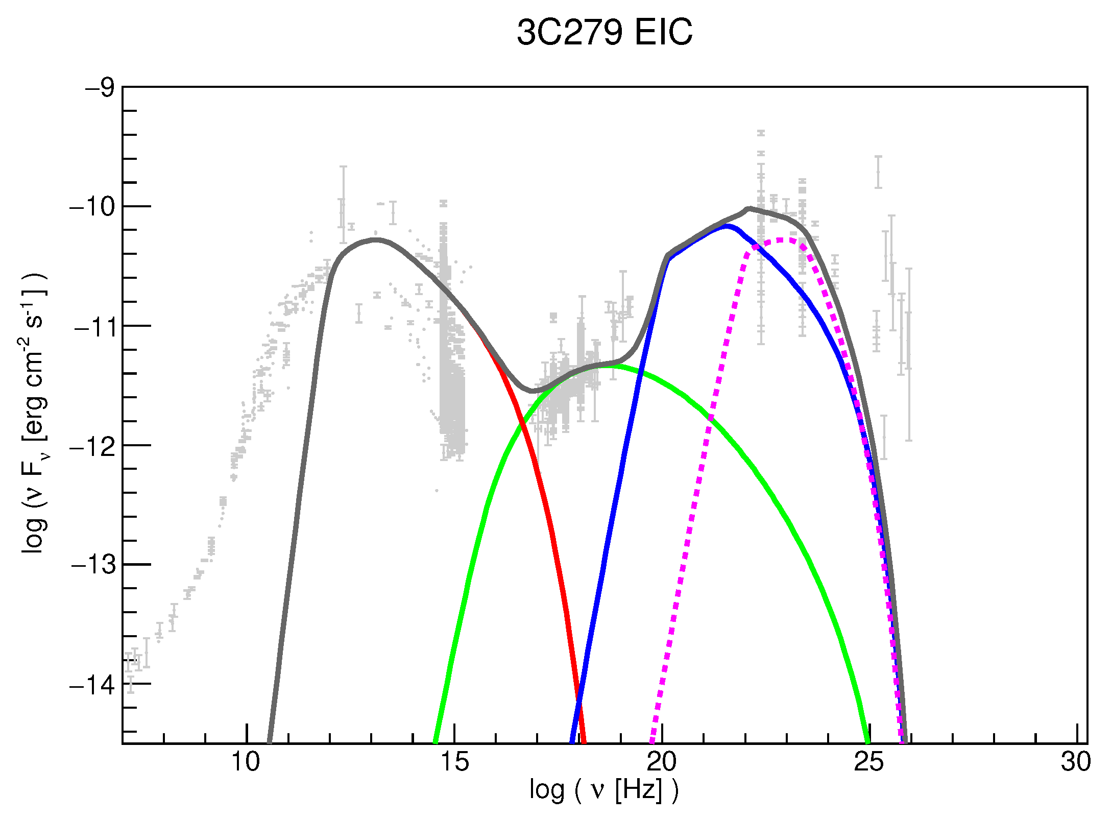
- the emission from the dusty torus is thermal and can be well described with a single-temperature black-body distribution with temperature K. The torus location can also be parametrized as a function of the disk luminosity cm [117]. Similarly to the BLR aperture angle, the aperture angle of the torus is also not well known. It is commonly assumed to be of around . As with the BLR photon field, the blob of plasma sees a constant photon density from the torus for , and then a rapidly decreasing photon field while crossing and leaving the torus behind [118]. An example of an EIC modeling of the FSRQ 3C279 is shown in Figure 3.
- A ubiquitous photon field is the one from the Cosmic Microwave Background (CMB): electrons in the jet can also scatter these photons to higher energies. This EIC emission has the important properties of being the only one dependent on the redshift of the source. EIC over the CMB is not so efficient when the emitting region is located close to the SMBH, because there are always stronger photon fields. But it can become an important radiative process to explain X-ray and -ray emission from SMBH jets at larger scales ([119], but see [120]). lSince the CMB intensity scales as , this emission process can play a more important role for high-redshift quasars [121].
- as we discussed before, structured jets can explain the synchrotron emission from radio up to optical-X-rays. The emission from the other regions of the jet can thus serve as target photon field for EIC scattering. In configurations such as the spine-sheath scenario (a fast inner jet surrounded by a slower layer), the emission from the external jet can be boosted in the -ray emitting region due to the relative motion of the two components [122,123,124].
2.2.4. Energy Budget of the Emitting Region
An important characteristic of all radiative models is its energy budget: how much energy is required to reproduce the observations? and how is energy distributed among the various components? The total jet power (in erg s) can be expressed as an explicit function of the various energy densities as
where the factor of 2 takes into account that there are always two jets.
Equipartition between the various radiative components is always attractive especially in physical systems at equilibrium, because it directly provides a minimum power solution. It is thus interesting to note that SSC solutions for HBLs are not near equipartition, the emitting region being always particle dominated [125,126]. On the other hand, EIC solutions for FSRQs show near-equipartition conditions between particles, magnetic field, and external photons [127].
2.3. Electron-Positron Pair Production
The last leptonic process that is relevant to calculate the radiative output of SMBH jets is pair-production via photon–photon interaction [128]
This process is the inverse of pair annihilation, in which one electron and one positron annihilate into 0.511 MeV photons. Pair-production can occur only if the energy of the two photons is higher than the rest mass of the leptons that are produced, which is . The cross-section of the interaction is [129]
where , and the interaction angle. The cross-section can be reasonably well approximated as
This approximation is known as the -approximation. The pair-production process is more efficient when the energy of the two photons are inversely proportional. The two photons disappear in the interaction, and while for low-energy photon fields the disappearance of a single photon is negligible, for the high-energy photon field a single photon can contribute significantly to the overall energy flux. For -rays, pair-production can result in significant absorption, which can be expressed via the following absorption coefficient (similarly to Equation (5); note that the following equation is correct only if an angle-averaged cross-section is used, otherwise an additional integration over the angle is required):
where is the number density of the low-energy photon field, which can be computed from the intensity
The most relevant - absorption term for -ray blazars is external to the source, and it is represented by the integrated emission from all galaxies (stars and dust) that permeates the Universe, the Extragalactic Background Light (EBL). The EBL acts as an absorber for TeV photons in the Universe, and this absorption effect increases with the distance from Earth and with the energy of the -ray photon [130]. The result is a softening of the spectrum of TeV blazars, and an horizon for TeV astronomy. The TeV horizon is defined as the energy-dependent redshift for which the opacity . Although the EBL significantly hinders TeV observations of distant blazars (the most distant source observed in the TeV band with Cherenkov telescopes is at z = 0.944, although detected only up to 0.175 TeV [131]), this absorption effect can be used to measure the EBL itself, opening up the path to -ray cosmology [132]. The pairs produced in the interaction with the EBL are not lost, and can produce further emission along the line of sight mainly via inverse-Compton scattering over CMB photons, although energy losses from plasma instabilities are also investigated [133]. This emission can be detected both as a new radiative component in the GeV band [134], or as extended gamma-ray pair halos [135], both modulated by the strength of the magnetic field seen by the pairs. None of these features has been detected as per today [136,137,138], and these observations can be used to put constraints on the inter-galactic magnetic field [139,140].
Going back to the inverse-Compton scattering in SMBH jets, all photon fields which are inverse-Compton scattered to -ray energies also act as an absorber to the same -ray photons via pair-production. Let us start by looking at the SSC case. Under the -function approximation for , and by forcing an equality to the causality relation (Equation (22)), it is possible to write , where the pair-production opacity depends only on the Doppler factor (and physical observables) [141], and it is thus possible to provide a lower limit on
where Hz is the frequency of the low-energy photons that act as primary absorber for photons at , and is the index of the flux density at . For typical blazars parameters, Equation (30) results in . The detection of TeV photons from HBLs can thus be used to put a strong limit on , constraining further the parameter space of the SSC model.
2.3.1. On the Location of the -ray Emitting Region in FSRQs
For the EIC case, the opacity to - pair production depends on the location r of the emitting region with respect to the external fields. The opacity is expressed as the integral from r outwards of the absorption coefficient:
The presence of the BLR is very relevant for opacity calculations: if , radiation from the BLR will significantly absorb -ray photons. Assuming that the most relevant emission line is Ly (13.6 eV), this will cause an absorption feature at ≃100 GeV. Detailed calculations including all relevant BLR lines and the thermal continuum from the disk scattered by the BLR [114,142,143,144,145] show that the very detection of -ray photons with energies greater than 100 GeV from FSRQs is enough to put the location of the emitting region beyond the BLR. Observations of FSRQs at GeV confirmed this scenario and proved that, at least for the sources that have been detected at high energies, the emitting region is at or beyond [146,147,148,149,150,151,152].
The dusty torus also leaves an absorption imprint on the -ray spectrum. Given its typical temperature of ≃1000 K, the pair-production absorption on the torus photons is expected to be seen in the TeV band in -ray FSRQs. Due to the simultaneous absorption on the EBL, and to the fact that FSRQs have an SED peak in the 100-MeV range with very few TeV photons, such a cut-off has never been observed as per today [153].
2.3.2. Pair Injection
The electron-positron pairs that have such an important role for -ray absorption in SMBH jet are injected in the emitting region, and can be treated as a secondary injection of leptons. They will behave exactly as the primary ones, and will radiate synchrotron and inverse-Compton photons, reaching their own equilibrium distribution. The big advantage is that while we do not know the details of the primary accelerator and we simply parametrized it, we have the information on the energy distribution of the pairs injected via pair-production [154]:
where and are the photon densities of the two photon fields. The injection term can then be used to compute the steady-state distribution and the associated synchrotron and inverse-Compton emission following Equation (7). For single-zone blazar leptonic models, emission by this secondary leptonic population is usually negligible, hidden by the primary one.
3. Hadronic Radiative Processes
3.1. Proton–Synchrotron Emission
Let us now consider the case of a jet in which there are also protons (and possibly higher-Z nuclei) together with leptons. As with electrons, the proton energy distribution is defined between and as a power-law function:
Going back to our spherical plasmoid in the jet, the first radiative process that needs to be studied is synchrotron radiation by protons.With respect to electrons, the emission from protons is suppressed and needs to be compensated by increasing either the magnetic field value, the particle density, or both. It is interesting to test the possibility that proton–synchrotron radiation is responsible for the high-energy SED component in blazars. Indeed, proton–synchrotron radiation would have the same index as SSC radiation, assuming that the injection index of protons is similar to the one of electrons. Following Equation (19) (replacing the electron mass with the proton mass) it is possible to have a proton–synchrotron peak frequency at around 10-100 GeV, consistent with HBL SEDs, assuming , –100 G, and –50. The proton–synchrotron solution for HBLs lies thus in a completely different part of the parameter space with respect to the SSC solution, with a much stronger (a thousand times higher) magnetic field [155,156,157]. The number of free parameters of the proton–synchrotron scenario is much larger than the SSC one, due to the fact that the proton distribution adds 5 additional free parameters (assuming an additional due to cooling, and the two indexes ), for a total of 14 model parameters. Such a model is clearly degenerate, although the number of free parameters can be considerably reduced by assuming some physically motivated constraints, such as: self-consistency of break Lorentz factors, co-acceleration of electrons and protons (and thus equality of and ), constraint on via equation of acceleration and cooling, constraint on R via causality arguments. But even imposing all these constraints the model remain degenerate, and and we can only constrain allowed regions in the parameter space [98].
3.2. Proton-Photon Interactions
Protons in the jet interact with the low-energy photon fields, both internal (i.e., the electron synchrotron radiation) and external. But contrarily to electrons, for which the dominant interaction is inverse-Compton scattering, the dominant processes for protons are photo-meson production and Bethe–Heitler pair-production. Inverse-Compton scattering for protons does happen, but it can be safely neglected for the modeling of AGN emission.
3.2.1. Photo-Meson Production
The photo-meson (or photo-pion) process is the production of pions in proton-photon interactions:
The photo-meson cross-section is dominated by resonances ( and N baryons), direct pion production and multiple pion production. For astrophysical applications, the relevant information is the production of pions, both neutral and charged. In order to produce pions, the photon energy in the proton frame has to be higher than MeV. In the emitting-region frame, MeV, meaning that protons with Lorentz factor can photo-meson-produce over ultra-violet photons.
Pions then decay primarily ( branching ratio) as
Photo-meson production has thus one key property: neutrinos are produced together with photons, and they can escape the emitting region without suffering from any additional absorption or energy losses. Detection of neutrinos from an AGN is thus a smoking-gun signal for the presence of relativistic protons in the jet. This implies that AGNs can accelerate protons to high energies, and can be responsible for the flux of particles that we call, once they reach Earth, cosmic rays. Joint neutrino and photon observations of AGNs can be used to constrain three key parameters of the model: how many protons are accelerated, what is their energy distribution, and what is their maximum energy.
Together with the neutrinos, photo-meson production injects photons and electron/positron pairs in the emitting region. The spectrum of the injected pions has a maximum energy equal to the proton maximum energy but reduced by the inelasticity . The maximum energy of photons from the decay can be as high as . For protons with , it translates into photons with PeV. These photons do not reach us: they are absorbed via pair-production both in the jet, and in the path to Earth. The absorption occurring in the source produces an electron/positron pair that starts radiating (and cooling). Given the high energy of the first photon, the synchrotron radiation by these secondary leptons is at energies high enough that the synchrotron photons can suffer a second pair-production, and so on. Photons from the decay can thus trigger a synchrotron-supported pair-cascade in the emitting region (or, if the soft photon field energy density is larger than the magnetic one, an inverse-Compton supported pair-cascade). Emission from the cascade can be computed calculating the pair distribution at equilibrium and their synchrotron radiation. When the cascade is saturated, and the resulting synchrotron emission is a power-law with index , or in terms of energy flux : the energy transferred from protons to pions and then to high-energy photons, is then redistributed to low energies.
Electrons and positrons produced in the decay of charged pions go through a process similar to the photons from : they have extremely high-energy, and their synchrotron radiation is also in the PeV band. They thus trigger as well a pair-cascade, which behaves exactly like the one from .
Another important emission process from photo-meson interactions is the synchrotron radiation by . Although not stable leptons, muons in the jet can survive long enough to radiate synchrotron photons before decaying to electrons/positrons. To compute the muon energy distribution at equilibrium, the muon decay term must be added to Equation (7) as follows:
where seconds. The corresponding integral solution for the muon distribution at equilibrium is:
Synchrotron radiation by muons emerges as a third radiative component, at higher energies compared to the synchrotron radiation by the parent protons. In some parts of the parameter space it can represent the dominant radiative emission in the TeV band. Another important consequence is that every time the muon synchrotron radiation is important, it means that muons can cool efficiently before decaying into electrons/positrons, and this energy loss has to be included when calculating their injection in the emitting region.
An interesting property of photo-meson interactions is the creation of neutrons, which can escape the emitting region without interacting with magnetic fields, nor producing Bethe–Heitler pairs (see Section 3.2.2). These neutrons can transfer a significant amount of energy at much larger distances downstream the jet [158,159]. In presence of dense photon fields they can trigger additional photo-meson production, or they can decay into protons (with a life-time of seconds) and radiate again synchrotron photons in the presence of magnetic fields. This “neutral beam” model has drawn attention for its possibility to naturally produce two separate emitting regions in the jet, physically separated but casually connected [160,161].
The main problem we are facing with photo-meson production is that the exact computation of the energy distribution of all secondary particles injected in the emitting region is a complex numerical task. The best approach is to compute them via Monte-Carlo simulations [162]. Several approaches to fit the results of Monte-Carlo simulations and provide a parametrization of the injected secondary particles over a wide parameter space are particularly useful [163,164].
3.2.2. Bethe–Heitler Pair-Production
Bethe–Heitler pair-production is the following process
It is a process which is in competition with the photo-meson production, although it happens at lower energies. The threshold for this interaction is lower than the photo-meson one by a factor . In terms of proton Lorentz factors, protons with can pair-produce over 10 eV photons.
For low-energy protons, the Bethe–Heitler pair production is the main proton-photon interaction, but as soon as the proton energy becomes greater than the energy threshold for photo-meson production, the latter takes over. As expected, pairs injected via this process have a lower energy compared to pairs from the photo-meson [165]. The energy distribution of the injected Bethe–Heitler pairs can be computed analytically [163,166,167], or using a Monte-Carlo approach [168,169]. Their fate is the same as all other leptons in the emitting region: they radiate synchrotron and inverse-Compton photons, and if their energy is high enough (and if the low-energy photon field is dense enough) they can trigger a pair-cascade.
3.3. Hadronic and Lepto-Hadronic Models
Blazar hadronic models are a large family of models which share the presence of a parent population of protons that are accelerated in the SMBH jet. But as discussed above, from the electromagnetic point-of-view the only true hadronic radiative process is proton–synchrotron emission. Solutions in which the high-energy emission is produced by secondary leptons produced in p- interactions are usually referred to as lepto-hadronic models.
Pure hadronic (proton–synchrotron) models can fit blazar SEDs [155,156,157,170], but they face a major problem: the proton density required to fit the data is rather high, and when expressed in terms of it gets close or clearly much higher than the Eddington luminosity of the SMBH [117]. Although should be treated as order-of-magnitude estimate for the available accretion power, if the power in the jet required to fit the data is super-Eddington by several orders of magnitudes it means that either the relation between accretion and jet needs to be revisited, or, more likely, that this particular solution is not viable. This energy-crisis for hadronic models is particularly true for FSRQs [171]. For low-luminosity HBLs and EHBLs it is not the case, and hadronic solutions with can be found [98,172]. Even if the high-energy SED component is dominated by proton–synchrotron radiation, emission by secondary leptons from p- interactions can emerge (namely for compact and dense solutions) in the X-rays and in the TeV band [173,174,175]. In terms of energy budget of the emitting region, proton–synchrotron solutions are out of equipartition, with . An example of a hadronic modeling of the HBL Mrk 421 is shown in the second plot of Figure 2.
In the lepto-hadronic solutions, the proton–synchrotron radiative component is suppressed, and this can be easily achieved by reducing the magnetic field to G. We are back in the part of the parameter space where the SSC emission dominates and indeed the simplest lepto-hadronic model is an SSC solution loaded with relativistic protons that produce secondary leptons via p- interactions over the electron synchrotron photon field (this solution is called one-zone lepto-hadronic model, to highlight the fact that all radiative mechanisms are coming from a single emitting region in the jet, and there external photon fields are negligible). The emission by secondary leptons emerges again in the X-rays (as Bethe–Heitler component) and in the TeV band (as photo-meson component) [172]. This kind of lepto-hadronic solutions are typically more promising in terms of output than pure hadronic solutions. As with hadronic solutions, lepto-hadronic solutions also face energetic issues: especially if the goal of the modeling is to maximize the neutrino output, the required jet power can quickly become very high. A possible way-out to this issue is to use as target photon field not the electron synchrotron radiation, but external photons. By increasing the density of the target photon field, it is possible to achieve the same p- output lowering the required proton power. The discovery of the blazar TXS0506 + 056 as first neutrino blazar candidate [176], indicates that a lepto-hadronic solution over an external field may be the favored scenario [177,178,179,180,181,182]. In terms of energy budget of the emitting region, mixed lepto-hadronic are usually particle dominated, although the result depends on the exact shape of the proton distribution (a soft/hard distribution has a significant impact on , but a marginal effect on the photon and neutrino emission). An example of a mixed lepto-hadronic modeling of the HBL Mrk 421 is shown in the third plot of Figure 2.
Hadronic radiative models are of particular interest any time leptonic ones face difficulties. One of the most interesting cases is the unusual SED of the nearby radio-galaxy Centaurus A, which shows a unique third radiative component emerging at ≃100 GeV [183]. This additional component can be naturally explained in a hadronic or lepto-hadronic scenario [184,185,186].
Among blazar hadronic radiative models, it is worth mentioning another potential contribution produced not in the jet, but rather in the path from the source to the observer. If AGNs accelerate cosmic rays, a hadronic beam can be launched emitting photons and neutrinos while travelling towards Earth [187,188]. So far no evidence for this hadronic contribution has been detected. For a recent study of propagation effects comparing both hadronic cascades and electromagnetic cascades (the ones triggered by the absorption over the EBL) see [189].
Hadronic Models: Time Signatures
From the spectral point of view both leptonic and hadronic radiative models provide similarly good fit to current electromagnetic observations, but they can in principle be distinguished from their temporal behavior. Time-dependent hadronic models require the solution of a system of coupled differential equations of the kind:
for each species X (protons, photons, neutrinos, leptons), where and represents the injection and loss terms, respectively. From a numerical point of view, hadronic time-dependent codes are significantly more complex than leptonic ones, and have been extensively developed only in the recent years [169,190,191,192]. As with leptonic models they can be tested on data in two main ways: fitting light-curve profiles, and studying multi-wavelength correlations.
For proton–synchrotron models, although the two SED components are produced by two distinct particle populations, it is still possible to reproduce the observed correlations assuming that electrons and protons share the same acceleration mechanism [193]. On the other hand, absence of correlations can also be reproduced and indeed, one of the best applications for blazar hadronic models, are the so-called orphan flare, bright -ray flares without multi-wavelength counterparts, which cannot be reproduced in a leptonic one-zone scenario [194,195,196].
Time-dependent models have also the advantage to allow the study of non-linear effects in the development of the hadronic pair-cascades, in which photons from the cascade become targets for pair-production and can result in a unique pulsating signature [197].
3.4. Proton–Proton Interactions
The final hadronic process that needs to be taken into account is pion production in proton–proton interactions. As with the photo-meson production, a highly relativistic proton interacts with a target low-energy proton. For astrophysical applications, the only relevant process is the production of neutral pions and mesons, which then decay into . The result of the interaction is then
where Y and Z are any other particle produced in the interaction. The decay of charged pions is responsible for the associated neutrino emission. As with the photo-meson process, the outcome of proton–proton interactions is better studied via Monte-Carlo simulations, although useful parametrizations have been developed [198,199]. In blazar’s jets, proton–proton interactions represent usually a subdominant contribution. In order to have a significant p-p output a very proton-loaded jet is needed [200]. An alternative scenario is represented by interactions of the jet with obstacles, such as BLR clouds, or stars [201,202,203].
4. Polarization Signatures
An important observable that has the potential to uniquely determine the radiation mechanism, as well as the physical properties of the jet, is polarization. A specific signature of synchrotron radiation is indeed that the emission is linearly polarized. For a power-law electron energy distribution with index n, the maximum polarization fraction is
which is equal to for . Detection of polarized radiation in blazars is thus a key prove that what is observed from radio to optical is synchrotron radiation [204]. The polarization angle can be used to map the orientation of the magnetic field in the jet. Recent multi-wavelength campaigns have shown not only that optical polarization is a characteristic of blazars, but that both the polarization fraction and the polarization angle show drastic variability, often correlated with flares at other wavelengths [205]. For an updated review of optical polarization in AGN jets, see [206] in this special issue. Variability in the optical polarization can also be used to put constraints on the geometry of the emitting regions, and in particular on the relative role of the small plasmoid (the single-zone that emits from optical to gamma-rays) and the larger jet [207,208].
Inverse-Compton scattering is also expected to be polarized, depending on the polarization of the target photon field [209]. X-ray and gamma-ray polarimetry have the potential to significantly constrain blazar radiative models: proton–synchrotron radiation is expected to be significantly much more polarized than SSC radiation or EIC radiation (which is no polarized at all if the external field is also not polarized). Leptonic and hadronic radiative processes can thus be distinguished using this unique observable [210,211].
5. Summary and Perspectives
Relativistic jets from supermassive black holes emit photons over the whole electromagnetic spectrum, from radio to gamma-rays, and since 2017 we have the first evidence that they might be bright in neutrinos as well. The last decades have seen a significant improvement in our knowledge of their gamma-ray emission, and the high-energy peak of their SED is now constrained as well as the low-energy one. These advances on the observational side have significantly constrained our models for the photon emission. The state-of-the-art view is that the most likely emission process in FSRQs is external-inverse-Compton scattering over the bright photon fields around the SMBH environment. If hadronic processes play a role, they should be subdominant in FSRQs, due to the large amount of power they require. For HBLs the main radiation mechanism is SSC, or EIC in a structured jet. In this case, pure hadronic models (proton–synchrotron dominated) cannot be excluded looking at the jet energy budget. Observations of the first blazar neutrino candidate, TXS 0506 + 056, favor a mixed scenario with a leptonic dominated SED with subdominant hadronic components in the form of pair-cascades emerging in the hard-X-rays and the TeV band. X-ray and TeV observations helped identifying a population of blazars with extreme peak frequencies (in the hard-X-rays and the TeV band, respectively), now known as EHBLs: in this case as well it is not possible to disentangle the different radiative mechanisms, and both leptonic and hadronic solutions provide good description of the data. In the upcoming future new observations will provide key constraints on radiative models, and will significantly increase our understanding of the physics of relativistic jets. Neutrino astronomy is just in its early years and additional data from IceCube and its upgrades [212], ANTARES [213], and KM3NET [214] will provide new constraints on hadronic emission processes in AGN jets, whether new neutrino AGNs will be detected, or not. X-ray polarimetry will also impact significantly the field, providing unique constraints on the radiative mechanism responsible for the X-ray emission in AGNs. The Imaging X-ray Polarimetry Explorer (IXPE) satellite [215] is expected to be launched in late 2021. Since they are the most common sources in the gamma-ray sky, answers to the current open problems and new questions on SMBH jets physics will come from the next generation gamma-ray observatories, CTA in the TeV band [216,217], and future proposed MeV observatories, such as AMEGO [218].
Funding
M. Cerruti has received financial support through the Postdoctoral Junior Leader Fellowship Programme from la Caixa Banking Foundation, grant n. LCF/BQ/LI18/11630012. Funding for this work was partially provided by the Spanish MINECO under project MDM-2014-0369 of ICCUB (Unidad de Excelencia ’María de Maeztu’). Silvia Cerruti is acknowledged for the AGN scheme in Figure 1.
Conflicts of Interest
The authors declare no conflict of interest. The funders had no role in the design of the study; in the collection, analyses, or interpretation of data; in the writing of the manuscript, or in the decision to publish the results.
Abbreviations
The following abbreviations are used in this manuscript:
| AGN | Active Galactic Nucleus |
| BLR | Broad Line Region |
| EBL | Extragalactic Background Light |
| EHBL | Extremely High-Frequency Peaked BL Lac objects |
| EIC | External-Inverse-Compton |
| FR | Fanaroff–Riley (I and II) |
| FSRQ | Flat Spectrum Radio Quasar |
| HBL | High-Frequency Peaked BL Lac objects |
| IBL | Intermediate-Frequency Peaked BL Lac objects |
| CDM | -Cold-Dark-Matter |
| LBL | Low-Frequency Peaked BL Lac objects |
| NLR | Narrow Line Region |
| SED | Spectral Energy Distribution |
| SMBH | Supermassive Black Hole |
| SSC | Synchrotron-Self-Compton |
References
- Bañados, E.; Venemans, B.P.; Mazzucchelli, C.; Farina, E.P.; Walter, F.; Wang, F.; Decarli, R.; Stern, D.; Fan, X.; Davies, F.B.; et al. An 800-million-solar-mass black hole in a significantly neutral Universe at a redshift of 7.5. Nature 2018, 553, 473–476. [Google Scholar] [CrossRef] [PubMed] [Green Version]
- Aghanim, N.; Akrami, Y.; Ashdown, M.; Aumont, J.; Baccigalupi, C.; Ballardini, M.; Banday, A.J.; Barreiro, R.B.; Bartolo, N.; Basak, S.; et al. Planck 2018 results. VI. Cosmological parameters. arXiv 2018, arXiv:1807.06209. [Google Scholar]
- Akiyama, K.; Alberdi, A.; Alef, W.; Asada, K.; Azulay, R.; Baczko, A.K.; Ball, D.; Baloković, M.; Barrett, J.; Bintley, D.; et al. First M87 Event Horizon Telescope Results. I. The Shadow of the Supermassive Black Hole. Astrophys. J. Lett. 2019, 875, L1. [Google Scholar] [CrossRef]
- Abramowicz, M.A.; Fragile, P.C. Foundations of Black Hole Accretion Disk Theory. Living Rev. Relativ. 2013, 16, 1. [Google Scholar] [CrossRef] [Green Version]
- Jaffe, W.; Ford, H.C.; Ferrarese, L.; van den Bosch, F.; O’Connell, R.W. A large nuclear accretion disk in the active galaxy NGC4261. Nature 1993, 364, 213–215. [Google Scholar] [CrossRef]
- Greene, J.E.; Ho, L.C. Estimating Black Hole Masses in Active Galaxies Using the Hα Emission Line. Astrophys. J. 2005, 630, 122–129. [Google Scholar] [CrossRef]
- Bentz, M.C.; Walsh, J.L.; Barth, A.J.; Baliber, N.; Bennert, V.N.; Canalizo, G.; Filippenko, A.V.; Ganeshalingam, M.; Gates, E.L.; Greene, J.E.; et al. The Lick AGN Monitoring Project: Broad-line Region Radii and Black Hole Masses from Reverberation Mapping of Hβ. Astrophys. J. 2009, 705, 199–217. [Google Scholar] [CrossRef]
- Bennert, N.; Falcke, H.; Schulz, H.; Wilson, A.S.; Wills, B.J. Size and Structure of the Narrow-Line Region of Quasars. Astrophys. J. Lett. 2002, 574, L105–L109. [Google Scholar] [CrossRef] [Green Version]
- Netzer, H. Revisiting the Unified Model of Active Galactic Nuclei. Annu. Rev. Astron. Astrophys. 2015, 53, 365–408. [Google Scholar] [CrossRef] [Green Version]
- Schmidt, M. 3C 273: A Star-Like Object with Large Red-Shift. Nature 1963, 197, 1040. [Google Scholar] [CrossRef]
- Bahcall, J.N.; Kirhakos, S.; Saxe, D.H.; Schneider, D.P. Hubble Space Telescope Images of a Sample of 20 Nearby Luminous Quasars. Astrophys. J. 1997, 479, 642–658. [Google Scholar] [CrossRef] [Green Version]
- Wilson, A.S.; Colbert, E.J.M. The Difference between Radio-loud and Radio-quiet Active Galaxies. Astrophys. J. 1995, 438, 62. [Google Scholar] [CrossRef] [Green Version]
- Kellermann, K.I.; Vermeulen, R.C.; Zensus, J.A.; Cohen, M.H. Sub-Milliarcsecond Imaging of Quasars and Active Galactic Nuclei. Astron. J. 1998, 115, 1295–1318. [Google Scholar] [CrossRef]
- Butcher, H.R.; van Breugel, W.; Miley, G.K. Optical observations of radio jets. Astrophys. J. 1980, 235, 749–754. [Google Scholar] [CrossRef] [Green Version]
- Marshall, H.L.; Schwartz, D.A.; Lovell, J.E.J.; Murphy, D.W.; Worrall, D.M.; Birkinshaw, M.; Gelbord, J.M.; Perlman, E.S.; Jauncey, D.L. A Chandra Survey of Quasar Jets: First Results. Astrophys. J. Suppl. 2005, 156, 13–33. [Google Scholar] [CrossRef] [Green Version]
- Abdo, A.A.; Ackermann, M.; Ajello, M.; Atwood, W.B.; Baldini, L.; Ballet, J.; Barbiellini, G.; Bastieri, D.; Baughman, B.M.; Bechtol, K.; et al. Fermi Gamma-Ray Imaging of a Radio Galaxy. Science 2010, 328, 725. [Google Scholar] [CrossRef] [Green Version]
- De Naurois, M. Resolving the kpc jet of Centaurus A in TeV gamma-rays. In Proceedings of the 36th International Cosmic Ray Conference (ICRC2019), Madison, WI, USA, 1 August 2019; Volume 36, p. 657. [Google Scholar]
- Blandford, R.D.; Rees, M.J. Extended and compact extragalactic radio sources: Interpretation and theory. Phys. Scr. 1978, 17, 265–274. [Google Scholar] [CrossRef]
- Blandford, R.D.; Königl, A. Relativistic jets as compact radio sources. Astrophys. J. 1979, 232, 34–48. [Google Scholar] [CrossRef]
- Urry, C.M.; Padovani, P. Unified Schemes for Radio-Loud Active Galactic Nuclei. Publ. Astron. Soc. Pac. 1995, 107, 803. [Google Scholar] [CrossRef] [Green Version]
- Angel, J.R.P.; Stockman, H.S. Optical and infrared polarization of active extragalactic objects. Annu. Rev. Astron. Astrophys. 1980, 18, 321–361. [Google Scholar] [CrossRef]
- The Fermi-LAT Collaboration. Fermi Large Area Telescope Fourth Source Catalog. arXiv 2019, arXiv:1902.10045. [Google Scholar]
- Shaw, M.S.; Romani, R.W.; Cotter, G.; Healey, S.E.; Michelson, P.F.; Readhead, A.C.S.; Richards, J.L.; Max-Moerbeck, W.; King, O.G.; Potter, W.J. Spectroscopy of the Largest Ever γ-Ray-selected BL Lac Sample. Astrophys. J. 2013, 764, 135. [Google Scholar] [CrossRef] [Green Version]
- Shaw, M.S.; Romani, R.W.; Cotter, G.; Healey, S.E.; Michelson, P.F.; Readhead, A.C.S.; Richards, J.L.; Max-Moerbeck, W.; King, O.G.; Potter, W.J. Spectroscopy of Broad-line Blazars from 1LAC. Astrophys. J. 2012, 748, 49. [Google Scholar] [CrossRef]
- Fanaroff, B.L.; Riley, J.M. The morphology of extragalactic radio sources of high and low luminosity. Mon. Not. R. Astron. Soc. 1974, 167, 31P–36P. [Google Scholar] [CrossRef] [Green Version]
- Lister, M.L.; Aller, M.F.; Aller, H.D.; Homan, D.C.; Kellermann, K.I.; Kovalev, Y.Y.; Pushkarev, A.B.; Richards, J.L.; Ros, E.; Savolainen, T. MOJAVE. X. Parsec-scale Jet Orientation Variations and Superluminal Motion in Active Galactic Nuclei. Astron. J. 2013, 146, 120. [Google Scholar] [CrossRef] [Green Version]
- Hartman, R.C.; Bertsch, D.L.; Fichtel, C.E.; Hunter, S.D.; Kanbach, G.; Kniffen, D.A.; Kwok, P.W.; Lin, Y.C.; Mattox, J.R.; Mayer-Hasselwander, H.A.; et al. Detection of High-Energy Gamma Radiation from Quasar 3C 279 by the EGRET Telescope on the Compton Gamma Ray Observatory. Astrophys. J. Lett. 1992, 385, L1. [Google Scholar] [CrossRef]
- Punch, M.; Akerlof, C.W.; Cawley, M.F.; Chantell, M.; Fegan, D.J.; Fennell, S.; Gaidos, J.A.; Hagan, J.; Hillas, A.M.; Jiang, Y.; et al. Detection of TeV photons from the active galaxy Markarian 421. Nature 1992, 358, 477–478. [Google Scholar] [CrossRef] [Green Version]
- Padovani, P.; Giommi, P. The Connection between X-ray- and Radio-selected BL Lacertae Objects. Astrophys. J. 1995, 444, 567. [Google Scholar] [CrossRef] [Green Version]
- Abdo, A.A.; Ackermann, M.; Agudo, I.; Ajello, M.; Aller, H.D.; Aller, M.F.; Angelakis, E.; Arkharov, A.A.; Axelsson, M.; Bach, U.; et al. The Spectral Energy Distribution of Fermi Bright Blazars. Astrophys. J. 2010, 716, 30–70. [Google Scholar] [CrossRef] [Green Version]
- Laurent-Muehleisen, S.A.; Kollgaard, R.I.; Feigelson, E.D.; Brinkmann, W.; Siebert, J. The RGB Sample of Intermediate BL Lacertae Objects. Astrophys. J. 1999, 525, 127–143. [Google Scholar] [CrossRef] [Green Version]
- Costamante, L.; Ghisellini, G.; Giommi, P.; Tagliaferri, G.; Celotti, A.; Chiaberge, M.; Fossati, G.; Maraschi, L.; Tavecchio, F.; Treves, A.; et al. Extreme synchrotron BL Lac objects. Stretching the blazar sequence. Astron. Astrophys. 2001, 371, 512–526. [Google Scholar] [CrossRef] [Green Version]
- Bonnoli, G.; Tavecchio, F.; Ghisellini, G.; Sbarrato, T. An emerging population of BL Lacs with extreme properties: Towards a class of EBL and cosmic magnetic field probes? Mon. Not. R. Astron. Soc. 2015, 451, 611–621. [Google Scholar] [CrossRef] [Green Version]
- Aharonian, F.; Akhperjanian, A.G.; Barres de Almeida, U.; Bazer-Bachi, A.R.; Behera, B.; Beilicke, M.; Benbow, W.; Bernlöhr, K.; Boisson, C.; Bolz, O.; et al. New constraints on the mid-IR EBL from the HESS discovery of VHE γ-rays from 1ES 0229+200. Astron. Astrophys. 2007, 475, L9–L13. [Google Scholar] [CrossRef] [Green Version]
- Foffano, L.; Prandini, E.; Franceschini, A.; Paiano, S. A new hard X-ray-selected sample of extreme high-energy peaked BL Lac objects and their TeV gamma-ray properties. Mon. Not. R. Astron. Soc. 2019, 486, 1741–1762. [Google Scholar] [CrossRef]
- Biteau, J.; Prandini, E.; Costamante, L.; Lemoine, M.; Padovani, P.; Pueschel, E.; Resconi, E.; Tavecchio, F.; Taylor, A.; Zech, A. Progress in unveiling extreme particle acceleration in persistent astrophysical jets. Nat. Astron. 2020, 4, 124–131. [Google Scholar] [CrossRef] [Green Version]
- Costamante, L. TeV-peaked candidate BL Lac objects. Mon. Not. R. Astron. Soc. 2020, 491, 2771–2778. [Google Scholar] [CrossRef] [Green Version]
- Fossati, G.; Maraschi, L.; Celotti, A.; Comastri, A.; Ghisellini, G. A unifying view of the spectral energy distributions of blazars. Mon. Not. R. Astron. Soc. 1998, 299, 433–448. [Google Scholar] [CrossRef]
- Meyer, E.T.; Fossati, G.; Georganopoulos, M.; Lister, M.L. From the Blazar Sequence to the Blazar Envelope: Revisiting the Relativistic Jet Dichotomy in Radio-loud Active Galactic Nuclei. Astrophys. J. 2011, 740, 98. [Google Scholar] [CrossRef] [Green Version]
- Ghisellini, G.; Righi, C.; Costamante, L.; Tavecchio, F. The Fermi blazar sequence. Mon. Not. R. Astron. Soc. 2017, 469, 255–266. [Google Scholar] [CrossRef]
- Padovani, P.; Perlman, E.S.; Landt, H.; Giommi, P.; Perri, M. What Types of Jets Does Nature Make? A New Population of Radio Quasars. Astrophys. J. 2003, 588, 128–142. [Google Scholar] [CrossRef] [Green Version]
- Nieppola, E.; Valtaoja, E.; Tornikoski, M.; Hovatta, T.; Kotiranta, M. Blazar sequence—An artefact of Doppler boosting. Astron. Astrophys. 2008, 488, 867–872. [Google Scholar] [CrossRef]
- Padovani, P.; Giommi, P.; Rau, A. The discovery of high-power high synchrotron peak blazars. Mon. Not. R. Astron. Soc. 2012, 422, L48–L52. [Google Scholar] [CrossRef] [Green Version]
- Giommi, P.; Padovani, P.; Polenta, G.; Turriziani, S.; D’Elia, V.; Piranomonte, S. A simplified view of blazars: Clearing the fog around long-standing selection effects. Mon. Not. R. Astron. Soc. 2012, 420, 2899–2911. [Google Scholar] [CrossRef]
- Böttcher, M.; Dermer, C.D. An Evolutionary Scenario for Blazar Unification. Astrophys. J. 2002, 564, 86–91. [Google Scholar] [CrossRef] [Green Version]
- Ghisellini, G.; Tavecchio, F. The blazar sequence: A new perspective. Mon. Not. R. Astron. Soc. 2008, 387, 1669–1680. [Google Scholar] [CrossRef]
- Finke, J.D. Compton Dominance and the Blazar Sequence. Astrophys. J. 2013, 763, 134. [Google Scholar] [CrossRef] [Green Version]
- Blandford, R.; Meier, D.; Readhead, A. Relativistic Jets from Active Galactic Nuclei. Annu. Rev. Astron. Astrophys. 2019, 57, 467–509. [Google Scholar] [CrossRef] [Green Version]
- Hovatta, T.; Lindfors, E. Relativistic Jets of Blazars. arXiv 2020, arXiv:2003.06322. [Google Scholar]
- Romero, G.E.; Boettcher, M.; Markoff, S.; Tavecchio, F. Relativistic Jets in Active Galactic Nuclei and Microquasars. Space Sci. Rev. 2017, 207, 5–61. [Google Scholar] [CrossRef]
- Kirk, J.G.; Guthmann, A.W.; Gallant, Y.A.; Achterberg, A. Particle Acceleration at Ultrarelativistic Shocks: An Eigenfunction Method. Astrophys. J. 2000, 542, 235–242. [Google Scholar] [CrossRef] [Green Version]
- Sironi, L.; Petropoulou, M.; Giannios, D. Relativistic jets shine through shocks or magnetic reconnection? Mon. Not. R. Astron. Soc. 2015, 450, 183–191. [Google Scholar] [CrossRef]
- Blumenthal, G.R.; Gould, R.J. Bremsstrahlung, Synchrotron Radiation, and Compton Scattering of High-Energy Electrons Traversing Dilute Gases. Rev. Mod. Phys. 1970, 42, 237–271. [Google Scholar] [CrossRef]
- Rybicki, G.B.; Lightman, A.P. Radiative Processes in Astrophysics; Wiley: Hoboken, NJ, USA, 1979. [Google Scholar]
- Longair, M.S. High Energy Astrophysics. Volume 2. Stars, the Galaxy and the Interstellar Medium; Cambridge University Press: Cambridge, UK, 1994; Volume 2. [Google Scholar]
- Dermer, C.D.; Menon, G. High Energy Radiation from Black Holes: Gamma Rays, Cosmic Rays, and Neutrinos; Princeton University Press: Princeton, NJ, USA, 2009. [Google Scholar]
- Bloom, S.D.; Marscher, A.P. An Analysis of the Synchrotron Self-Compton Model for the Multi—Wave Band Spectra of Blazars. Astrophys. J. 1996, 461, 657. [Google Scholar] [CrossRef]
- Inoue, S.; Takahara, F. Electron Acceleration and Gamma-Ray Emission from Blazars. Astrophys. J. 1996, 463, 555. [Google Scholar] [CrossRef]
- Kardashev, N.S. Nonstationarity of Spectra of Young Sources of Nonthermal Radio Emission. Sov. Astron. 1962, 6, 317. [Google Scholar]
- Saugé, L.; Henri, G. TeV Blazar Gamma-Ray Emission Produced by a Cooling Pileup Particle Energy Distribution Function. Astrophys. J. 2004, 616, 136–146. [Google Scholar] [CrossRef]
- Sari, R.; Esin, A.A. On the Synchrotron Self-Compton Emission from Relativistic Shocks and Its Implications for Gamma-Ray Burst Afterglows. Astrophys. J. 2001, 548, 787–799. [Google Scholar] [CrossRef] [Green Version]
- Tavecchio, F.; Ghisellini, G.; Ghirlanda, G.; Foschini, L.; Maraschi, L. TeV BL Lac objects at the dawn of the Fermi era. Mon. Not. R. Astron. Soc. 2010, 401, 1570–1586. [Google Scholar] [CrossRef] [Green Version]
- Zhang, J.; Liang, E.W.; Zhang, S.N.; Bai, J.M. Radiation Mechanisms and Physical Properties of GeV-TeV BL Lac Objects. Astrophys. J. 2012, 752, 157. [Google Scholar] [CrossRef]
- Aharonian, F.; Akhperjanian, A.G.; Barres de Almeida, U.; Bazer-Bachi, A.R.; Behera, B.; Beilicke, M.; Benbow, W.; Bernlöhr, K.; Boisson, C.; Borrel, V.; et al. Discovery of VHE γ-rays from the high-frequency-peaked BL Lacertae object RGB J0152+017. Astron. Astrophys. 2008, 481, L103–L107. [Google Scholar] [CrossRef]
- Aleksić, J.; Ansoldi, S.; Antonelli, L.A.; Antoranz, P.; Babic, A.; Bangale, P.; Barres de Almeida, U.; Barrio, J.A.; Becerra González, J.; Bednarek, W.; et al. Discovery of very high energy γ-ray emission from the blazar 1ES 0033+595 by the MAGIC telescopes. Mon. Not. R. Astron. Soc. 2015, 446, 217–225. [Google Scholar] [CrossRef] [Green Version]
- Archambault, S.; Archer, A.; Beilicke, M.; Benbow, W.; Bird, R.; Biteau, J.; Bouvier, A.; Bugaev, V.; Cardenzana, J.V.; Cerruti, M.; et al. VERITAS Detection of γ-Ray Flaring Activity From the BL Lac Object 1ES 1727+502 During Bright Moonlight Observations. Astrophys. J. 2015, 808, 110. [Google Scholar] [CrossRef]
- Abramowski, A.; Acero, F.; Aharonian, F.; Akhperjanian, A.G.; Anton, G.; Barnacka, A.; Barres de Almeida, U.; Bazer-Bachi, A.R.; Becherini, Y.; Becker, J.; et al. Simultaneous multi-wavelength campaign on PKS 2005-489 in a high state. Astron. Astrophys. 2011, 533, A110. [Google Scholar] [CrossRef]
- Aliu, E.; Archambault, S.; Arlen, T.; Aune, T.; Beilicke, M.; Benbow, W.; Bird, R.; Bouvier, A.; Buckley, J.H.; Bugaev, V.; et al. Long Term Observations of B2 1215+30 with VERITAS. Astrophys. J. 2013, 779, 92. [Google Scholar] [CrossRef] [Green Version]
- Baloković, M.; Paneque, D.; Madejski, G.; Furniss, A.; Chiang, J.; Ajello, M.; Alexander, D.M.; Barret, D.; Blandford, R.D.; Boggs, S.E.; et al. Multiwavelength Study of Quiescent States of Mrk 421 with Unprecedented Hard X-ray Coverage Provided by NuSTAR in 2013. Astrophys. J. 2016, 819, 156. [Google Scholar] [CrossRef] [Green Version]
- Marscher, A.P. Turbulent, Extreme Multi-zone Model for Simulating Flux and Polarization Variability in Blazars. Astrophys. J. 2014, 780, 87. [Google Scholar] [CrossRef]
- Chiang, J.; Böttcher, M. Synchrotron and Synchrotron Self-Compton Spectral Signatures and Blazar Emission Models. Astrophys. J. 2002, 564, 92–96. [Google Scholar] [CrossRef]
- Graff, P.B.; Georganopoulos, M.; Perlman, E.S.; Kazanas, D. A Multizone Model for Simulating the High-Energy Variability of TeV Blazars. Astrophys. J. 2008, 689, 68–78. [Google Scholar] [CrossRef] [Green Version]
- Massaro, E.; Perri, M.; Giommi, P.; Nesci, R. Log-parabolic spectra and particle acceleration in the BL Lac object Mkn 421: Spectral analysis of the complete BeppoSAX wide band X-ray data set. Astron. Astrophys. 2004, 413, 489–503. [Google Scholar] [CrossRef]
- Tramacere, A.; Giommi, P.; Perri, M.; Verrecchia, F.; Tosti, G. Swift observations of the very intense flaring activity of Mrk 421 during 2006. I. Phenomenological picture of electron acceleration and predictions for MeV/GeV emission. Astron. Astrophys. 2009, 501, 879–898. [Google Scholar] [CrossRef] [Green Version]
- Sol, H.; Pelletier, G.; Asseo, E. Two-flow model for extragalactic radio jets. Mon. Not. R. Astron. Soc. 1989, 237, 411–429. [Google Scholar] [CrossRef] [Green Version]
- Ghisellini, G.; Maraschi, L.; Treves, A. Inhomogeneous synchrotron-self-compton models and the problem of relativistic beaming of BL Lac objects. Astron. Astrophys. 1985, 146, 204–212. [Google Scholar]
- Potter, W.J.; Cotter, G. Synchrotron and inverse-Compton emission from blazar jets—I. A uniform conical jet model. Mon. Not. R. Astron. Soc. 2012, 423, 756–765. [Google Scholar] [CrossRef] [Green Version]
- Archer, A.; Benbow, W.; Bird, R.; Brose, R.; Buchovecky, M.; Bugaev, V.; Cui, W.; Daniel, M.K.; Falcone, A.; Feng, Q.; et al. HESS J1943+213: An Extreme Blazar Shining through the Galactic Plane. Astrophys. J. 2018, 862, 41. [Google Scholar] [CrossRef] [Green Version]
- Abramowski, A.; Acero, F.; Aharonian, F.; Akhperjanian, A.G.; Anton, G.; Balzer, A.; Barnacka, A.; Barres de Almeida, U.; Becherini, Y.; Becker, J.; et al. A multiwavelength view of the flaring state of PKS 2155-304 in 2006. Astron. Astrophys. 2012, 539, A149. [Google Scholar] [CrossRef]
- Ahnen, M.L.; Ansoldi, S.; Antonelli, L.A.; Antoranz, P.; Babic, A.; Banerjee, B.; Bangale, P.; Barres de Almeida, U.; Barrio, J.A.; Becerra González, J.; et al. Investigating the peculiar emission from the new VHE gamma-ray source H1722+119. Mon. Not. R. Astron. Soc. 2016, 459, 3271–3281. [Google Scholar] [CrossRef] [Green Version]
- Mastichiadis, A.; Kirk, J.G. Variability in the synchrotron self-Compton model of blazar emission. Astron. Astrophys. 1997, 320, 19–25. [Google Scholar]
- Kirk, J.G.; Rieger, F.M.; Mastichiadis, A. Particle acceleration and synchrotron emission in blazar jets. Astron. Astrophys. 1998, 333, 452–458. [Google Scholar]
- Böttcher, M.; Chiang, J. X-ray Spectral Variability Signatures of Flares in BL Lacertae Objects. Astrophys. J. 2002, 581, 127–142. [Google Scholar] [CrossRef]
- Takahashi, T.; Tashiro, M.; Madejski, G.; Kubo, H.; Kamae, T.; Kataoka, J.; Kii, T.; Makino, F.; Makishima, K.; Yamasaki, N. ASCA Observation of an X-ray/TeV Flare from the BL Lacertae Object Markarian 421. Astrophys. J. Lett. 1996, 470, L89. [Google Scholar] [CrossRef]
- Kataoka, J.; Takahashi, T.; Makino, F.; Inoue, S.; Madejski, G.M.; Tashiro, M.; Urry, C.M.; Kubo, H. Variability Pattern and the Spectral Evolution of the BL Lacertae Object PKS 2155-304. Astrophys. J. 2000, 528, 243–253. [Google Scholar] [CrossRef] [Green Version]
- Zhang, Y.H.; Treves, A.; Celotti, A.; Chiappetti, L.; Fossati, G.; Ghisellini, G.; Maraschi, L.; Pian, E.; Tagliaferri, G.; Tavecchio, F. Four Years of Monitoring Blazar PKS 2155-304 with BeppoSAX: Probing the Dynamics of the Jet. Astrophys. J. 2002, 572, 762–785. [Google Scholar] [CrossRef] [Green Version]
- Sokolov, A.; Marscher, A.P.; McHardy, I.M. Synchrotron Self-Compton Model for Rapid Nonthermal Flares in Blazars with Frequency-dependent Time Lags. Astrophys. J. 2004, 613, 725–746. [Google Scholar] [CrossRef] [Green Version]
- Chiaberge, M.; Ghisellini, G. Rapid variability in the synchrotron self-Compton model for blazars. Mon. Not. R. Astron. Soc. 1999, 306, 551–560. [Google Scholar] [CrossRef] [Green Version]
- Klein, O.; Nishina, T. Über die Streuung von Strahlung durch freie Elektronen nach der neuen relativistischen Quantendynamik von Dirac. Z. Phys. 1929, 52, 853–868. [Google Scholar] [CrossRef]
- Jones, F.C. Calculated Spectrum of Inverse-Compton-Scattered Photons. Phys. Rev. 1968, 167, 1159–1169. [Google Scholar] [CrossRef] [Green Version]
- Moderski, R.; Sikora, M.; Coppi, P.S.; Aharonian, F. Klein-Nishina effects in the spectra of non-thermal sources immersed in external radiation fields. Mon. Not. R. Astron. Soc. 2005, 363, 954–966. [Google Scholar] [CrossRef] [Green Version]
- Gould, R.J. Compton and synchrotron processes in spherically-symmetric non-thermal sources. Astron. Astrophys. 1979, 76, 306–311. [Google Scholar]
- Tavecchio, F.; Maraschi, L.; Ghisellini, G. Constraints on the Physical Parameters of TeV Blazars. Astrophys. J. 1998, 509, 608–619. [Google Scholar] [CrossRef] [Green Version]
- Finke, J.D.; Dermer, C.D.; Böttcher, M. Synchrotron Self-Compton Analysis of TeV X-ray-Selected BL Lacertae Objects. Astrophys. J. 2008, 686, 181–194. [Google Scholar] [CrossRef]
- Mankuzhiyil, N.; Ansoldi, S.; Persic, M.; Tavecchio, F. The Environment and Distribution of Emitting Electrons as a Function of Source Activity in Markarian 421. Astrophys. J. 2011, 733, 14. [Google Scholar] [CrossRef] [Green Version]
- Cerruti, M.; Boisson, C.; Zech, A. Constraining the parameter space of the one-zone synchrotron-self-Compton model for GeV-TeV detected BL Lacertae objects. Astron. Astrophys. 2013, 558, A47. [Google Scholar] [CrossRef] [Green Version]
- Ahnen, M.L.; Ansoldi, S.; Antonelli, L.A.; Antoranz, P.; Babic, A.; Banerjee, B.; Bangale, P.; Barres de Almeida, U.; Barrio, J.A.; Becerra González, J.; et al. Multiband variability studies and novel broadband SED modeling of Mrk 501 in 2009. Astron. Astrophys. 2017, 603, A31. [Google Scholar] [CrossRef]
- Cerruti, M.; Zech, A.; Boisson, C.; Inoue, S. A hadronic origin for ultra-high-frequency-peaked BL Lac objects. Mon. Not. R. Astron. Soc. 2015, 448, 910–927. [Google Scholar] [CrossRef]
- Zacharias, M.; Schlickeiser, R. Blazar synchrotron emission of instantaneously power-law injected electrons under linear synchrotron, non-linear SSC, and combined synchrotron-SSC cooling. Astron. Astrophys. 2010, 524, A31. [Google Scholar] [CrossRef] [Green Version]
- Zacharias, M. Inverse Compton light curves of blazars under non-linear, time-dependent synchrotron-self Compton cooling. Mon. Not. R. Astron. Soc. 2014, 443, 3001–3021. [Google Scholar] [CrossRef] [Green Version]
- Chen, X.; Fossati, G.; Liang, E.P.; Böttcher, M. Time-dependent simulations of multiwavelength variability of the blazar Mrk 421 with a Monte Carlo multizone code. Mon. Not. R. Astron. Soc. 2011, 416, 2368–2387. [Google Scholar] [CrossRef] [Green Version]
- Perennes, C.; Sol, H.; Bolmont, J. Modeling spectral lags in active galactic nucleus flares in the context of Lorentz invariance violation searches. Astron. Astrophys. 2020, 633, A143. [Google Scholar] [CrossRef]
- Albert, J.; Aliu, E.; Anderhub, H.; Antoranz, P.; Armada, A.; Baixeras, C.; Barrio, J.A.; Bartko, H.; Bastieri, D.; Becker, J.K.; et al. Variable Very High Energy γ-Ray Emission from Markarian 501. Astrophys. J. 2007, 669, 862–883. [Google Scholar] [CrossRef] [Green Version]
- Abeysekara, A.U.; Archambault, S.; Archer, A.; Benbow, W.; Bird, R.; Buchovecky, M.; Buckley, J.H.; Bugaev, V.; Cardenzana, J.V.; Cerruti, M.; et al. A Search for Spectral Hysteresis and Energy-dependent Time Lags from X-ray and TeV Gamma-Ray Observations of Mrk 421. Astrophys. J. 2017, 834, 2. [Google Scholar] [CrossRef] [Green Version]
- Katarzyński, K.; Ghisellini, G.; Tavecchio, F.; Maraschi, L.; Fossati, G.; Mastichiadis, A. Correlation between the TeV and X-ray emission in high-energy peaked BL Lac objects. Astron. Astrophys. 2005, 433, 479–496. [Google Scholar] [CrossRef]
- Fossati, G.; Buckley, J.H.; Bond, I.H.; Bradbury, S.M.; Carter-Lewis, D.A.; Chow, Y.C.K.; Cui, W.; Falcone, A.D.; Finley, J.P.; Gaidos, J.A.; et al. Multiwavelength Observations of Markarian 421 in 2001 March: An Unprecedented View on the X-ray/TeV Correlated Variability. Astrophys. J. 2008, 677, 906–925. [Google Scholar] [CrossRef] [Green Version]
- Acciari, V.A.; Aliu, E.; Arlen, T.; Aune, T.; Beilicke, M.; Benbow, W.; Boltuch, D.; Bradbury, S.M.; Buckley, J.H.; Bugaev, V.; et al. TeV and Multi-wavelength Observations of Mrk 421 in 2006–2008. Astrophys. J. 2011, 738, 25. [Google Scholar] [CrossRef] [Green Version]
- Aleksić, J.; Ansoldi, S.; Antonelli, L.A.; Antoranz, P.; Babic, A.; Bangale, P.; Barres de Almeida, U.; Barrio, J.A.; Becerra González, J.; Bednarek, W.; et al. Unprecedented study of the broadband emission of Mrk 421 during flaring activity in March 2010. Astron. Astrophys. 2015, 578, A22. [Google Scholar] [CrossRef]
- Furniss, A.; Noda, K.; Boggs, S.; Chiang, J.; Christensen, F.; Craig, W.; Giommi, P.; Hailey, C.; Harisson, F.; Madejski, G.; et al. First NuSTAR Observations of Mrk 501 within a Radio to TeV Multi-Instrument Campaign. Astrophys. J. 2015, 812, 65. [Google Scholar] [CrossRef]
- González, M.M.; Patricelli, B.; Fraija, N.; García-González, J.A. Reconcilement of VHE γ-ray/X-ray correlation studies in Mrk 421 and break-down at high fluxes. Mon. Not. R. Astron. Soc. 2019, 484, 2944–2953. [Google Scholar] [CrossRef]
- Dermer, C.D.; Schlickeiser, R. Model for the High-Energy Emission from Blazars. Astrophys. J. 1993, 416, 458. [Google Scholar] [CrossRef]
- Sikora, M.; Begelman, M.C.; Rees, M.J. Comptonization of Diffuse Ambient Radiation by a Relativistic Jet: The Source of Gamma Rays from Blazars? Astrophys. J. 1994, 421, 153. [Google Scholar] [CrossRef]
- Kaspi, S.; Smith, P.S.; Netzer, H.; Maoz, D.; Jannuzi, B.T.; Giveon, U. Reverberation Measurements for 17 Quasars and the Size-Mass-Luminosity Relations in Active Galactic Nuclei. Astrophys. J. 2000, 533, 631–649. [Google Scholar] [CrossRef] [Green Version]
- Finke, J.D. External Compton Scattering in Blazar Jets and the Location of the Gamma-Ray Emitting Region. Astrophys. J. 2016, 830, 94. [Google Scholar] [CrossRef] [Green Version]
- Tavecchio, F.; Ghisellini, G. “Flat” broad line region and gamma-ray absorption in blazars. arXiv 2012, arXiv:1209.2291. [Google Scholar]
- Lei, M.; Wang, J. The effect of the broad-line region with geometrical structures on gamma-ray absorption in blazars. Publ. Astron. Soc. Jpn. 2014, 66, 7. [Google Scholar] [CrossRef] [Green Version]
- Sikora, M.; Stawarz, Ł.; Moderski, R.; Nalewajko, K.; Madejski, G.M. Constraining Emission Models of Luminous Blazar Sources. Astrophys. J. 2009, 704, 38–50. [Google Scholar] [CrossRef] [Green Version]
- Błażejowski, M.; Sikora, M.; Moderski, R.; Madejski, G.M. Comptonization of Infrared Radiation from Hot Dust by Relativistic Jets in Quasars. Astrophys. J. 2000, 545, 107–116. [Google Scholar] [CrossRef]
- Tavecchio, F.; Maraschi, L.; Sambruna, R.M.; Urry, C.M. The X-ray Jet of PKS 0637-752: Inverse Compton Radiation from the Cosmic Microwave Background? Astrophys. J. Lett. 2000, 544, L23–L26. [Google Scholar] [CrossRef]
- Meyer, E.T.; Breiding, P.; Georganopoulos, M.; Oteo, I.; Zwaan, M.A.; Laing, R.; Godfrey, L.; Ivison, R.J. New ALMA and Fermi/LAT Observations of the Large-scale Jet of PKS 0637-752 Strengthen the Case Against the IC/CMB Model. Astrophys. J. Lett. 2017, 835, L35. [Google Scholar] [CrossRef]
- Schwartz, D.A. X-ray Jets as Cosmic Beacons. Astrophys. J. Lett. 2002, 569, L23–L26. [Google Scholar] [CrossRef]
- Ghisellini, G.; Tavecchio, F.; Chiaberge, M. Structured jets in TeV BL Lac objects and radiogalaxies. Implications for the observed properties. Astron. Astrophys. 2005, 432, 401–410. [Google Scholar] [CrossRef] [Green Version]
- Hervet, O.; Boisson, C.; Sol, H. Linking radio and gamma-ray emission in Ap Librae. Astron. Astrophys. 2015, 578, A69. [Google Scholar] [CrossRef] [Green Version]
- MacDonald, N.R.; Marscher, A.P.; Jorstad, S.G.; Joshi, M. Through the Ring of Fire: Gamma-Ray Variability in Blazars by a Moving Plasmoid Passing a Local Source of Seed Photons. Astrophys. J. 2015, 804, 111. [Google Scholar] [CrossRef] [Green Version]
- Kino, M.; Takahara, F.; Kusunose, M. Energetics of TeV Blazars and Physical Constraints on Their Emission Regions. Astrophys. J. 2002, 564, 97–107. [Google Scholar] [CrossRef] [Green Version]
- Tavecchio, F.; Ghisellini, G. On the magnetization of BL Lac jets. Mon. Not. R. Astron. Soc. 2016, 456, 2374–2382. [Google Scholar] [CrossRef] [Green Version]
- Dermer, C.D.; Cerruti, M.; Lott, B.; Boisson, C.; Zech, A. Equipartition Gamma-Ray Blazars and the Location of the Gamma-Ray Emission Site in 3C 279. Astrophys. J. 2014, 782, 82. [Google Scholar] [CrossRef] [Green Version]
- Gould, R.J.; Schréder, G.P. Pair Production in Photon-Photon Collisions. Phys. Rev. 1967, 155, 1404–1407. [Google Scholar] [CrossRef]
- Coppi, P.S.; Blandford, R.D. Reaction rates and energy distributions for elementary processes in relativistic pair plasmas. Mon. Not. R. Astron. Soc. 1990, 245, 453–507. [Google Scholar]
- Salamon, M.H.; Stecker, F.W. Absorption of High-Energy Gamma Rays by Interactions with Extragalactic Starlight Photons at High Redshifts and the High-Energy Gamma-Ray Background. Astrophys. J. 1998, 493, 547–554. [Google Scholar] [CrossRef] [Green Version]
- Ahnen, M.L.; Ansoldi, S.; Antonelli, L.A.; Antoranz, P.; Arcaro, C.; Babic, A.; Banerjee, B.; Bangale, P.; Barres de Almeida, U.; Barrio, J.A.; et al. Detection of very high energy gamma-ray emission from the gravitationally lensed blazar QSO B0218+357 with the MAGIC telescopes. Astron. Astrophys. 2016, 595, A98. [Google Scholar] [CrossRef]
- Biteau, J.; Williams, D.A. The Extragalactic Background Light, the Hubble Constant, and Anomalies: Conclusions from 20 Years of TeV Gamma-ray Observations. Astrophys. J. 2015, 812, 60. [Google Scholar] [CrossRef] [Green Version]
- Broderick, A.E.; Chang, P.; Pfrommer, C. The Cosmological Impact of Luminous TeV Blazars. I. Implications of Plasma Instabilities for the Intergalactic Magnetic Field and Extragalactic Gamma-Ray Background. Astrophys. J. 2012, 752, 22. [Google Scholar] [CrossRef]
- Plaga, R. Detecting intergalactic magnetic fields using time delays in pulses of γ-rays. Nature 1995, 374, 430–432. [Google Scholar] [CrossRef]
- Aharonian, F.A.; Coppi, P.S.; Voelk, H.J. Very High Energy Gamma Rays from Active Galactic Nuclei: Cascading on the Cosmic Background Radiation Fields and the Formation of Pair Halos. Astrophys. J. Lett. 1994, 423, L5. [Google Scholar] [CrossRef]
- Abramowski, A.; Aharonian, F.; Ait Benkhali, F.; Akhperjanian, A.G.; Angüner, E.; Anton, G.; Backes, M.; Balenderan, S.; Balzer, A.; Barnacka, A.; et al. Search for extended γ-ray emission around AGN with H.E.S.S. and Fermi-LAT. Astron. Astrophys. 2014, 562, A145. [Google Scholar] [CrossRef] [Green Version]
- Archambault, S.; Archer, A.; Benbow, W.; Buchovecky, M.; Bugaev, V.; Cerruti, M.; Connolly, M.P.; Cui, W.; Falcone, A.; Fernández Alonso, M.; et al. Search for Magnetically Broadened Cascade Emission from Blazars with VERITAS. Astrophys. J. 2017, 835, 288. [Google Scholar] [CrossRef] [Green Version]
- Ackermann, M.; Ajello, M.; Baldini, L.; Ballet, J.; Barbiellini, G.; Bastieri, D.; Bellazzini, R.; Bissaldi, E.; Blandford, R.D.; Bloom, E.D.; et al. The Search for Spatial Extension in High-latitude Sources Detected by the Fermi Large Area Telescope. Astrophys. J. Suppl. Ser. 2018, 237, 32. [Google Scholar] [CrossRef] [Green Version]
- Neronov, A.; Vovk, I. Evidence for Strong Extragalactic Magnetic Fields from Fermi Observations of TeV Blazars. Science 2010, 328, 73. [Google Scholar] [CrossRef] [PubMed] [Green Version]
- Taylor, A.M.; Vovk, I.; Neronov, A. Extragalactic magnetic fields constraints from simultaneous GeV-TeV observations of blazars. Astron. Astrophys. 2011, 529, A144. [Google Scholar] [CrossRef] [Green Version]
- Dondi, L.; Ghisellini, G. Gamma-ray-loud blazars and beaming. Mon. Not. R. Astron. Soc. 1995, 273, 583–595. [Google Scholar] [CrossRef]
- Ghisellini, G.; Madau, P. On the origin of the gamma-ray emission in blazars. Mon. Not. R. Astron. Soc. 1996, 280, 67–76. [Google Scholar] [CrossRef] [Green Version]
- Donea, A.C.; Protheroe, R.J. Radiation fields of disk, BLR and torus in quasars and blazars: Implications for /γ-ray absorption. Astropart. Phys. 2003, 18, 377–393. [Google Scholar] [CrossRef] [Green Version]
- Liu, H.T.; Bai, J.M. Absorption of 10-200 GeV Gamma Rays by Radiation from Broad-Line Regions in Blazars. Astrophys. J. 2006, 653, 1089–1097. [Google Scholar] [CrossRef] [Green Version]
- Ghisellini, G.; Tavecchio, F. Canonical high-power blazars. Mon. Not. R. Astron. Soc. 2009, 397, 985–1002. [Google Scholar] [CrossRef]
- Aleksić, J.; Antonelli, L.A.; Antoranz, P.; Backes, M.; Barrio, J.A.; Bastieri, D.; Becerra González, J.; Bednarek, W.; Berdyugin, A.; Berger, K.; et al. MAGIC Discovery of Very High Energy Emission from the FSRQ PKS 1222+21. Astrophys. J. Lett. 2011, 730, L8. [Google Scholar] [CrossRef]
- Nalewajko, K.; Begelman, M.C.; Sikora, M. Constraining the Location of Gamma-Ray Flares in Luminous Blazars. Astrophys. J. 2014, 789, 161. [Google Scholar] [CrossRef] [Green Version]
- Ahnen, M.L.; Ansoldi, S.; Antonelli, L.A.; Antoranz, P.; Babic, A.; Banerjee, B.; Bangale, P.; Barres de Almeida, U.; Barrio, J.A.; Bednarek, W.; et al. Very High Energy γ-Rays from the Universe’s Middle Age: Detection of the z = 0.940 Blazar PKS 1441+25 with MAGIC. Astrophys. J. Lett. 2015, 815, L23. [Google Scholar] [CrossRef] [Green Version]
- Abeysekara, A.U.; Archambault, S.; Archer, A.; Aune, T.; Barnacka, A.; Benbow, W.; Bird, R.; Biteau, J.; Buckley, J.H.; Bugaev, V.; et al. Gamma-Rays from the Quasar PKS 1441+25: Story of an Escape. Astrophys. J. Lett. 2015, 815, L22. [Google Scholar] [CrossRef] [Green Version]
- Costamante, L.; Cutini, S.; Tosti, G.; Antolini, E.; Tramacere, A. On the origin of gamma-rays in Fermi blazars: Beyondthe broad-line region. Mon. Not. R. Astron. Soc. 2018, 477, 4749–4767. [Google Scholar] [CrossRef]
- Abdalla, H.; Adam, R.; Aharonian, F.; Ait Benkhali, F.; Angüner, E.O.; Arakawa, M.; Arcaro, C.; Armand, C.; Ashkar, H.; Backes, M.; et al. Constraints on the emission region of <ASTROBJ>3C 279</ASTROBJ> during strong flares in 2014 and 2015 through VHE γ-ray observations with H.E.S.S. Astron. Astrophys. 2019, 627, A159. [Google Scholar] [CrossRef] [Green Version]
- Abdalla, H.; Adam, R.; Aharonian, F.; Ait Benkhali, F.; Angüner, E.O.; Arakawa, M.; Arcaro, C.; Armand, C.; Ashkar, H.; Backes, M.; et al. H.E.S.S. detection of very high-energy γ-ray emission from the quasar PKS 0736+017. Astron. Astrophys. 2020, 633, A162. [Google Scholar] [CrossRef]
- Galanti, G.; Landoni, M.; Tavecchio, F.; Covino, S. Probing the absorption of gamma-rays by IR radiation from the dusty torus in FSRQs with the Cherenkov telescope array. Mon. Not. R. Astron. Soc. 2020, 495, 3463–3473. [Google Scholar] [CrossRef]
- Boettcher, M.; Schlickeiser, R. The pair production spectrum from photon-photon annihilation. Astron. Astrophys. 1997, 325, 866–870. [Google Scholar]
- Mannheim, K. The proton blazar. Astron. Astrophys. 1993, 269, 67–76. [Google Scholar]
- Aharonian, F.A. TeV gamma rays from BL Lac objects due to synchrotron radiation of extremely high energy protons. New Astron. 2000, 5, 377–395. [Google Scholar] [CrossRef] [Green Version]
- Mücke, A.; Protheroe, R.J. A proton synchrotron blazar model for flaring in Markarian 501. Astropart. Phys. 2001, 15, 121–136. [Google Scholar] [CrossRef] [Green Version]
- Begelman, M.C.; Rudak, B.; Sikora, M. Consequences of Relativistic Proton Injection in Active Galactic Nuclei. Astrophys. J. 1990, 362, 38. [Google Scholar] [CrossRef]
- Atoyan, A.M.; Dermer, C.D. Neutral Beams from Blazar Jets. Astrophys. J. 2003, 586, 79–96. [Google Scholar] [CrossRef] [Green Version]
- Dermer, C.D.; Murase, K.; Takami, H. Variable Gamma-Ray Emission Induced by Ultra-high Energy Neutral Beams: Application to 4C +21.35. Astrophys. J. 2012, 755, 147. [Google Scholar] [CrossRef] [Green Version]
- Zhang, B.T.; Petropoulou, M.; Murase, K.; Oikonomou, F. A Neutral Beam Model for High-energy Neutrino Emission from the Blazar TXS 0506 + 056. Astrophys. J. 2020, 889, 118. [Google Scholar] [CrossRef] [Green Version]
- Mücke, A.; Engel, R.; Rachen, J.P.; Protheroe, R.J.; Stanev, T. Monte Carlo simulations of photohadronic processes in astrophysics. Comput. Phys. Commun. 2000, 124, 290–314. [Google Scholar] [CrossRef] [Green Version]
- Kelner, S.R.; Aharonian, F.A. Energy spectra of gamma rays, electrons, and neutrinos produced at interactions of relativistic protons with low energy radiation. Phys. Rev. D 2008, 78, 034013. [Google Scholar] [CrossRef] [Green Version]
- Hümmer, S.; Rüger, M.; Spanier, F.; Winter, W. Simplified Models for Photohadronic Interactions in Cosmic Accelerators. Astrophys. J. 2010, 721, 630–652. [Google Scholar] [CrossRef] [Green Version]
- Petropoulou, M.; Mastichiadis, A. Bethe-Heitler emission in BL Lacs: Filling the gap between X-rays and γ-rays. Mon. Not. R. Astron. Soc. 2015, 447, 36–48. [Google Scholar] [CrossRef]
- Blumenthal, G.R. Energy Loss of High-Energy Cosmic Rays in Pair-Producing Collisions with Ambient Photons. Phys. Rev. D 1970, 1, 1596–1602. [Google Scholar] [CrossRef]
- Chodorowski, M.J.; Zdziarski, A.A.; Sikora, M. Reaction Rate and Energy-Loss Rate for Photopair Production by Relativistic Nuclei. Astrophys. J. 1992, 400, 181. [Google Scholar] [CrossRef]
- Protheroe, R.J.; Johnson, P.A. Propagation of ultra high energy protons and gamma rays over cosmological distances and implications for topological defect models. Astropart. Phys. 1996, 4, 253–269. [Google Scholar] [CrossRef] [Green Version]
- Mastichiadis, A.; Protheroe, R.J.; Kirk, J.G. Spectral and temporal signatures of ultrarelativistic protons in compact sources. I. Effects of Bethe-Heitler pair production. Astron. Astrophys. 2005, 433, 765–776. [Google Scholar] [CrossRef] [Green Version]
- Böttcher, M.; Reimer, A.; Sweeney, K.; Prakash, A. Leptonic and Hadronic Modeling of Fermi-detected Blazars. Astrophys. J. 2013, 768, 54. [Google Scholar] [CrossRef] [Green Version]
- Zdziarski, A.A.; Bottcher, M. Hadronic models of blazars require a change of the accretion paradigm. Mon. Not. R. Astron. Soc. 2015, 450, L21–L25. [Google Scholar] [CrossRef]
- Petropoulou, M.; Dimitrakoudis, S.; Padovani, P.; Mastichiadis, A.; Resconi, E. Photohadronic origin of γ-ray BL Lac emission: Implications for IceCube neutrinos. Mon. Not. R. Astron. Soc. 2015, 448, 2412–2429. [Google Scholar] [CrossRef]
- Mücke, A.; Protheroe, R.J.; Engel, R.; Rachen, J.P.; Stanev, T. BL Lac objects in the synchrotron proton blazar model. Astropart. Phys. 2003, 18, 593–613. [Google Scholar] [CrossRef] [Green Version]
- Abdo, A.A.; Ackermann, M.; Ajello, M.; Baldini, L.; Ballet, J.; Barbiellini, G.; Bastieri, D.; Bechtol, K.; Bellazzini, R.; Berenji, B.; et al. Fermi Large Area Telescope Observations of Markarian 421: The Missing Piece of its Spectral Energy Distribution. Astrophys. J. 2011, 736, 131. [Google Scholar] [CrossRef] [Green Version]
- Zech, A.; Cerruti, M.; Mazin, D. Expected signatures from hadronic emission processes in the TeV spectra of BL Lacertae objects. Astron. Astrophys. 2017, 602, A25. [Google Scholar] [CrossRef] [Green Version]
- Aartsen, M.G.; Ackermann, M.; Adams, J.; Aguilar, J.A.; Ahlers, M.; Ahrens, M.; Al Samarai, I.; Altmann, D.; Andeen, K.; Anderson, T.; et al. Multimessenger observations of a flaring blazar coincident with high-energy neutrino IceCube-170922A. Science 2018, 361, eaat1378. [Google Scholar] [CrossRef] [Green Version]
- Ansoldi, S.; Antonelli, L.A.; Arcaro, C.; Baack, D.; Babić, A.; Banerjee, B.; Bangale, P.; Barres de Almeida, U.; Barrio, J.A.; Becerra González, J.; et al. The Blazar TXS 0506 + 056 Associated with a High-energy Neutrino: Insights into Extragalactic Jets and Cosmic-Ray Acceleration. Astrophys. J. Lett. 2018, 863, L10. [Google Scholar] [CrossRef]
- Keivani, A.; Murase, K.; Petropoulou, M.; Fox, D.B.; Cenko, S.B.; Chaty, S.; Coleiro, A.; DeLaunay, J.J.; Dimitrakoudis, S.; Evans, P.A.; et al. A Multimessenger Picture of the Flaring Blazar TXS 0506 + 056: Implications for High-energy Neutrino Emission and Cosmic-Ray Acceleration. Astrophys. J. 2018, 864, 84. [Google Scholar] [CrossRef]
- Murase, K.; Oikonomou, F.; Petropoulou, M. Blazar Flares as an Origin of High-energy Cosmic Neutrinos? Astrophys. J. 2018, 865, 124. [Google Scholar] [CrossRef]
- Gao, S.; Fedynitch, A.; Winter, W.; Pohl, M. Modelling the coincident observation of a high-energy neutrino and a bright blazar flare. Nat. Astron. 2019, 3, 88–92. [Google Scholar] [CrossRef] [Green Version]
- Cerruti, M.; Zech, A.; Boisson, C.; Emery, G.; Inoue, S.; Lenain, J.P. Leptohadronic single-zone models for the electromagnetic and neutrino emission of TXS 0506 + 056. Mon. Not. R. Astron. Soc. 2019, 483, L12–L16. [Google Scholar] [CrossRef]
- Righi, C.; Tavecchio, F.; Inoue, S. Neutrino emission from BL Lac objects: The role of radiatively inefficient accretion flows. Mon. Not. R. Astron. Soc. 2019, 483, L127–L131. [Google Scholar] [CrossRef] [Green Version]
- Abdalla, H.; Abramowski, A.; Aharonian, F.; Ait Benkhali, F.; Angüner, E.O.; Arakawa, M.; Armand, C.; Arrieta, M.; Backes, M.; Balzer, A.; et al. The γ-ray spectrum of the core of Centaurus A as observed with H.E.S.S. and Fermi-LAT. Astron. Astrophys. 2018, 619, A71. [Google Scholar] [CrossRef] [Green Version]
- Petropoulou, M.; Lefa, E.; Dimitrakoudis, S.; Mastichiadis, A. One-zone synchrotron self-Compton model for the core emission of Centaurus A revisited. Astron. Astrophys. 2014, 562, A12. [Google Scholar] [CrossRef] [Green Version]
- Fraija, N. Gamma-ray fluxes from the core emission of Centaurus A: A puzzle solved. Mon. Not. R. Astron. Soc. 2014, 441, 1209–1216. [Google Scholar] [CrossRef] [Green Version]
- Sahu, S.; Zhang, B.; Fraija, N. Hadronic-origin TeV γ rays and ultrahigh energy cosmic rays from Centaurus A. Phys. Rev. D 2012, 85, 043012. [Google Scholar] [CrossRef] [Green Version]
- Essey, W.; Kusenko, A. A new interpretation of the gamma-ray observations of distant active galactic nuclei. Astropart. Phys. 2010, 33, 81–85. [Google Scholar] [CrossRef] [Green Version]
- Murase, K.; Dermer, C.D.; Takami, H.; Migliori, G. Blazars as Ultra-high-energy Cosmic-ray Sources: Implications for TeV Gamma-Ray Observations. Astrophys. J. 2012, 749, 63. [Google Scholar] [CrossRef]
- Dzhatdoev, T.A.; Khalikov, E.V.; Kircheva, A.P.; Lyukshin, A.A. Electromagnetic cascade masquerade: A way to mimic γ-axion-like particle mixing effects in blazar spectra. Astron. Astrophys. 2017, 603, A59. [Google Scholar] [CrossRef] [Green Version]
- Dimitrakoudis, S.; Mastichiadis, A.; Protheroe, R.J.; Reimer, A. The time-dependent one-zone hadronic model. First principles. Astron. Astrophys. 2012, 546, A120. [Google Scholar] [CrossRef] [Green Version]
- Weidinger, M.; Spanier, F. A self-consistent and time-dependent hybrid blazar emission model. Properties and application. Astron. Astrophys. 2015, 573, A7. [Google Scholar] [CrossRef]
- Diltz, C.; Böttcher, M.; Fossati, G. Time Dependent Hadronic Modeling of Flat Spectrum Radio Quasars. Astrophys. J. 2015, 802, 133. [Google Scholar] [CrossRef] [Green Version]
- Mastichiadis, A.; Petropoulou, M.; Dimitrakoudis, S. Mrk 421 as a case study for TeV and X-ray variability in leptohadronic models. Mon. Not. R. Astron. Soc. 2013, 434, 2684–2695. [Google Scholar] [CrossRef] [Green Version]
- Krawczynski, H.; Hughes, S.B.; Horan, D.; Aharonian, F.; Aller, M.F.; Aller, H.; Boltwood, P.; Buckley, J.; Coppi, P.; Fossati, G.; et al. Multiwavelength Observations of Strong Flares from the TeV Blazar 1ES 1959 + 650. Astrophys. J. 2004, 601, 151–164. [Google Scholar] [CrossRef]
- Böttcher, M. A Hadronic Synchrotron Mirror Model for the “Orphan” TeV Flare in 1ES 1959 + 650. Astrophys. J. 2005, 621, 176–180. [Google Scholar] [CrossRef]
- Sahu, S.; Oliveros, A.F.O.; Sanabria, J.C. Hadronic-origin orphan TeV flare from 1ES 1959+650. Phys. Rev. D 2013, 87, 103015. [Google Scholar] [CrossRef] [Green Version]
- Petropoulou, M.; Mastichiadis, A. Temporal signatures of leptohadronic feedback mechanisms in compact sources. Mon. Not. R. Astron. Soc. 2012, 421, 2325–2341. [Google Scholar] [CrossRef] [Green Version]
- Kelner, S.R.; Aharonian, F.A.; Bugayov, V.V. Energy spectra of gamma rays, electrons, and neutrinos produced at proton-proton interactions in the very high energy regime. Phys. Rev. D 2006, 74, 034018. [Google Scholar] [CrossRef] [Green Version]
- Kafexhiu, E.; Aharonian, F.; Taylor, A.M.; Vila, G.S. Parametrization of gamma-ray production cross sections for p p interactions in a broad proton energy range from the kinematic threshold to PeV energies. Phys. Rev. D 2014, 90, 123014. [Google Scholar] [CrossRef] [Green Version]
- Reynoso, M.M.; Medina, M.C.; Romero, G.E. A lepto-hadronic model for high-energy emission from FR I radiogalaxies. Astron. Astrophys. 2011, 531, A30. [Google Scholar] [CrossRef] [Green Version]
- Barkov, M.V.; Bosch-Ramon, V.; Aharonian, F.A. Interpretation of the flares of M87 AT TeV energies in the cloud-jet interaction scenario. Astrophys. J. 2012, 755, 170. [Google Scholar] [CrossRef] [Green Version]
- Barkov, M.V.; Aharonian, F.A.; Bogovalov, S.V.; Kelner, S.R.; Khangulyan, D. Rapid TeV Variability in Blazars as a Result of Jet-Star Interaction. Astrophys. J. 2012, 749, 119. [Google Scholar] [CrossRef]
- Bosch-Ramon, V.; Perucho, M.; Barkov, M.V. Clouds and red giants interacting with the base of AGN jets. Astron. Astrophys. 2012, 539, A69. [Google Scholar] [CrossRef]
- Pavlidou, V.; Angelakis, E.; Myserlis, I.; Blinov, D.; King, O.G.; Papadakis, I.; Tassis, K.; Hovatta, T.; Pazderska, B.; Paleologou, E.; et al. The RoboPol optical polarization survey of gamma-ray-loud blazars. Mon. Not. R. Astron. Soc. 2014, 442, 1693–1705. [Google Scholar] [CrossRef]
- Blinov, D.; Pavlidou, V.; Papadakis, I.; Kiehlmann, S.; Liodakis, I.; Panopoulou, G.V.; Pearson, T.J.; Angelakis, E.; Baloković, M.; Hovatta, T.; et al. RoboPol: Do optical polarization rotations occur in all blazars? Mon. Not. R. Astron. Soc. 2016, 462, 1775–1785. [Google Scholar] [CrossRef] [Green Version]
- Zhang, H. Blazar Optical Polarimetry: Current Progress in Observations and Theories. Galaxies 2019, 7, 85. [Google Scholar] [CrossRef] [Green Version]
- Barres de Almeida, U.; Tavecchio, F.; Mankuzhiyil, N. Polarimetric tomography of blazar jets. Mon. Not. R. Astron. Soc. 2014, 441, 2885–2890. [Google Scholar] [CrossRef] [Green Version]
- Acciari, V.A.; Ansoldi, S.; Antonelli, L.A.; Arbet Engels, A.; Baack, D.; Babić, A.; Banerjee, B.; Barres de Almeida, U.; Barrio, J.A.; Becerra González, J.; et al. Testing two-component models on very-high-energy gamma-ray emitting BL Lac objects. arXiv 2020, arXiv:2006.04493. [Google Scholar]
- Krawczynski, H. The Polarization Properties of Inverse Compton Emission and Implications for Blazar Observations with the GEMS X-ray Polarimeter. Astrophys. J. 2012, 744, 30. [Google Scholar] [CrossRef] [Green Version]
- Zhang, H.; Böttcher, M. X-ray and Gamma-Ray Polarization in Leptonic and Hadronic Jet Models of Blazars. Astrophys. J. 2013, 774, 18. [Google Scholar] [CrossRef] [Green Version]
- Paliya, V.S.; Zhang, H.; Böttcher, M.; Ajello, M.; Domínguez, A.; Joshi, M.; Hartmann, D.; Stalin, C.S. Leptonic and Hadronic Modeling of Fermi-LAT Hard Spectrum Quasars and Predictions for High-energy Polarization. Astrophys. J. 2018, 863, 98. [Google Scholar] [CrossRef] [Green Version]
- Aartsen, M.G.; Ackermann, M.; Adams, J.; Aguilar, J.A.; Ahlers, M.; Ahrens, M.; Alispach, C.; Andeen, K.; Anderson, T.; Ansseau, I.; et al. Neutrino astronomy with the next generation IceCube Neutrino Observatory. arXiv 2019, arXiv:1911.02561. [Google Scholar]
- Ageron, M.; Aguilar, J.A.; Al Samarai, I.; Albert, A.; Ameli, F.; André, M.; Anghinolfi, M.; Anton, G.; Anvar, S.; Ardid, M.; et al. ANTARES: The first undersea neutrino telescope. Nucl. Instruments Methods Phys. Res. A 2011, 656, 11–38. [Google Scholar] [CrossRef]
- Adrián-Martínez, S.; Ageron, M.; Aharonian, F.; Aiello, S.; Albert, A.; Ameli, F.; Anassontzis, E.; Andre, M.; Androulakis, G.; Anghinolfi, M.; et al. Letter of intent for KM3NeT 2.0. J. Phys. G Nucl. Phys. 2016, 43, 084001. [Google Scholar] [CrossRef]
- Weisskopf, M.C.; Ramsey, B.; O’Dell, S.; Tennant, A.; Elsner, R.; Soffitta, P.; Bellazzini, R.; Costa, E.; Kolodziejczak, J.; Kaspi, V.; et al. The Imaging X-ray Polarimetry Explorer (IXPE). Results Phys. 2016, 6, 1179–1180. [Google Scholar] [CrossRef] [Green Version]
- Acharya, B.S.; Actis, M.; Aghajani, T.; Agnetta, G.; Aguilar, J.; Aharonian, F.; Ajello, M.; Akhperjanian, A.; Alcubierre, M.; Aleksić, J.; et al. Introducing the CTA concept. Astropart. Phys. 2013, 43, 3–18. [Google Scholar] [CrossRef] [Green Version]
- Acharya, B.S.; Agudo, I.; Al Samarai, I.; Alfaro, R.; Alfaro, J.; Alispach, C.; Alves Batista, R.; Amans, J.P.; Amato, E.; Ambrosi, G.; et al. Science with the Cherenkov Telescope Array; World Scientific Publishing Co. Pte. Ltd.: Singapore, 2019. [Google Scholar] [CrossRef] [Green Version]
- McEnery, J.; van der Horst, A.; Dominguez, A.; Moiseev, A.; Marcowith, A.R.; Harding, A.; Lien, A.; Giuliani, A.; Inglis, A.; Ansoldi, S.; et al. All-sky Medium Energy Gamma-ray Observatory: Exploring the Extreme Multimessenger Universe. Bull. Am. Astron. Soc. 2019, 51, 245. [Google Scholar]
| 1. | Here and in the following, primed quantities refer to the jet’s frame, while non-primed quantities to the observer’s frame. |
| 2. | We define SED the energy density representation , where is the flux density in units of erg cm s Hz. It is easy to show that while is different from (the flux density per unit wavelength) and (the flux density per unit energy), the SED is constant and . |
| 3. |
Figure 1.
Schematic representation (not in scale) of the central regions of a radio-loud AGN.

Figure 2.
Spectral energy distribution of the high-frequency-peaked BL Lacertae object Markarian 421, showing in gray archival data from the SSDC SED builder (https://tools.ssdc.asi.it/SED/). Top left: one-zone SSC modeling of the SED, with in red synchrotron emission by electrons and in green synchrotron-self-Compton emission; model parameters are , , , , , , , , . Top right: one-zone lepto-hadronic modeling of the SED, with in blue synchrotron emission by protons, in dotted-blue synchrotron emission by secondary pairs from proton–synchrotron, in dotted-red synchrotron emission by the Bethe–Heitler cascade, in dotted yellow synchrotron emission by the cascade, and in dotted pink synchrotron emission by the cascade; neutrino emission is in violet; model parameters are same as the first plot, with in addition a proton distribution with , , , Bottom: one-zone hadronic modeling of the SED; model parameters are , , , , , , , , , , .

Figure 3.
Spectral energy distribution of the flat spectrum radio quasar 3C279, showing in gray archival data from the SSDC SED builder (https://tools.ssdc.asi.it/SED/). One-zone external-inverse-Compton modeling of the SED, with in red synchrotron emission by electrons; in green synchrotron-self-Compton emission; in blue EIC emission over dust photons; and in pink EIC emission over Ly photons. Parameters are , , , , , , , , , , .

© 2020 by the author. Licensee MDPI, Basel, Switzerland. This article is an open access article distributed under the terms and conditions of the Creative Commons Attribution (CC BY) license (http://creativecommons.org/licenses/by/4.0/).
Share and Cite
MDPI and ACS Style
Cerruti, M. Leptonic and Hadronic Radiative Processes in Supermassive-Black-Hole Jets. Galaxies 2020, 8, 72. https://0-doi-org.brum.beds.ac.uk/10.3390/galaxies8040072
AMA Style
Cerruti M. Leptonic and Hadronic Radiative Processes in Supermassive-Black-Hole Jets. Galaxies. 2020; 8(4):72. https://0-doi-org.brum.beds.ac.uk/10.3390/galaxies8040072
Chicago/Turabian StyleCerruti, Matteo. 2020. "Leptonic and Hadronic Radiative Processes in Supermassive-Black-Hole Jets" Galaxies 8, no. 4: 72. https://0-doi-org.brum.beds.ac.uk/10.3390/galaxies8040072
Note that from the first issue of 2016, this journal uses article numbers instead of page numbers. See further details here.