On the Modeling of Algol-Type Binaries

Abstract

In earlier papers, we presented a binary evolutionary code for the purpose of reproducing the orbital parameters, masses, radii, and location in the Hertzsprung Russell diagram (abbreviated as HRD) of well-observed Algol systems. In subsequent versions, the effects of mass and angular momentum losses and tidal coupling were included in order to produce the observed distributions of orbital periods and mass ratios of Algol-type binaries. The mass loss includes stellar wind and possible liberal evolution, when the gainer star is not capable to absorb all of the matter during mass transfer from the donor star. We added magnetic braking to our code to better reproduce the observed equatorial velocities. Large equatorial velocities of mass-gaining stars are now lowered by tidal interaction and magnetic braking. Tides are mainly at work at short orbital periods, leaving magnetic braking alone at work during longer orbital periods. The observed values of the equatorial velocities of mass gainers in Algol-type binaries are mostly well reproduced by our code. According to our models, Algols have short periods with a strong magnetic field.

1. Introduction

The modelling of the evolution of close binaries started with the first papers of a series from Paczynski [1,2,3], soon followed by papers from colleagues in Germany (Kippenhahn & Weigert [4]) and from the USSR (Tutukov & Yungelson [5,6]). Paper [5] explored the loss of matter and angular momentum during the period of mass transfer (further called Roche Lobe Overflow, which is abbreviated as RLOF). Further developments can be found in the review that was published by Eggleton et al. [7]. Nelson & Eggleton [8] used a fast code producing large amounts of models to allow statistical studies. However, the code was less suitable to produce models matching individual systems due to the use of averaging equations. Song & Maeder et al. [9] and Song & Meynet et al. [10] provided fundamental refinements of the theory of evolution of interacting binaries.

Van Rensbergen & De Greve et al. [11] started a series of papers for explaining the observed distributions of mass ratios and orbital periods of Algol-type systems. Gradually, improvements were introduced in the code to obtain better matches between observations of individual systems and models. In the papers [12,13], we investigated mass loss from the system (the liberal case) during eras of rapid mass transfer, while using a hot spot mechanism. In [14], we presented models for systems with an accretion disk. Equatorial velocities of gainers were modelled in [15] using magnetic braking to keep the equatorial velocity far below critical during the evolution of the binary. These successive studies still revealed some remaining discrepancies between theoretical and observed mass ratio and orbital period distributions and raised new questions on the difference between the theoretical rotational velocities (close to the critical one) and the observed values. In this paper, we present a brief overview of the improved modelling work that has been done over more than a decade, addressing these issues with some updated results.

2. Paths through the Hertzsprung Russell Diagram (HRD)

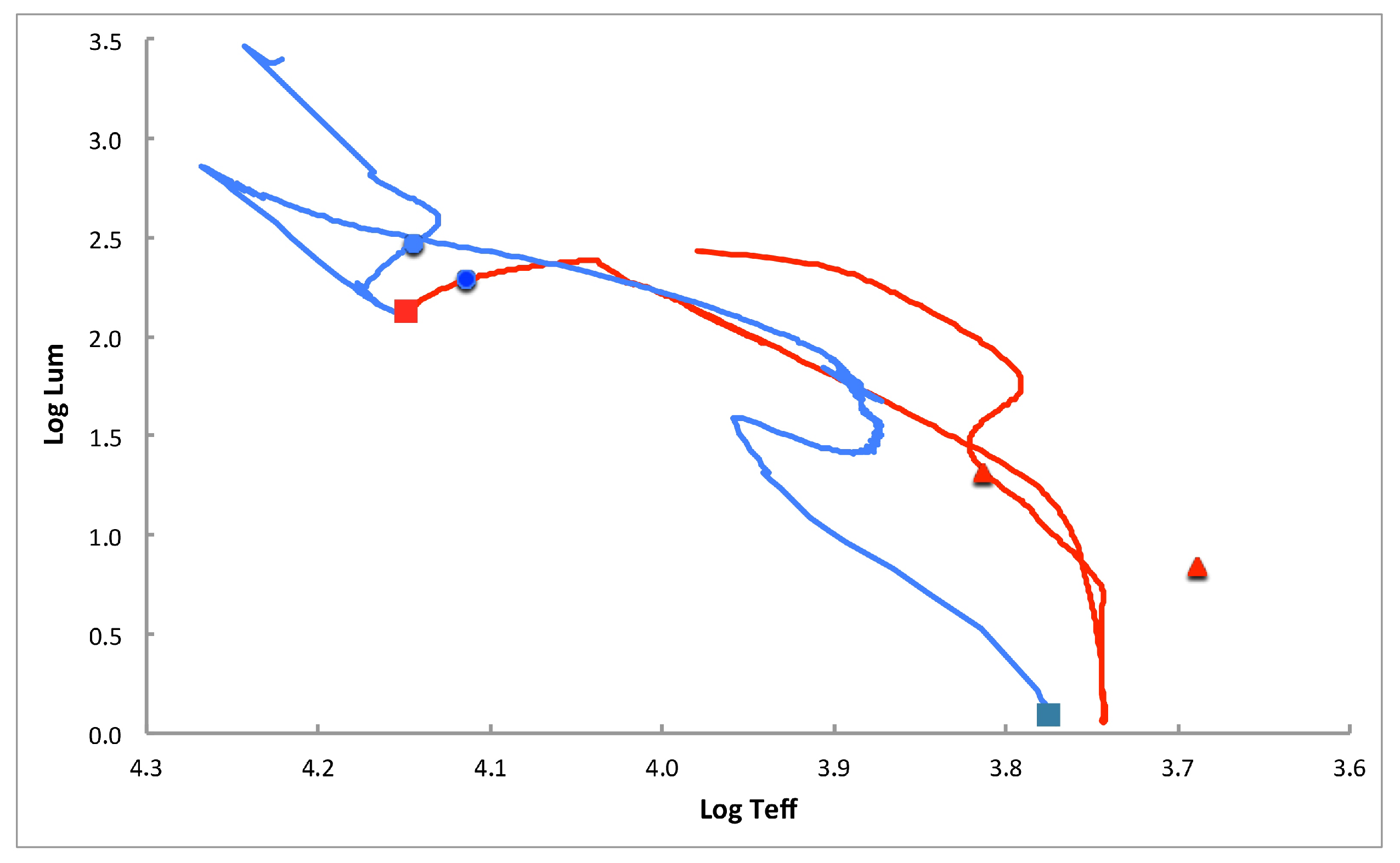
Every observed binary has a large number of possible progenitors with different values for their masses and different initial periods. Our evolution code recognizes a progenitor as plausible when the calculated positions of donor and gainer in the HRD are found to be close to the observations. The HRD is an effective temperature-luminosity diagram. Observers refer to it as colour -magnitude diagram (abbreviated as CMD). As an example, Figure 1 shows the evolutionary path of $\beta$ Per: prototype of the Algol-type binaries. The present characteristics of Algol are from the catalogue of Budding et al. [16]. All characteristics have been accurately retrieved by our code, except the T${}_{\mathrm{eff}}$-values. However, Zavala et al. [17] revised these T${}_{\mathrm{eff}}$-values. Their value of T${}_{\mathrm{eff}}$ for the gainer is closely approximated by our calculations. The progenitor is a ($3.41{\mathrm{M}}_{\odot }+1.1{\mathrm{M}}_{\odot }$) binary with an initial period of 1.4625 days. This binary lives two eras of RLOF. Nowadays, the second era of RLOF (RLOF B during H-shell burning of the donor) is at work. Figure 1 shows that the observed location of the gainer is produced by the calculations, whereas the calculated effective temperature of the donor remains larger than the observed one, as mentioned in the catalogue of Budding et al. [16]. Figure 1 also shows the locations on the Zero Age Main Sequence, where both stars start their life. During evolution, the originally most massive donor becomes the less massive member of the binary. Presently, the most massive gainer is still on the Main Sequence (abbreviated as MS) of the HRD, whereas the less massive donor has evolved far away from the MS. The Algol paradox states that the most massive member of an Algol-binary is less evolved than his less massive companion. Figure 1 shows the well-known solution to this paradox.

3. Tidal Interaction

Neglecting tides and magnetic braking, Packet [18] showed that mass gainers continue to rotate with the critical velocity after the accretion of only 5% to 10% of their own mass. This critical velocity is, in most cases, much faster than that observed. Van Rensbergen et al. [11] calculated a grid of evolutionary tracks with a simple approach for tidal interaction and the possibility for binaries to live through liberal eras during their evolution.

Darwin [19] developed tidal interaction as first. Tides act on both stars of the binary, depending on their radius “R” and the semi major axis “a” of the binary orbit. A typical synchronization time is given by:

$${\tau }_{\mathrm{sync}}={\mathrm{q}}^{-2}{\left(\frac{\mathrm{a}}{\mathrm{R}}\right)}^6$$

(1)

The mass of the star undergoing the tide is in the denominator of the mass ratio $\mathrm{q}$ in Equation (1). Tides tend to synchronize the angular velocities of the stellar rotation ($\Omega$) with the angular velocity of the orbit (${\Omega }_{\mathrm{orb}}$), as shown in Equation (4).

In order to distinguish strong tides from weak tides, Wellstein [20] proposed calculating the synchronization time with:

$${\mathrm{t}}_{\mathrm{sync}}={\tau }_{\mathrm{sync}}{\mathrm{f}}_{\mathrm{sync}}$$

(2)

For strong tides, Wellstein [20] uses ${\mathrm{f}}_{\mathrm{sync}}$ = 0.1, for weak tides ${\mathrm{f}}_{\mathrm{sync}}$ = 1 is taken in Equation (2). Both of the values of ${\mathrm{f}}_{\mathrm{sync}}$ were used by Van Rensbergen & De Greve et al. [11,12,13]. Strong tides should be preferred over weak tides in order to obtain a better agreement between observed and calculated distributions of mass ratios an orbital periods. Nevertheless, strong tides are also not able to predict the population of Algol-binaries with the smallest observed orbital periods.

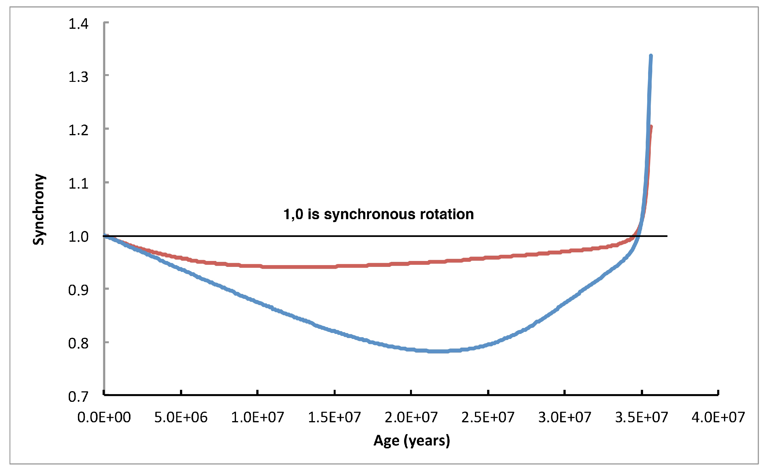
In order to avoid the random number ${\mathrm{f}}_{\mathrm{sync}}$, Van Rensbergen & De Greve [14] calculated ${\mathrm{t}}_{\mathrm{sync}}$ with a physical model, distinguishing convective from radiative envelopes. Hurley et al. [21] use an expression of Hut [22] to calculate ${\mathrm{t}}_{\mathrm{sync}}$ for a star with a convective envelope. Hilditch [23] gives an expression of Zahn [24] to calculate the tidal action on a star with radiative envelope. In the following, we will designate these synchronization times with ${\mathrm{t}}_{\mathrm{sync},\mathrm{Darwin}}$. Assuming that mass accretion causes turbulence in the atmosphere, the convective mode was always applied during RLOF. Meridional circulation, as proposed by Tassoul [25], was added as a significant contributor to tidal interaction. Figure 2 shows the effect of Tassoul’s mechanism, presenting the degree of synchronism of the 8 ${\mathrm{M}}_{\odot }$ star in a (8 ${\mathrm{M}}_{\odot }$ + 3 ${\mathrm{M}}_{\odot }$)-system in the pre-RLOF phase. During RLOF, the separation of different tidal effects is blurred by the mass transfer.

Thus, the tidal synchronization time was calculated with:

$$\frac{1}{{\mathrm{t}}_{\mathrm{sync}}}=\frac{1}{{\mathrm{t}}_{\mathrm{sync},\mathrm{Darwin}}}+\frac{1}{{\mathrm{t}}_{\mathrm{sync},\mathrm{Tassoul}}}$$

(3)

Tidal synchronization tries to equalize the angular velocities of the stars ($\Omega$) in a binary with angular velocity (${\Omega }_{\mathrm{orb}}$) of orbital rotation. Because of tides, a rotating star with moment of inertia I and angular velocity $\Omega$ will change its spin angular momentum by an amount

$$\Delta {\mathrm{J}}_{\mathrm{spin}}=\mathrm{I}\left({\Omega }_{\mathrm{orb}}-\Omega \right)\left(1-{\mathrm{e}}^{\frac{\Delta t}{{\mathrm{t}}_{\mathrm{sync}}}}\right)$$

(4)

This equation shows that tides cease their action on the rotation of a star when synchronism is achieved with $\Omega ={\Omega }_{\mathrm{orb}}$.

4. Liberal Evolution

Peters & Polidan [26] introduced the concept of hot spots (also called HTAR: High Temperature Accretion Regions) that are created at the trailing side of the gainer by the mass-transfer from the donor hitting the gainer star. Van Rensbergen & De Greve [12,13] used these hot spots to act together with rapid rotation of the gainer, attempting to surpass the binding energy at the HTAR-location. More massive binaries reach that condition, as they yield both characteristics, fast rotation and a very hot spot, during periods of rapid mass transfer. The evolution of the binary will be liberal during such an era. The influence of liberal evolution on the distribution of orbital periods and mass ratios of the evolutionary models was compared to the observed distributions for 351 Algols, which were taken from the catalogue of Budding et al. [16]. This catalogue uses different values of the mass ratio: ${\mathrm{q}}_{\mathrm{LC}}$ is the mass ratio that is derived with the light curve solution and ${\mathrm{q}}_{\mathrm{MS}}$ is the mass ratio derived to make the parameters of the gainer stars to fit Main Sequence characteristics.

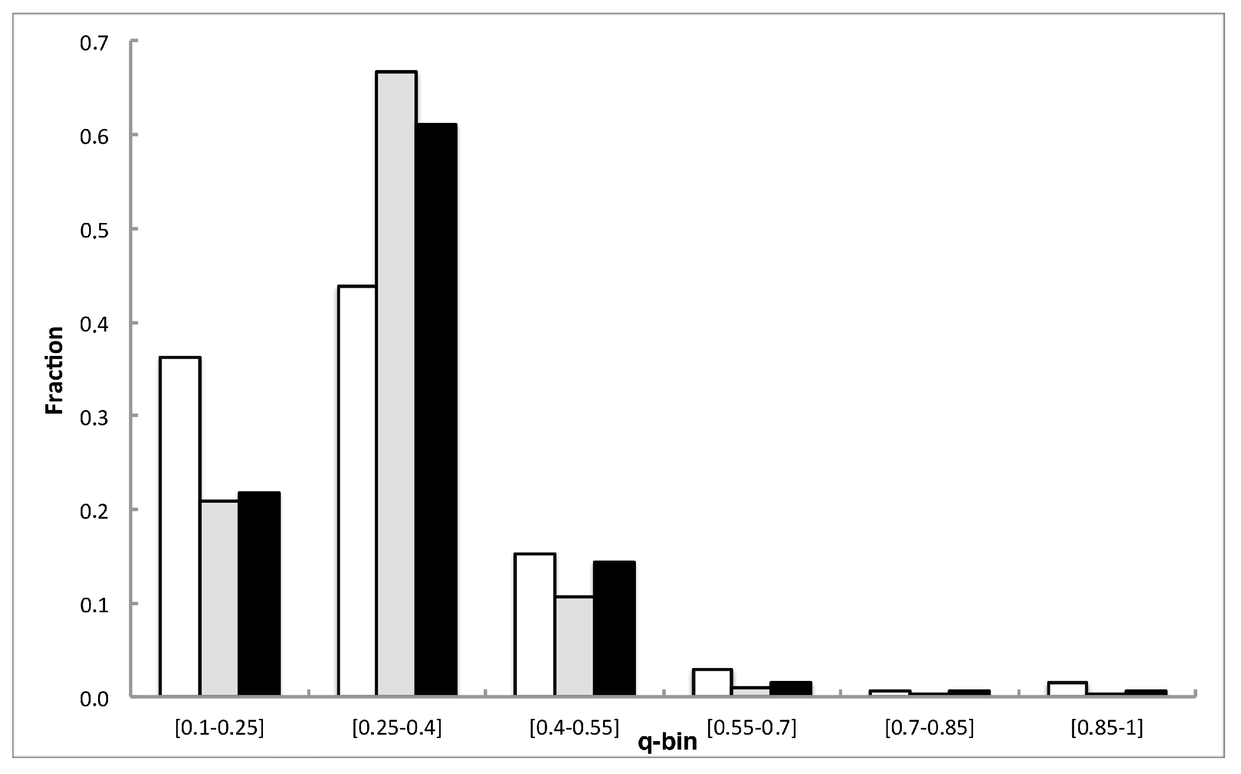
Figure 3 compares observations and our models for the mass ratio distribution q = $\frac{{\mathrm{M}}_{\mathrm{d}}}{{\mathrm{M}}_{\mathrm{g}}}$, where the subscript “d” is used for the donor star and “g” for the gainer. We updated the comparison by taking the quantity ${\mathrm{q}}_{\mathrm{LC}}$ for the observed distribution instead of ${\mathrm{q}}_{\mathrm{MS}}$, as the latter value results in larger uncertainties than the former. The agreement between observations and model is better than satisfactory, as compared to the result that was obtained by Van Rensbergen et al. [13], with the injudicious use of ${\mathrm{q}}_{\mathrm{MS}}$, which produces too many Algols with large mass ratios, a result that is contradicted by observations. The majority of Algols, having lower mass progenitors, evolve conservatively. The less numerous more massive Algols evolve very differently as a consequence of their liberal eras. However, since most Algols evolve conservatively, conservative and liberal simulations yield similar distributions of the mass ratio.

The initial conditions for the simulations are from Salpeter [27] for the Initial Mass Function (IMF) of the future donor, from Van Rensbergen et al. [28] for the initial mass ratio distribution, and from Popova et al. [29] for the distribution of the initial orbital periods.

Figure 4 shows that the observed distribution of orbital periods of 376 Algols from the catalogue of Budding et al. [16] is well reproduced by our simulation. The difference of 376 with the earlier mentioned 351 comes from the fact that the period is known for 25 systems, for which the mass ratio still remains to be determined. In this case there is no difference between the results obtained from the conservative and the liberal simulation. However, our simulations yield almost no Algols with orbital periods shorter than one day, in contrast with the ≈10 % found in the catalogue.

5. Magnetic Braking

Tides and liberal evolution cannot explain the observed rotational velocities of the mass gainers published by Van Hamme and Wilson [30], Miller et al. [31], Glazunova et al. [32], and Dervisoglu et al. [33]. Therefore, we investigated another possible process. In Section 5.1 we explain how to calculate the magnetic field strength, while using a simple model of differential rotation. The resulting magnetic braking rises with increasing values of the magnetic field and the amount of mass loss through stellar wind. The mass losses by stellar wind are from Vink et al. [34] for stars hotter than 12,500 K and De Jager et al. [35] for cooler stars. Details of the calculation method can be found in Van Rensbergen & De Greve [15]. We further report the results, including magnetic braking, in order to better understand the observed rotational velocities of Algol-type systems.

5.1. Generation of the Magnetic Field of the Gainer

A solid body rotator with constant angular velocity $\Omega$ from the centre to the edge of the star cannot develop a magnetic field. We use a model, wherein only the outer shell is spun up by the mass-transfer from the donor hitting the gainer. During rapid RLOF the outer shell rotates faster than the core of the gainer whose rotation is not accelerated. The magnetic fields that are produced by the dynamo model of Spruit [36] are at work when the angular velocity increases with an amount $\Delta \Omega$ over a distance $\Delta$r. Packet [18] only gives the amount of angular momentum that is added to the shell, being reduced by the quotient of the impact-parameter d over the radius of the gainer ${\mathrm{R}}_{\mathrm{g}}$ (rendering the spin-up inefficient at close approach):

$$\Delta {\mathrm{J}}_{\mathrm{spin},\mathrm{shell}}^{+}=6.04534{10}^{54}{\mathrm{R}}_{\mathrm{g}}{\left({\mathrm{M}}_{\mathrm{g}}+\frac{\Delta {\mathrm{M}}_{\mathrm{g}}}{2}\right)}^{\frac{1}{2}}\left(\frac{\mathrm{d}}{{\mathrm{R}}_{\mathrm{g}}}\right)$$

(5)

$\Delta {\mathrm{J}}_{\mathrm{spin},\mathrm{shell}}^{+}$ is expressed in cgs units, whereas masses and radii are, respectively, in ${\mathrm{M}}_{\odot }$ and ${\mathrm{R}}_{\odot }$.

With every value of ${\mathrm{J}}_{\mathrm{spin},\mathrm{shell}}$ corresponds a value of ${\Omega }_{\mathrm{shell}}$=$\frac{{\mathrm{J}}_{\mathrm{spin},\mathrm{shell}}}{{\mathrm{I}}_{\mathrm{shell}}}$, which is a characteristic value of the angular velocity in the shell. A magnetic field is created when ${\Omega }_{\mathrm{shell}}$ > ${\Omega }_{\mathrm{core}}$. However, the value of $\Omega$ cannot change discontinuously from ${\Omega }_{\mathrm{core}}$ to ${\Omega }_{\mathrm{shell}}$ at the interface between core and shell. In order to accomplish the continuity of $\Omega$(r) and to avoid friction between the outer edge of the core and the inner surface of the shell, we chose a radius-dependent angular velocity $\Omega$(r) continuously increasing from ${\Omega }_{\mathrm{core}}$ at the interface between core and shell to ${\Omega }_{\mathrm{edge}}$ at the edge of the gainer.

5.2. Extent of the Shell

The gainer is now composed of an inner core in solid rotation that was surrounded by a shell that rotates differentially. The core is not spun up or slowed down magnetically. Its rotation is only modulated by tides. When the shell is spun up following relation (5), the spin-down follows relation (4).

A core with a core fraction CF of the mass of the gainer leaves (1-CF) for the mass for the shell.

Figure 5 shows the evolution with time of the equatorial velocity of the gainer starting from a (6.36 + 2.7) ${\mathrm{M}}_{\odot }$ binary with an initial orbital period of 1.89745 d. This is a plausible progenitor for $\lambda$ Tau, although any other binary in our collection of calculated cases could have been chosen to illustrate our updated binary evolutionary scenario. The calculation was performed for the system undergoing tides and magnetic braking with an initial value of CF = 0.95. The evolution with time is compared with the evolution of the gainer in the same system with a rigidly rotating and, hence, never magnetic gainer, for which the rotation is only affected by tides. Also included in the figure is the evolution when neither tides nor magnetic braking are active, showing that, in the latter case, the gainer remains rotating with critical velocity once this velocity is achieved. The plausible progenitor for $\lambda$ Tau starts RLOF during core hydrogen burning of the donor (RLOF A). A critical rotation of the gainer is achieved during this phase of rapid RLOF at ≈48 million years after ZAMS. After that, RLOF A occurs at a lower speed. Tidal interaction and magnetic braking are then strong enough to synchronize the rotation of the gainer. In Figure 5, one clearly sees that synchronization settles more rapidly when magnetic braking helps tidal interaction. After ≈65 million years, during hydrogen shell burning of the donor, RLOF restarts. Critical rotation is again attained. However, the rush to critical rotation is slowed down by the combined action of tides and magnetic braking. The present observed state of $\lambda$ Tau occurs during this stage of rising rotational velocity. The gainer of $\lambda$ Tau now has an equatorial velocity that is far below the critical value.

When critical rotation is achieved during RLOF B, the orbital period is ≈30 days. Figure 5 shows that tides are then too weak to prevent critical rotation. However, magnetic braking will decrease the velocity below the critical value. This happens at the very end of, and after, RLOF B.

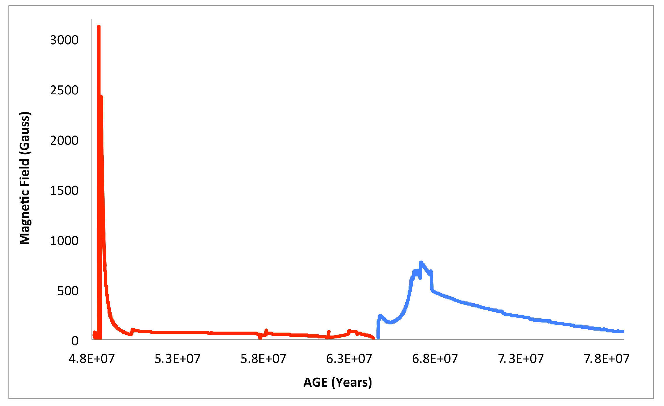
Figure 6 shows the evolution of the magnetic field of the gainer in the binary that is shown in Figure 5. Before RLOF A, the shell and core of the gainer have the same synchronous rotational velocity. The core always continues to rotate almost synchronously. When RLOF A starts, only the shell is spun up. When the shell rotates at critical velocity, the magnetic field is at a maximum of ≈3000 Gauss for a short time. The magnetic field disappears when tides and magnetic braking have synchronized the rotation of the shell. From the beginning of RLOF B, the shell is again spun up, and the magnetic field starts to be built up again. The value of the magnetic field is lower than during rapid RLOF A. A value of ≈750 Gauss is reached. The magnetic braking is then still sufficiently active to synchronize the shell. After that, the magnetic field disappears again.

6. Calculated Cases

Van Hamme & Wilson [30] defined the quantity F=$\frac{{\mathrm{v}}_{\mathrm{eq}}}{{\mathrm{v}}_{\mathrm{sync}}}$: the ratio between the equatorial velocity ${\mathrm{v}}_{\mathrm{eq}}$ and the synchronous velocity ${\mathrm{v}}_{\mathrm{sync}}$. Subsequently, they determined R=$\frac{{\mathrm{F}}_{\mathrm{gainer}}-1}{{\mathrm{F}}_{\mathrm{crit},\mathrm{gainer}}-1}$. This quantity R ∈ [0–1] is a measure of rotation. Specifically, R is 0 at synchronous rotation and 1 at critical rotation. The use of the quantity R as a characteristic measure of rotation has the advantage that minor differences in the evaluation of the synchronous and critical velocities by different authors are ironed out. A determination of ${\mathrm{v}}_{\mathrm{eq}}$ is considered to be good when $\Delta$R = |${\mathrm{R}}_{\mathrm{model}}-{\mathrm{R}}_{\mathrm{obs}}$| is small (near to 0) and it is unacceptable when the same quantity is large (close to 1). We found 41 Algol-type binaries for which the equatorial velocity of the gainer was published. These systems are shown in

Table 1. Calculated equatorial velocities of gainers that best fit observations. Masses are in ${\mathrm{M}}_{\odot }$, orbital periods in days and ${\mathrm{v}}_{\mathrm{eq}}$ in $\frac{\mathrm{km}}{\sec }$. For each system, two lines are given, the first with data from observations and the second with the results from the model. The masses mentioned by the observations of Glazunova et al. [32] are from Budding et al. ([16]).

System	${\mathbf{M}}_{\mathbf{gainer}}$ obs	${\mathbf{M}}_{\mathbf{donor}}$ obs	${\mathbf{v}}_{\mathbf{eq}}$ obs	R obs	Reference-Observations
Progenitor	${\mathbf{M}}_{\mathbf{gainer}}$ calc	${\mathbf{M}}_{\mathbf{donor}}$ calc	${\mathbf{v}}_{\mathbf{eq}}$ calc	R calc	Initial Period Progenitor
		Very good	Agreement	$\Delta$R ≤ 0.1
$\beta$ Per	3.70	0.81	52.51	0.00	Dervisoglu et al. [33]
3.41 + 1.1	3.69	0.82	50.04	0.00	1.146250
HS Hya	2.47	0.70	45.41	0.01	Glazunova et al. [32]
2.37 + 0.8	2.47	0.70	78.97	0.00	1.18912
KO Aql	2.53	0.55	41.92	0.02	Dervisoglu et al. [33]
2.28 + 0.8	2.53	0.55	50.33	0.01	1.27150
CW Eri	2.59	0.74	33.28	−0.01	Glazunova et al. [32]
2.23 + 1.1	2.59	0.74	48.22	0.01	1.30138
ZZ Boo	3.43	0.96	9.51	−0.02	Glazunova et al. [32]
2.59 + 1,8	3.49	0.90	48.19	0.01	1.5
AU Mon	5.93	1.18	126.32	0.25	Dervisoglu et al. [33]
4.16 + 3.00	5.93	1.19	104.87	0.22	2.005
Y Psc	2.80	0.70	38.05	0.00	Dervisoglu et al. [33]
2.3 + 1,2	2.80	0.70	47.58	0.03	1.34865
WW Cyg	2.10	0.60	41.01	0.03	Dervisoglu et al. [33]
1.5 + 1.2	2.10	0.60	51.35	0.06	1.138
V505 Sgr	2.68	1.23	102.56	0.05	Dervisoglu et al. [33]
2.71 + 1.2	2.67	1.24	107.85	0.08	1.23198
TX UMa	4.76	1.18	63.62	0.04	Dervisoglu et al. [33]
4.24 + 1.7	4.75	1.19	71.78	0.00	1.44948
XY Cet	5.30	0.94	84.05	0.07	Glazunova et al. [32]
5.04 + 1.2	5.09	1.14	72.46	0.02	1.55429
SZ Psc	3.00	0.77	9.26	−0.03	Glazunova et al. [32]
2.47 + 1.3	3.00	0.77	44.38	0.03	1.4765
RZ Cas	2.10	0.74	87.65	0.06	Dervisoglu et al. [33]
2.14 + 0.7	2.10	0.74	62.93	0.00	1.33437
U Cep	3.57	1.86	437.37	0.87	Dervisoglu et al. [33]
3.33 + 2.1	3.56	1.87	488.95	0.95	2.13447
UV Psc	1.86	0.77	70.81	0.01	Glazunova et al. [32]
2.03 + 0.6	1.86	0.77	105.78	−0.09	1.3999
AI Dra	2.37	1.09	86.90	−0.06	Van Hamme & Wilson [30]
2.36 + 1.1	2.36	1.10	85.71	0.04	1.18128
		Good	Agreement	$\Delta$R ∈ [0.11–0.35]
CD Tau	2.5	1.0	20.91	0.00	Glazunova et al. [32]
1.9 + 1.6	2.5	1.0	77.27	0.11	1.91047
AT Peg	2.50	1.21	84.51	0.01	Dervisoglu et al. [33]
2.61 + 1.1	2.49	1.22	121.86	0.12	1.3406
TV Cas	3.78	1.53	80.48	−0.03	Dervisoglu et al. [33]
3.21 + 2.1	3.77	1.54	117.86	0.12	1.14467
RW Tau	2.43	0.55	94.00	0.18	Van Hamme & Wilson [30]
2.18 + 0.8	2.43	0.55	50.13	0.02	1.24613
VZ Hya	2.52	0.89	19.90	0.00	Glazunova et al. [32]
2.01 + 1.4	2.52	0.89	107.24	0.17	1.47042
X Tri	2.43	1.21	50.00	−0.16	Van Hamme & Wilson [30]
2.44 + 1.2	2.43	1.21	93.42	0.02	0.98383
Z Vul	5.39	2.26	135.02	0.18	Van Hamme & Wilson [30]
5.65 + 2.0	5.36	2.28	142.71	0.00	3.07536
IM Aur	2.38	0.77	139,76	0.20	Van Hamme & Wilson [30]
2.35 + 0.8	2.38	0.77	70.04	0.00	1.15531

and

Table 2. Calculated equatorial velocities of gainers fitting observations less good than in Table 1. The masses for V356 Sgr are from ([37]). There are no systems found with $\Delta$R ∈ [0.36–0.49].

System	${\mathbf{M}}_{\mathbf{gainer}}$ obs	${\mathbf{M}}_{\mathbf{donor}}$ obs	${\mathbf{v}}_{\mathbf{eq}}$ obs	R obs	Reference-Observations
Progenitor	${\mathbf{M}}_{\mathbf{gainer}}$ calc	${\mathbf{M}}_{\mathbf{donor}}$ calc	${\mathbf{v}}_{\mathbf{eq}}$ calc	R calc	Initial Period Progenitor
		Good	Agreement (continued)	$\Delta$R ∈ [0.11–0.35]
DL Vir	2.18	1.06	121.00	0.20	Van Hamme & Wilson [30]
2.44 + 0.8	2.17	1.07	136.81	0.00	2.18242
$\delta$ Lib	4.76	1.67	68.85	−0.09	Van Hamme & Wilson [30]
3.93 + 2.5	4.75	1.69	113.16	0.12	1.23263
$\lambda$ Tau	7.19	1.87	90.96	0.05	Van Hamme & Wilson [30]
6.36 + 2.7	7.15	1.88	177.83	0.26	1.89745
V356 Sgr	10.40	2.80	212,81	0.37	Glazunova et al. [32]
8.7 + 6	10.90	2.64	118.34	0.14	1.86560
TW Dra	1.70	0.80	37.09	−0.02	Dervisoglu et al. [33]
1.5 + 1.0	1.70	0.80	121.51	0.23	2.092
RX Gem	4.40	0.80	157.60	0.38	Dervisoglu et al. [33]
3.0 + 2.2	4.40	0.80	298.59	0.69	1.85226
TW And	1.68	0.32	31.64	0.01	Glazunova et al. [32]
1.4 + 0.6	1.68	0.32	155.42	0.32	1.08976
W Del	2.01	0.42	30.00	0.03	Van Hamme & Wilson [30]
1.53 + 0.9	2.01	0.42	169.80	0.36	1.10746
SW Cyg	2.50	0.50	197.47	0.46	Dervisoglu et al. [33]
2.1 + 0.9	2.50	0.50	73.25	0.13	1.32299
		Weak	Agreement	$\Delta$R ∈ [0.5–0.90]
TT Hya	2.77	0.63	168.93	0.44	Miller et al. ([31])
2.0 + 1.4	2.77	0.63	482.24	1.00	1.68341
RY Per	6.24	1.69	214.60	0.39	Dervisoglu et al. [33]
4.45 + 3.40	6.22	1.63	556.23	0.99	1.98167
RS Cep	2.83	0.41	170.23	0.33	Dervisoglu et al. [33]
2.04 + 1.2	2.83	0.41	412.17	0.99	1.32215
AD Her	2.90	0.90	143.79	0.31	Dervisoglu et al. [33]
2.7 + 1.1	2.90	0.91	382.61	1.00	6.6282
RY Gem	2.66	0.24	70.53	0.14	Glazunova et al. [32]
2.35 + 0.55	2.61	0.24	376.12	0.87	1.12077
TU Mon	12.6	2.7	153.02	0.18	Dervisoglu et al. [33]
11.5 + 4.3	12.09	2.74	621.52	0.98	1.75065
U Sge	4.45	1.65	76.00	0.04	Dervisoglu et al. [33]
3.4 + 2.7	4.44	1.66	446.87	0.86	1.72982
		No	Agreement	$\Delta$R > 0.90
U CrB	6.78	2.87	60.59	0.04	Van Hamme & Wilson [30]
5.25 + 4.4	6.76	2.88	533.20	0.99	2.06346

, running from $\Delta$R = 0 at the top of Table 1 to the bottom of Table 2 where $\Delta$R ≈ 1. The Tables show two lines for each system (first line: observed data; second line: data from the model), showing that:

• The observed equatorial velocities of 16 Algol-systems are very well confirmed by theory ($\Delta$R < 0.1).
• Seventeen more Algols can be considered andl explained by the theory ($\Delta$R ∈ [0.11–0.35]).
• No systems were found with $\Delta$R ∈ [0.36–0.49].
• Seven other Algol-systems are weakly reproduced by the theory ($\Delta$R ∈ [0.50–0.90]).
• Only one Algol (U CrB) is badly reproduced by the theory ($\Delta$R > 0.90).

7. Conclusions

For a large part of Algol-type binaries with well observed characteristics, fairly accurate models can be calculated matching the present position in the HRD. For some systems, a better determination of fundamental parameters, such as T${}_{\mathrm{eff}}$ for the cooler donor star is needed. The observed distributions of mass ratios and orbital periods of Algol-type binaries are reasonably well reproduced by our models, although additional work is needed to represent the very short period Algols, as can be seen in Figure 3 and Figure 4. We suggest shedding new light on the contact phase evolution, where very short orbital periods are the rule. The present calculations show that magnetic braking added to tidal interaction clearly helps to reduce the rotational equatorial velocity of the gainer star, away from the critical one. Reasonable to good agreement between the observed and calculated rotational velocities was obtained for 33 out of 41 gainers in Algol-type binaries. The unsatisfying result for eight systems requires further investigation. It may be due to different causes. The current period is well known, but that is not the case for the masses. If future analysis would deliver other values for the observed masses, then this would result in different progenitors, subsequently with a different ${\mathrm{v}}_{\mathrm{eq}}$-evolution. Additionally, the eight systems all occur long after the minimum period (late case A or case B). A new approach towards their previous contact phase may also produce different results. Our models predict that Algol-type binaries may show a strong magnetic field for a short time during phases of rapid mass transfer.

References

- Paczynski, B. Evolution of Close Binaries I. Acta Astron. 1966, 16, 231–247. [Google Scholar]
- Paczynski, B. Evolution of Close Binaries IV. Acta Astron. 1967, 17, 193–206. [Google Scholar]
- Paczynski, B. Evolution of Close Binaries V. Acta Astron. 1967, 17, 355–378. [Google Scholar]
- Kippenhahn, R.; Weigert, A. Entwicklung in engen Doppelsternsystemen I. ZA 1967, 65, 251–273. [Google Scholar]
- Tutukov, A.; Yungelson, L. Evolution of close binaries with mass loss from the system. Nauchnye Informatsii 1971, 20, 86–93. [Google Scholar]
- Tutukov, A. Evolution of Close Binaries. In Fundamental Problems in the Theory of Stellar Evolution, Proceedings of the Symposium, Kyoto, Japan, 22–25 July 1980; Reidel Publishing Co.: Dordrecht, The Netherlands, 1981; pp. 137–153. [Google Scholar]
- Eggleton, P. Evolutionary Processes in Binary and Multiple Stars, 1st ed.; Cambridge University Press: Cambridge, UK, 2001. [Google Scholar]
- Nelson, C.; Eggleton, P. A Complete Survey of Case A Binary Evolution with Comparison to Observed Algol-type Systems. Astrophys. J. 2001, 552, 664–678. [Google Scholar] [CrossRef] [Green Version]
- Song, H.; Maeder, A.; Meynet, G.; Huang, Q.; Ekström, S.; Granada, A. Close-binary evolution I. Astron. Astrophys. 2013, 556, A100. [Google Scholar] [CrossRef]
- Song, H.; Meynet, G.; Maeder, A.; Ekström, S.; Eggenberger, P.; Georgy, C.; Qin, Y.; Fragos, T.; Soerensen, M.; Barblan, F.; et al. Close-binary evolution II. Astron. Astrophys. 2018, 609, A3. [Google Scholar] [CrossRef] [Green Version]
- Van Rensbergen, W.; De Greve, J.P.; De Loore, C.; Mennekens, N. Spin-up and hot spots can drive mass out of a binary. Astron. Astrophys. 2008, 487, 1129–1138. [Google Scholar] [CrossRef] [Green Version]
- Van Rensbergen, W.; De Greve, J.P.; Mennekens, N.; Jansen, K.; De Loore, C. Mass loss out of close binaries. Case A Roche lobe overflow. Astron. Astrophys. 2010, 510, A13. [Google Scholar] [CrossRef] [Green Version]
- Van Rensbergen, W.; De Greve, J.P.; Mennekens, N.; Jansen, K.; De Loore, C. Mass loss out of close binaries. The formation of Algol-type systems completed with case B RLOF. Astron. Astrophys. 2011, 528, A16. [Google Scholar] [CrossRef] [Green Version]
- Van Rensbergen, W.; De Greve, J.P. Accretion disks in Algols, Progenitors and evolution. Astron. Astrophys. 2016, 592, A151. [Google Scholar] [CrossRef] [Green Version]
- Van Rensbergen, W.; De Greve, J.P. Magnetic braking at work in binaries. Astron. Astrophys. 2020, 642, A183. [Google Scholar] [CrossRef]
- Budding, E.; Erdem, A.; Cicek, C.; Bulut, I.; Soydugan, F.; Soydugan, E.; Bakis, V.; Demircan, O. Catalogue of Algol type binary stars. Astron. Astrophys. 2004, 417, 263–268. [Google Scholar] [CrossRef]
- Zavala, R.; Hummel, C.; Boboltz, D.; Ojha, R.; Shaffer, D.; Tycner, C.; Richards, M.; Hutter, D. The Algol Triple System Spatially resolved at Optical Wavelengths. Astrophys. J. Lett. 2010, 715, L18, Erratum in 2017, 843, L44. [Google Scholar] [CrossRef] [Green Version]
- Packet, P. On the spin-up of the Mass Accreting Component in a Close Binary System. Astron. Astrophys. 1981, 102, 17–19. [Google Scholar]
- Darwin, G. On the Secular Changes in the Elements of the Orbit of a Satellite Revolving about a Tidally Distorted Planet. Philos. Trans. R. Soc. Lond. 1880, 171, 713–891. [Google Scholar]
- Wellstein, S. Präsupernovaentwicklung Enger Massereicher Doppelsternsysteme. Ph.D. Thesis, Potsdam University, Potsdam, Germany, 2001. [Google Scholar]
- Hurley, J.; Tout, C.; Pols, O. Evolution of binary stars and the effect of tides on binary populations. Mon. Not. R. Astron. Soc. MNRS 2002, 329, 897–928. [Google Scholar] [CrossRef]
- Hut, P. Tidal evolution in close binary systems. Astron. Astrophys. 1981, 99, 126–140. [Google Scholar]
- Hilditch, R. An Introduction to Close Binary Stars; Cambridge University Press: Cambridge, UK, 2001; pp. 152–154. [Google Scholar]
- Zahn, J.P. Tidal Friction in Close Binary Stars. Astron. Astrophys. 1977, 57, 383–394. [Google Scholar]
- Tassoul, J.L. Stellar Rotation; Cambridge University Press: Cambridge, UK, 2000; pp. 214–228. [Google Scholar]
- Peters, G.; Polidan, R. Evidence for a high temperature accretion region in Algol-type binary systems. Astrophys. J. 1984, 283, 745–759. [Google Scholar] [CrossRef]
- Salpeter, E. The Luminosity Function and Stellar Evolution. Astrophys. J. 1955, 121, 161–167. [Google Scholar] [CrossRef]
- Van Rensbergen, W.; De Loore, C.; Jansen, K. Evolution of interacting binaries with a B type primary at birth. Astron. Astrophys. 2006, 446, 1071–1079. [Google Scholar] [CrossRef] [Green Version]
- Popova, E.; Tutukov, A.; Yungelson, L. Study of Physical Properties of Spectroscopic Binary Stars. Astrophys. Space Sci. 1982, 88, 55–80. [Google Scholar] [CrossRef]
- Van Hamme, W.; Wilson, R. Rotation Statistics of Algol-type binaries and Results on RY Geminorum, RW Monocerotis and RW Tauri. Astron. J. 1990, 100, 1982–1993. [Google Scholar] [CrossRef]
- Miller, B.; Budaj, J.; Richards, M. Revealing the Nature of Algol Disks through Optical and UV Spectroscopy, Synthetic Spectra and Tomography of TT Hya. Astrophys. J. 2007, 656, 1075–1091. [Google Scholar] [CrossRef] [Green Version]
- Glazunova, L.; Yushcenko, A.; Tsymbal, V.; Mkrtichian, D.; Lee, J.; Kang, Y.; Valyavin, G.; Lee, B. Rotational Velocities of the Components of 23 Binaries. Astrophys. J. 2008, 135, 1736–1745. [Google Scholar] [CrossRef] [Green Version]
- Dervisoglu, A.; Tout, C.; Ibanglu, C. Spin angular momentum evolution of the long-period Algols. Mon. Not. R. Astron. Soc. MNRS 2010, 406, 1071–1083. [Google Scholar]
- Vink, J.; De Koter, A.; Lamers, H. Mass-loss predictions for O and B stars as a function of metallicity. Astron. Astrophys. 2001, 369, 574–588. [Google Scholar] [CrossRef]
- De Jager, C.; Nieuwenhuyzen, H.; Van der Hucht, K. Mass Loss Rates in the Hertzsprung-Russell Diagram. Astron. Astrophys. Suppl. Ser. 1988, 72, 259–289. [Google Scholar]
- Spruit, H. Dynamo action of differential rotation in a stably stratified stellar interior. Astron. Astrophys. 2002, 381, 923–932. [Google Scholar] [CrossRef] [Green Version]
- Dominis, D.; Mimica, P.; Pavlovski, K.; Tamajo, E. In between β Lyrae and Algol: The Case Of V356 Sgr. ApSS 2005, 296, 189–192. [Google Scholar]
Figure 1.
Hertzsprung Russell diagram (HRD) evolution of Per. Starting at the red square, the donor follows the red path (observed and calculated positions: triangles). Starting at the blue square, the gainer follows the blue path close to the Main Sequence (observed and calculated positions: filled circles).
Figure 2.
Deviation from synchronous rotation of a 8 -primary caused by tidal interaction with its 3 -companion. The blue line illustrates the action of the Darwin mechanism. The addition of the Tassoul mechanism to synchronization is shown by the red line.
Figure 3.
The observed distribution of the mass ratio for 351 Algols (white) as compared to conservative (grey) and liberal (black) simulation.
Figure 4.
Observed distribution of orbital periods for 376 Algols (grey) as compared to simulation (black).
Figure 5.
Evolution with age of the equatorial velocity of the gainer of a () binary with an initial period of 1.89745 days. Black line: tides and magnetic braking are not at work; red line: tides act alone; blue line: tides and magnetic braking act together.
Figure 6.
Evolution of the radial magnetic field strength (in Gauss) produced by the Spruit mechanism for the binary mentioned in Figure 5. (Case A: red; Case B: blue).