An Unofficial Account of the Beginnings of VLBI Polarimetry: From Jodrell Bank to the Event Horizon Telescope

Abstract

I offer a brief and personal history of the development of polarization sensitive observations with widely separated antennas. The story starts at Jodrell Bank in the late 1960s with a 24 km baseline radio linked (but not phase stable) interferometer and reaches to the present Event Horizon Telescope (with global span and independent atomic clocks) which has just published an image of the linearly polarized radiation surrounding the black hole shadow of M87*. I was privileged to be witness to many of the developments along the way, either as an instigator, a bystander, or an unindicted co-conspirator. I am most interested in the technical developments that enabled these increasingly sophisticated observations, and in the ideas that advanced the data analysis and imaging.

1. Introduction

This is a story about radio astronomy. It is about the development of Very Long Baseline Interferometric (VLBI) polarimetry. I think it is accurate, but it is in no way complete. It is a personal narrative, and true as best as I remember it. It may amuse my friends and annoy others. I hope students will find it interesting as a glimpse into the curious world of research and astrophysics they are entering. If there is a lesson to be learned, it is that just about all the progress in the field has come from technical advances—in the antennas, the receivers, the backends and the recording media. If I have neglected to mention your own contribution, I apologize, but not too much; it is not that sort of story, and it is certainly not an Annual Reviews article.

2. The Beginning, at Jodrell Bank

I will begin in the autumn of 1966, when I became a graduate student at the Jodrell Bank Observatory of the University of Manchester. Jodrell Bank was best known for the huge 250 ft diameter fully steerable radio telescope (the Mk I). As fledgling graduate students, we spent our first year learning the fundamentals of radio astronomy and building useful things in the electronics lab.

Then, we had to choose a group to join for our Ph.D. research. There were two groups at Jodrell that I thought were doing the most interesting work. The first was Henry Palmer’s trail blazing long baseline interferometry group [1,2,3,4], who were finding that some extragalactic radio sources were extraordinarily compact. They were unresolved even on interferometer baselines over two million wavelengths (127 km, λ = 6 cm), which meant that their angular size on the sky was smaller than 0.05 arcsec.

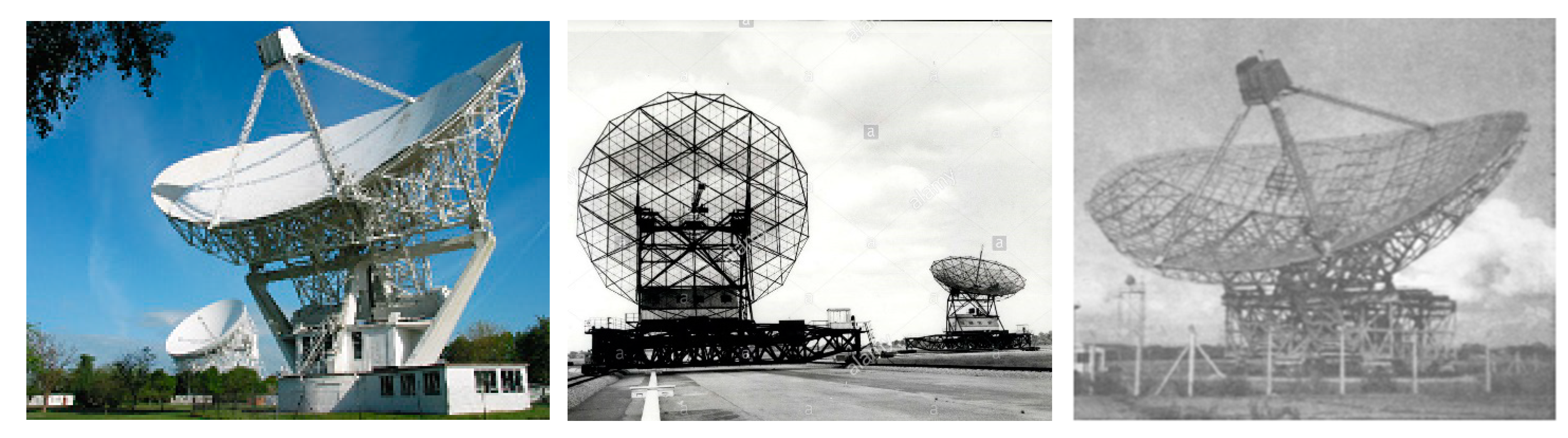
The second was Robin Conway’s smaller group that was developing new ways to measure the linear polarization of radio sources. This gives important information about their magnetic fields and their environment. In a pair of elegant papers in 1969, he and Philipp Kronberg laid out the principles of measuring polarization with a two-element interferometer [5,6]. However, their antennas (the Mk I and Mk II telescopes, see Figure 1) were only separated by 425 m so most radio sources, though polarized, were unresolved. On the other hand, the very long baselines used by Henry Palmer’s group resolved many of the sources but could not measure their polarization.

This seemed to me to be an irresistible challenge—to figure out how to combine the angular resolution of a radio-linked (and not phase stable) long baseline interferometer, with the methods developed by Conway and Kronberg to measure the linear polarization of the radiation.

So, I joined both groups though I was mostly supervised by Robin Conway, who had just returned from a sabbatical year at NRAO. We were assigned time with the 250 ft diameter Mk I telescope (needed because the polarized signals are weak) and the Mk III telescope, a light-weight version of the 125 × 85 ft Mk II with a mesh surface [7,8]. The Mk III telescope was located on the outskirts of the picturesque village of Wardle, Cheshire. (Really—Google it. It is near Nantwich). I should have recognized that as an omen because I have spent most of my working life trying to measure polarization with widely separated antennas. It was connected to Jodrell Bank by a radio link.

Only one paper was published from this experiment. It was on 3C 459, which had a clear result and served as proof of principle [9]. The set-up is described briefly in [9] and in my Ph.D. thesis (the 4th carbon copy, which has not aged gracefully these past 50 years). The Mk III telescope received only right hand circularly polarized radiation (RCP). The Mk I received both hands of circular polarization, and we switched between two ports of a square hybrid at one-minute intervals, receiving, alternately, left (L) and right (R) circular polarization, so the output of the correlator switched between RR* and LR* fringes. In the absence of instrumental effects (e.g., the leakage between left and right channels, defined in [5] and still known as “D terms”), RR* and LR* are proportional to the Stokes combinations I + V and Q–iU. We observed at 610 MHz.

The 24 km radio link had two channels: UHF (at 465 MHz) carrying the LO signal from Jodrell Bank to the Mk III, and a microwave link (at 7.5 GHz) returning the wide band astronomical signal back to Jodrell Bank and the correlator. Jodrell Bank and the Mk III had line of sight connectivity, but only barely. When a tall truck went over a bridge crossing the M6 motorway in Holmes Chapel, the link would be disrupted.

The radio link-maintained phase stability for several minutes, so we could reference the phase of the polarized fringe, ϕ_p, to that of the parallel hand fringe, ϕ_u. Even though we could not calibrate the absolute phase of either the parallel-hand fringe or the cross-hand fringe, the phase difference ϕ_p − ϕ_u was stable and depended only on sky quantities. This permitted long integrations of the polarized fringe, typically between 15 and 30 min.

With a single baseline, your u-v coverage is restricted to a single ellipse. If you have only observed the parallel hand fringes, the best you can do is fit a model to the fringe amplitude as a function of hour-angle and make a model of the unpolarized brightness distribution of the radio source. If you have also observed the cross-hand fringes you can do more. You can calculate the expected phase from your model, ϕ_u(model), at each point on the u-v ellipse. Then, you can estimate the phase of the cross-hand fringe alone as

ϕ_p(estimated) ≈ ϕ_p − ϕ_u + ϕ_u(model)

(1)

Then, with the cross-hand amplitudes and the estimated phases, you can now model the polarized brightness distribution of the radio source, including the distribution of the electric vector position angle (EVPA). Note that the polarized model is independent of the total intensity model. The leakage (D) term was estimated from observations of 3C147, which is essentially unpolarized at 610 MHz, and removed from the polarized fringe.

Although the atmosphere was stable enough at 610 MHz, the ionosphere most definitely was not. Faraday rotation could swing the EVPAs by several radians in daytime. The observed polarized fringe phases were corrected with estimates of the ionospheric Faraday rotation. These were calculated with an accuracy of about 10 degrees from hourly f₀F2 values from an ionosonde (which measures the maximum electron density in the ionospheric F2 layer) and an ionospheric model appropriate to the geomagnetic latitude of Jodrell Bank.

The radio source for which this whole setup worked particularly well was the aforementioned N type galaxy 3C 459 (z = 0.022), which had a simple structure. We modeled it [9] as a double radio source with a separation of 7.5 arcsec. The stronger component was coincident with the galaxy nucleus and was almost unpolarized. The weaker component was coincident with a faint optical luminosity visible on the Palomar red plate, and was strongly polarized at 8.8%. Including higher frequency data, the direction of the magnetic field appeared to be along the line separating the two components. Today, we would recognize this as a rather typical core-jet source in an AGN.

In 1974 they completed the LO loop and made the radio link phase stable. It became one of the six stations of the Multi Telescope Radio Linked Interferometer better known as MERLIN [10]. Because all the radio links were phase stable, MERLIN could measure polarization and carry out aperture synthesis, with sub-arcsecond resolution intermediate between that of the VLA and of intercontinental VLBI.

By 1996, the push to shorter wavelengths had made the Mk III telescope with its mesh surface no longer useful, and it was dismantled for scrap. Sic transit, etc.

3. The NRAO 3-Element Interferometer

At the end of 1969 I flew TWA (remember them?) to Washington DC, and drove down to Charlottesville, Virginia, to take up a postdoctoral fellowship at NRAO. As is common, the agreement was that I should spend half my time on projects connected to the Observatory, and half on whatever I chose. My project for the Observatory was to write software to calibrate the polarization (i.e., determine the D terms) of the 3-Element Interferometer located in Green Bank, WVa. I knew how to do that (once I had learned FORTRAN).

The 3-Element Interferometer consisted of three 85′ parabolic dishes, two of which could be moved to different stations up to a maximum baseline of 2700 m (Figure 2, left). It observed at frequencies of 2.7 GHz and 8.1 GHz simultaneously, and was built to gain experience in aperture synthesis for the proposed Very Large Array (VLA), which would be built over the next few years. There was also a fourth, moveable 45 ft antenna on a hilltop 35 km from Green Bank and connected by a radio link. That long baseline was used by Bruce Balick and Bob Brown to discover a very compact radio source at the center of our Galaxy in the direction of the constellation Sagittarius [11]. That, of course, is now known as the 4 million solar mass black hole called Sgr A* (pronounced saj-ay-star).

Each of the three antenna pairs operated as a two-element interferometer, but there were important differences compared to the interferometer I used at Jodrell Bank. (1) Each antenna received both hands of circular polarization without any switching, so four correlations were available on each baseline all the time. This allowed the u-v plane to be filled properly with the RL* and LR* fringes. (2) The same local oscillator signal was sent to each antenna, so both the parallel-hand and cross-hand fringes were stable, and their phases cold be calibrated by observing a source of known position. (3) The antennas had equatorial mounts, which meant that the dishes rotated with the sky. The D terms are a property of mainly the antenna feeds, and are fixed in the antenna frame. When the antenna rotates with the sky, it becomes difficult to separate the polarization due to the D terms from the polarization of the radio source. It is necessary to have a short list of unresolved calibration sources, whose polarizations are already known (from other short baseline or single dish measurements) and are thought to be (or hoped to be) non-variable. 3C 48, 3C 147 and 3C 286 were all used, and 3C 286 has become the default EVPA calibrator for the VLA and the VLBA. It is compact, strongly polarized, and unlike most compact sources, its EVPA has held remarkably steady for decades.

The above assumes that the calibrators are unresolved, or nearly so. For global VLBI at high frequencies this is almost never the case. This means that the D terms must be determined at the same time as determining the polarized structure of the calibration source. This is now implemented in the task LPCAL in the NRAO AIPS package [12].

The calibration software was written for the NRAO 3-element interferometer and put to good use. I do not know how many published images with linear polarization were produced by this instrument. A check with the SAO/NASA ADS does not reveal any. It was cumbersome to use because you had to wait for the antennas to be moved several times to do aperture synthesis. However, it was superb at measuring the properties of compact sources because it did not matter which configuration the antennas happened to be in. I used it with Philipp Kronberg to measure the linear polarization of a large number of extragalactic radio sources [13,14].

The appendix of [13] contains the derivation of, and a simple correction for the bias in measuring the amplitude of a vector signal in the presence of noise. It is barely original, but is cast in a form that radio astronomers find useful. The result is that [13] has received far more citations (614 and counting) than any other paper I have written.

I also initiated a program of monitoring at approximately two monthly intervals the flux and polarization at two wavelengths (11.1 and 3.8 cm) of all known or suspected variable extragalactic radio sources as of 1971. There had been extensive monitoring programs in total intensity, but monitoring the polarization was relatively rare. A notable exception has been the single dish program at the University of Michigan [15], et seq., whose long-term monitoring of the flux and polarization of a large number of quasars and AGN has been an important program in its own right and also an invaluable resource to the VLBI community (see Figure 2, right).

4. Brandeis University

In January 1972, I started at Brandeis University, which is in a suburb of Boston. I had just grown a beard so that I might look a bit older than my graduate students (the English system is very fast at both the undergraduate and the graduate levels). This was wise because it turned out that I was not. My first graduate student was Daniel Altschuler, who came from Uruguay. We continued the monitoring program with the Green Bank interferometer till 1975 and then published three papers [16,17,18]. In those days, the NRAO computer in Charlottesville was a mainframe IBM 360/50. It took punched cards for input, and our programs and all our data were in about 5 long boxes containing several thousand punched cards. I was always terrified of dropping a box on the floor and having to put all the cards back in correct order. Fortunately, that never happened.

Another feature of the IBM 360/50 will seem unimaginable to students today. Its “fast” random access memory (RAM) was a matrix of ferrite cores, exploiting magnetic hysteresis to store ones and zeros. Slower but much more back-up capacity was provided by magnetic disk stacks, and magnetic tape. The computer in Charlottesville had a total capacity of only 270 KB of RAM, but we could not even use all of that. During the day, it was divided into 3 partitions of 90 KB each, and most programs were expected to run with only 90 KB. At night you could request “large” partition and get 180 KB. This seems extraordinary when the smallest (solid state) flash drives today have storage capacities of Gigabytes. The Space Shuttle computers had ferrite core RAM. In the early 1980′s, when they needed some replacements, NASA discovered that nobody made them anymore.

The first of our three papers was on BL Lac objects, which at the time seemed very mysterious (were they quasars or galaxies or something else, and were their redshifts cosmological or something else?). In 1978 I attended the Pittsburgh Conference on BL Lac objects and talked about their radio properties [19]. When I started to talk about their polarization, I could see Margaret Burbidge sitting in the front row getting visibly agitated. After a while, she interrupted me and we sorted it out. On my slides showing tables and histograms of fractional polarization, I used Robin Conway’s notation of lower case m for fractional polarization. Of course, to an optical astronomer, m means something completely different.

In 1980, I was joined at Brandeis by David Roberts, who had just completed a postdoctoral fellowship at MIT in Bernie Burke’s group. They had been heavily involved in studying the gravitationally lensed “double quasar” 0957 + 561, with the VLA. On 18 May 1980, they tried to carry out a 600 MHz VLBI experiment observing the double quasar with an unusual mix of antennas: the Haystack 150′ (normally used for atmospheric research) together with the Green Bank 140′ antenna in the east, and the Owens Valley 130′ antenna in the west. While the east–east baselines showed steady fringes, the baselines to California showed huge phase and fringe rate fluctuations. When they realized they had been observing during the eruption of Mount St. Helens, it became clear that they were observing large scale travelling ionospheric disturbances (TIDs) triggered by the volcano [20,21]. Such large disturbances had not been seen since the days of nuclear testing in Nevada.

Dave Roberts had also worked extensively on Quasat, and other space VLBI projects [22], and knew a lot about VLBI. I knew something about measuring polarization with interferometers, so we decided to put these together and attempt polarization observations at VLBI resolution.

The first successful attempt to do this actually predated our first observations by several years. This was the observations of the 1665 MHz OH masers in the star-forming region W3(OH) [23]. The observations were made in 1978 using 6 antennas (Fort Davis, Green Bank 140′, Haystack, Owens Valley, Vermillion River, Dwingeloo). The data were collected using the Mk II recording system. All antennas had both left and right polarized feeds, and they switched between left and right at 1 s intervals (in synchrony to get Stokes V, and then with some antennas out of phase to get cross polarized fringes for Stokes Q and U). OH masers can be strongly circularly polarized as well as linearly polarized, at levels of several tens of percent. This means that the correction for the leakage D terms was relatively unimportant, and they decided to neglect it altogether. The complexity of the experiment was such that it was not actually published till 1988. With the VLBA, spectral line polarization VLBI observations have become much more feasible, and a good description of the data reduction techniques can be found in [24].

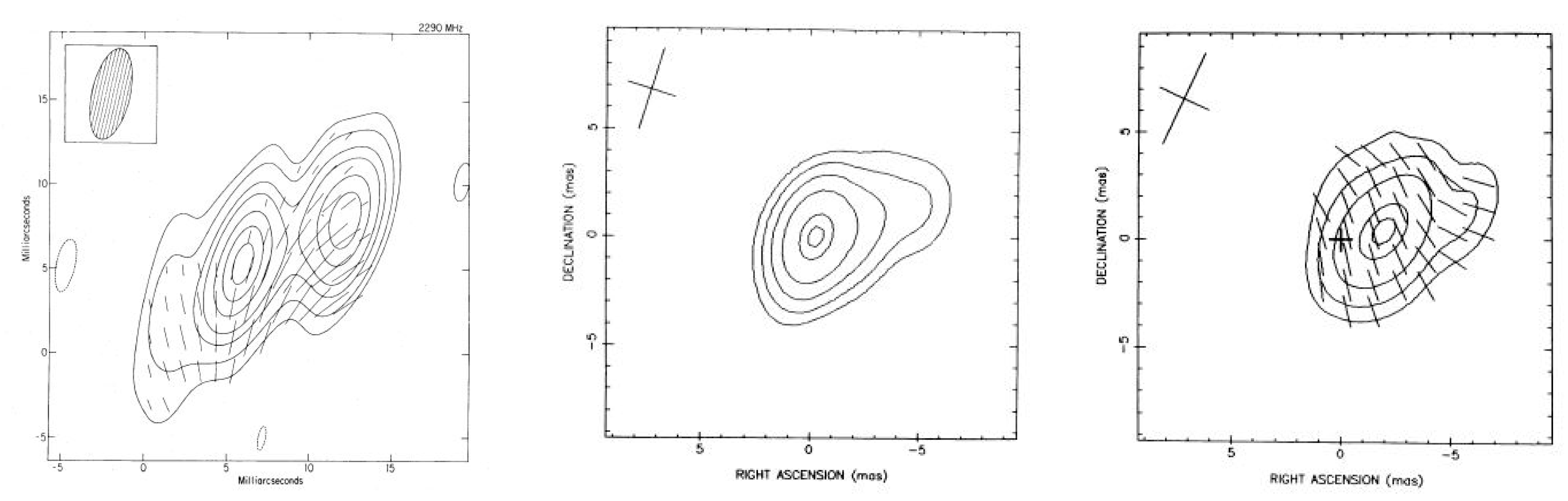
The first continuum VLBI polarization image was published in 1984 by Cotton et al. [25] (see Figure 3). The image was of the quasar 3C 454.3 at a wavelength of 13 cm. The observations were made in 1980, also using the Mk II recording system with its rather limited bandwidth of 2 MHz. Their array included the NASA Deep Space Network (DSN) antennas at Goldstone and Madrid, together with Haystack, NRAO (140′), Ft. Davis and Onsala. The Goldstone and Madrid DSN antennas were equipped with dual polarization feeds; the others had only right circularly polarized feeds. This had two consequences: the coverage of the u-v plane in polarization was limited to those baselines that included a DSN antenna, and also that the coverage was asymmetric with respect to conjugate u-v points. Asymmetric coverage of the u-v plane necessarily causes the ‘dirty beam’ to be complex, requiring a complex CLEAN. Their image of the polarized radio emission is shown in Figure 3 (left). Bill Cotton was very busy with a wide range of different projects, and I am not sure if his group ever published another VLBI polarization image, though he did publish some very useful papers on how to do it (e.g., [26]).

In 1977, the Mk III recording system became available for VLBI. It could record 28 tracks, each of 2 MHz, for a total bandwidth of up to 56 MHz. This represented a huge increase in sensitivity, which was just what was needed for measuring polarization. Additionally, we realized that the problems of measuring polarization with VLBI and independent local oscillators, was little different in principle from what I did for my Ph.D. thesis with a radio linked interferometer. Recognizing this, Dave Roberts and I started submitting observing proposals soon after he arrived at Brandeis. Our first few observing proposals were not successful. One proposal referee remarked rather sourly that we appeared to have a secret but would not say what it was. We learned that several other astronomers had received observing time for similar projects, but had not been able to produce results. I suspect that one of the reasons for this is that they tried to use AIPS, designed for the VLA, with all dual polarization receivers and identical antenna mounts, and certainly not designed (at that time) for polarization sensitive VLBI.

In 1981 we got some observing time with the Mk III system. We used 4 antennas: the 120′ antenna at Haystack, the Greenbank 140′, the VLA, where all 27 antennas were phased up to act as a single antenna of equivalent diameter 130 m, and the Owens Valley 130′. Green Bank and the VLA had both left- and right-hand polarized feeds, while Haystack and Owens Valley received only left-hand circular polarization. Three of the antennas had alt-azimuth mounts, but the Green Bank 140′ had an equatorial mount (its 17.5 ft diameter bearing on the polar axis was, at the time, the biggest ball bearing in the world). The experiment was successful (see Figure 3, center and right). One reason was that I did not try and force AIPS to do a job it was not designed for. Instead, I wrote all the calibration and imaging software ab initio (in FORTRAN) so that it did exactly what we wanted it to do, including all the diagnostics we needed, and we understood every line of the code.

The Mk III tapes were correlated at Haystack Observatory, which is only 52 km from Brandeis. It was very useful to be there to help coordinate the changes in procedure needed to recover the cross-hand fringes. Even though there were atomic clocks at each antenna to generate the local oscillator signals and to write time markers on the tapes, it was still necessary to search in both delay and delay rate to find the sweet spot for the parallel-hand fringe detections. From the size of the search area, the rule of thumb was that apparent detections with signal to noise ratios < 7 were not reliable. Cross-hand fringes are generally weaker than parallel hand fringes by a factor of 10–100, and almost never reach that threshold. The strongest and most strongly polarized sources such as 3C345 and 3C279 could meet the SNR > 7 criterion for the cross-hand fringes, but the majority of the sources we observed could not. However, because the parallel hands already told us where to look in delay-delay rate space, the SNR > 7 criterion did not apply. We could use (and integrate) cross-hand fringes of arbitrarily small SNR. This referencing of cross-hand fringes to the parallel hands is closely related to what was done with the Mk I–Mk III radio linked interferometer—see Equation (1). There is one extra component of delay that the parallel hands cannot determine. This is the station-based delay offsets between the right- and left-hand signal paths. These are typically a few to a few tens of nanoseconds in the multiband delay at each antenna, and manifest themselves as a rotation of the measured EVPA. A single observation of a strongly polarized calibration source of known EVPA (invariably 3C 286) is sufficient to determine all the delay offsets. This is all explained with great clarity in Leslie Brown’s Ph.D. dissertation and in [28].

There were some features of the imaging and CLEAN routines that may be of interest. With only 4 or 5 antennas, the u-v coverage is extremely sparse. It seemed unnecessary and maybe even detrimental to convolve the u-v data onto a square grid. That meant that we could not use the Fast Fourier Transform to make the dirty image and dirty beam. However, it did not matter because with so few data, the difference in speed between the direct Fourier Transform and the Fast Fourier Transform was not very important, and we avoided introducing any errors from the convolution process. (To be clear, we calculated Fourier components using the actual u, v values, and added their contributions on a grided image plane. We calculated the dirty beam the same way).

The CLEAN algorithm was different too. In some imaging software, both the RL* and LR* correlations are required to be present. If one is absent, the other is flagged and not used. The VLA, with 351 baselines, can afford to be profligate with its data; we could not. In the early experiments some antennas were equipped with only one hand of polarization and would have been flagged out entirely (this was also true of the spectral line VLBI experiment [23], and of Cotton’s observations of 3C 454.3 [25]). If you do not have the conjugate data point to a cross-hand correlation, then the coverage of the u-v plane is asymmetric, and the dirty beam is complex. This then requires a complex CLEAN. There is no difficulty with this either conceptually or in practical execution, and you are maximizing the use of your observations.

Graduate students played a huge role in developing the software, making the observations and analyzing the data at this exciting time. We had a long line of outstanding graduate students at Brandeis. The ones who helped us develop VLBI polarimetry included Scott Aaron, Joanne Attridge, Leslie Brown, Tingdong Chen, Teddy Cheung, Wesley Cobb, Denise Gabuzda, Mark Holdaway, Dan Homan, Ron Kollgaard, George Mollenbrock, Roopesh Ojha, Bob Potash, and postdoctoral fellow Tim Cawthorne from Cambridge. Together, we published about 30 papers in refereed journals, and a similar number in conference proceedings.

Mark Holdaway’s main project was a study of using polarized entropy for making images. This had not been done with real data before. It built on definitions of the entropy of polarized radiation proposed by John Ponsonby at Jodrell Bank [29]. Mark developed software to make polarized images using maximum entropy methods (MEM). We wrote a short paper for an IEEE meeting [30], but the bulk of his work is in his Ph.D. dissertation, available on ADS [31]. MEM tends to be computationally expensive, and the images depend on the assumed priors. It did not gain much traction until recently, when it was incorporated into some of the imaging approaches used for the Event Horizon Telescope [32,33]. Denise Gabuzda’s group has also developed the use of maximum entropy methods for VLBI polarization imaging [34].

5. The Very Long Baseline Array (VLBA)

This array of ten identical 25 m antennas (all on USA territory—that was a design requirement) was proposed to the NSF in 1982, and by 1994 all ten antennas had been built were open for business. It was always intended that the VLBA would be able to make images in linear polarization, so every antenna had dual polarization feeds at every wavelength. What was needed was the calibration software to determine the D terms at each antenna, and this was written by Kari Leppanen, a graduate student from the Helsinki University of Technology in Finland [12].

The VLBA was and is a superb instrument—a far cry from the early days of Mk III VLBI, with its ragamuffin collection of antennas only some of which had dual polarization feeds. Since the antennas in the Mk III network all belonged to different observatories, it was necessary to negotiate with each one to borrow their antenna for a few days a year (it had to be the same few days, of course) so that VLBI experiments could be carried out. The VLBA was like a breath of fresh air. The whole array was available all the time, and you could do VLBI 24/7. This of course resulted in a huge increase in the number of papers published based on VLBI observations and greatly expanded the scientific questions you could ask.

The uniformity of the antennas and the stability of the electronics permitted greater precision in the calibration of the data. The great increase in availability of observing time encouraged monitoring programs that imaged both linear polarization and total intensity. The Brandeis group did this for a few years [35,36], but the programs that persist to this day are the Boston University group, that has pushed to shorter wavelengths and includes monitoring optical polarization (e.g., [37,38]), and the MOJAVE project that was originally a 15 GHz total intensity monitoring program to study jet kinematics. It extended its goals to include polarization when Matt Lister and Dan Homan were both Jansky fellows at NRAO. They now have more than 20 years coverage on over 400 sources, mostly at 15 GHz, and have published over 100 papers [39,40].

With the repeated observations of many sources at a fast enough cadence, it became clear that the best way to show the evolution in time of the structure and polarization is to make movies. I think Teddy Cheung was the first to do this for his undergraduate senior thesis at Brandeis, later written up as an NRAO memo and posted on astro-ph [41]. His movies were on our website for many years. Today the MOJAVE website [42] is a treasure trove of such movies, and one can happily spend hours watching and trying to interpret how the flux and polarization of your favorite sources evolve.

6. Polarization Sensitive Observations from Space with VSOP/HALCA and RadioAstron

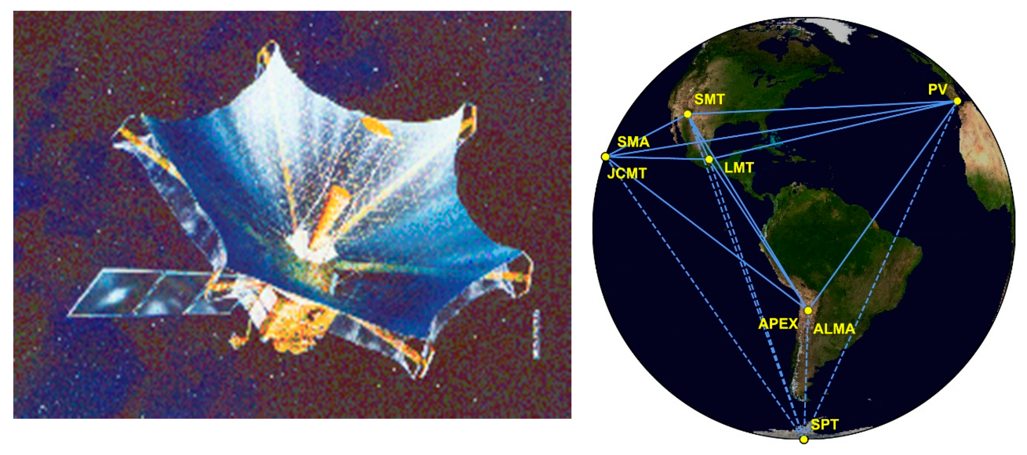
In 1997, Japan launched an 8 m antenna in a highly elongated orbit, dedicated to VLBI. It observed at 1.6 and 5 GHz in conjunction with ground-based antennas including the VLBA until 2005. The antenna had a very unusual design (see Figure 5, left). It rode into space furled like an umbrella, and was unfurled once it was in zero-g orbital flight. This must have been a heart-stopping moment for the engineers on the ground because they had never been able to test it on the ground in Earth’s strong gravity.

At apogee, its altitude was about 21,000 km, giving baselines to the VLBA antennas about 3 times longer than what was normally available, and its highly elliptical orbit sampled a wide swath of spacings in the u-v plane. It had a single polarization (LCP) feed enabling limited imaging in linear polarization. For such an unusual antenna, the D terms were quite small–about 3% at 1.6 GHz and about 9% at 5 GHz. This is described in [43] together with some of the special problems of calibrating a space antenna.

Operations were ended at the end of 2005 by which point it had far exceeded its expected 3-year lifespan. Denise Gabuzda wrote a valedictory article [44] describing the contributions (about 40 papers) VSOP had made to the understanding of magnetic fields in jets.

RadioAstron was a Russian 10 m dish launched in 2011 into a highly elongated orbit that reached an apogee height of 350,000 km (comparable to the distance of the Moon). It had both RCP and LCP feeds and at 22 GHz had a resolution of about 21 micro-arcseconds (but a synthesized beam at least as elliptical as its orbit). Its primary mission was measuring the brightness temperatures of the most compact radio cores. The first 22 GHz polarization sensitive observations were of BL Lac [45]. In 2019, communications from the ground to the spacecraft were lost, but it too had lasted much longer than its expected lifespan.

7. Circular Polarization at Milliarcsecond Resolution

The outstanding performance of the VLBA led directly to the detection of Circularly Polarized radiation (CP) at milliarcsecond resolution [46]. The single dish or short baseline interferometer measurements of the polarization of extragalactic sources had shown that the fractional CP is usually only a few tenths of a percent, and almost never more than 1%. (As in the case of linear polarization observations with VLBI, the first examples of circular polarization observations with VLBI came from spectral line observers looking at molecular masers in star-forming regions (e.g., [47]). These can exhibit fractional CP at the level of several tens of percent, and special techniques are not required).

I thought of VLBI CP observations of extragalactic continuum sources as the next observational challenge (and therefore irresistible to attempt). The major complication was that the feeds of the VLBA were all dual polarized right- and left-hand circular polarization (RCP and LCP). In the language of Stokes parameters [5,48], the cross-hand correlations are RL* ∝ Q + iU and LR* ∝ Q − iU. The total intensity, I, only enters through the D terms, which are usually small, so this is a good way to measure linear polarization. However, the parallel hand correlations are RR* ∝ I + V and LL* ∝ I − V. The tiny V signal is riding on top of the large total intensity signal. In general, subtracting two large signals to detect a small difference is a bad idea, because you end up detecting the errors in the amplitude calibration of the two parallel hand correlations.

Some arrays have linearly polarized feeds, often crossed dipoles, such as ATCA [49] and ALMA [50]. Then, if the channels are X and Y, then for an interferometer XX* ∝ I + Q and YY* ∝ I − Q, which is a bad way to measure Q, but XY* ∝ U + iV and YX* ∝ U − iV, which is a good way to measure V (see [5,48] for the full set of correlations). This is a bit counter intuitive–that you would prefer circularly polarized feeds for measuring linear polarization, and linearly polarized feeds for measuring circular polarization. The result of all this is that ATCA, which has linearly polarized feeds, can detect fractional CP at levels down to an astonishing 0.03% [49], while the VLBA, with circularly polarized feeds, is about a factor of 10 less sensitive (e.g., [51]).

I did not believe that the VLBA could calibrate the fringe amplitudes to the required accuracy of a few tenths of a percent, so I tried to think of other ways of doing it. (I was greatly encouraged by simulated images of parsec scale jets in circular polarization by Tom Jones [52]).

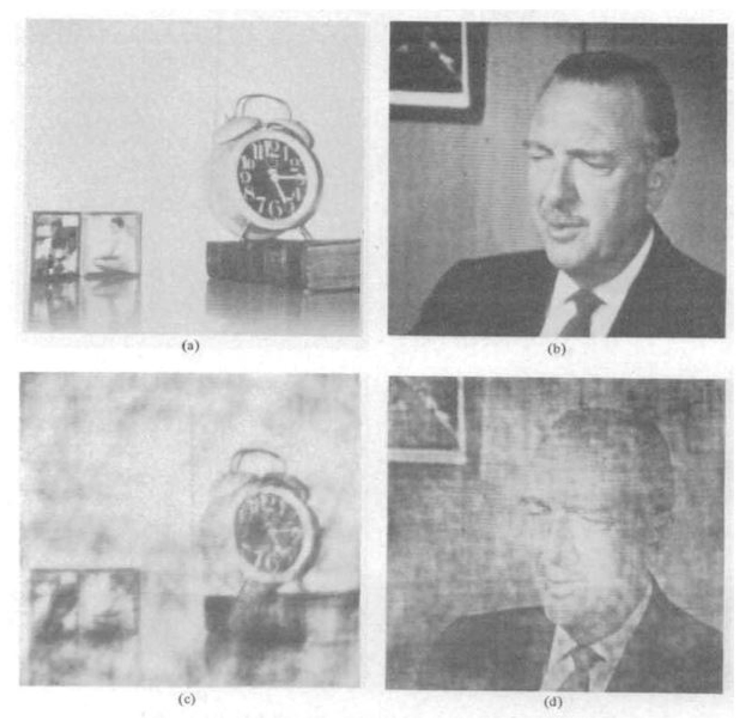
My first thought was to dispense with the amplitude information altogether, and see if we could extract information about V from the phases alone. This was suggested by a remarkable paper about imaging that I happened across [53]—see Figure 4.

For our purposes, we could set the fringe visibility amplitudes equal to unity but keep the phases as measured. This will obviously not work if the source is an unresolved point with circular polarization, because all the phases are zero. If the CP is not sitting on the core, then we obtain an anti-symmetric image of Stokes V. If this seems strange, I would point out that the RR* (∝I + V) and LL* (∝I − V) closure phases will differ if there is a true V signal present. Furthermore, whatever you do to the amplitudes will not remove the V signal from the phases.

Working with Dan Homan, we devised two more ways of mitigating the amplitude calibration problem with VLBA observations. All three approaches are described in [54], and examples given. The second, “zero V self-cal” exploits the fact that the gains we are trying to determine multiply the visibilities while the V signal is additive. Incorrect gains (such as setting all the amplitudes of the RR* and LL* fringes equal to each other) cannot destroy a real V signal, but merely redistributes it in the image. The third method, “transfer of gains,” works best if you have observed many sources. It assumes that all sources can potentially be used as unpolarized (zero V) gain calibrators (which is mostly true, but you do not know which ones because nearly all of your target sources are variable), until the sources with real V stick out and are removed from the calibration procedure.

We first applied the transfer of gains method to 3C 279, which was part of our 12-blazar monitoring program [35]. This led to the first published result of a measurement of CP at milliarcsecond resolution [46]. A more extensive application and testing of the transfer of gains method was on 40 sources that Joanne Attridge had previously observed for a linear polarization survey [55]. The experiment was very successful, detecting 11 sources that exhibited CP at the 3σ level or higher, and nearly quadrupling the number of sources with CP detections at milliarcsecond resolution at that time. This approach is tailor-made for programs such as MOJAVE [51] or other surveys which look at a large number of sources [56].

Clearly my original guess that it would not be possible to calibrate the RR* and LL* fringes with sufficient accuracy to measure CP was wrong. That you can measure CP rather straightforwardly (if you are very careful and have lots of potential calibrators) is a tribute to the remarkable stability of the electronics of the VLBA.

8. Rotation Measures and Rotation Measure Gradients

The VLBA is agile at switching between observing frequencies. This allows one to map the distribution of Faraday rotation in jets and cores, but there are some practical difficulties that must be paid attention to.

One is that the resolution changes as one changes frequency. It is not enough to convolve the images down to the resolution of the lowest frequency, because the u-v coverages are still different. MOJAVE [57] mitigated this by flagging the shortest baselines at the lowest frequency and flagging the longest baselines at the highest frequency, but they are discarding information.

Another is the registration of the images. The apparent core in an image is located near the τ = 1 surface [58]. You cannot align the images on the core because it moves closer to the jet apex with increasing frequency (“the core shift” [59]). Instead, you should align on a bright optically thin feature farther downstream, or if the jet is rather smooth, cross-correlate the optically thin emission.

For sources where the jet is sufficiently resolved, you can measure the rotation measure gradient across the jet. This been somewhat contentious, with arguments about how well resolved the jet must be to determine a reliable gradient. The MOJAVE program [57] used a sample of 149 sources, and found only 4 sources with unequivocal transverse gradients by their requirements (jet width > 1.5 beamwidths). The number of claimed RM gradients is much higher than this [60], et seq., which also contains a good discussion of the dispute. Gabuzda (personal communication) has now claimed to have measured reliable transverse RM gradients in more than 50 sources.

Transverse RM gradients are very interesting because a natural explanation for the gradient is that the magnetic field in the jet (and surrounding the jet) has a toroidal component, which is superposed on a larger scale foreground rotation measure (e.g., [61]). By Ampère’s law, a toroidal magnetic field requires that a current flows down the jet. The current therefore generates both part of the field (in conjunction with the poloidal component) that gives rise to synchrotron radiation from the jet, and also the magnetic field in the plasma surrounding the jet that gives rise to the RM gradient. Jet currents are an inevitable consequence of toroidal magnetic fields. Inserting typical values for the magnetic field and jet radius, we expect currents of the order 10¹⁷–10¹⁸ A [62].

Rotation Measure mapping together with observations of linear and circular polarization offer a wealth of physical information that is unavailable from total intensity observations alone. This is what makes them so alluring. Indeed, Gabuzda and others have written interesting papers that try to connect RM gradients and circular polarization to the spin of the central black hole [63,64].

9. The Event Horizon Telescope

Operating at 230 GHz and spanning almost an Earth diameter, the EHT has a resolution of about 20 micro-arcseconds. The high observing frequency together with the small number of antennas (especially in 2017) has presented special challenges to the calibration and imaging of the data, both in total intensity and in polarization [65,66,67].

At 230 GHz, the array is very much at the mercy of the weather. Even though the antenna sites are among the highest and driest places on Earth, phase fluctuations due to tropospheric water vapor turbulence limit integration times typically to a few seconds.

Eight observatories at six geographic locations participated in the 2017 observations (see Figure 5), but some clarification is needed. The South Pole Telescope can see Sgr A*, but not M87, which is above the equator. APEX and ALMA are only 2 km apart. That is actually very useful for calibration, but for imaging, they effectively count as one site. The (typically) 37 or so 12 m antennas of ALMA that were phased up to act as a single antenna of equivalent diameter 70 m all had crossed dipoles for feeds. These were converted to RCP and LCP in the subsequent software [50]. Similarly, the SMA (submillimeter array) and the JCMT (James Clerk Maxwell Telescope) are about 150 m apart on the top of Mauna Kea, and also count as one site for imaging purposes. The SMA was dual polarization, but the JCMT was single polarization. For the first 3 days of the 2017 campaign, it received RCP and for the last 3 days it received LCP. As in the case of the ALMA-APEX, the short baseline was very useful for calibration purposes. The rest of the antennas of the EHT had dual (RCP and LCP) polarization receivers. The details of the array, its calibration and the imaging methods used can be found in [66,67,68].

In effect, the 2017 observations of M87 were made with a 5-station array. This is reminiscent of our earliest days with the Mk III system.

With only 5 antennas, imaging in either total intensity or linear polarization is challenging. With the EHT, new approaches have been developed, and these are interesting and welcome. Since the early days of aperture synthesis, the usual way to make an image was to take the u-v data in the u-v plane, and Fourier transform it into an image in the x-y plane, and then deconvolve the image using the CLEAN algorithm [69]. There may also be several rounds of self-calibration. This approach is often referred to as “inverse modeling.” This is the standard way of making images for the VLA or for the VLBA and is performed by the program DIFMAP [70].

Two new and rather similar versions of “forward modeling” are described in [71]: eht-imaging [32,72] and SMILI [33,73]. In forward modeling you are trying to find an image that fits the visibilities (fringe amplitudes and closure phases) subject to other constraints called regularizers that encourage desirable image properties. The latter might include an entropy term which enforces positivity, and TV “total variation” which encourages pixel to pixel smoothness and image compactness. For more details see Appendix A of [71]. The imaging was carried out by independent teams using each of these methods. In the end, they averaged all three images on the day with the best data to produce the iconic image that was shown to the world on 10 April 2019.

For the linear polarization data, there are additional problems in figuring out the D terms of the EHT antennas [68]. What you need is one or two sources that are unresolved or unpolarized [74]. At 20 micro-arcsec resolution we do not know of any. It therefore becomes necessary to solve for the polarized structure of the calibrator source at the same time as determining the D terms. Cotton briefly discusses this in [26], and Leppanen incorporates it into his calibration program [12] now incorporated into AIPS as the task LPCAL. To do it with only a five station array is not easy. Ironically, it turns out that one of the best calibrators is M87* itself, because its structure is simple, and it is not very strongly polarized. Much more information on all of this, especially regarding the extensive consistency checks and imaging parameter surveys that were carried out can be found in [68].

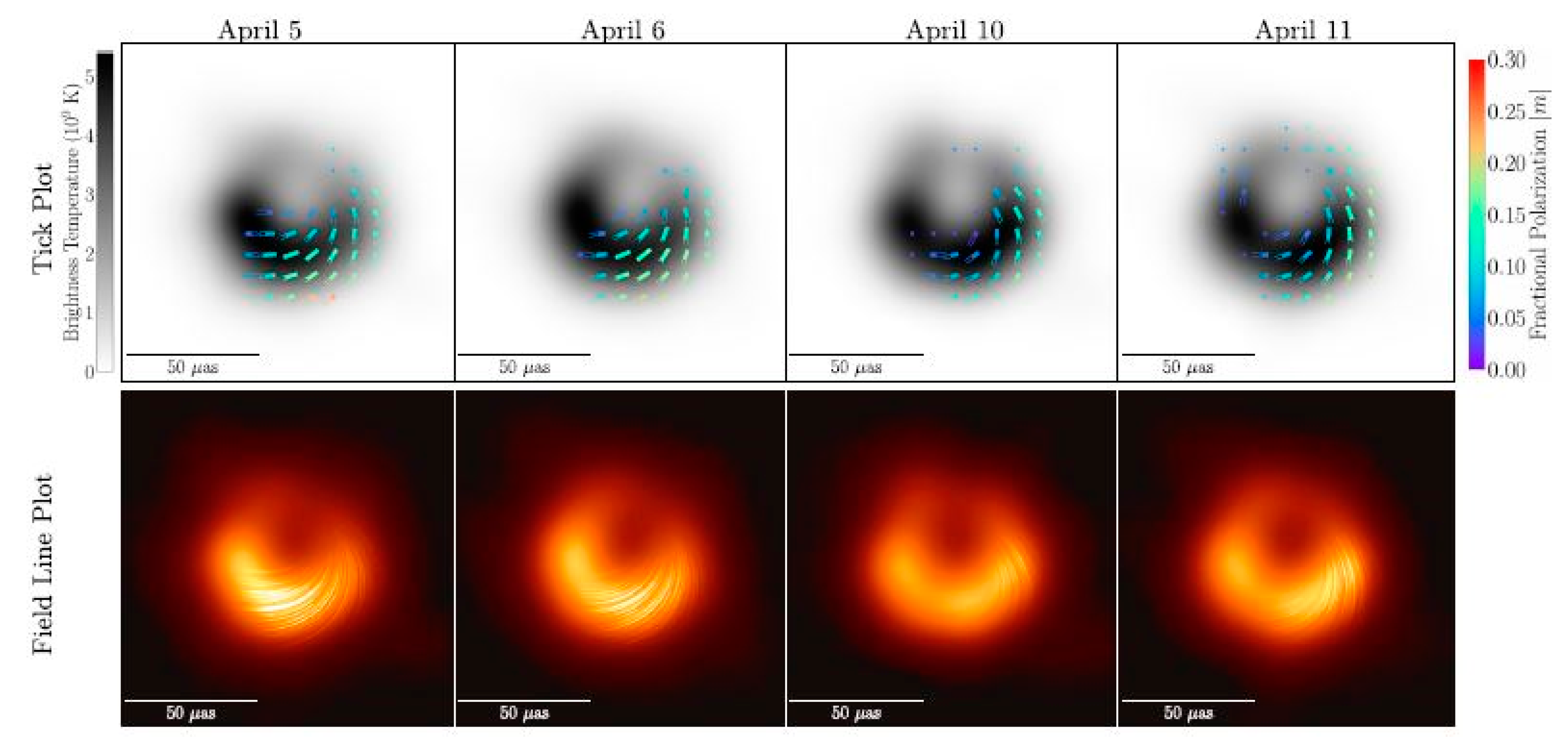
In the end, five different imaging approaches were used to determine D terms and make images of M87* in linear polarizations (see Figure 6). Again, details can be found in [68].

The publication of the polarization image of M87* is an important milestone in the story of the development of polarization VLBI, but the story never ends. In 2017 the EHT also observed Sgr A*, which we know exhibits both linear and circular polarization [76], but varies on a timescale of minutes. Now that is an imaging challenge! There are new observations and new antennas have been added to the array. Additionally, perhaps we will get an antenna in space again.

The author thanks Jim Moran, Ralph Spencer and Denise Gabuzda for helpful conversations, and to the referees all of whom substantially improved the clarity of the paper. The author is solely responsible for all errors of fact and memory, and would greatly appreciate additional errors being pointed out to him. This paper loosely emulates Ralph Spencer’s paper titled “An Old Fogey’s History of Radio Jets” at the jet meeting held in Crete in 2017 [77]. We need more “old fogey” or “senior recollection” or “unauthorized accounts.” They tell the back stories of how science is done and how it progresses, and these rarely makes it into print. However, I believe them to be of interest and value to our colleagues in similar but parallel fields, and especially to graduate students entering the field. How else will they learn this background information? I, therefore, urge all colleagues who have a story to tell to put pen to paper and share it with the community and future students.

References

- Elgaroy, O.; Morris, D.; Rowson, B. A Radio Interferometer for Use with Very Long Baselines. Mon. Not. R. Astron. Soc. 1962, 124, 395–403. [Google Scholar] [CrossRef] [Green Version]
- Palmer, H.P.; Rowson, B.; Anderson, B.; Donaldson, W.; Miley, G.K. Radio Diameter Measurements with Interferometer Baselines of One Million and Two Million Wavelengths. Nature 1967, 213, 789–790. [Google Scholar] [CrossRef]
- Donaldson, W.; Miley, G.K.; Palmer, H.P.; Smith, H. Interferometric Observations with a Baseline of 127 Kilometers—I. Mon. Not. R. Astron. Soc. 1969, 146, 213–219. [Google Scholar] [CrossRef] [Green Version]
- Donaldson, W.; Miley, G.K.; Palmer, H.P. Interferometric Observations with a Baseline of 127 Kilometers—II. Mon. Not. R. Astron. Soc. 1971, 152, 145–158. [Google Scholar] [CrossRef] [Green Version]
- Conway, R.G.; Kronberg, P.P. Interferometric Measurement of Polarization Distributions in Radio Sources. Mon. Not. R. Astron. Soc. 1969, 142, 11–32. [Google Scholar] [CrossRef] [Green Version]
- Kronberg, P.P.; Conway, R.G. Measurements of the Integrated Linear Polarization of Discrete Radio Sources. Mon. Not. R. Astron. Soc. 1970, 147, 149–160. [Google Scholar] [CrossRef]
- Palmer, H.P.; Rowson, B. The Jodrell Bank Mark Ill Radio Telescope. Nature 1968, 217, 21–22. [Google Scholar] [CrossRef]
- Critchley, J.; Palmer, H.P.; Rowson, B. Observations of Radio Sources with an interferometer of 24-km Baseline-1. Mon. Not. R. Astron. Soc. 1972, 160, 271–282. [Google Scholar] [CrossRef] [Green Version]
- Wardle, J.F.C. The Structure and Polarization of 3C 459 at 610 MHz. Astrophys. Lett. 1971, 8, 53–55. [Google Scholar]
- Davies, J.; Anderson, B.; Morison, I. The Jodrell Bank radio-linked interferometer network. Nature 1980, 288, 64–66. [Google Scholar] [CrossRef]
- Balick, B.; Brown, R.L. Intense sub-arcsecond structure in the Galactic center. Astrophys. J. 1974, 194, 265–271. [Google Scholar] [CrossRef]
- Leppanen, K.J.; Zensus, J.A.; Diamond, P.J. Linear Polarization Imaging with Very Long Baseline Interferometry at High Frequencies. Astron. J. 1995, 110, 2479–2492. [Google Scholar] [CrossRef]
- Wardle, J.F.C.; Kronberg, P.P. Linear Polarization Measurements of Extragalactic Radio Sources at 3.71 and 11.1 cm. Astrophys. J. 1974, 194, 249–255. [Google Scholar] [CrossRef]
- Kronberg, P.P.; Wardle, J.F.C. Further Linear Polarization Measurements of Extragalactic Radio Sources at 3.71 and 11.1 cm. Astron. J. 1977, 82, 688–691. [Google Scholar] [CrossRef]
- Aller, H.D.; Olsen, E.T.; Aller, M.F. Linear Polarization and Flux Density Variations in the Radio Galaxy 3C 120. Astron. J. 1976, 81, 738–742. [Google Scholar] [CrossRef]
- Altschuler, D.R.; Wardle, J.F.C. Radio Properties of BL Lac type Objects. Nature 1975, 255, 306–310. [Google Scholar] [CrossRef]
- Altschuler, D.R.; Wardle, J.F.C. Observations of the Flux Density and Linear Polarization of Compact Extragalactic Radio Sources at 3.7 and 11.1 cm Wavelength. Mem. R. Astron. Soc. 1976, 82, 1–67. [Google Scholar] [CrossRef] [Green Version]
- Altschuler, D.R.; Wardle, J.F.C. Observations of the Flux Density and Linear Polarization of Compact Extragalactic Radio Sources at 3.7 and 11.1 cm Wavelength—II. Mon. Not. R. Astron. Soc. 1977, 179, 153–178. [Google Scholar] [CrossRef] [Green Version]
- Wardle, J.F.C. A Survey of Radio Polarization and Variability. In Proceedings of the Pittsburgh Conference on BL Lac Objects, Pittsburgh, PA, USA, 24–26 April 1978; pp. 39–50; Discussion 50–52. [Google Scholar]
- Roberts, D.H.; Allen, B.R.; Bennett, C.L.; Burke, B.F.; Clark, T.A. Detection of the 18 May 1980, Explosion of Mt. St. Helens by Very Long Baseline Interferometry. Bull. Am. Astron. Soc. 1980, 12, 814. [Google Scholar]
- Roberts, D.H.; Rogers, A.E.E.; Allen, B.R.; Bennett, C.L.; Burke, B.F.; Greenfield, P.E.; Lawrence, C.R.; Clark, T.A. Radio Interferometric Detection of a Travelling Ionospheric Disturbance Excited by the Explosion of Mount St. Helens. J. Geophys. Res. Space Phys. 1982, 87, 6302–6306. [Google Scholar] [CrossRef]
- Roberts, D.H.; Morgan, S.H.; Burke, B.F.; Jordan, J.F.; Preston, R.A.; Hamilton, E.C. Radio Interferometry from Space Platforms. Proc. SPIE Opt. Platf. 1984, 493, 120–132. [Google Scholar]
- Garcia-Barreto, J.A.; Burke, B.F.; Reid, M.J.; Moran, J.M.; Haschick, A.D.; Schilizzi, R.T. Magnetic Field Structure of the Star-forming Region W3(OH): VLBI Spectral Line Results. Astrophys. J. 1988, 326, 954–966. [Google Scholar] [CrossRef]
- Kemball, A.J.; Diamond, P.J.; Cotton, W.D. Data Reduction Techniques for Spectral Line VLBI Observations. Astron. Astrophys. Suppl. Ser. 1995, 110, 383–394. [Google Scholar]
- Cotton, W.D.; Geldzahler, B.J.; Markaide, J.M.; Shapiro, I.I.; Sanroma, M.; Rius, A. VLBI Observations of the Polarized Radio Emission from the Quasar 3C 454.3. Astrophys. J. 1984, 286, 503–508. [Google Scholar] [CrossRef]
- Cotton, W.D. Calibration and Imaging of Polarization Sensitive Very Long Baseline Interferometer Observations. Astron. J. 1993, 106, 1241–1248. [Google Scholar] [CrossRef]
- Roberts, D.H.; Wardle, J.F.C. Polarization Distributions in Compact Radio Sources. In Symposium -International Astronomical Union; Swarup, G., Kapahi, V.K., Eds.; Cambridge University Press: Cambridge, UK, 1986; Volume 119, pp. 141–147. [Google Scholar]
- Brown, L.F.; Roberts, D.H.; Wardle, J.F.C. Global Fringe Fitting for Polarization Sensitive VLBI. Astron. J. 1989, 97, 1522–1532. [Google Scholar] [CrossRef]
- Ponsonby, J.E.B. An entropy measure for partially polarized radiation and its application to estimating radio sky polarization distributions from incomplete aperture synthesis data by the maximum entropy method. Mon. Not. R. Astron. Soc. 1973, 163, 369–380. [Google Scholar] [CrossRef] [Green Version]
- Holdaway, M.A.; Wardle, J.F.C. Maximum entropy imaging of polarization in very long baseline interferometry. Proc. SPIE 1990, 1351, 714–724. [Google Scholar]
- Holdaway, M.A. Maximum Entropy Imaging of Radio Astrophysical Data. Ph.D. Thesis, Brandeis University, Waltham, MA, USA, 1990. [Google Scholar]
- Chael, A.A.; Johnson, M.D.; Narayan, R.; Doeleman, S.S.; Wardle, J.F.; Bouman, K.L. High-resolution Linear Polarimetric Imaging for the Event Horizon Telescope. Astrophys. J. 2016, 829, 11–26. [Google Scholar] [CrossRef]
- Akiyama, K.; Ikeda, S.; Pleau, M.; Fish, V.L.; Tazaki, F.; Kuramochi, K.; Broderick, A.E.; Dexter, J.; Mościbrodzka, M.; Gowanlock, M.; et al. Superresolution Full-polarimetric Imaging for Radio Interferometry with Sparse Modeling. Astron. J. 2017, 153, 159–171. [Google Scholar] [CrossRef] [Green Version]
- Coughlan, C.P.; Gabuzda, D.C. High resolution VLBI polarization imaging of AGN with the maximum entropy method. Mon. Not. R. Astron. Soc. 2016, 463, 1980–2001. [Google Scholar] [CrossRef] [Green Version]
- Homan, D.C.; Ojha, R.; Wardle, J.F.C.; Roberts, D.H.; Aller, M.F.; Aller, H.D.; Hughes, P.A. Parsec-Scale Blazar Monitoring: Flux and Polarization Variability. Astrophys. J. 2002, 568, 99–234. [Google Scholar] [CrossRef]
- Homan, D.C.; Ojha, R.; Wardle, J.F.C.; Roberts, D.H.; Aller, M.F.; Aller, H.D.; Hughes, P.A. Parsec-Scale Blazar Monitoring: Proper Motions. Astrophys. J. 2001, 549, 840–861. [Google Scholar] [CrossRef] [Green Version]
- Gómez, J.L.; Roca-Sogorb, M.; Agudo, I.; Marscher, A.P.; Jorstad, S.G. On the Source of Faraday Rotation in the Jet of the Radio Galaxy 3C 120. Astrophys. J. 2011, 733, 11–23. [Google Scholar] [CrossRef] [Green Version]
- Jorstad, S.G.; Marscher, A.P.; Stevens, J.A.; Smith, P.S.; Forster, J.R.; Gear, W.K.; Cawthorne, T.V.; Lister, M.L.; Stirling, A.M.; Gómez, J.L.; et al. Multiwaveband Polarimetric Observations of 15 Active Galactic Nuclei at High Frequencies: Correlated Polarization Behavior. Astron. J. 2007, 134, 799–824. [Google Scholar] [CrossRef] [Green Version]
- Lister, M.L.; Homan, D.C. MOJAVE: Monitoring of Jets in Active Galactic Nuclei with VLBA Experiments. I. First-Epoch 15 GHz Linear Polarization Images. Astron. J. 2005, 130, 1389–1417. [Google Scholar] [CrossRef] [Green Version]
- Lister, M.L.; Aller, M.F.; Aller, H.D.; Hodge, M.A.; Homan, D.C.; Kovalev, Y.Y.; Pushkarev, A.B.; Savolainen, T. MOJAVE XV. VLBA 15 GHz Total Intensity and Polarization Maps of 437 Parsec-Scale AGN Jets From 1996–2017. Astrophys. J. Suppl. 2018, 234, 12–18. [Google Scholar] [CrossRef]
- Cheung, C.C.; Homan, D.C.; Wardle, J.F.C.; Roberts, D.H. Making Movies from Radio Astronomical Images with AIPS. arxiv 2001, arXiv:astro-ph/0106427. [Google Scholar]
- The Mojave Program Homepage. Available online: https://www.physics.purdue.edu/MOJAVE/ (accessed on 9 July 2021).
- Kemball, A.; Flatters, C.; Gabuzda, D.; Moellenbrock, G.; Edwards, P.; Fomalont, E.; Hirabayashi, H.; Horiuchi, S.; Inoue, M.; Kobayashi, H.; et al. VSOP Polarization Observing at 1.6 GHz and 5 GHz. Pub. Astr. Soc. Pac. 2000, 52, 1055–1066. [Google Scholar] [CrossRef] [Green Version]
- Gabuzda, D.C. VSOP’s Legacy for our Understanding of Magnetic Fields in Active Galactic Nuclei. In Approaching Micro-Arcsecond Resolution with VSOP-2: Astrophysics and Technology; Astronomical Society of the Pacific Conference Series; Hagiwara, Y., Fomalont, E., Tsuboi, M., Yasuhiro, M., Eds.; Astronomical Society of the Pacific: San Francisco, CA, USA, 2009; Volume 402, pp. 236–243. [Google Scholar]
- Gómez, J.L.; Lobanov, A.P.; Bruni, G.; Kovalev, Y.Y.; Marscher, A.P.; Jorstad, S.G.; Mizuno, Y.; Bach, U.; Sokolovsky, K.V.; Anderson, J.M.; et al. Probing the Innermost Regions of AGN Jets and Their Magnetic Fields with RadioAstron. I. Imaging BL Lacertae at 21 Microarcsecond Resolution. Astrophys. J. 2016, 817, 96–109. [Google Scholar] [CrossRef] [Green Version]
- Wardle, J.F.C.; Homan, D.C.; Ojha, R.; Roberts, D.H. Electron-positron jets associated with the quasar 3C279. Nature 1998, 220, 229–238. [Google Scholar] [CrossRef]
- Reid, M.J.; Muhleman, D.O. Very long baseline interferometric observations of the hydroxyl masers in VY Canis Majoris. Astrophys. J. 1978, 220, 229–238. [Google Scholar] [CrossRef]
- Thompson, A.R.; Moran, J.M.; Swenson, G.W., Jr. Interferometry and Synthesis in Radio Astronomy, 3rd ed.; Springer: Berlin/Heidelberg, Germany, 2017. [Google Scholar]
- Sault, R.J.; Rayner, D.P.; Kesteven, M.J. Precision and Widefield Polarimetry with the Australia Telescope Compact Array Astrophysical Polarized Backgrounds. In American Institute of Physics Conference Series; Cecchini, S., Cortiglioni, S., Sault, R., Sbarra, C., Eds.; Astronomical Society of the Pacific: San Francisco, CA, USA, 2002; Volume 609, pp. 150–155. [Google Scholar]
- Goddi, C.; Marti-Vidal, I.; Messias, H.; Crew, G.B.; Herrero-Illana, R.; Impellizzeri, V.; Rottmann, H.; Wagner, J.; Fomalont, E.; Matthews, L.D.; et al. Calibration of ALMA as a Phased Array. ALMA Observations During the 2017, VLBI Campaign. Pub. Astron. Soc. Pac. 2019, 131, 5003–5037. [Google Scholar]
- Homan, D.C.; Lister, M.L. MOJAVE: Monitoring of Jets in Active Galactic Nuclei with VLBA Experiments. II. First-Epoch 15 GHz Circular Polarization Results. Astrophys. J. 2006, 131, 1262–1279. [Google Scholar] [CrossRef]
- Jones, T.W. Polarization as a Probe of magnetic Fields and Plasma Properties of Compact Radio Sources: Simulation of Relativistic Jets. Astron. J. 1988, 332, 678–695. [Google Scholar] [CrossRef]
- Oppenheim, A.V.; Lim, J.S. The importance of phase in signals. Proc. IEEE 1981, 69, 529–541. [Google Scholar] [CrossRef]
- Homan, D.C.; Wardle, J.F.C. Detection and Measurement of Parsec-Scale Circular Polarization in Four AGNS. Astrophys. J. 1999, 118, 1942–1962. [Google Scholar] [CrossRef]
- Homan, D.C.; Attridge, J.M.; Wardle, J.F.C. Parsec-Scale Circular Polarization Observations of 40 Blazars. Astrophys. J. 2001, 556, 113–120. [Google Scholar] [CrossRef]
- Vitrishchak, V.M.; Gabuzda, D.C.; Algaba, J.C.; Rastorgueva, E.A.; O’Sullivan, S.P.; O’Dowd, A. The 15-43 GHz parsec-scale circular polarization of 41 Active Galactic Nuclei. Mon. Not. R. Astron. Soc. 2008, 391, 124–135. [Google Scholar] [CrossRef] [Green Version]
- Hovatta, T.; Lister, M.L.; Aller, M.F.; Aller, H.D.; Homan, D.C.; Kovalev, Y.Y.; Pushkarev, A.B.; Savolainen, T. MOJAVE: Monitoring of Jets in Active Galactic Nuclei with VLBA Experiments. VIII. Faraday rotation in parsec-scale AGN jets. Astron. J. 2012, 144, 105. [Google Scholar] [CrossRef] [Green Version]
- Blandford, R.D.; Konigl, A. Relativistic jets as compact radio sources. Astrophys. J. 1979, 232, 34–48. [Google Scholar] [CrossRef]
- Lobanov, A.P. Ultracompact jets in active galactic nuclei. Astron. Astrophys. 1998, 330, 79–89. [Google Scholar]
- Gabuzda, D.C.; Knuettel, S.; Reardon, B. Transverse Faraday-rotation gradients across the jets of 15 active galactic nuclei. Mon. Not. R. Astron. Soc. 2015, 450, 2441–2450. [Google Scholar] [CrossRef] [Green Version]
- Broderick, A.E.; McKinney, J.C. Parsec-scale Faraday Rotation Measures from General Relativistic Magnetohydrodynamic Simulations of Active Galactic Nucleus Jets. Astrophys. J. 2010, 725, 750–773. [Google Scholar] [CrossRef]
- Blandford, R.D. Astrophysical Jets; Cambridge University Press: Cambridge, UK, 1993; p. 23. [Google Scholar]
- Gabuzda, D. Determining the Jet Poloidal B Field and Black-Hole Rotation Directions in AGNs. Galaxies 2018, 6, 9. [Google Scholar] [CrossRef] [Green Version]
- Ensslin, T.A. Does circular polarisation reveal the rotation of quasar engines? Astron. Astrophys. 2003, 401, 499–504. [Google Scholar] [CrossRef] [Green Version]
- Event Horizon Telescope Collaboration. First M87 Event Horizon Telescope Results. I. The Shadow of the Supermassive Black Hole. Astrophys. J. Lett. 2019, 875, LI (Paper I). [Google Scholar]
- Event Horizon Telescope Collaboration. First M87 Event Horizon Telescope Results. II. Array and Instrumentation. Astrophys. J. Lett. 2019, 875, L2 (Paper II). [Google Scholar] [CrossRef]
- Event Horizon Telescope Collaboration. First M87 Event Horizon Telescope Results. III. Data Processing and Calibration. Astrophys. J. Lett. 2019, 875, L3 (Paper III). [Google Scholar] [CrossRef]
- Event Horizon Telescope Collaboration. First M87 Event Horizon Telescope Results. VII. Polarization of the Ring. Astrophys. J. Lett. 2021, 910, L12 (Paper VII). [Google Scholar] [CrossRef]
- Högbom, J.A. Aperture Synthesis with a Non-Regular Distribution of Interferometer Baselines. Astron. Astrophys. 1974, 15, 417–427. [Google Scholar]
- Shepherd, M.C.; Pearson, T.J.; Taylor, G.B. DIFMAP: An Interactive Program for Synthesis Imaging. Bull. Am. Astron. Soc. 1994, 26, 987–989. [Google Scholar]
- Event Horizon Telescope Collaboration. First M87 Event Horizon Telescope Results. IV. Imaging the Central Supermassive Black Hole. Astrophys. J. Lett. 2019, 875, L4 (Paper IV). [Google Scholar] [CrossRef]
- Chael, A.; Johnson, M.D.; Bouman, K.; Blackburn, L.; Akiyama, K.; Narayan, R. Interferometric Imaging Directly with Closure Phases and Closure Amplitudes. Astrophys. J. 2018, 857, 23–43. [Google Scholar] [CrossRef]
- Akiyama, K.; Kuramochi, K.; Ikeda, S.; Fish, V.L.; Tazaki, F.; Honma, M.; Doeleman, S.S.; Broderick, A.E.; Dexter, J.; Moscibrodzka, M.; et al. Imaging the Schwarzschild-radius-scale Structure of M87 with the Event Horizon Telescope Using Sparse Modeling. Astrophys. J. 2017, 838, 1–13. [Google Scholar] [CrossRef]
- Roberts, D.H.; Wardle, J.F.C.; Brown, L.F. Linear Polarization Radio Imaging at Milliarcsecond Resolution. Astrophys. J. 1994, 427, 718–744. [Google Scholar] [CrossRef]
- Cabral, B.; Leedom, L.C. Imaging Vector Fields Using Line Integral Convolution. In Proceedings of the 20th Annual Conference on Computer Graphics and Interactive Techniques, SIGGRAPH 1993, Anaheim, CA, USA, 2–6 August 1993; pp. 263–270. [Google Scholar]
- Muñoz, D.J.; Marrone, D.P.; Moran, J.M.; Rao, R. The Circular Polarization of Sagittarius A* at Submillimeter Wavelengths. Astrophys. J. 2012, 745, 115. [Google Scholar] [CrossRef] [Green Version]
- Spencer, R.E. An Old Fogey’s History of Radio Jets. Galaxies 2017, 5, 68. [Google Scholar] [CrossRef] [Green Version]
Figure 1.
(Left), the Jodrell Bank 85′ × 125′ Mk II telescope, with the 250′ Mk I telescope in the background. (Center), two 25′ telescopes of the Royal Radar Establishment, Malvern, located 127 km south-west of Jodrell Bank. Because of the curvature of the Earth, there were two repeater stations in the radio link between Malvern and Jodrell. (Right), the 85′ × 125′ Mk III telescope located 24 km south of Jodrell Bank, at Wardle, Cheshire.
Figure 2.
(Left): the three 85′ antennas of the three-element interferometer in Green Bank, WVa. (Right): the 85′ antenna of the University of Michigan. All four antennas have the identical engineering design.
Figure 3.
The first published polarization images at VLBI resolution. (Left): 3C 454.3 at 2290 MHz [25]. Total intensity contours with superposed polarization vectors, with length proportional to polarized intensity. (Center, Right): 3C 345 at 5 GHz, total intensity and polarized intensity with EVPA tick marks superposed [27].
Figure 4.
Top row: (a) an image of an alarm clock; (b) an image of former CBS newscaster Walter Cronkite; both these images were Fourier transformed into amplitudes and phases in the transform (u-v) plane. Bottom row: (c) an image constructed from the phases of (a) and amplitudes of (b); (d) an image constructed from the amplitudes of (a) and the phases of (b). Clearly most of the image information is in the phases. This figure is from Oppenheim and Lim [53].
Figure 5.
(Left): the 8 m VSOP/HALCA space antenna. (Right): the antennas of the EHT for the April 2017 observations.
Figure 6.
This is taken directly from Paper VII [68], and shows the daily images of M87 (each an average of all the reconstruction methods). The polarization information is shown superposed on the total intensity images taken from Paper IV [71], using two visualizations. The top row shows constant length tick marks, with the color indicating local fractional polarization and orientation indicating the EVPA. The bottom row shows the polarization as a vector field. The sweeping lines indicate the streamlines of the field, with the length and opacity of the lines scaling as the square of the polarized intensity. This unusual but attractive way of displaying the polarization is inspired by the Line Integral Convolution representation of vector fields [75]. Attribution EHTC.
Publisher’s Note: MDPI stays neutral with regard to jurisdictional claims in published maps and institutional affiliations. |
© 2021 by the author. Licensee MDPI, Basel, Switzerland. This article is an open access article distributed under the terms and conditions of the Creative Commons Attribution (CC BY) license (https://creativecommons.org/licenses/by/4.0/).
Share and Cite
MDPI and ACS Style
Wardle, J. An Unofficial Account of the Beginnings of VLBI Polarimetry: From Jodrell Bank to the Event Horizon Telescope. Galaxies 2021, 9, 52. https://0-doi-org.brum.beds.ac.uk/10.3390/galaxies9030052
AMA Style
Wardle J. An Unofficial Account of the Beginnings of VLBI Polarimetry: From Jodrell Bank to the Event Horizon Telescope. Galaxies. 2021; 9(3):52. https://0-doi-org.brum.beds.ac.uk/10.3390/galaxies9030052
Chicago/Turabian StyleWardle, John. 2021. "An Unofficial Account of the Beginnings of VLBI Polarimetry: From Jodrell Bank to the Event Horizon Telescope" Galaxies 9, no. 3: 52. https://0-doi-org.brum.beds.ac.uk/10.3390/galaxies9030052
Note that from the first issue of 2016, this journal uses article numbers instead of page numbers. See further details here.