Article

An Analytical Approach for Predicting EHL Friction: Usefulness and Limitations

by
Javier Echávarri Otero
*,
Eduardo de la Guerra Ochoa
,
Enrique Chacón Tanarro
,
Francisco Franco Martínez
and
Rafael Wilmer Contreras Urgiles
Grupo de Investigación en Ingeniería de Máquinas, Universidad Politécnica de Madrid, 28006 Madrid, Spain
*
Author to whom correspondence should be addressed.
Submission received: 7 May 2022 / Revised: 26 June 2022 / Accepted: 4 July 2022 / Published: 6 July 2022
(This article belongs to the Special Issue Special Issue in Elastohydrodynamics: Remembering Ramsey Gohar)

Abstract

:
The article studies the friction coefficient in elastohydrodynamic lubrication (EHL) by means of analytically obtained equations for different contact geometries. The introduction of some simplifications allows for the simultaneous consideration of piezoviscous, pseudoplastic and thermal phenomena, resulting in complete and realistic models, which provide results in a quick and easy manner. The predictive potential of this analytical approach is analyzed by comparing the estimates of friction with full-EHL simulations and experimental data under different operating conditions. The results obtained allow us to discuss the influence of some assumptions taken into account and the scope of applicability of the models, in order to determine their usefulness and limitations.

1. Introduction

The significant prominence that tribology has gained in recent decades has contributed to technological progress in many sectors [1,2]. Continuous research in this field has led to the development of extensive knowledge, which is essential to face tribological challenges of the present and future [3,4].
Arguably, one of the areas of tribology in which the most progress has been made is elastohydrodynamic lubrication (EHL). The widespread use of computers to solve EHL problems has allowed the employment of sophisticated numerical models, which provide excellent predictions of the friction coefficient and the film thickness and temperature distributions [5,6]. A better understanding of the phenomena involved has contributed to satisfying many demands of the real engineering world.
However, the practical use of some of these models in engineering applications has often been limited by the complexity of the numerical methods, not only because of their high computational cost but also because of the need for specific software and highly specialized personnel [7]. To fill this gap, low degree of freedom models have been developed [8,9,10,11,12], which, by means of some simplifications, provide approximate EHL solutions that still capture the essential features of the lubricated system.
The authors have also previously developed simplified models for EHL [13,14,15], by means of a completely analytical process of deduction of the friction equations. The methodology includes estimates of the film thickness, the rheology of the lubricant and the temperature of the film according to commonly accepted expressions, which are routinely used under typical EHL operating conditions [16,17,18,19]. In this way, the models are intended to have a broad scope of applicability for EHL calculations.
Furthermore, machine learning algorithms have been applied to tribological problems [20]. In particular, they have been used in EHL predictions [7,21], as they are also much less complex than sophisticated full-EHL simulations. Thereby, the computational cost can be highly reduced.
Moreover, in the references [7,21], artificial neural networks (ANN) have been shown to be able to provide faster and more accurate results within the operating conditions covered in the training process, as compared to the analytical approaches to predict film thickness and friction.
However, the results can be influenced by the design of the ANN and the quantity and quality of the input data. Nevertheless, the main shortcomings of the ANN approaches for EHL predictions are related to their inability to provide physical explanations of the phenomena involved, as they operate as “black-boxes”. Thus, anomalous responses have been reported, such as meaningless results of friction in the transition between lubrication regimes [7] or negative film thicknesses [21]. These issues may arise particularly in predictions outside the operating conditions considered in the training data. On the contrary, greater robustness can generally be expected in theoretical models based on the physical understanding of EHL laws.
In this article, an analytical approach for predicting EHL friction is proposed. The equations for different contact geometries are presented, their accuracy for different values of Hertz pressure is studied and the estimation of thermal effects is simplified. The calculation methodology is described, along with the results of the predictions and their comparison with full-EHL simulations and experimental data for circular point contact and line contact. Based on the results obtained, a discussion follows on the limits of applicability of the analytical models and the influence of some assumptions on the results, which aids in determining their usefulness and limitations.
This analytical formulation takes advantage of the film thickness formulae available in the literature. The central thickness is generally used for friction predictions [19,22]. Hamrock and Dowson developed early equations for the central film thickness [23]. Dowson and Toyoda [24] deduced an expression for the incompressible central film thickness in line contact and Pan and Hamrock [25] found the corresponding formula for compressible liquids. Hamrock and Dowson [26] obtained an equation for the compressible central film thickness in point (circular or elliptical) contact.
All of these formulae were deduced for fully flooded and steady state conditions, along with isothermal and Newtonian behaviour. Moreover, they were obtained by curve fitting data over specific ranges of operating parameters and, therefore, present limited ranges of validity. Although they sometimes provide accurate results well outside those ranges [27] and are routinely used in EHL [16,19,22,28], deviations in the film thickness predictions are to be expected as the operating conditions move away from the range covered for the development of the equations. Later works of Moes [29,30] and Nijenbanning et al. [31] allow for a greater scope of applicability of the film thickness equations.
For further information, central film thickness formulae from many other authors are compiled in references [32,33]. The latter reference includes a comprehensive review of the different equations available and the non-dimensional groups considered, along with useful information to choose the most suitable expressions, taking into account their applicability and validity.
On the other hand, the shear-thinning and thermal effects can significantly affect both film thickness and friction, mainly at high shear rate [16,28,34,35,36,37,38]. Habchi et al. [39] have suggested using the Weissenberg number to check whether shear-thinning occurs, and the Nahme-Griffith number to assess if the viscous dissipation affects the viscosity in a substantial manner. They have also proposed limiting-shear stress and roller compliance numbers.
Many correction formulae have been developed to quantify the reduction in film thickness due to both shear-thinning [19,28,35,36,40,41] and thermal effects [23,42,43,44]. The authors have also published correction factors [37] derived from a semi-analytical Reynolds-Carreau approach [45].

2. Materials and Methods

2.1. Film Thickness

The lubricant film thickness is assumed to be approximately uniform within the Hertzian contact region and equal to the central value [13]. Hence, the central film thickness divided by the combined roughness of the contacting surfaces yields the specific lubricant film thickness, also known as the lambda ratio (Equation (1)).
λ = h R q
It is worth noting that Stribeck [46] introduced the lambda value as an indicator of the lubrication regime. The Hersey number [47] may be used alternatively, which is defined as the product of viscosity and velocity, divided by pressure.
According to the references [48,49,50], the lambda ratio of 2 has been taken as a limit value, above which friction is not significantly influenced by the contact between surface asperities. There are some variations among the limit value suggested in different references [16,51].
The classical formulae for Newtonian central thickness proposed by Hamrock and Dowson for circular point contact [23,26] and Hamrock for line contact [23,25] are compiled in Table 1, as well as the maximum Hertz pressure and the corresponding contact half-width [16]. Hertzian parameters for other contact geometries of interest, such as elliptical contact, can be found in the latter reference. Indeed, references [26,52] contain general formulae for Newtonian central film thickness in elliptical contact.
The film thickness expressions in Table 1 yield the isothermal and Newtonian central film thickness for compressible liquids. They assume fully flooded and steady state conditions without squeeze film action. The formula for line contact considers idealized conditions of no side leakage [23,25]. Therefore, the accuracy of the film thickness estimations decreases for finite contacts, particularly as the contact length diminishes.
The reciprocal asymptotic isoviscous pressure coefficient is used to calculate the Newtonian film thickness. This coefficient is defined in Equation (2) and may be obtained approximately from N discrete values of pressure, where pN is the highest pressure used in this calculation [19].
α * = 0 η ( p = 0 ) d p η ( p ) 1 η 0 η ( p N ) p N p N 1 ln η ( p N ) η ( p N 1 ) + i = 1 N η 0 η ( p i ) η ( p i ) η ( p i 1 ) η ( p i 1 ) p i p i 1 ln η ( p i ) η ( p i 1 ) 1
The formulae in Table 1 are widely accepted in film thickness calculations for different combinations of lubricants and materials under typical EHL conditions [16,19]. Moreover, the calculation process described in the article remains valid for other film thickness formulae and, therefore, a wide scope of applicability can be obtained for the friction model proposed herein.
If the properties of the lubricant at bath temperature are introduced into the film thickness expressions in Table 1, the factor in Equation (3) can be used to take into account the reduction in thickness due to shear heating in the inlet region of the EHL contact [23].
φ T = 1 13.2 ( p H / E ) L T 0.42 1 + 0.213 1 + 2.23 Δ u / u m 0.83 L T 0.64 ;   with :   L T = β η 0 u m 2 K L
Additionally, another correction can be applied to account for pseudoplastic behaviour or shear-thinning [41]. The expression (4) is based on the Carreau model [53] and provides the shear-thinned central film thickness, also taking into account the thermal effects of Equation (3).
h = h N φ T 1 + 0.79 1 + S R R 100 u m η 0 h N φ T G 1 1 + 0.002 S R R 3.6 ( 1 n ) 1.7
This formulation has been used with good results for different contact geometries [13,14], as the Carreau model accurately represents the pseudoplastic behaviour of many commonly used lubricants [19,45]. This model allows the generalized viscosity to be calculated with Equation (5), where Equation (6) can be introduced if a simple exponential law is assumed to describe the piezoviscous response [16]. The way in which this assumption affects the friction coefficient estimates will be discussed in a later section.
η G = η 1 + η γ ˙ G 2 n 1 2
η = η 0 exp ( α p )
Furthermore, since film thickness depends primarily on the properties of the lubricant in the inlet region [6,19], an estimate of the inlet temperature can be obtained from the formulae in Table 1 and the shear heating factor in Equation (3). The Newtonian film thickness at the inlet temperature is assumed to be identical to the product of this shear heating factor and the Newtonian film thickness at the lubricant bath temperature [13,14]. As the only temperature-dependent parameters are the viscous properties of the fluid, i.e., the low-shear viscosity and the reciprocal asymptotic isoviscous pressure coefficient, the expressions in Table 2 are obtained for circular and line contacts. The same procedure can be applied to other geometries, giving rise to equations whose solution enables the inlet temperature to be estimated from the variation of viscous properties with temperature.

2.2. Friction Coefficient and Contact Temperature
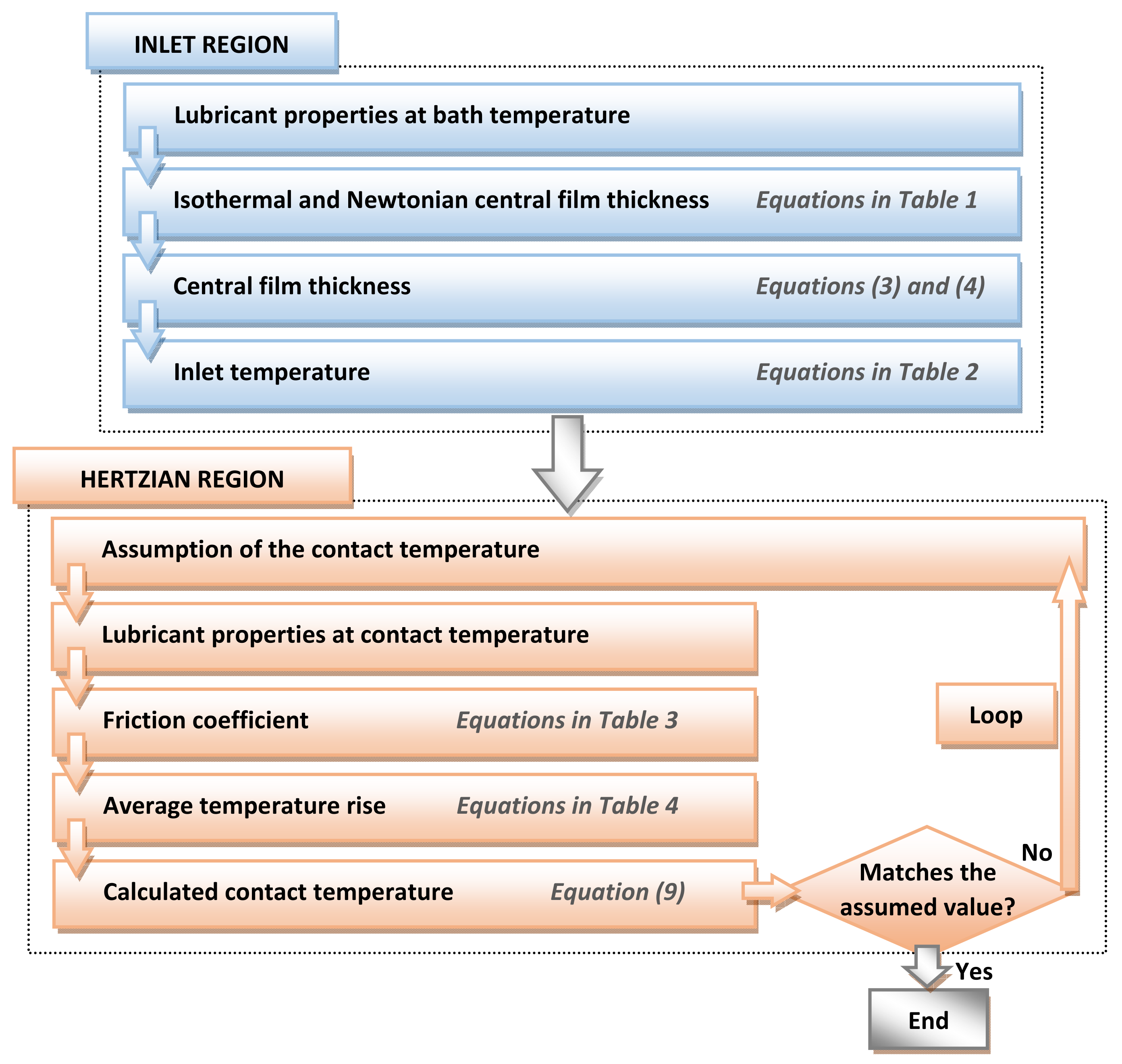
To calculate the friction coefficient in EHL, it is usual to only take into account the Couette component of the shear rate in the Hertzian region [54,55]. Therefore, the following expression can be used:
γ ˙ Δ u h
Taking into account the generalized viscosity of Equation (5), the shear stress in the Hertzian region can be obtained with Equation (8).
τ = η G γ ˙ η 1 + η G Δ u h 2 n 1 2 Δ u h
For the low-shear viscosity in Equation (6) and the Hertz pressure distribution, the integration of the shear stress equation in the contact area makes it possible to analytically obtain approximate expressions of the friction force in the most frequent cases [13,14]. The corresponding friction coefficient equations for line contact and point (circular or elliptical) contact are presented in Table 3.
In the expressions of Table 3, the viscous properties must be introduced at the contact temperature, i.e., the average temperature of the EHL film within the Hertzian contact region, since friction is mainly determined by the properties of the lubricant in this region [19,56].
The contact temperature can be found by taking into account two increments above the inlet temperature [13,14]: the average flash temperature rise of the surfaces and the average increase in the lubricant temperature with respect to the surfaces due to viscous heating. Consequently,
T c = T i n + Δ T f + Δ T L
The average flash temperature rise can be determined approximately with the expressions in Table 4 for a fast and simplified calculation. These expressions are derived from the results in reference [57] and they are valid for the whole range of surface velocities. The second increment can be found by considering that in EHL the main mechanism of heat transfer from the lubricant to the surfaces is conduction in the direction normal to the surfaces [5,15]. Thus, a simple heat balance provides the approximate equations that are also included in Table 4 [13,14]. Furthermore, the expressions in Table 4 can easily be modified to accommodate other contact geometries (for more details, see references [22,57,58]).

2.3. Methodology

It is commonly accepted that in EHL, a decoupling calculation of the lubricant film thickness and the friction coefficient can be performed [19,22]. As previously stated, the film thickness is essentially determined by the lubricant properties in the inlet region, whereas the friction depends mainly on the properties of the fluid film within the Hertzian contact region.
With this in mind, the methodology for applying the models is outlined in Figure 1. The formulae in Table 1 are used to obtain the Newtonian central film thickness with the lubricant properties at the bath temperature, leading to an isothermal result. Subsequently, thermal and shear-thinning corrections are taken into account, using Equations (3) and (4), to obtain the final value of the central thickness. In addition, Table 2 includes the expressions from which the inlet temperature can be obtained.
In contrast to film thickness, in friction calculations, the viscous properties of the lubricant are evaluated at the contact temperature. As this temperature is dependent on the friction coefficient, a simple iterative method is applied. From an initial assumption of the contact temperature, Table 3 contains the equations to obtain the friction coefficient at this temperature. This friction value is used to estimate the average temperature rise in the high-pressure contact region, with the formulae available in Table 4. Finally, Equation (9) gives the calculated contact temperature. The loop is repeated until the calculated temperature matches the assumed value, simultaneously finding the solution of both the friction coefficient and the contact temperature.

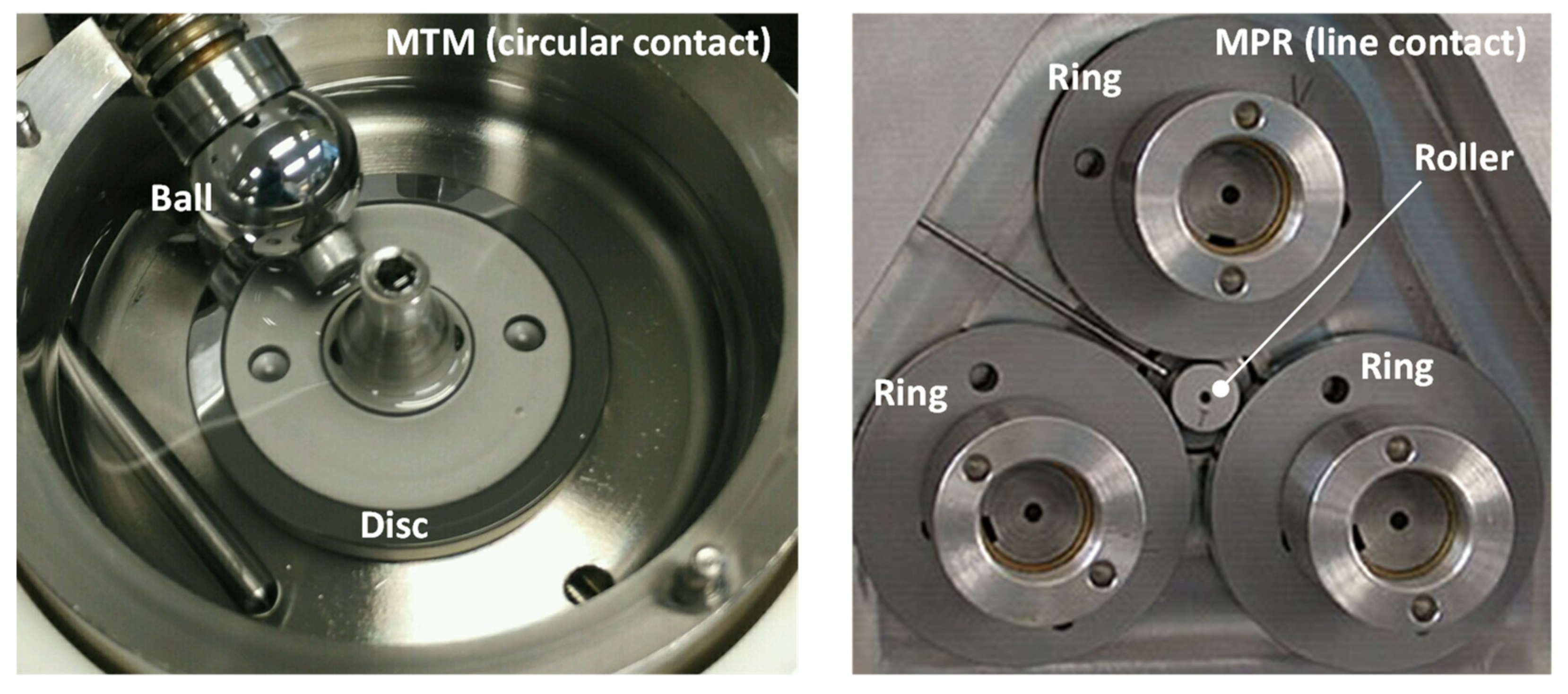
2.4. Experimentation

Friction coefficient measurements were performed on the MTM and MPR tribological test rigs developed by PCS Instruments (www.pcs-instruments.com, accessed on 1 May 2022), in order to compare the results with the models for circular and line contacts. In the MTM, the ball-on-disc configuration was used, with 9.525 mm radius steel balls and flat discs of steel and copper. In the MPR, a triple contact between steel discs was tested, consisting of three identical rings and a central roller, with radii of 27 and 6 mm, respectively, and with a contact length of 1 mm in the transverse direction. The setup in the MPR allows an evenly distributed normal load along the three contacts.
The MTM and the MPR allow testing under controlled conditions of bath temperature, normal load, average velocity and slide-to-roll ratio (SRR). The experimental setup is shown in Figure 2 and the mechanical and thermal properties of the materials are indicated in Table 5.
The test specimens were carefully polished and their combined RMS surface roughness was approximately 16 and 25 nm for the steel-steel and the steel-copper contacts, respectively.
All tests were performed with a polyalphaolefin (PAO-6) at a bath temperature of 80 °C under fully-flooded conditions. For this lubricant, some viscous properties are given in reference [15]: η0 = 7.36 mPa·s, α* = 9.0 GPa−1 at 80 °C; and η0 = 4.78 mPa·s, α* = 8.2 GPa−1 at 100 °C. In addition, according to references [13,14,59], the following values of the power-law exponent, shear modulus and thermal conductivity at 80 °C can be taken for the PAO-6: n = 0.81, G = 0.1 MPa and KL = 0.15 W/(mK).
Both MTM and MPR allow for a wide variety of operating conditions covering different lubrication regimes, and provide results with good repeatability [13,14]. The tests conducted include average velocities between 0.1 and 2.5 m/s and slide-to-roll ratios (SRRs) up to 150%. The types of configurations and the values of load selected are compiled in Table 6, along with the corresponding maximum Hertz pressures obtained with the formulae in Table 1.

3. Results and Discussion

The results of a friction test on the MTM for steel-steel contact with a load of 20 N and SRR of 50% are shown in Figure 3, as well as two modifications of this test: one increasing the load to 50 N and the other employing a copper disc instead of the steel disc.
The shape of the curves obtained is indicative of the existence of different lubrication regimes, from full film lubrication (EHL) for high average velocity to mixed lubrication when this velocity is reduced and an increase in friction is observed. The representation of the lambda ratio, calculated with Equation (1), allows for identifying the transition between lubrication regimes in each test when this ratio reaches a value of approximately 2.
As previously indicated, the steel-copper contact at 20 N in the MTM results in a maximum Hertz pressure of 0.67 GPa, which, for steel-steel specimens, increases to 0.83 GPa at 20 N and 1.12 GPa at 50 N. Comparing the results of the three tests for high average velocities, i.e., in the EHL regime, a friction increase with Hertz pressure is shown in Figure 3, mainly due to the piezoviscous response of the lubricant [60]. Furthermore, as the average velocity decreases and mixed lubrication is reached, the steel-copper contact gives rise to a more pronounced increase in friction, due to its lower lambda ratio and consequent earlier film rupture, in line with the results in references [61,62].

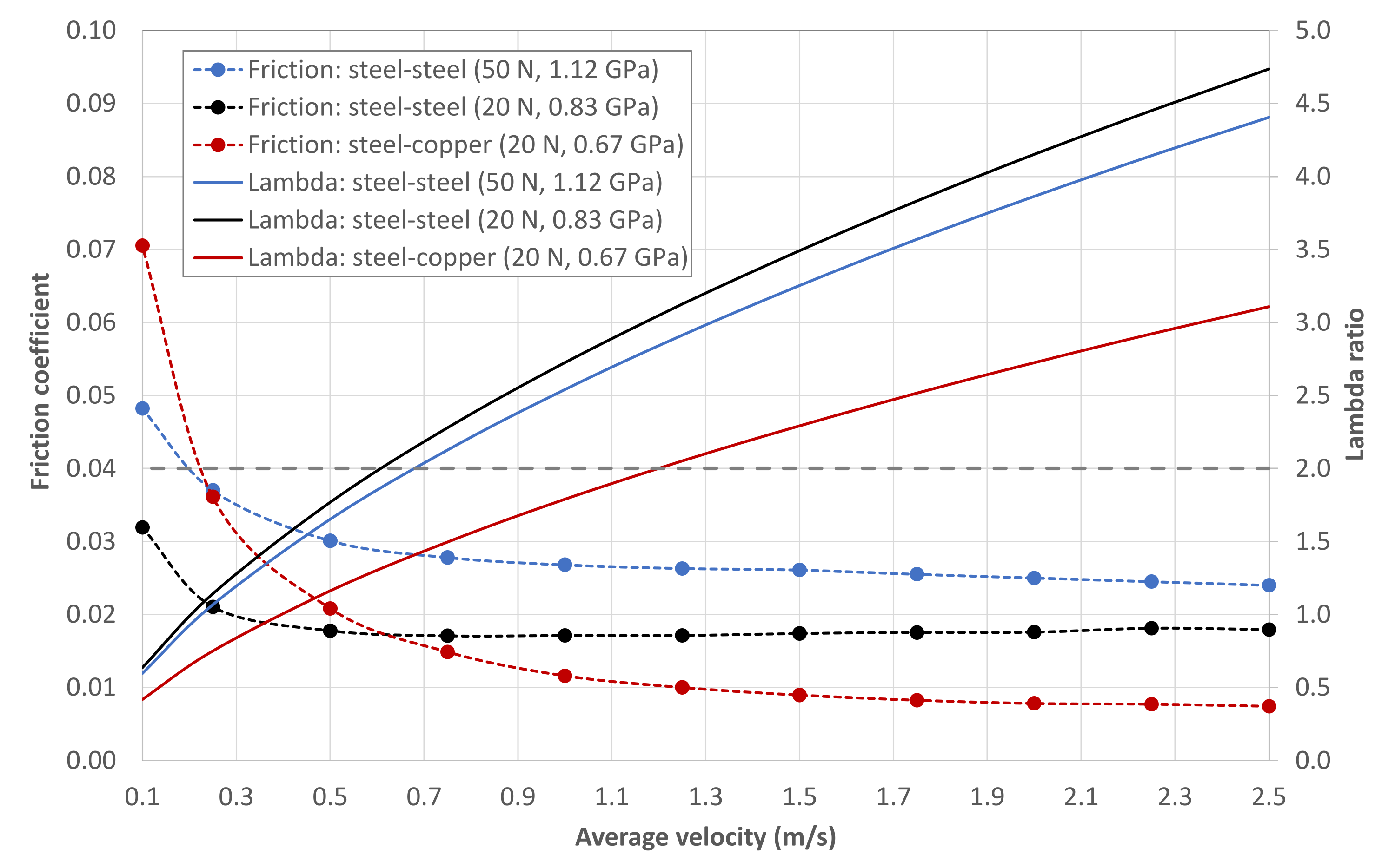
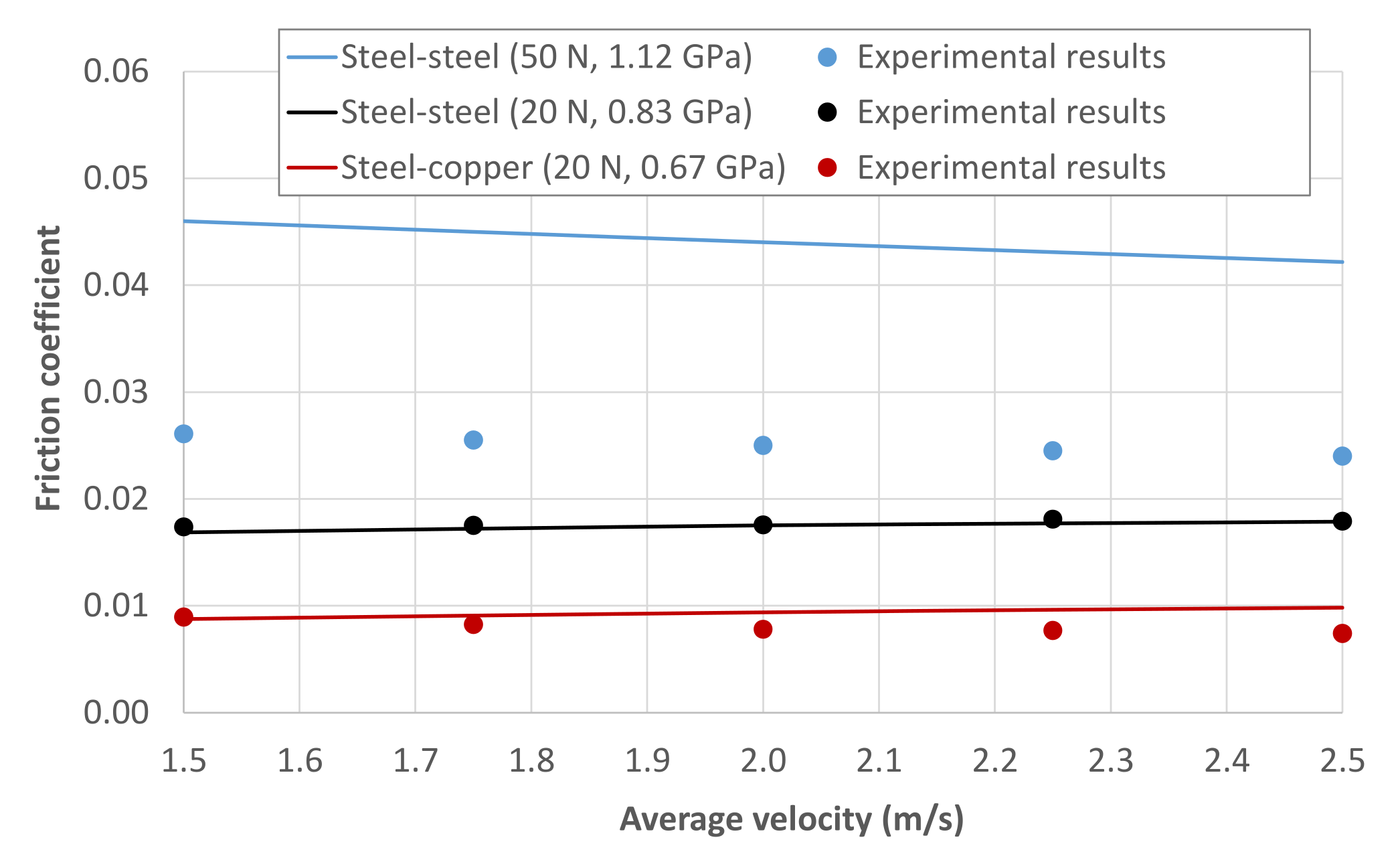
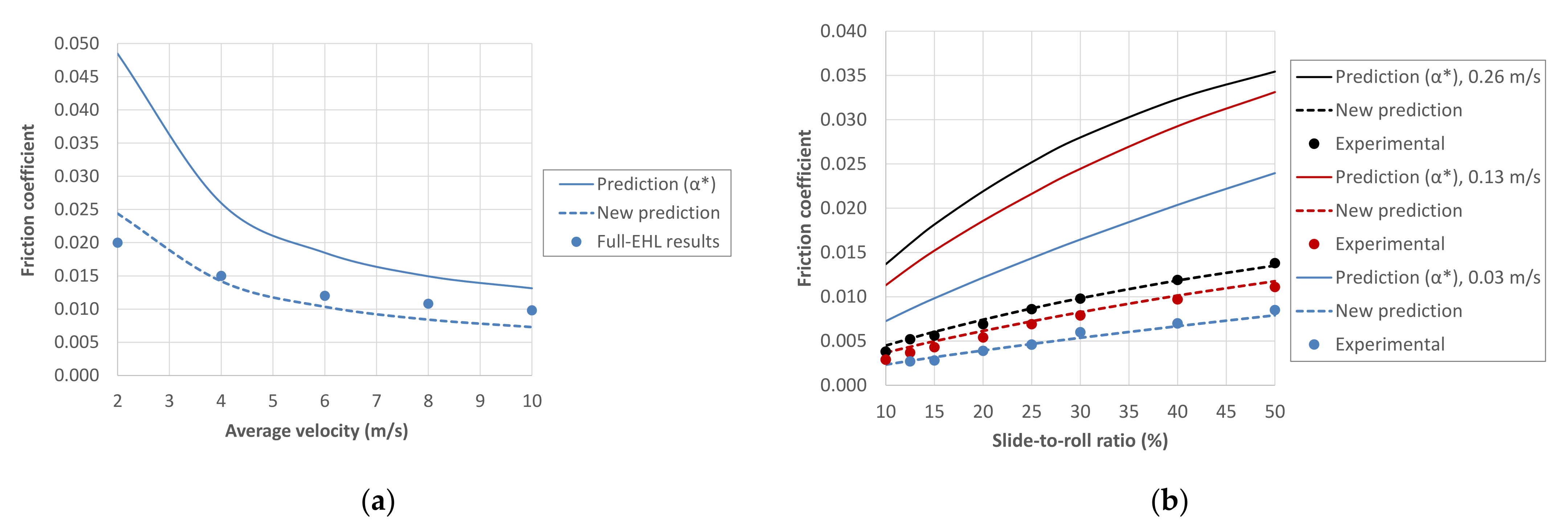
3.1. Initial Application of the Models

Considering the process described in the methodology, the friction models are applied to the PAO-6 in circular and line contacts under EHL conditions. According to the results in Figure 3, minimum average velocities of 1.5 m/s have been selected for the circular contact in order to ensure that the lambda ratio remains above 2. In Figure 4 and Figure 5, the estimates are compared with experimental data obtained in the MTM and MPR test rigs, as a function of the average velocity and SRR. Taking into account the Hertz pressure in each test, it can be seen that the predictions are mostly accurate for values of up to 0.86 GPa. On the contrary, when increasing the pressure to around 1.1 GPa, there is a clear tendency to overestimate the results for both circular and line contacts. This issue is related to the pressure dependence of the low-shear viscosity, as discussed in the following section.
The film thickness estimates corresponding to the friction results in Figure 4 and Figure 5 are compiled in Figure 6a,b, respectively. It can be seen that, even for low SRRs, the film thicknesses are lower than those obtained for the Newtonian and isothermal approach, which is in line with references [28,37]. The differences become greater both when increasing the average velocity at fixed SRR and when increasing the SRR at fixed average velocity, since both cases imply a proportional rise in the sliding velocity and more significant shear-thinning and thermal effects. In the results of Figure 6, the film thickness values are always more than twice the combined roughness, which ensures EHL conditions and negligible influence of the surface asperities on the friction coefficient [48,49,50]. Moreover, the MTM allows the electrical contact resistance (ECR) between the specimens to be measured during the tests. The ECR reading was usually 100%, which is indicative of full separation between the specimens.
The friction coefficient remains practically constant with the average velocity, as shown in Figure 4. In both theoretical and experimental results, a slight decreasing trend is found in the test at the highest Hertz pressure, which can be attributed to thermal effects [63]. The estimates of the contact temperature for the results in Figure 4 are presented in Figure 7a, where higher temperatures are observed as the pressure increases. However, the SRR value of 50% is relatively low and, consequently, the thermal effects are not very significant in any of these tests.
The variations in contact temperature are more clearly seen in the plot versus SRR shown in Figure 7b, which explain some results in Figure 5. For low SRRs, there is a rapid rise in the friction coefficient with SRR, which becomes less pronounced as SRR increases due to shear-thinning and thermal effects, in line with the results in references [54,61,64]. In tests at the highest pressures in Figure 5, there is even a decrease in friction for high SRRs, as the increase in temperature shown in Figure 7b leads to a significant drop in viscous properties. Comparing the tests with discs of different materials in Figure 5a, the higher thermal diffusivity of copper reduces the contact temperature, contributing to the friction curve having less variation in slope than that of the similar test with the steel disc.
In summary, the analytical approach provides estimates of great interest in EHL, such as the friction coefficient, film thickness and contact temperature. The results explain the general behaviour of circular and line contacts, taking shear-thinning and thermal effects into account. The calculations performed for the PAO-6 show a good accuracy in the prediction of friction for moderate values of the maximum Hertz pressure, of up to 0.86 GPa. However, at higher pressures, the friction values are overestimated. In the next section, some considerations are made to obtain more accurate predictions in different pressure ranges.

3.2. Influence of the Piezoviscous Response

As previously mentioned, the film thickness is established in the contact inlet zone, whereas the friction coefficient is determined by the conditions in the high-pressure contact zone. Therefore, it seems reasonable to use different values of the pressure-viscosity coefficient in each of these regions. Whereas the lubricant film thickness is calculated using the reciprocal asymptotic isoviscous pressure coefficient, using this same value in the exponent of Equation (6) may lead to incorrect predictions of the friction coefficient.
To illustrate the statement above, two oils of the same nature and very different viscosity have been selected, namely PAO-100 and PAO-650. The dependence of the low-shear viscosity on pressure for the PAO-100 is described by the Tait-Doolittle model [19], Equation (10), with the following parameters [65]: Koo = 11.804 GPa, K′o = 11.74, B = 3.811, αV = 0.0008 K−1, βK = 0.008655 K−1, VR/VR = 0.6193, ε = −0.00134 K−1, and ηR = 0.1803 Pa·s at TR = 70 °C. On the other hand, experimental measurements of the low-shear viscosity for the PAO-650 are given in reference [66].
η = η R exp B V R V R 1 + ε ( T T R ) 1 1 1 + K o ln 1 + p ( 1 + K o ) K o o exp ( β k T ) ( 1 + α V ( T T R ) ) V R V R 1 + ε ( T T R ) 1 1 V R V R
Hence, the reciprocal asymptotic isoviscous pressure coefficients can be computed using Equation (2). The results for the PAO-100 are 17.5 GPa−1 at 70 °C and 14.0 GPa−1 at 120 °C, whereas for the PAO-650 they are 20.1 GPa−1 at 20 °C and 14.8 GPa−1 at 75 °C. In addition, the variation of the pressure-viscosity coefficient shown in Figure 8 is obtained by fitting Equation (6) to the low-shear viscosity of these lubricants in pressure intervals of 0.2 GPa. The pressure-viscosity coefficient decreases with increasing pressure and moves away from the reciprocal asymptotic isoviscous pressure coefficient. If this variation is not taken into account, there is a general tendency to overestimate the viscosity and consequently also the friction coefficient. This issue becomes quite significant at high Hertz contact pressure, as can be seen in the results for the PAO-6 in Figure 4 and Figure 5.
Friction is primarily determined by the high-pressure rheology of the lubricant near the contact centre of the Hertzian region [56]. Therefore, to improve the accuracy of the models, it seems sensible to use the pressure-viscosity coefficient corresponding to the interval of the maximum Hertz contact pressure. The differences between using this value and the reciprocal asymptotic isoviscous pressure coefficient for the calculations in the Hertzian region are shown in Figure 9 for the PAO-100 and the PAO-650. It should be noted that all the estimates in this figure are obtained by using the reciprocal asymptotic isoviscous pressure coefficient for the calculations in the inlet region. The values of the power-law exponent and the shear modulus of the Carreau equation are given in reference [19]: n = 0.625, G = 1.5 MPa for the PAO-100; and n = 0.74, G = 0.031 MPa for the PAO-650. For both lubricants, a thermal conductivity of 0.15 W/(mK) has been taken as a typical value for a PAO [59]. The friction estimates are compared with full-EHL simulation results and experimental data provided in references [65,66] for these lubricants, which include different contact geometries and operating conditions. It can be seen that the results greatly improve when the pressure-viscosity coefficient for the maximum Hertz pressure interval is taken. In the cases in which maximum Hertz pressure falls at the endpoint of two pressure intervals, the mean of the two pressure-viscosity coefficients can be used.
In the same way, the pressure-viscosity coefficient of the PAO-6 at 100 °C and pressure close to 1.1 GPa can be derived from the experimental data in reference [67], resulting in approximately 7.4 GPa−1. If we assume a similar variation of this parameter at 80 °C, a rough estimate of the pressure-viscosity coefficient at 80 °C and 1.1 GPa can be obtained for the PAO-6, resulting in 8.3 GPa−1. The calculations in the Hertzian region using these new values lead to a significantly better agreement with the experimental data than that previously obtained at Hertz pressures of about 1.1 GPa, as demonstrated in Figure 10 and Figure 11.

3.3. Usefulness and Limitations of the Analytical Approach

The high complexity of the EHL problem limits any analytical approach to quantify film thickness and friction coefficient [68,69], especially if shear-thinning and thermal effects are taken into account. However, any EHL model must consider these effects in order to be considered realistic.
Simplifications introduced in the analytical formulation may decrease accuracy, as happens when approximating the piezoviscous response according to the exponential law (6) and taking the reciprocal asymptotic isoviscous pressure coefficient as the exponent. In fact, the discrepancy between the exponential law (6) and the experimental data obtained in viscometers is reported in references [69,70]. However, the use of models capable of representing the piezoviscous response more exactly, e.g., the Doolittle free-volume correlation along with the Tait equation of state [19,55], involves greater mathematical complexity and makes it extremely difficult to analytically derive formulae for predicting friction, such as those in Table 3.
Hence, in this article, we prefer to keep the formulation based on the simple exponential law, fitting the pressure-viscosity coefficient to the low-shear viscosity data in the pressure interval that includes the maximum Hertz pressure. The deviations between the friction estimates thus obtained for the PAO-100 and those calculated by numerical integration of the shear stress, Equation (8), for the Tait-Doolittle model (10) and the Hertz pressure distribution are presented in Figure 12. The comparison is approximately independent of the sliding velocity and film thickness, as these parameters affect the generalized viscosity in a similar way in the two friction calculation methods. The Hertz pressure values used to obtain this figure include the midpoint and the endpoints of each interval where the pressure-viscosity coefficient has been fitted in Figure 8. Similarly, higher Hertz pressures are also considered in Figure 12 for a more complete analysis.
The differences in the low-shear viscosity models result in sufficiently small deviations in the friction estimates under typical EHL pressures, as revealed in Figure 12, showing a reasonable accuracy of the formulation proposed in the article. Moreover, the analytical models enable easy and fast estimations of the friction coefficient, which can be obtained with the help of a simple spreadsheet. Additionally, the models provide information on the central film thickness and the average contact temperature. The modifications introduced in the equations to find this temperature enable even simpler and faster calculations than that proposed in previous references [13,14]. In contrast, the use of numerical methods is more difficult and time-consuming because it requires highly qualified personnel and specific software, and usually involves high computational cost.
Logically, the use of a simple exponential law, along with the pressure-viscosity coefficient corresponding to the interval of maximum Hertz pressure, implies an underestimation of the viscosity in the outermost parts of the Hertzian contact region at lower pressure. However, the models are not intended to completely describe the pressure dependence of the low-shear viscosity. They are aimed at enabling simplified calculations of the friction coefficient under EHL conditions, which is essentially determined by the high-pressure rheology of the lubricant near the contact centre of the Hertzian region. With the proposed approach, the friction formulae can be obtained in a fully analytical manner, which, together with the use of general equations to estimate the film thickness and the contact temperature, results in a broad scope of applicability of the models for EHL calculations.

4. Conclusions

Based on the EHL models previously developed by the authors, a simpler calculation of the thermal effects has been introduced, which can easily be modified to accommodate different contact geometries. The iterative method for estimating the friction coefficient has been described and the predictive potential of the models has been studied by comparison with full-EHL simulations and experimental data under different operating conditions.
The analysis of the influence of the pressure-viscosity coefficient on the results has shown the validity of the analytical models to predict friction when the piezoviscous response of the lubricant is more complex than a simple exponential law. In this case, the pressure-viscosity coefficient can be fitted to the low-shear viscosity at the maximum Hertz pressure.
In addition to the prediction of friction in EHL conjunctions with different contact geometries, the models also provide information on the film thickness and the temperature of the EHL film. This approach can be very useful in engineering applications, because it has a wide range of applicability and allows calculations to be performed quickly, easily and with reasonable accuracy, without the need for tedious computational methods.
It is worth noting that the analytical approach has some limitations when compared to the numerical models:
  • The film thickness formulae employed were obtained by curve fitting data over ranges of operating parameters. Therefore, outside these ranges, deviations in the predictions may be expected. However, the calculation process proposed in the article remains valid for other film thickness formulae, which could be either more general equations or expressions adapted to the range of operating conditions in each case.
  • The analytical deduction of friction formulae becomes increasingly difficult as more complex rheological models are considered, such as when using free volume correlations for the low-shear viscosity. To overcome this issue, a simple exponential law can be considered and the values of the pressure-viscosity coefficient can be fitted to the real piezoviscous response.
  • Although the use of equations for the central film thickness and the average contact temperature provides very useful information, the analytical approach cannot predict the film thickness and temperature distributions within the EHL contact.
  • As a consequence of all the simplifications introduced, less accurate results may be expected in any analytical approach. However, the formulation proposed can capture the essential features of the EHL contacts and exhibits a reasonably good predictive potential.
Furthermore, the following future developments could improve the applicability of the analytical approaches:
  • The deduction of new film thickness equations applicable in a more general way. They may be obtained from EHL solutions in a broader range of operating conditions by means of curve-fitted regression formulae. Similarly, more general film thickness correction factors for shear-thinning and thermal effects can also be derived.
  • The consideration of other effects for an improved formulation, such as transient conditions or starvation. Although they would complicate the development of purely analytical models, these effects could be considered by using machine learning algorithms or semi-analytical approaches, such as those based on the Reynolds-Carreau equations, integrated into the calculation process described in the article.
  • A methodology similar to that proposed in the present article may also be applied to other geometries of interest, such as the elliptical contact. To this end, some references and indications are provided in Section 2.

Author Contributions

Conceptualization, J.E.O. and E.d.l.G.O.; Methodology, J.E.O., E.d.l.G.O. and E.C.T.; Software, J.E.O. and E.C.T.; Validation, J.E.O., E.C.T., F.F.M. and R.W.C.U.; Investigation, J.E.O., E.d.l.G.O., E.C.T., F.F.M. and R.W.C.U.; Resources, J.E.O.; Original draft preparation, J.E.O.; Review and editing, E.d.l.G.O. and E.C.T. All authors have read and agreed to the published version of the manuscript.

Funding

This research received no external funding.

Institutional Review Board Statement

Not applicable.

Informed Consent Statement

Not applicable.

Data Availability Statement

Not applicable.

Acknowledgments

The authors would like to thank Ramsey and Carmen Gohar for their friendship and kindness. We are also grateful for Ramsey’s outstanding and inspiring contributions to Tribology. In addition, we would like to acknowledge the support of the Repsol Technology Lab. (Móstoles, Spain).

Conflicts of Interest

The authors declare no conflict of interest.

Nomenclature

acontact half-width (or radius for circular point contact), m
BDoolittle parameter
E1, E2Young’s modulus of the contacting bodies, Pa
E’ reduced   Young s   modulus ,   Pa :   1 E = 1 2 1 ν 1 2 E 1 + 1 ν 2 2 E 2
Gshear modulus of the lubricant, Pa
hcentral film thickness, m
hNNewtonian central film thickness, m
K1, K2thermal conductivity of the contacting bodies, W/(mK)
KLthermal conductivity of the lubricant, W/(mK)
K′opressure rate of change of isothermal bulk modulus at p = 0
Kooisothermal bulk modulus at zero absolute temperature and p = 0, Pa
LTthermal loading factor
npower-law exponent
ppressure, Pa
pHHertz (maximum) pressure, Pa
Rreduced radius of curvature, m: R = 1 R 1 + 1 R 1 1
R1,R2radii of the contacting surfaces, m
Rqcombined RMS surface roughness, m
SRR slide - to - roll   ratio ,   % :   S R R = Δ u u m 100
Tabsolute temperature in the Tait-Doolittle equation, K
Tblubricant bath temperature, °C
Tccontact temperature, °C
Tininlet temperature, °C
TRreference temperature in the Tait-Doolittle equation, K
u1, u2velocities of the contacting surfaces, m/s
umaverage velocity or rolling velocity, m/s
VRvolume at reference temperature and p = 0, m3
V∞Roccupied volume at reference temperature and p = 0, m3
Wnormal load, N
W/Lnormal load per unit length, N/m
αpressure-viscosity coefficient, Pa−1
α*reciprocal asymptotic isoviscous pressure coefficient, Pa−1
αVthermal expansivity, K−1
βtemperature-viscosity coefficient, K−1
βktemperature coefficient of isothermal bulk modulus at p = 0, K−1
γ ˙ shear rate, s−1
ΔTfaverage flash temperature rise, °C
ΔTLaverage temperature rise with respect to the surfaces due to viscous heating, °C
Δusliding velocity, m/s
εoccupied volume thermal expansivity, K−1
ηlow-shear viscosity, Pa·s
η0low-shear viscosity at p = 0, Pa·s
ηGgeneralized viscosity, Pa·s
ηRlow-shear viscosity at reference temperature and p = 0, Pa·s
λspecific lubricant film thickness or lambda ratio
μfriction (or traction) coefficient
ν1, ν2Poisson ratio of the contacting bodies
ρ1, ρ2density of the contacting bodies, kg/m3
σ1, σ2specific heat of the contacting bodies, J/(kgK)
τshear stress, Pa
φTthermal film thickness reduction factor

References

  1. Dowson, D. History of Tribology, 2nd ed.; Professional Engineering Publishing: London, UK, 1998. [Google Scholar]
  2. Echávarri, J.; De la Guerra, E.; Chacón, E. Tribology: A historical overview of the relation between theory and application. In A Bridge between Conceptual Frameworks: Sciences, Society and Technology Studies; Pisano, R., Ed.; Springer: Dordrecht, The Netherlands, 2015. [Google Scholar]
  3. Johns-Rahnejat, P.M.; Karami, G.; Aini, R.; Rahnejat, H. Fundamentals and advances in elastohydrodynamics: The role of Ramsey Gohar. Lubricants 2021, 9, 120. [Google Scholar] [CrossRef]
  4. Stachowiak, G.W. How tribology has been helping us to advance and to survive. Friction 2017, 5, 233–247. [Google Scholar] [CrossRef] [Green Version]
  5. Habchi, W.; Eyheramendy, D.; Bair, S.; Vergne, P. Thermal elastohydrodynamic lubrication of point contacts using a Newtonian/Generalized Newtonian lubricant. Tribol. Lett. 2008, 30, 41–52. [Google Scholar] [CrossRef]
  6. Carli, M.; Sharif, K.J.; Ciulli, E.; Evans, H.P.; Snidle, R.W. Thermal point contact EHL analysis of rolling sliding contacts with experimental comparison showing anomalous film shapes. Tribol. Int. 2009, 42, 517–525. [Google Scholar] [CrossRef]
  7. Echávarri, J.; de la Guerra, E.; Chacón, E.; Lafont, P.; Díaz, A.; Munoz-Guijosa, J.M.; Muñoz, J.L. Artificial neural network approach to predict the lubricated friction coefficient. Lubr. Sci. 2014, 26, 141–162. [Google Scholar] [CrossRef]
  8. Olver, A.V.; Spikes, H.A. Prediction of traction in elastohydrodynamic lubrication. Proc. Inst. Mech. Eng. Part J J. Eng. Tribol. 1998, 212, 321–332. [Google Scholar] [CrossRef]
  9. Morales-Espejel, G.E.; Wemekamp, A.W. An engineering approach on sliding friction in full-film, heavily loaded lubricated contacts. Proc. Inst. Mech. Eng. Part J J. Eng. Tribol. 2004, 218, 513–528. [Google Scholar] [CrossRef]
  10. Masjedi, M.; Khonsari, M.M. An engineering approach for rapid evaluation of traction coefficient and wear in mixed EHL. Tribol. Int. 2015, 92, 184–190. [Google Scholar] [CrossRef]
  11. Paouris, L.; Rahmani, R.; Theodossiades, S.; Rahnejat, H.; Hunt, G.; Barton, W. An analytical approach for prediction of elastohydrodynamic friction with inlet shear heating and starvation. Tribol. Lett. 2016, 64, 10. [Google Scholar] [CrossRef] [Green Version]
  12. Shirzadegan, M.; Larsson, R.; Almqvist, A. A low degree of freedom approach for prediction of friction in finite EHL line contacts. Tribol. Int. 2017, 115, 628–639. [Google Scholar] [CrossRef]
  13. Echávarri, J.; Lafont, P.; Chacón, E.; de la Guerra, E.; Díaz, A.; Munoz-Guijosa, J.M.; Muñoz, J.L. Analytical model for predicting friction coefficient in point contacts with thermal elastohydrodynamic lubrication. Proc. Inst. Mech. Eng. Part J J. Eng. Tribol. 2011, 225, 181–191. [Google Scholar] [CrossRef]
  14. Echávarri, J.; de la Guerra, E.; Chacón, E.; Díaz, A.; Munoz-Guijosa, J.M. Analytical model for predicting friction in line contacts. Lubr. Sci. 2016, 28, 189–205. [Google Scholar] [CrossRef] [Green Version]
  15. De la Guerra, E.; Echávarri, J.; Chacón, E.; del Río, B. A thermal resistances-based approach for thermal-elastohydrodynamic calculations in point contacts. Proc. Inst. Mech. Eng. Part C J. Mech. Eng. Sci. 2018, 232, 2088–2102. [Google Scholar] [CrossRef]
  16. Stachowiak, G.W.; Batchelor, A.W. Engineering Tribology; Elsevier: Oxford, UK, 2005. [Google Scholar]
  17. Gohar, R. Elastohydrodynamics; Ellis Horwood Limited: Chichester, UK, 1988. [Google Scholar]
  18. Gohar, R.; Rahnejat, H. Fundamentals of Tribology, 3rd ed.; World Scientific Publishing: London, UK, 2018. [Google Scholar]
  19. Bair, S. High Pressure Rheology for Quantitative Elastohydrodynamics; Elsevier: Burlington, MA, USA, 2007. [Google Scholar]
  20. Marian, M.; Tremmel, S. Current trends and applications of machine learning in tribology—A review. Lubricants 2021, 9, 86. [Google Scholar] [CrossRef]
  21. Marian, M.; Mursak, J.; Bartz, M.; Profito, F.J.; Rosenkranz, A.; Wartzack, S. Predicting EHL film thickness parameters by machine learning approaches. Friction 2022. [Google Scholar] [CrossRef]
  22. Spikes, H. Basics of EHL for practical application. Lubr. Sci. 2015, 27, 45–67. [Google Scholar] [CrossRef] [Green Version]
  23. Hamrock, B.J. Fundamentals of Fluid Film Lubrication; McGraw-Hill: New York, NY, USA, 1994. [Google Scholar]
  24. Dowson, D.; Toyoda, S. A central film thickness formula for elastohydrodynamic line contacts. In Elastohydrodynamics and Related Topics; Dowson, D., Taylor, C.M., Godet, M., Berthe, D., Eds.; Mechanical Engineering Publications: Leeds, UK, 1978. [Google Scholar]
  25. Pan, P.; Hamrock, B.J. Simple formulas for performance parameters used in elastohydrodynamically lubricated line contacts. ASME J. Tribol. 1989, 111, 246–251. [Google Scholar] [CrossRef]
  26. Hamrock, B.J.; Dowson, D. Ball bearing lubrication: The Elastohydrodynamics of Elliptical Contacts; Wiley-lnterscience: New York, NY, USA, 1981. [Google Scholar]
  27. Chaomleffel, J.P.; Dalmaz, G.; Vergne, P. Experimental results and analytical film thickness predictions in EHD rolling point contacts. Tribol. Int. 2007, 40, 1543–1552. [Google Scholar] [CrossRef]
  28. Katyal, P.; Kumar, P. New central film thickness equation for shear thinning lubricants in elastohydrodynamic lubricated rolling/sliding point contact conditions. ASME J. Tribol. 2014, 136, 041504. [Google Scholar] [CrossRef]
  29. Moes, H. Optimum Similarity Analysis with applications to Elastohydrodynamic Lubrication. Wear 1992, 159, 57–66. [Google Scholar] [CrossRef] [Green Version]
  30. Moes, H. Lubrication and Beyond; Lecture Notes, Code 115531; University of Twente: Enschede, The Netherlands, 2000. [Google Scholar]
  31. Nijenbanning, G.; Venner, C.H.; Moes, H. Film thickness in elastohydrodynamically lubricated elliptic contacts. Wear 1994, 176, 217–229. [Google Scholar] [CrossRef] [Green Version]
  32. Katyal, P.; Kumar, P. Central film thickness formula for shear thinning lubricants in EHL point contacts under pure rolling. Tribol. Int. 2012, 48, 113–121. [Google Scholar] [CrossRef]
  33. Marian, M.; Bartz, M.; Wartzack, S.; Rosenkranz, A. Non-dimensional groups, film thickness equations and correction factors for elastohydrodynamic lubrication: A review. Lubricants 2020, 8, 95. [Google Scholar] [CrossRef]
  34. Sivayogan, G.; Rahmani, R.; Rahnejat, H. Transient non-Newtonian elastohydrodynamics of rough meshing hypoid gear teeth subjected to complex contact kinematics. Tribol. Int. 2022, 167, 107398. [Google Scholar] [CrossRef]
  35. Habchi, W.; Bair, S.; Qureshi, F.; Covitch, M. A film thickness correction formula for double-Newtonian shear-thinning in rolling EHL circular contacts. Tribol. Lett. 2013, 50, 59–66. [Google Scholar] [CrossRef]
  36. Anuradha, P.; Kumar, P. New film thickness formula for shear thinning fluids in thin film elastohydrodynamic lubrication line contacts. Proc. Inst. Mech. Eng. Part J J. Eng. Tribol. 2011, 225, 173–179. [Google Scholar] [CrossRef]
  37. De la Guerra, E.; Echávarri, J.; Sánchez, A.; Chacón, E.; del Río, B. Film thickness formula for thermal EHL line contact considering a new Reynolds–Carreau equation. Tribol. Lett. 2018, 66, 31. [Google Scholar] [CrossRef] [Green Version]
  38. Habchi, W.; Vergne, P.; Bair, S.; Andersson, O.; Eyheramendy, D.; Morales-Espejel, G.E. Influence of pressure and temperature dependence of thermal properties of a lubricant on the behavior of circular TEHD contacts. Tribol. Int. 2010, 43, 1842–1850. [Google Scholar] [CrossRef]
  39. Habchi, W.; Bair, S.; Vergne, P. On friction regimes in quantitative elastohydrodynamics. Tribol. Int. 2013, 58, 107–117. [Google Scholar] [CrossRef]
  40. Bair, S. A rough shear thinning correction for EHD film thickness. STLE Tribol. Trans. 2004, 47, 361–365. [Google Scholar] [CrossRef]
  41. Bair, S. Shear thinning correction for rolling/sliding elastohydrodynamic film thickness. Proc. Inst. Mech. Eng. Part J J. Eng. Tribol. 2005, 219, 69–74. [Google Scholar] [CrossRef]
  42. Cheng, H.S. Calculations of Elastohydrodynamic Film Thickness in High Speed Rolling and Sliding Contacts; Technical Report, MTI-67TR24; Mechanical Technology, Inc.: Albany, NY, USA, 1967. [Google Scholar]
  43. Gupta, P.K.; Cheng, H.S.; Forster, N.H.; Schrand, J.B. Viscoelastic effects in MIL-L-7808-type lubricant. Part I: Analytical formulation. Tribol. Trans. 1992, 35, 269–274. [Google Scholar] [CrossRef]
  44. Jubault, I.; Molimard, J.; Lubrecht, A.A.; Mansot, J.L.; Vergne, P. In situ pressure and film thickness measurements in rolling/sliding lubricated point contacts. Tribol. Lett. 2003, 15, 421–429. [Google Scholar] [CrossRef]
  45. De la Guerra, E.; Echávarri, J.; Sánchez, A.; Chacón, E. Film thickness predictions for line contact using a new Reynolds-Carreau equation. Tribol. Int. 2015, 82, 133–141. [Google Scholar] [CrossRef]
  46. Stribeck, R. Ball bearings for various loads. Trans. ASME 1907, 29, 420–463. [Google Scholar]
  47. Hersey, M.D. The laws of lubrication of horizontal journal bearings. J. Wash. Acad. Sci. 1914, 19, 542–552. [Google Scholar]
  48. Zhu, D.; Hu, Y. A computer program package for the prediction of EHL and mixed lubrication characteristics, friction, subsurface stresses and flash temperatures based on measured 3-D surface roughness. Tribol. Trans. 2001, 44, 383–390. [Google Scholar] [CrossRef]
  49. Castro, J.; Seabra, J. Coefficient of friction in mixed film lubrication: Gears versus twin-discs. Proc. Inst. Mech. Eng. Part J J. Eng. Tribol. 2007, 221, 399–411. [Google Scholar] [CrossRef]
  50. Brandão, A.; Seabra, J.; Castro, J. Surface initiated tooth flank damage. Part I: Numerical model. Wear 2010, 268, 1–12. [Google Scholar] [CrossRef]
  51. Vergne, P. Super low traction under EHD and mixed lubrication regimes. In Superlubricity; Erdemir, A., Martin, J.M., Eds.; Elsevier: Amsterdam, The Netherlands, 2007. [Google Scholar] [CrossRef]
  52. Chittenden, R.J.; Dowson, D.; Dunn, J.F.; Taylor, C.M. A theoretical analysis of the isothermal elastohydrodynamic lubrication of concentrated contacts II. General Case, with lubricant entrainment along either principal axis of the Hertzian contact ellipse or at some intermediate angle. Proc. R. Soc. Lond. A 1985, 397, 271–294. [Google Scholar] [CrossRef]
  53. Carreau, P.J. Rheological equations from molecular network theories. Trans. Soc. Rheol. 1972, 16, 99–127. [Google Scholar] [CrossRef]
  54. Johnson, K.L.; Tevaarwerk, J.L. Shear behaviour of elastohydrodynamic oil films. Proc. R. Soc. Lond. A 1977, 356, 215–236. [Google Scholar] [CrossRef]
  55. Kumar, P.; Anuradha, P.; Khonsari, M.M. Some important aspects of thermal elastohydrodynamic lubrication. Proc. Inst. Mech. Eng. Part C J. Mech. Eng. Sci. 2010, 224, 2588–2598. [Google Scholar] [CrossRef]
  56. Bair, S. Is it possible to extract the pressure dependence of low-shear viscosity from EHL friction? Revised May, 2020. Tribol. Int. 2020, 151, 106454. [Google Scholar] [CrossRef]
  57. Tian, X.; Kennedy, F.E., Jr. Maximum and average flash temperatures in sliding contacts. ASME. J. Tribol. 1994, 116, 167–174. [Google Scholar] [CrossRef]
  58. Bhushan, B. Modern Tribology Handbook. Volume One: Principles of Tribology; CRC Press: Boca Raton, FL, USA, 2000. [Google Scholar]
  59. Larsson, R.; Andersson, O. Lubricant thermal conductivity and heat capacity under high pressure. Proc. Inst. Mech. Eng. Part J J. Eng. Tribol. 2000, 214, 337–342. [Google Scholar] [CrossRef]
  60. Lafont, P.; Echávarri, J.; Sánchez-Peñuela, J.B.; Muñoz, J.L.; Díaz, A.; Munoz-Guijosa, J.M.; Lorenzo, H.; Leal, P.; Muñoz, J. Models for predicting friction coefficient and parameters with influence in elastohydrodynamic lubrication. Proc. Inst. Mech. Eng. Part J J. Eng. Tribol. 2009, 223, 949–958. [Google Scholar] [CrossRef] [Green Version]
  61. Hansen, J.; Björling, M.; Larsson, R. Mapping of the lubrication regimes in rough surface EHL contacts. Tribol. Int. 2019, 131, 637–651. [Google Scholar] [CrossRef]
  62. Bellón, I.; de la Guerra, E.; Echávarri, J.; Chacón, E.; Fernández, I.; Santiago, J.A. Individual and combined effects of introducing DLC coating and textured surfaces in lubricated contacts. Tribol. Int. 2020, 151, 106440. [Google Scholar] [CrossRef]
  63. Lafountain, A.R.; Johnston, G.J.; Spikes, H.A. The elastohydrodynamic traction of synthetic base oil blends. Tribol. Trans. 2001, 44, 648–656. [Google Scholar] [CrossRef]
  64. Vengudusamy, B.; Enekes, C.; Spallek, R. EHD friction properties of ISO VG 320 gear oils with smooth and rough surfaces. Friction 2020, 8, 164–181. [Google Scholar] [CrossRef] [Green Version]
  65. Kumar, P.; Khonsari, M.M. Traction in EHL line contacts using free-volume pressure–viscosity relationship with thermal and shear-thinning effects. J. Tribol. 2009, 131, 011503. [Google Scholar] [CrossRef]
  66. Bair, S.; Vergne, P.; Querry, M. A unified shear-thinning treatment of both film thickness and traction in EHD. Tribol. Lett. 2005, 18, 145–152. [Google Scholar] [CrossRef] [Green Version]
  67. Nakamura, Y.; Hiraiwa, S.; Suzuki, F.; Matsui, M. High-Pressure Viscosity Measurements of Polyalphaorefins at Elevated Temperature. Tribol. Online 2016, 11, 444–449. [Google Scholar] [CrossRef] [Green Version]
  68. Bair, S. The unresolved definition of the pressure-viscosity coefficient. Sci. Rep. 2022, 12, 3422. [Google Scholar] [CrossRef]
  69. Spikes, H.; Jie, Z. History, origins and prediction of elastohydrodynamic friction. Tribol. Lett. 2014, 56, 1–25. [Google Scholar] [CrossRef] [Green Version]
  70. Bair, S. Pressure-viscosity response in the inlet zone for quantitative elastohydrodynamics. Tribol. Int. 2016, 97, 272–277. [Google Scholar] [CrossRef] [Green Version]
Figure 1. Flow chart for calculating film thickness, temperature and friction coefficient.
Lubricants 10 00141 g001
Figure 2. MTM and MPR test rigs.
Lubricants 10 00141 g002
Figure 3. Friction test results and calculated lambda ratio for each test. Ball-on-disc contact lubricated with PAO-6 at Tb = 80 °C and SRR = 50%.
Lubricants 10 00141 g003
Figure 4. Comparison of the models with experimental results. Ball-on-disc contact lubricated with PAO-6 at Tb = 80 °C and SRR = 50%.
Lubricants 10 00141 g004
Figure 5. Comparison of the models with experimental results for the PAO-6 oil at Tb = 80 °C: (a) Ball-on-disc contact at um = 2 m/s; (b) Triple contact between steel discs at um = 2.5 m/s.
Lubricants 10 00141 g005
Figure 6. Estimated film thickness for the results in: (a) Figure 4; (b) Figure 5. The dashed lines denote the Newtonian and isothermal result.
Lubricants 10 00141 g006
Figure 7. Estimated contact temperature for the results in: (a) Figure 4; (b) Figure 5.
Lubricants 10 00141 g007
Figure 8. Low-shear viscosity of the PAO-100 [65] and PAO-650 [66] oils at different temperatures and resulting pressure-viscosity coefficients in each interval of 0.2 GPa. Numbers in italics indicate the viscosity at ambient pressure.
Lubricants 10 00141 g008
Figure 9. Influence of the pressure-viscosity coefficient on the prediction of the friction coefficient: (a) Steel-steel line contact lubricated with PAO-100 at Tb = 70 °C, pH = 1 GPa and SRR = 100%; (b) Steel ball on glass disc, lubricated with PAO-650 at Tb = 75 °C, pH = 0.53 GPa and um = 0.03, 0.13 and 0.26 m/s. (For more details, see references [65,66]).
Lubricants 10 00141 g009
Figure 10. New prediction for the results at highest pressure in Figure 4. Steel ball on steel disc contact lubricated with PAO-6 at Tb = 80 °C, SRR = 50% and W = 50 N (pH = 1.12 GPa).
Lubricants 10 00141 g010
Figure 11. New prediction for the results at highest pressures in Figure 5: (a) Steel ball on steel disc contact lubricated with PAO-6 at Tb = 80 °C, um = 2 m/s and W = 50 N (pH = 1.12 GPa); (b) Triple contact between steel discs lubricated with PAO-6 at Tb = 80 °C, um = 2.5 m/s and W = 150 N (pH = 1.06 GPa).
Lubricants 10 00141 g011
Figure 12. Friction calculated with the methodology proposed in the article (µF) versus numerical integration of the Tait-Doolittle equation (µTD) for the PAO-100, Δu = 1 m/s and h = 80 nm. Percentage deviations calculated as the absolute value of 100(µF µTD)/µTD.
Lubricants 10 00141 g012
Table 1. Classical central film thickness formulae and Hertzian contact parameters. The film thickness formula for each type of geometry is expressed both as a function of non-dimensional groups and in terms of dimensional parameters.
Type of GeometryNewtonian Film ThicknessHertzian Parameters
Circular contact h N R = 1.90 η 0 u m E R 0.67 α * E 0.53 W E R 2 0.067
Equivalently :   h N = 1.55 α * 0.53 η 0 u m 0.67 E 0.061 R 0.33 p H 0.201
p H = 3 W 2 π a 2 a = 3 W R 2 E 1 / 3
Line contact h N R = 2.922 η 0 u m E R 0.692 α * E 0.47 W / L E R 0.166
Equivalently :   h N = 2.154 α * 0.47 η 0 u m 0.692 E 0.110 R 0.308 p H 0.332
p H = 2 ( W / L ) π a a = 8 ( W / L ) R π E 1 / 2
Table 2. Equations for estimating the inlet temperature.
Type of GeometryEquation
Circular contact η 0 ( T i n ) 0.67 α * ( T i n ) 0.53 = φ T η 0 ( T b ) 0.67 α * ( T b ) 0.53
Line contact η 0 ( T i n ) 0.692 α * ( T i n ) 0.47 = φ T η 0 ( T b ) 0.692 α * ( T b ) 0.47
Table 3. Friction coefficient formulae for EHL [13,14].
GeometryFormula
Point
contact
μ = 3 η 0 Δ u h n G 1 n p H exp ( n α p H ) n α p H 1 1 n α p H + 1 n α p H 2
Line
contact
μ = η 0 Δ u h n G 1 n p H 4 π + n α p H 3 2 + 3 2 exp n α p H 1 2 3 4 + exp n α p H 2 2 + 2 3 2 exp n α p H 1 2 + 3 4
Table 4. Temperature rise in the high-pressure contact region.
GeometryAverage Temperature Rise Formulae
Circular contact Δ T f = 0.37 μ W Δ u / a K 1 ( 1.74 K 1 + a u 1 ρ 1 σ 1 ) + K 2 ( 1.74 K 2 + a u 2 ρ 2 σ 2 ) Δ T L = μ W h Δ u 8 π a 2 K L
Line
Contact
Δ T f = 0.53 μ ( W / L ) Δ u K 1 ( 0.90 K 1 + a u 1 ρ 1 σ 1 ) + K 2 ( 0.90 K 2 + a u 2 ρ 2 σ 2 ) Δ T L = μ ( W / L ) h Δ u 16 a K L
Table 5. Properties of the tested materials [13].
PropertySteelCopper
Young’s modulus, GPa210117
Poisson ratio0.300.34
Thermal conductivity, W/(mK)41385
Density, kg/m378508913
Specific heat, J/(kgK)418398
Table 6. Load and Hertz (maximum) pressure in each test.
Test Rig and Type of ContactMaterialsLoad, NHertz Pressure, GPa
MTM, ball-on-discsteel-copper200.67
steel-steel200.83
steel-steel501.12
MPR, triple-discsteel-steel1000.86
steel-steel1501.06
Publisher’s Note: MDPI stays neutral with regard to jurisdictional claims in published maps and institutional affiliations.

