Hot Metal Temperature Forecasting at Steel Plant Using Multivariate Adaptive Regression Splines


Polytechnic School of Engineering, University of Oviedo, 33204 Gijón, Spain
*
Author to whom correspondence should be addressed.
Metals 2020, 10(1), 41; https://0-doi-org.brum.beds.ac.uk/10.3390/met10010041
Submission received: 3 December 2019
/
Revised: 18 December 2019
/
Accepted: 20 December 2019
/
Published: 24 December 2019
Abstract
:Steelmaking has been experiencing continuous challenges and advances concerning process methods and control models. Integrated steelmaking begins with the hot metal, a crude liquid iron that is produced in the blast furnace (BF). The hot metal is then pre-treated and transferred to the basic lined oxygen furnace (BOF) for refining, experiencing a non-easily predictable temperature drop along the BF–BOF route. Hot metal temperature forecasting at the BOF is critical for the environment, productivity, and cost. An improved multivariate adaptive regression splines (MARS) model is proposed for hot metal temperature forecasting. Selected process variables and past temperature measurements are used as predictors. A moving window approach for the training dataset is chosen to avoid the need for periodic re-tuning of the model. There is no precedent for the application of MARS techniques to BOF steelmaking and a comparable temperature forecasting model of the BF–BOF interface has not been published yet. The model was trained, tested, and validated using a plant process dataset with 12,195 registers, covering one production year. The mean absolute error of predictions is 11.2 °C, which significantly improves those of previous modelling attempts. Moreover, model training and prediction are fast enough for a reliable on-line process control.
1. Introduction
Through the last decades, the steel industry has been facing increasing challenges for improved productivity and quality with optimum cost and minimum impact on the environment. These requirements have been met by advances in production methods and process models [1]. Temperature is one of the most critical variables to be controlled along the process route and a required input for almost any control model in steelmaking operations.
Steel is mostly produced at integrated facilities, starting from iron ore that is reduced in a blast furnace (BF) into a carbon-rich molten iron. This liquid iron, called hot metal, is then transferred to a basic-lined oxygen furnace (BOF) and transformed into liquid steel by blowing oxygen and making use of scrap and other additives. Each batch of liquid steel is often called ‘a heat’. A general overview of BF and BOF processes is provided by Ghosh [2], and a detailed description of the BOF process can be found in Miller [3].
Hot metal is usually transported from the BF to the BOF in a lined vessel, called torpedo wagon or, succinctly, torpedo. During transport and other torpedo operations, the hot metal undergoes a non-easily predictable temperature drop. However, the estimation of the final hot metal temperature is required to calculate the relative quantities of hot metal, scrap, and other raw materials to be loaded into the BOF [4]. Given that these materials account for a significant part of steel cost and carbon footprint, an accurate forecasting of hot metal temperature becomes critical for an optimal BOF operation. Consequently, temperature control from BF to BOF has been receiving much attention. However, existing studies are usually focused on individual stages of the process, such as:
General models for predicting the temperature evolution along the complete hot metal route such as those existing for steel ladles are by far much less common [17]. Although some mechanistic models were proposed [18,19,20], this approach seems not reliable in real plant conditions, since many relevant phenomena are difficult to measure or even characterize.
In a previous work, the authors studied the feasibility of infrared thermometry and time series forecasting for accurate prediction of the hot metal temperature at the steel plant [21]. A combination of both methods proved to be reliable and long-term stable, as well as self-adaptive to changing production scenarios. However, this research revealed the necessity to improve the regressive part of the model. The authors also explored the application of artificial neural network (ANN) to this problem but, although resulting accuracy was satisfactory, long-term stability of the model could not be guaranteed [22].
The present work aims to obtain an advanced hot metal temperature forecast at the BOF. A model based on multivariate regression can take full advantage of the information provided by the exogenous predictors already available in the process databases.
Multivariate adaptive regression splines (MARS) stands out among other multivariate regression techniques. Since its introduction by Friedman [23,24] in the 90s it has been successfully applied to a variety of fields including life, finance, industry, business, energy, and environment. However, for the moment, the application of MARS to steelmaking processes remains limited to steel solidification by continuous casting and solid state transformations by hot and cold rolling processes [25,26,27]. Despite the predictive possibilities of MARS technique, no application to BOF steelmaking has been published yet.
Temperature forecasting with MARS has been mainly focused on natural systems [28,29]. Only very recently, Krzemień [30] has applied this technique to predict the temperature evolution in underground coal gasification. For this problem, the syngas chemical composition, flowrate, and temperature were used to predict the temperature of syngas 1 h ahead. The obtained absolute error was less than 15 °C in 95% of the cases for a temperature range of about 200 °C.
Some properties of MARS make it an interesting choice for this research [31]. Firstly, it is more flexible than linear regression, allowing to model nonlinearities and interactions between variables. Additionally, input data are automatically partitioned, limiting the effect of the undetected outliers that can be expected from a large industrial dataset. Moreover, it automatically includes important variables in the model and excludes unimportant ones; this helps model stability even in changing process conditions. MARS is also suitable for handling fairly large training datasets at low computing cost and then provides very fast predictions. This characteristic is very valuable for a process control model that is going to be continuously trained and repeatedly executed. Finally, MARS provides interpretable models in which the effect of each predictor can be clearly interpreted. This is true not only for additive models but also when interactions between variables are present. This strength should not be underrated, since model interpretability strongly affects process improvement and industrial users’ satisfaction.
One drawback of the method is the non-differentiability of the model at discrete points. This limitation can be overcome by locally smoothing the resulting piecewise model in a post-processing phase or by using local higher order splines [23,32]. These variants can be interesting, for example, for global sensitivity purposes [33]. However, usually local non-differentiability does not affect the prediction performance of the model.
The feasibility of MARS technique for hot metal temperature forecasting is investigated in the present work. The effect of model hyperparameters on predictions accuracy is assessed. Moreover, a novel approach for continuous model training is adopted to ensure long-term adaptive operation of the model [34,35]. The resulting improved temperature forecast, is used as an input for the BOF charge model and results in environmental, productivity, and cost improvements [36,37,38].
2. Materials and Methods
2.1. Explanatory Variables
The hot metal process from the BF to the BOF is summarized in Figure 1 and Table 1. Five explanatory variables, Xi, were selected for predicting the final hot metal temperature at BOF, Y. The initial temperature of the hot metal, X1, is measured with disposable thermocouples in the iron runner of the blast furnace during tapping [39,40]. Three measurements are usually taken by cast: Firstly, just after drilling the tap hole; secondly, when the slag arises; and finally, approximately at the end of the cast [5]. Hot metal temperature for each torpedo is calculated by time interpolation between consecutive thermocouple measurements.
The total holding time, X2, that is to say, the time between temperature measurements in the BF and in the BOF, was taken as the effective transport time. It comprises torpedo car operations, pouring of hot metal into the ladle, and ladle transport. Since the hot metal pouring may extend over a significant period of time, there is not a clear time limit between torpedo and ladle. Considering that the heat losses in torpedoes and ladles were found to be similar [21], both holding times can be grouped together without excessive simplification.
The pre-treatment duration, X3, accounts for the thermal losses during this phase. It is assumed that the mass flowrates of desulfurizing agents and inert gases are constant and therefore, the phase duration is the main aspect to be considered. Possible differences between different desulfurizing agents are neglected assuming that hot metal stirring causes the main effect on temperature.
The time during which the torpedoes and ladle stay empty after the previous cycle, X4 and X5, respectively, where chosen as a convenient way of describing their initial thermal condition. Other aspects, such as the actual lining thickness or the amounts of slag and iron solidified inside the torpedo, cannot be accurately measured and are not considered in this model. Moreover, lining pre-heating is not considered because burners efficiency was not fully described in the available data. Considering that the number of pre-heated torpedoes and ladles was less than 5%, these cases were left outside the scope of the model.
Finally, the actual hot metal temperature, Y, is measured in the hot metal ladle with a disposable thermocouple just before BOF loading [4,40]. The past measured values, Y, are used for model training and to assess the performance of model predictions, . More details for variable selection and their characteristics are given in Díaz et al. [21].
2.2. Process Dataset
The selected dataset comprises 12,195 registers, which roughly corresponds to one production year. It is composed of the actual measured hot metal temperature together with the corresponding values of the five above mentioned predictors. The first 10,000 registers were used for model training and hyperparameter testing while the last 2195 entries were kept for the final validation of the model.
Widely different variable values and scales can cause instabilities that could adversely affect the performance of the model [23]. Therefore, variables were pre-scaled to the [0,1] interval using the minimum–maximum normalization for adjusting the different dimensions and ranges to an easily interpretable standard scale:
where X represents the original variable, x its scaled version and min(X) and max(X) are the observed limits of the historic register in the whole process database, according to Table 1.
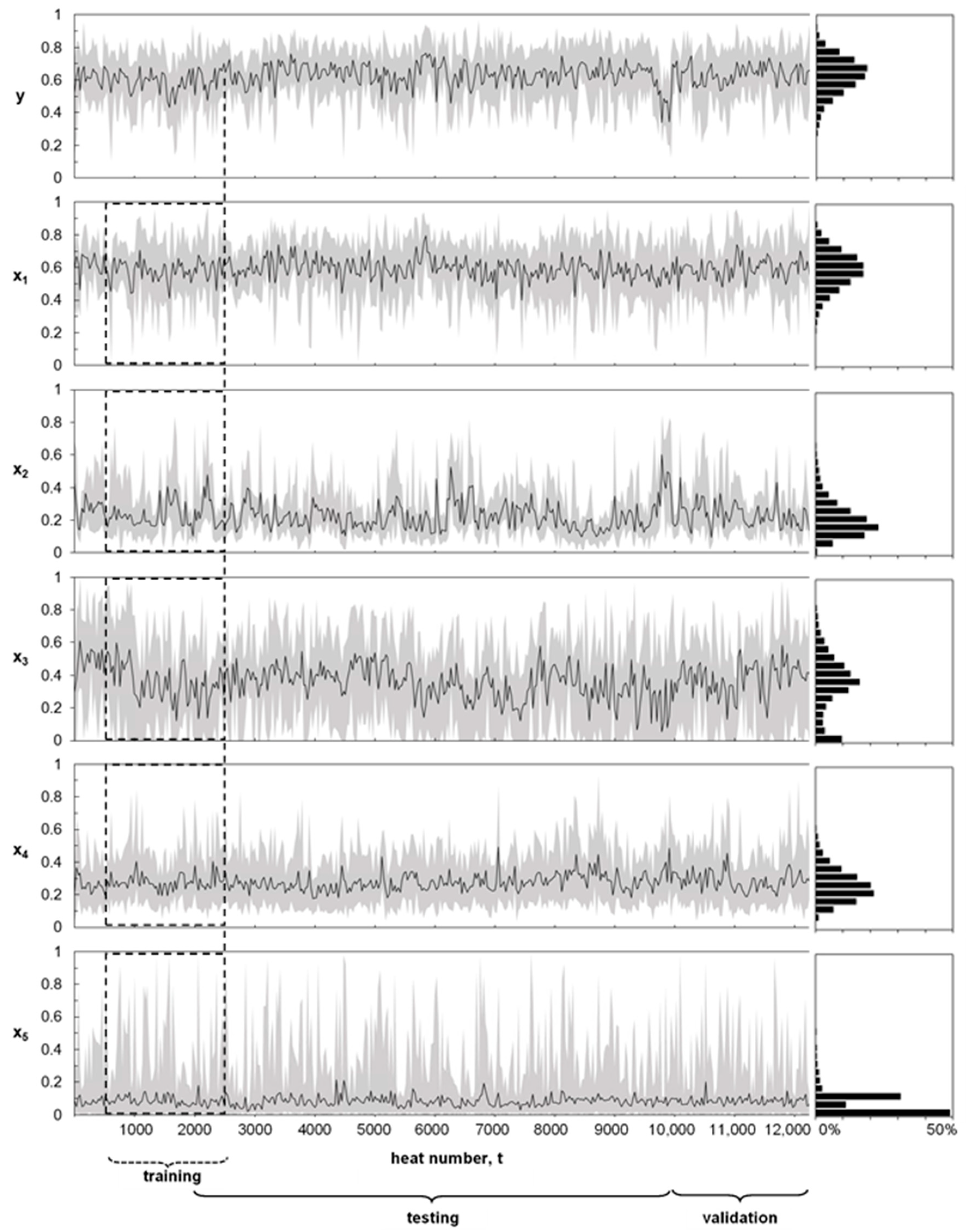
The normalized dataset is graphically displayed in Figure 2, where the minimum–maximum interval and the average value for groups of 30 heats are shown for clarity. This grouping size corresponds approximately to one production day.
It can be observed that initial and final temperatures x1 and y, respectively, exhibit similar distributions and temporal evolution. Rather than random changes, local tendencies can also be recognized; therefore, it seems appropriate to retain and exploit the time information contained in the data.
The similarities between y and x1 curves and histograms reflect the expected correlation between both variables. However, several features of the y curve do not match well with corresponding features of x1, as for example the drop in y that can be observed in the vicinity of t = 10,000. This indicates that other variables are also critical.
Total holding and empty vessels durations (x2, x4, and x5) have lower daily means, showing that normal production times are usually short with occasional longer times. Holding time x2 and empty torpedo time x4 are very similar, being dominated by torpedo logistics. Since empty torpedo movements are less critical than full ones, x4 has more dispersion than x2.
Empty ladle time, x4, exhibits a multimodal distribution showing the different process situations to which the steel plant reacts with a different number of hot metal ladles in service.
Daily average of pretreatment time x3, is much more centered as can be expected from prescribed desulfurization requirements. The bimodal histogram reveals that cases without pre-treatment (x3 = 0) are frequent.
2.3. Multivariate Adaptive Regression Splines with Moving Training Window
The application of multivariate adaptive regression splines (MARS) to hot metal temperature forecasting at BOF shop is investigated and its performance is assessed. The following model is proposed:
where the temperature prediction for heat number t, , is a function of the N selected explanatory variables for that heat t: . The model is constructed as a weighed sum of M basis functions, using constant weighing coefficients, . The w and t indexes in coefficients and functions indicate that, for every new prediction , both, basis functions and coefficients, are optimized by regression analysis using the w previous observations (, , … ). Hence, w represents the width of the moving training window.
The determination of coefficients in Equation (2) by regression analysis is straightforward, although there are multiple possible construction methods for the basis functions [41]. A non-parametric adaptive technique based on domain segmentation together with a simple sub-set of basis functions is adopted here. It was introduced in 1982 by Smith [42] for the univariate problem and extended for a multivariate setting in 1991 by Friedman [23,24] with the name of multivariate adaptive regression splines (MARS). A practical implementation of this technique, the ARESLAB toolbox for MATLAB, has been made publicly available by Jekabsons [32].
The model is built in two phases: Forward selection and backward deletion. In the forward pass, a pair of new basis functions is added at each step, resulting in an increasingly complex model that will not generalize well to new data. In the backward pass this overfitted model is pruned by removing the least effective term at each step.
2.3.1. Forward Phase
The forward phase starts with a model which consists of just the intercept term, that is, . At each additional step a new pair of basis functions is added to the model. Each new pair of basis functions consists of a basis function already existing in the model multiplied by a pair of functions of the form and , where the subscript “+” means the positive part, that is:
where xi is one of the input variables and c is one of the values of that input in the dataset (i.e., an observation of xi), which is usually referred to as the knot of the pair of basis functions. In other words, a new pair of functions from the collection
is multiplied by a basis function already in the model to obtain the new pair of basis functions. The algorithm compares all the combinations of existing terms, variables, and values for each variable in the data set.
One additional restriction is applied to the formation of basis functions: Each variable can appear at most once in a product (i.e., maximum self-interaction order, S = 1). This prevents the formation of higher-order powers of a single variable, which increase or decrease too sharply near the boundaries of the domain. Such powers can be approximated in a more stable way with piecewise linear functions. It is also possible to set an upper limit on the order of interaction between different variables, I. For example, a limit of two will allow pairwise products of linear functions, but not three or higher order products. An upper limit of one results in an additive model with no interactions between variables.
The coefficients βm are estimated by minimizing the residual sum-of-squares, that is, by standard linear regression finding the pair of basis functions that gives the maximum reduction in error. This pair is added to the model and this process of adding terms continues until the number of terms in the model reach a prescribed limit.
2.3.2. Backward Phase
At the end of the forward phase, a large model of the form in Equation (2) is obtained containing M = MF basis functions. This model typically overfits the data and will not generalize well to new data. Therefore, a backward deletion pass is applied by iteratively deleting the basis function whose removal causes the smallest increase in residual squared error until the model has only the intercept term. An estimated best model, for each model size λ, where λ is the number of terms in the model, is obtained at each step. Cross-validation could be used to estimate the optimal model size, but for computational savings the generalized cross-validation (GCV) is preferably used and works well in practice [23,43,44]:
The GCV criterion is the average-squared residual of the fit to the data, increased by a penalty factor that accounts for the increased variance associated with increasing model complexity C(λ) [32]:
where λ is the number of basis functions in the model including the intercept term, and d is the penalty. Since (λ − 1)/2 is the number of knots, C(λ) penalizes the model not only for its number of basis functions but also for its number of knots. Some mathematical and simulation results suggest that a price of three parameters for selecting a knot in a piecewise linear regression is a convenient choice (d = 3) for the general case, and two (d = 2) for an additive model [44]. However, d can always be selected as a model hyperparameter to be optimized.
The resulting GCV is an estimator of the mean squared error of the model in prediction mode, therefore the minimum value of GCV reflects a compromise between fit and model complexity, resulting in a better generalization of the model.
The forward pass adds basis functions in pairs at each step, while the backward pass deletes one basis function, the less relevant, at a time. Consequently, terms are often not seen in pairs in the final model.
In a previous modelling work, time series were applied to solve this problem. It was shown that the introduction of exogenous predictors into an auto-regressive integral moving average (ARIMA) model improved its performance [21]. Conversely, the potential benefit of introducing the L last observations of the predicted variable as input variables will be analyzed in the present work. Accordingly, for L > 0, in Equation (2) is expanded as .
2.3.3. Model Hyperparameters
As previously discussed, six possible model hyperparameters have been considered: S, I, MF, d, L, and w. The first four are typical settings of the standard MARS technique, while the last two (L and w) are the original of this study. In particular, w is a consequence of the novel continuous training approach adopted here which is required to ensure long-term performance of the model. The basic configuration of these six hyperparameters, together with the ranges to be tested, and the finally adopted configuration can be found in Table 2.
An initial hyperparameter set of {S = 1, I = 1, MF = 21, d = 2, L = 0, w = 1000} was taken as the base case. Self-interactions of variables where not allowed (S = 1) in order to avoid singularities near the boundaries of the domain [23,32]; this criterion was maintained along the study. The remaining parameters where varied to assess their effect on model performance. Interactions between variables where not allowed for the base case (I = 1) in order to start with a simple additive model. The maximum number of base functions in the forward phase, MF, was taken initially as maximum (21, 2N + 1), where N is the number of input variables, as suggested by Milborrow [45]. The GCV penalty per knot was chosen as d = 2, as suggested by Hastie [44] for additive models. Finally, the initial choices for w and L, were based on previous experiences of the authors [21,22].
3. Results
3.1. Computation
The proposed moving MARS model was implemented on MATLAB using the ARESLab toolbox [32]. The different cases were solved on a regular 64-bit laptop with a 2.6 GHz processor and 4 GB RAM. Computation cost was mainly due to the training of the model and it increased with the number of observations used to train de model, w, and the number of input variables, N = 5 + L. However, the resulting training time of a single case was always below 4 s. Considering that the interval between heats is typically 15–30 min, the computation time is far to be a limiting factor for the real time application of the model.
The model was developed using a test dataset formed by 10,000 registers. The initial 2000 registers were reserved for initializing the training window with a maximum of 2000 registers. Consequently, each study case involved testing 8000 different models, from t = 2000 to t = 10,000. The overall study required the evaluation of more than 2.4 × 10⁶ different models. Results were compared in terms of the mean absolute error (MAE). This is a convenient choice since the error of hot metal temperature forecast is proportional to the excess or defect in hot metal consumption [38]. Therefore, MAE reduction has a straight translation to economic savings and environmental improvements [36,37,38].
3.2. Study of Hyperparameters
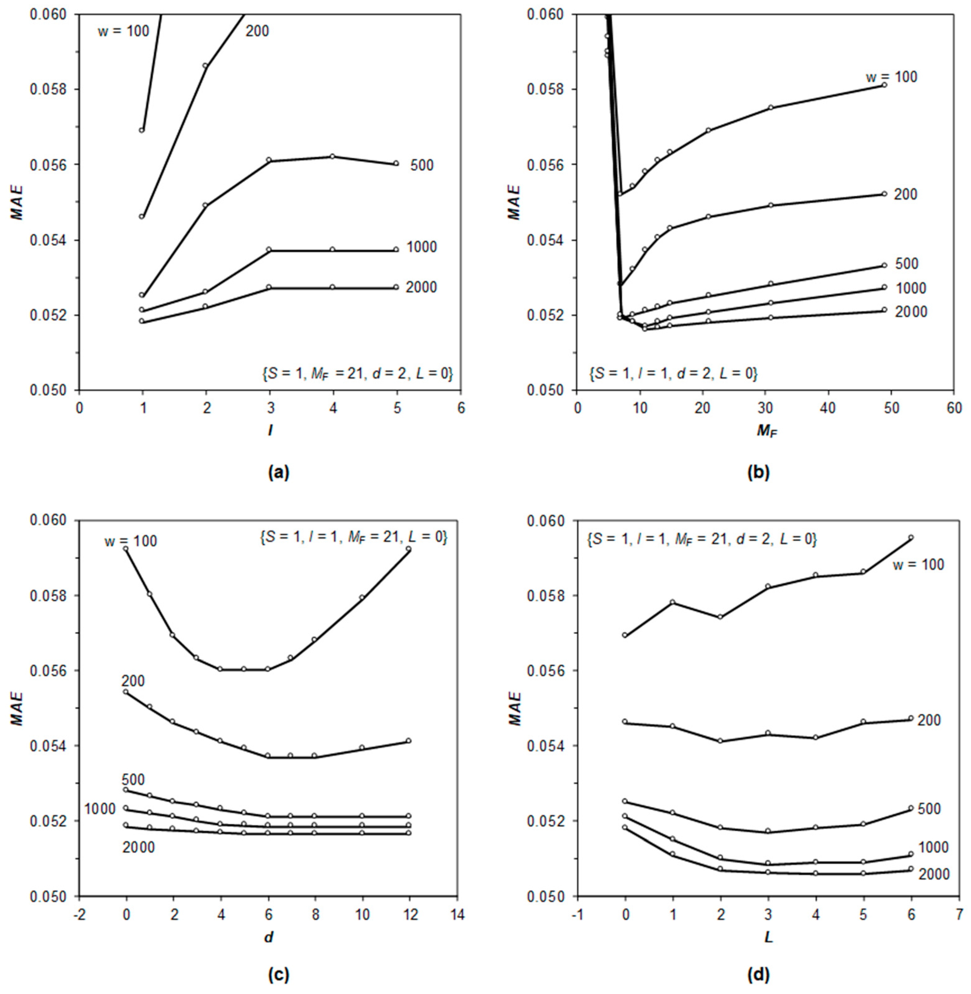
The influence of different parameter configurations on model performance is shown in Figure 3. It can be seen that w has a notable effect on model accuracy: The greater the w, the lower the MAE provided that the other hyperparameters are equal. This effect is more important for lower w; while for w > 1000 the reduction in MAE is lower than 0.0003. Additionally, the effect of any other hyperparameter tends to be lower as w increases. As a conclusion, it is interesting to set w ≥ 1000 not only to improve model accuracy but also to reduce its sensibility with regard to the other hyperparameters.
As shown in Figure 3a, if any order of interaction between input variables (I > 1) is allowed, the MAE increases. This effect is dramatic for w < 500 and much less pronounced for w > 500. This result suggests that the actual process performs in this way and that increasing I, only provides unnecessary degrees of freedom to the model, with the side effect of overfitting.
Figure 3b shows that the initial choice of MF = 21 for the maximum number of functions in the forward phase is close to its optimum value when w ≥ 1000. In fact, the best MAE for w = 1000 and 2000 is obtained when MF = 11 but the improvement in MAE is only around 0.0003 with regard to MF = 21. This finding suggests that, for this particular problem, MF = 2N + 1 is a good choice, but max(21, 2N + 1) = 21 can also be a reasonable selection for a large dataset [45]. The small effect of an additional increase of MF is logical, since the number of basis functions in excess at the end of the forward phase will be pruned in the backward phase of the method. However, MF still has some influence because GCV is a good proxy—but only a proxy—of the forecasting capabilities of the model. Consequently, increasing MF above the optimum gives slightly overfitted models.
The lowest MAE is obtained when the penalty for model complexity, d, is between 4 and 6 as can be seen in Figure 3c. For w < 500 a clear minimum is reached whereas for a larger w the MAE remains around the minimum for any d ≥ 6. Again, the effect in MAE is below 0.0004 for w ≥ 1000, indicating the robustness of generalization of the model when it is trained with enough data.
The introduction of the L previous observations of the predicted variable as additional predictors causes very different effects depending on the value of w. Figure 3d shows that for w = 100 it has an adverse effect on MAE, regardless the value of L. For w between 200 and 500 the improvement is modest (0.0003 to 0.0008), reaching a minimum for 2 < L < 4. Finally, for w ≥ 1000 an evident reduction of 0.0012 in MAE is attained for 3 < L < 5. This finding is in line with the results previously obtained for a simpler model based on moving average smoothing (MAS) [21]. In that case, in which the only predictors were the L previous observations of the predicted variable, the optimum value was 4 < L < 6. It can be inferred from both models that up to four or five previous observations give some information of the temperature tendency of the process. Older observations seem to be affected by changes in the process and they are not correlated with present conditions.
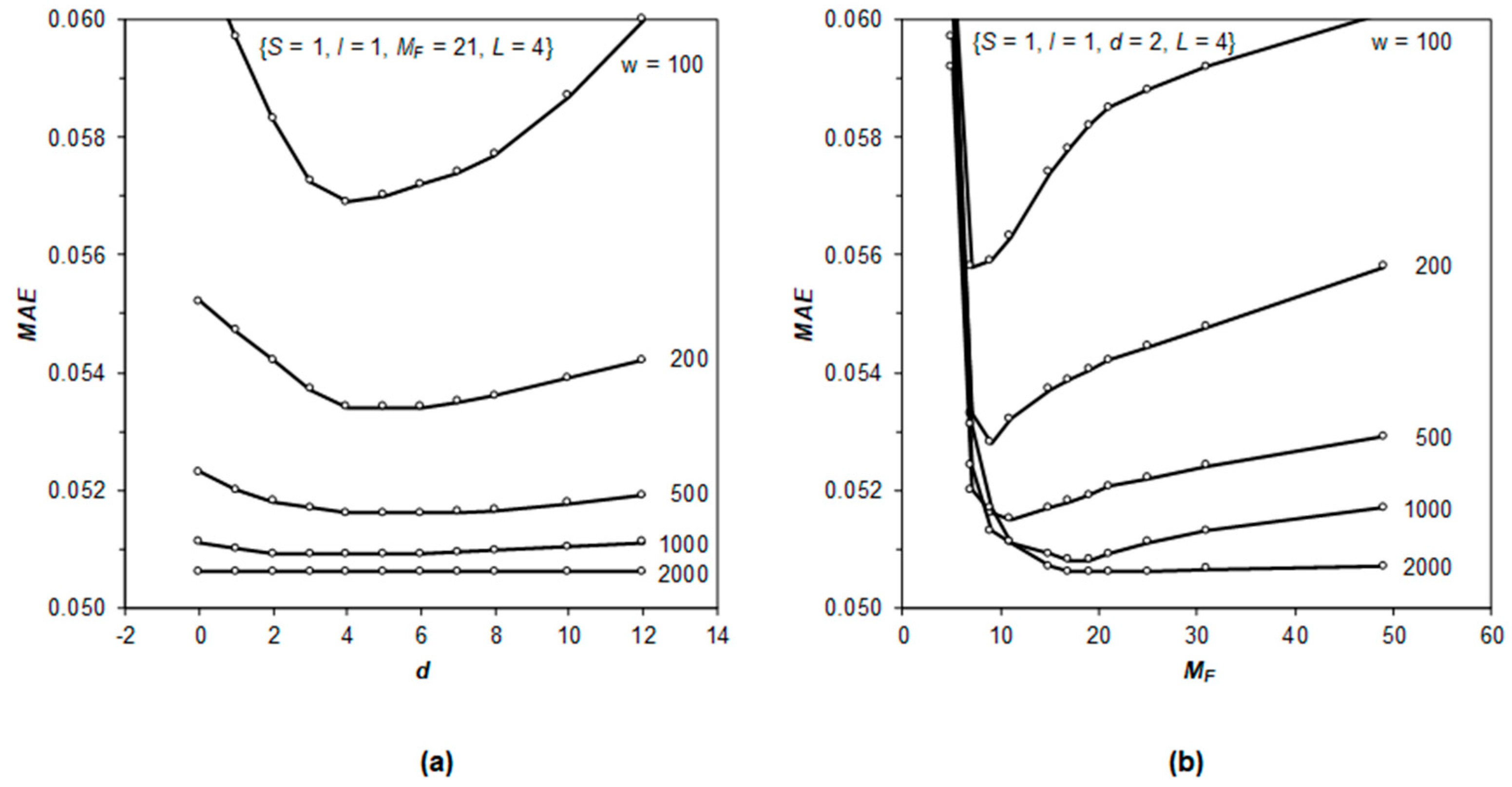
Finally, Figure 4 shows the effect of the most significant hyperparameters (MF, d, and w) when L = 4. It can be seen that the incorporation of four lagged observations not only improves MAE but also makes it less dependent on the other hyperparameters. For w = 2000, any MF > 15 gives the lowest MAE of 0.0506. Similarly, for w = 2000, any d ≥ 2 gives also the minimum MAE. It can be concluded that any model configuration within {S = 1, I = 1, MF > 15, d ≥ 2, L = 4, w = 2000} gives the best results.
3.3. Model Validation
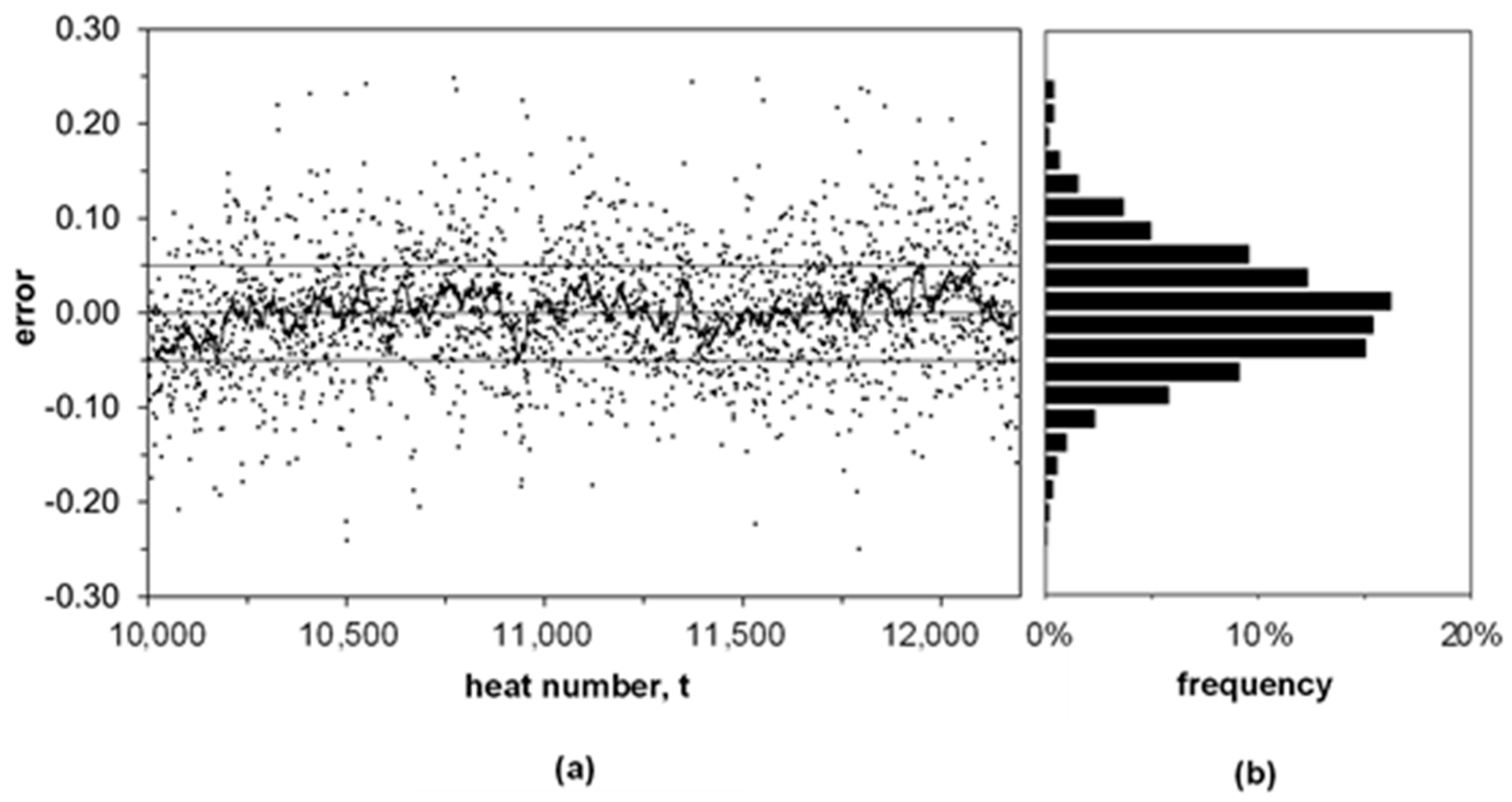
Based on the analysis described above, the final configuration of the model hyperparameters, indicated in Table 2, {S = 1, I = 1, MF = 21, d = 2, L = 4, w = 2000} was applied to the validation dataset for assessing the actual forecasting performance of the method. The model errors from t = 10,001 to t = 12,195 are shown in Figure 5.
The absolute errors are always lower than 0.25 and the daily mean error is always lower than 0.0500. The global MAE for the validation dataset is 0.05076 which is consistent with the value of 0.0506 obtained during hyperparameter optimization, confirming that GCV is a convenient estimator for the forecasting capability of the model [23,43,44].
4. Discussion
As indicated before, the application of the final MARS model {S = 1, I = 1, MF = 21, d = 2, L = 4, w = 2000} to the validation dataset provided 2195 evaluations of the method from t = 10,001 to t = 12,195. The resulting basis functions and coefficients in Equation (2) at t = 11,755 are shown in Table 3. The model at this point is taken as an example to discuss the features of the model. In this case, the model comprises 12 basis functions including the intercept term. Considering that 21 functions where allowed in the forward phase (MF = 21), it is inferred that nine functions with the lowest contribution to GCV where pruned in the backward phase.
As can be deducted from Table 3, the most important basis functions are those containing x1, x2, and x4, that is, the initial hot metal temperature, the total holding time, and the empty torpedo time, respectively. Empty ladle time and pre-treatment time have less importance; in fact, the actual temperature of the previous heat x6 = yt−1, is a better predictor. Moreover, the MARS method automatically excludes the less important variables. For this particular heat (t = 11,755), the actual temperature four heats before, x9 = yt−4, is not included in the model. This indicates that its contribution to model performance is negligible or even adverse. This is not the general case for every heat; for example, at t = 10,656 a basis function is also included for x9. In general, it is positive to include x9 in the model to improve its performance, as indicated in Figure 3c for curve w = 2000 at L = 4. It can be seen that some basis functions appear in pairs, as is the case for x1, x2, and x6. Other basis functions are individual, indicating that the corresponding symmetric functions were removed in the backward phase. A basis function without its symmetric variant indicates that either the involved variable is relevant only above a particular value (this is the case of x3, x5, x7, and x8), or in the lower part of its range (as for x4). As can be seen, the adaptive knot location of MARS method succeeds in capturing the nonlinearities of the data using segmented linear regression.
The model equations obtained for other heats have very similar shape with slight changes. The most important features are always present in the model. Other characteristics arise or go away depending on the history of the previous w heats.
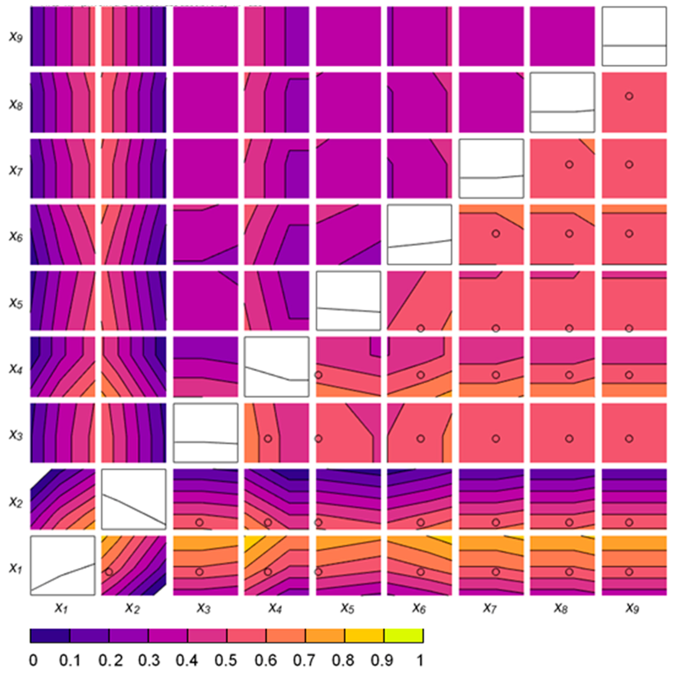
The actual shape of the basis functions can be better understood combining Table 3 and the graphical representation of the model in Figure 6. The line plots located in the diagonal of the mosaic show the model output, that is, the predicted hot metal temperature, , against each individual input variable, xi. The rest of the input variables are kept at their mid-points (xk = 0.5 for k ≠ i).
The line plot of versus x1 indicates that the effect of the initial temperature tends to damp as it increases. This is a coherent result, since higher thermal losses are foreseen from higher initial temperatures in all the phases of the process. A similar reasoning can be applied to the empty torpedo time, x4, considering that the thermal losses are expected to be higher for shorter times, since the lining temperature is higher. The effect of holding time, x2, and empty ladle time, x5, was found to be almost linear within the considered ranges, and with the anticipated slope, as can be seen in the related plots.
As predictable, the higher the temperature of the previous heats, the higher the expected temperature for the actual heat. Moreover, this effect seems to be only relevant, or more relevant, for higher temperatures. Although it can be hardly perceived in Figure 3 (but can be confirmed in Table 3), the slope of the line plot for versus x6 is smaller for x6 < 0.64. This behavior is more evident for x7 and x8 which are relevant only above 0.58 and 0.68, respectively.
The response surface for all the pair-wise combinations of the input variables are represented in the contour plots located above the diagonal in Figure 6. Again, the input variables outside the considered pair are kept at the mid-point of their ranges (xtk = 0.5 for k ≠ i and k ≠ j). It can be seen that the adaptive knot location succeeds in representing the non-linear features of the multivariate process dataset.
Finally, the response surface around the actual value of the input at heat number t = 11,755, is shown in the elements below the diagonal in Figure 6. Here, the color scale gives the predicted temperature ( = 0.056) and the circle marks the input vector.
The proposed model is dynamically trained for every new prediction to be made. This dynamic behavior is better appreciated in Figure S1, an animated version of Figure 6 showing model representation from t = 10,004 to t = 12,195. Figure S1 is included in the Supplementary Materials.
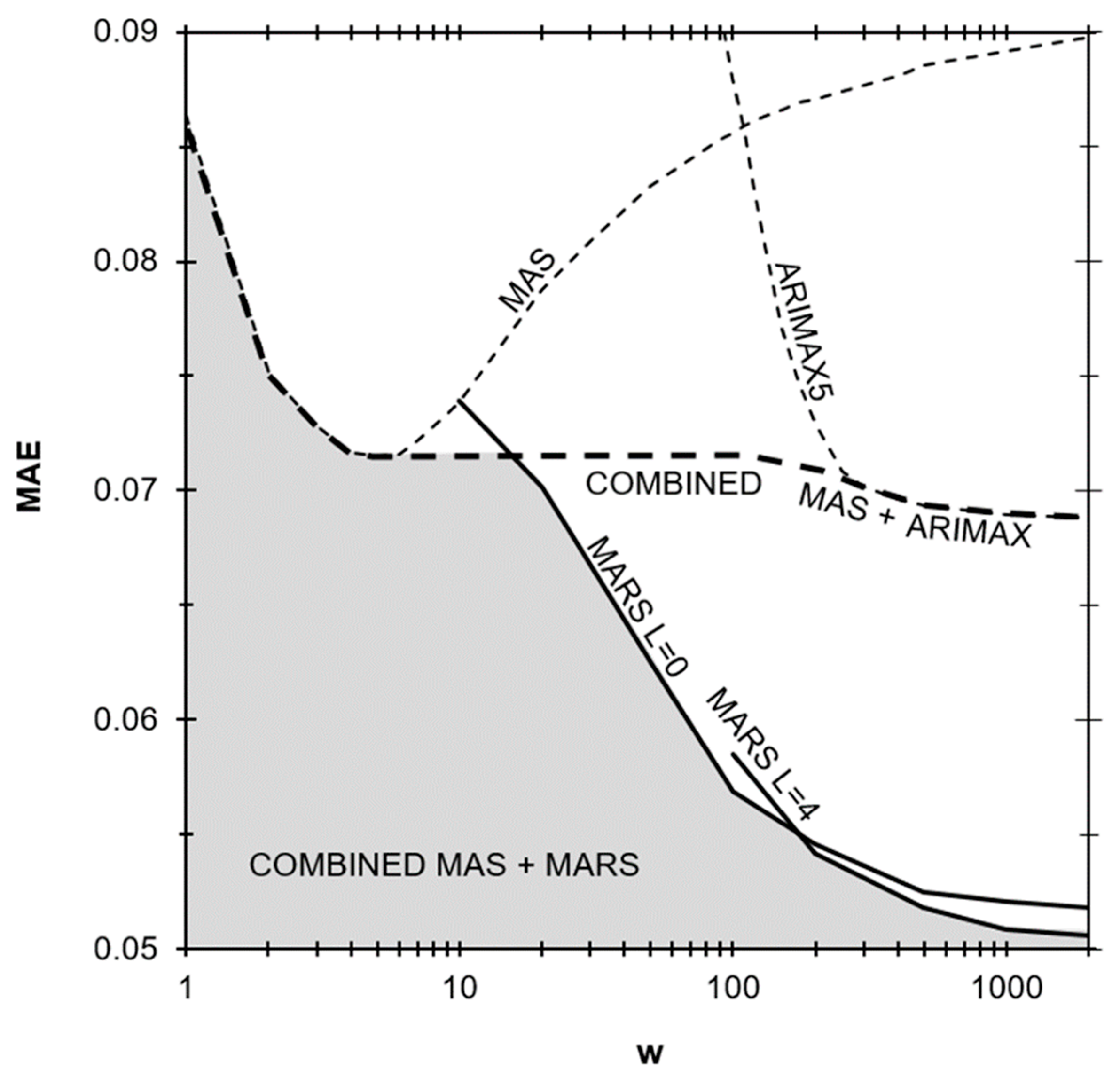
The good predictive performance of the proposed model can be better appreciated by comparison with other previously developed models as shown in Figure 7. A common reference model is the moving average smoothing (MAS) which forecasts temperature as the average of the w previous observations. The best MAE for this method is 0.0721 for w = 5; higher w values provide no benefit. However, for w > 100, time-series auto-regressive integral moving average with eXogenous predictors (ARIMAX) models can be applied providing a MAE below 0.0690 for w > 1000. On the other hand, for w > 20, any MARS configuration provides a major improvement over simple reference models but also over the more advanced ARIMAX models. The initial base configuration for MARS {S = 1, I = 1, MF = 21, d = 2, L = 0, w = 1000} gives a MAE of 0.0518 giving a 25% error reduction with reference to ARIMAX. The best performing MARS {S = 1, I = 1, MF = 21, d = 2, L = 4, w = 2000} provides 0.0506 of MAE, representing a 27% and a 30% of error reduction with regard to ARIMAX and MAS, respectively. This model configuration is the new benchmark for this problem.
As demonstrated in the previous section, the introduction of lagged terms as additional predictors further reduces the MAE of the model. However, it is worth noting that the higher the number of input variables, the higher the w required to obtain an optimum performance of the model, as can be seen in Figure 3d and Figure 7. The base configuration of MARS {S = 1, I = 1, MF = 21, d = 2, L = 0} requires at least ten previous observations of the five input variables, as illustrated in Figure 7. Configurations with additional input variables would require more than one hundred previous observations of all the inputs. This limitation poses a potential problem when some registers are missing in the process database. However, a judicious implementation of the model should relieve this problem, as indicated by the shaded region in Figure 7. This region delimits the lowest MAE that can be achieved by applying the best configuration for the available data-window at execution time.
5. Conclusions
An improved version of the standard MARS technique has been proposed for hot metal temperature forecasting at the steel plant. It employs five robust process variables and the four previous observations of the predicted variable as model inputs. A moving window approach is used for model training in order to avoid the need for periodic manual tuning.
There is no precedent for the application of MARS techniques to BOF steelmaking and a comparable temperature forecasting model of the BF–BOF interface has not been published before.
The effect of model hyperparameters in this problem has been explored and understood. The most influencing factor is the training window width, being the greater the best. However, widths above 1000 provided only marginal improvement in MAE. Similarly, the introduction of the four previous temperatures as additional predictions gave a small additional reduction in MAE. However, any little refinement in hot metal temperature forecasting is considered relevant, provided the mega-scale effect of the steelmaking industry [21,36,37,38].
The optimum hyperparameter configuration gave a MAE of 0.05076 (11.2 °C) on the validation phase. This result outperforms those of previous modelling attempts, with a MAE ranging from 0.083 to 0.069 (18.3 to 15.2 °C) [21].
The required computing time was lower than 4 s in total for training plus forecasting, the former thanks to GCV approximation, and the latter due to the simple mathematical formulation of the model. This computing time ensures real time operation, allowing reiterative execution for forecast updating.
The resulting model succeeds in capturing the non-linearities of the process but it is still easy to interpret. The model adapts to changes along time, since the relevant input variables, the number of basis functions and, of course, the fitting parameters are re-calculated for every new prediction. In a future work the adaptability performance of the model will be tested and optimized by introducing synthetic changes in the process.
Supplementary Materials
The following are available online at https://0-www-mdpi-com.brum.beds.ac.uk/2075-4701/10/1/41/s1, Video S1: MARS adaptability.
Author Contributions
Conceptualization, J.D. and F.J.F.; Methodology, J.D., F.J.F., and M.M.P.; Software, J.D. and F.J.F.; Validation, J.D. and F.J.F.; Formal analysis, J.D., F.J.F., and M.M.P.; Investigation, J.D.; Resources, J.D. and F.J.F.; Data curation, J.D.; Writing—original draft preparation, J.D. and F.J.F.; Writing—review and editing, J.D., F.J.F., and M.M.P.; Visualization, J.D.; Supervision, F.J.F.; Project administration, J.D. All authors have read and agreed to the published version of the manuscript.
Funding
This research received no external funding.
Acknowledgments
The authors would like to thank ArcelorMittal colleagues for their support and the valuable suggestions they provided. Their professional commitment has been the best stimulus for this contribution. The authors would like also to thank G. Jekabsons for creating and sharing the AresLab toolbox and A. González for supporting our initial ANN studies.
Conflicts of Interest
The authors declare no conflict of interest.
References
- McLean, A. The science and technology of steelmaking—Measurements, models, and manufacturing. Metall. Mater. Trans. B 2006, 37, 319–332. [Google Scholar] [CrossRef]
- Ghosh, A.; Chatterjee, A. Iron Making and Steelmaking: Theory and Practice; PHI Learning Pvt. Ltd.: New Delhi, India, 2008. [Google Scholar]
- Miller, T.W.; Jimenez, J.; Sharan, A.; Goldstein, D.A. Oxygen Steelmaking Processes. In The Making, Shaping, and Treating of Steel, 11th ed.; Fruehan, R.J., Ed.; The AISE Steel Foundation: Pittsburgh, PA, USA, 1998; pp. 475–524. [Google Scholar]
- Williams, R.V. Control of oxygen steelmaking. In Control and Analysis in Iron and Steelmaking, 1st ed.; Butterworth Scientific Ltd.: London, UK, 1983; pp. 147–176. [Google Scholar]
- Jiménez, J.; Mochón, J.; de Ayala, J.S.; Obeso, F. Blast furnace hot metal temperature prediction through neural networks-based models. ISIJ Int. 2004, 44, 573–580. [Google Scholar] [CrossRef]
- Martín, R.D.; Obeso, F.; Mochón, J.; Barea, R.; Jiménez, J. Hot metal temperature prediction in blast furnace using advanced model based on fuzzy logic tools. Ironmak. Steelmak. 2007, 34, 241–247. [Google Scholar] [CrossRef]
- Sugiura, M.; Shinotake, A.; Nakashima, M.; Omoto, N. Simultaneous Measurements of Temperature and Iron–Slag Ratio at Taphole of Blast Furnace. Int. J. Thermophys. 2014, 35, 1320–1329. [Google Scholar] [CrossRef]
- Jiang, Z.H.; Pan, D.; Gui, W.H.; Xie, Y.F.; Yang, C.H. Temperature measurement of molten iron in taphole of blast furnace combined temperature drop model with heat transfer model. Ironmak. Steelmak. 2018, 45, 230–238. [Google Scholar] [CrossRef]
- Pan, D.; Jiang, Z.; Chen, Z.; Gui, W.; Xie, Y.; Yang, C. Temperature Measurement Method for Blast Furnace Molten Iron Based on Infrared Thermography and Temperature Reduction Model. Sensors 2018, 18, 3792. [Google Scholar] [CrossRef] [Green Version]
- Pan, D.; Jiang, Z.; Chen, Z.; Gui, W.; Xie, Y.; Yang, C. Temperature Measurement and Compensation Method of Blast Furnace Molten Iron Based on Infrared Computer Vision. IEEE Trans. Instrum. Meas. 2018, 1–13. [Google Scholar] [CrossRef]
- Jin, S.; Harmuth, H.; Gruber, D.; Buhr, A.; Sinnema, S.; Rebouillat, L. Thermomechanical modelling of a torpedo car by considering working lining spalling. Ironmak. Steelmak. 2018, 1–5. [Google Scholar] [CrossRef]
- Frechette, M.; Chen, E. Thermal insulation of torpedo cars. In Proceedings of the Association for Iron and Steel Technology (Aistech) Conference Proceedings, Charlotte, NC, USA, 9–12 May 2005. [Google Scholar]
- Nabeshima, Y.; Taoka, K.; Yamada, S. Hot metal dephosphorization treatment in torpedo car. Kawasaki Steel Tech. Rep. 1991, 24, 25–31. [Google Scholar]
- Niedringhaus, J.C.; Blattner, J.L.; Engel, R. Armco’s Experimental 184 Mile Hot Metal Shipment. In Proceedings of the 47th Ironmaking Conference, Toronto, ON, Canada, 17–20 April 1988. [Google Scholar]
- Goldwaser, A.; Schutt, A. Optimal torpedo scheduling. J. Artif. Intell. Res. 2018, 63, 955–986. [Google Scholar] [CrossRef]
- Wang, G.; Tang, L. A column generation for locomotive scheduling problem in molten iron transportation. In Proceedings of the 2007 IEEE International Conference on Automation and Logistics, Jinan, China, 18–21 August 2007. [Google Scholar]
- He, F.; He, D.F.; Xu, A.J.; Wang, H.B.; Tian, N.Y. Hybrid model of molten steel temperature prediction based on ladle heat status and artificial neural network. J. Iron Steel Res. Int. 2014, 21, 181–190. [Google Scholar] [CrossRef]
- Du, T.; Cai, J.J.; Li, Y.J.; Wang, J.J. Analysis of Hot Metal Temperature Drop and Energy-Saving Mode on Techno-Interface of BF-BOF Route. Iron Steel 2008, 43, 83–86, 91. [Google Scholar]
- Liu, S.W.; Yu, J.K.; Yan, Z.G.; Liu, T. Factors and control methods of the heat loss of torpedo-ladle. J. Mater. Metall. 2010, 9, 159–163. [Google Scholar]
- Wu, M.; Zhang, Y.; Yang, S.; Xiang, S.; Liu, T.; Sun, G. Analysis of hot metal temperature drop in torpedo car. Iron Steel 2002, 37, 12–15. [Google Scholar]
- Díaz, J.; Fernández, F.J.; Suárez, I. Hot Metal Temperature Prediction at Basic-Lined Oxygen Furnace (BOF) Converter Using IR Thermometry and Forecasting Techniques. Energies 2019, 12, 3235. [Google Scholar] [CrossRef] [Green Version]
- Díaz, J.; Fernandez, F.J.; Gonzalez, A. Prediction of hot metal temperature in a BOF converter using an ANN. In Proceedings of the IRCSEEME 2018: International Research Conference on Sustainable Energy, Engineering, Materials and Environment, Mieres, Spain, 25–27 July 2018. [Google Scholar]
- Friedman, J.H. Multivariate adaptive regression splines. Ann. Stat. 1991, 19, 1–67. [Google Scholar] [CrossRef]
- Friedman, J.H.; Roosen, C.B. An Introduction to Multivariate Adaptive Regression Splines. Stat. Methods Med. Res. 1995, 4, 197–217. [Google Scholar] [CrossRef]
- Nieto, P.; Suárez, V.; Antón, J.; Bayón, R.; Blanco, J.; Fernández, A. A new predictive model of centerline segregation in continuous cast steel slabs by using multivariate adaptive regression splines approach. Materials 2015, 8, 3562–3583. [Google Scholar] [CrossRef] [Green Version]
- Mukhopadhyay, A.; Iqbal, A. Prediction of mechanical property of steel strips using multivariate adaptive regression splines. J. Appl. Stat. 2009, 36, 1–9. [Google Scholar] [CrossRef]
- Yu, W.H.; Yao, C.G.; Yi, X.D. A Predictive Model of Hot Rolling Flow Stress by Multivariate Adaptive Regression Spline. In Materials Science Forum; Trans Tech Publications Ltd.: Stafa-Zurich, Switzerland, 2017; Volume 898, pp. 1148–1155. [Google Scholar]
- Mehdizadeh, S.; Behmanesh, J.; Khalili, K. Comprehensive modeling of monthly mean soil temperature using multivariate adaptive regression splines and support vector machine. Theor. Appl. Climatol. 2018, 133, 911–924. [Google Scholar] [CrossRef]
- Yang, C.C.; Prasher, S.O.; Lacroix, R.; Kim, S.H. Application of multivariate adaptive regression splines (MARS) to simulate soil temperature. Trans. ASAE 2004, 47, 881. [Google Scholar] [CrossRef]
- Krzemień, A. Fire risk prevention in underground coal gasification (UCG) within active mines: Temperature forecast by means of MARS models. Energy 2019, 170, 777–790. [Google Scholar] [CrossRef]
- Kuhn, M.; Johnson, K. Nonlinear regression models. In Applied Predictive Modeling, 1st ed.; Springer: New York, NY, USA, 2010; pp. 145–151. [Google Scholar]
- Jekabsons, G. ARESLab: Adaptive Regression Splines Toolbox for Matlab/Octave. 2016. Available online: http://www.cs.rtu.lv/jekabsons/Files/ARESLab.pdf (accessed on 15 November 2019).
- Saltelli, A.; Ratto, M.; Andres, T.; Campolongo, F.; Cariboni, J.; Gatelli, D.; Tarantola, S. Global Sensitivity Analysis: The Primer; John Wiley & Sons: Chichester, UK, 2008. [Google Scholar]
- Mazumdar, D.; Evans, J.W. Elements of mathematical modeling. In Modeling of Steelmaking Processes, 1st ed.; CRC Press: Boca Raton, FL, USA, 2010; pp. 139–173. [Google Scholar]
- Sickert, G.; Schramm, L. Long-time experiences with implementation, tuning and maintenance of transferable BOF process models. Rev. Metall. 2007, 104, 120–127. [Google Scholar] [CrossRef]
- Ares, R.; Balante, W.; Donayo, R.; Gómez, A.; Perez, J. Getting more steel from less hot metal at Ternium Siderar steel plant. Rev. Metall. 2010, 107, 303–308. [Google Scholar] [CrossRef]
- Bradarić, T.D.; Slović, Z.M.; Raić, K.T. Recent experiences with improving steel-to-hot-metal ratio in BOF steelmaking. Metall. Mater. Eng. 2016, 22, 101–106. [Google Scholar] [CrossRef] [Green Version]
- Díaz, J.; Fernández, F.J. The impact of hot metal temperature on CO2 emissions from basic oxygen converter. Environ. Sci. Pollut. R. 2019, 1–10. [Google Scholar] [CrossRef]
- Geerdes, M.; Toxopeus, H.; van der Vliet, C. Casthouse Operation. In Modern Blast Furnace Ironmaking: An Introduction, 1st ed.; Verlag Stahleisen GmbH: Düsseldorf, Germany, 2015; pp. 97–103. [Google Scholar]
- Kozlov, V.; Malyshkin, B. Accuracy of measurement of liquid metal temperature using immersion thermocouples. Metallurgist 1969, 13, 354–356. [Google Scholar] [CrossRef]
- Jekabsons, G.; Zhang, Y. Adaptive basis function construction: An approach for adaptive building of sparse polynomial regression models. In Machine Learning, 1st ed.; IntechOpen Ltd.: London, UK, 2010; pp. 127–156. [Google Scholar]
- Smith, P.L. Curve Fitting and Modeling with Splines Using Statistical Variable Selection Techniques; Report NASA 166034; Langley Research Center: Hampton, VA, USA, 1982. [Google Scholar]
- Craven, P.; Wahba, G. Smoothing noisy data with spline functions. Numer. Math. 1978, 31, 377–403. [Google Scholar] [CrossRef]
- Hastie, T.; Tibshirani, R.; Friedman, J. MARS: Multivariate Adaptive Regression Splines. In The Elements of Statistical Learning: Data Mining, Inference and Prediction, 2nd ed.; Springer: New York, NY, USA, 2009; pp. 241–249. [Google Scholar]
- Milborrow, M.S. Package ‘Earth’. 9 November 2019. Available online: https://cran.r-project.org/web/packages/earth/earth.pdf (accessed on 18 January 2019).
Figure 1.
Hot metal process from blast furnace (BF) to basic-lined oxygen furnace (BOF) in which the following phases are considered: BF tapping, pre-treatment, transport, and transfer to BOF shop. To predict the final hot metal temperature, Y, five relevant variables are used as model inputs: Initial temperature X1, total elapsed time X2, pre-treatment duration X3, empty torpedo duration X4, empty ladle duration X5.

Figure 2.
Time evolution and histograms corresponding to the six involved variables. The dataset contains 12,195 registers covering one full production year. The first 10,000 heats were used for training and testing while the last 2195 were reserved for final validation. The minimum–maximum interval (gray area) and the average value (solid line) for groups of 30 heats are shown for clarity. The dashed boxes illustrate a moving training window of width w = 2000 for heat number t = 2500.

Figure 3.
Comparison of the mean absolute error (MAE) as a function of model hyperparameters: (a) Order of interaction between input variables, I; (b) maximum number of functions in the forward phase, MF; (c) penalty for model complexity, d; and (d) lagged terms as additional inputs, L. Each single point in a curve comprises 8000 evaluations of the model, from t = 2000 to t = 10,000.

Figure 4.
Effect of d, MF, and w on the mean absolute error (MAE) for L = 4: (a) Penalty for model complexity, d, and (b) maximum number of functions in the forward phase, MF. Each single point in a curve comprises 8000 evaluations of the model, from t = 2000 to t = 10,000.
Figure 4.
Effect of d, MF, and w on the mean absolute error (MAE) for L = 4: (a) Penalty for model complexity, d, and (b) maximum number of functions in the forward phase, MF. Each single point in a curve comprises 8000 evaluations of the model, from t = 2000 to t = 10,000.

Figure 5.
Prediction errors (with sign) of the final multivariate adaptive regression splines (MARS) model for the 2195 heats in the validation dataset: (a) Time evolution where each dot represents one heat and the solid curve represents the daily MAE (30 heat grouping) and (b) error distribution for individual heats.

Figure 6.
Graphical representation of the final MARS model {S = 1, I = 1, MF = 21, d = 2, L = 4, w = 2000} at heat number t = 11,755. The diagonal elements of the mosaic are the line plots of the predicted hot metal temperature, , versus each individual input variable, xi. The other mosaic elements are the response surfaces of the model for any combination of two variables (xi, xj); the contour plots below the diagonal are traced around the actual value of at t = 11,755: = (0.41, 0.14, 0.42, 0.38, 0.054, 0.53, 0.58, 0.61, 0.43) whereas the graphs above the diagonal are traced around the mid-point of the range of = (0.5, 0.5, 0.5, 0.5, 0.5) axes limits are [0,1] for all the variables.

Figure 7.
Comparison of the mean absolute error (MAE) as a function of the width of the training window, w. A single point in a curve comprises 8000 evaluations of the model, from t = 2001 to t = 10,000. The dashed bold line represents the best result obtained with a hybrid method based on moving average smoothing (MAS), and time series auto regressive integral moving average with exogenous predictors (ARIMAX). All methods were applied to the same dataset [21].


Table 1.
Model variables.
| Description | Symbol | Min | Max | Unit |
|---|---|---|---|---|
| Initial temperature | X1 | 1400 | 1540 | °C |
| Total holding time | X2 | 2 | 20 | h |
| Pre-treatment duration | X3 | 0 | 40 | min |
| Empty torpedo duration | X4 | 1 | 16 | h |
| Empty ladle duration | X5 | 0 | 8 | h |
| Final temperature | Y | 1200 | 1420 | °C |
Table 2.
Model hyperparameters with their initial values, explored ranges, and final configuration.
| Description | Symbol | Base | Min | Max | Final |
|---|---|---|---|---|---|
| Maximum self-interaction order | S | 1 | 1 | 1 | 1 |
| Maximum interaction order | I | 1 | 1 | 5 | 1 |
| Maximum functions in the forward phase | MF | 21 | 3 | 49 | 21 |
| Penalty for model complexity | d | 2 | 0 | 12 | 2 |
| Width of moving training window | w | 1000 | 10 | 2000 | 2000 |
| as additional predictors | L | 0 | 0 | 6 | 4 |
Table 3.
Model equations for MARS {S = 1, I = 1, MF = 21, d = 2, L = 4, w = 2000} at t = 11,755. The mean squared error (MSE) and the generalized cross validation (GCV) of the model predictions for the training data are 0.00408 and 0.00418, respectively. The columns MSE and GCV indicate the new values obtained when the basis function is removed from the model.
| Basis Function | Coefficient | MSE | GCV | ||
|---|---|---|---|---|---|
| 1 | 0.4411 | - | - | ||
| (x2 − 0.2672)+ | −0.5320 | 0.00541 | 0.00553 | ||
| (0.6998 − x4)+ | 0.3201 | 0.00526 | 0.00537 | ||
| (x1 − 0.4643)+ | 0.3777 | 0.00510 | 0.00521 | ||
| (0.2672 − x2)+ | 0.4428 | 0.00455 | 0.00465 | ||
| (0.4643 − x1)+ | −0.5489 | 0.00430 | 0.00439 | ||
| (0.6409 − x6)+ | −0.1124 | 0.00414 | 0.00423 | ||
| (x5 − 0.0312)+ | −0.0683 | 0.00412 | 0.00421 | ||
| (x6 − 0.6409)+ | 0.1408 | 0.00412 | 0.00421 | ||
| (x7 − 0.5818)+ | 0.0862 | 0.00411 | 0.00420 | ||
| (x3 − 0.4571)+ | −0.0526 | 0.00410 | 0.00419 | ||
| (x8 − 0.6818)+ | 0.0928 | 0.00409 | 0.00418 | ||
© 2019 by the authors. Licensee MDPI, Basel, Switzerland. This article is an open access article distributed under the terms and conditions of the Creative Commons Attribution (CC BY) license (http://creativecommons.org/licenses/by/4.0/).
Share and Cite
MDPI and ACS Style
Díaz, J.; Fernández, F.J.; Prieto, M.M. Hot Metal Temperature Forecasting at Steel Plant Using Multivariate Adaptive Regression Splines. Metals 2020, 10, 41. https://0-doi-org.brum.beds.ac.uk/10.3390/met10010041
AMA Style
Díaz J, Fernández FJ, Prieto MM. Hot Metal Temperature Forecasting at Steel Plant Using Multivariate Adaptive Regression Splines. Metals. 2020; 10(1):41. https://0-doi-org.brum.beds.ac.uk/10.3390/met10010041
Chicago/Turabian StyleDíaz, José, Francisco Javier Fernández, and María Manuela Prieto. 2020. "Hot Metal Temperature Forecasting at Steel Plant Using Multivariate Adaptive Regression Splines" Metals 10, no. 1: 41. https://0-doi-org.brum.beds.ac.uk/10.3390/met10010041
Note that from the first issue of 2016, this journal uses article numbers instead of page numbers. See further details here.