Prediction of the Bilinear Stress-Strain Curve of Aluminum Alloys Using Artificial Intelligence and Big Data

Abstract

Aluminum alloys are among the most widely used materials in demanding industries such as aerospace, automotive or food packaging and, therefore, it is essential to predict the behavior and properties of each component. Tools based on artificial intelligence can be used to face this complex problem. In this work, a computer-aided tool is developed to predict relevant mechanical properties of aluminum alloys—Young’s modulus, yield stress, ultimate tensile strength and elongation at break. These predictions are based on the alloy chemical composition and tempers, and are employed to estimate the bilinear approximation of the stress-strain curve, very useful as a decision tool that helps in the selection of materials. The system is based on the use of artificial neural networks supported by a big data collection about technological characteristics of thousands of commercial materials. Thus, the volume of data exceeds $5k$ entries. Once the relevant data have been retrieved, filtered and organized, an artificial neural network is defined and, after the training, the system is able to make predictions about the material properties with an average confidence greater than $95\%$. Finally, the trained network is employed to show how it can be used to support decisions about engineering applications.

1. Introduction

Aluminum alloys are some of the most relevant metallic materials of the industry and they play a very important role in some high-technology fields such as aerospace and in everyday industries such as food packaging [1], among other reasons, due to its high strength-to-weight ratio. Aluminum production and consumption has grown by approximately $50\%$ in the last decade and this rate is estimated to accelerate over the next few years [2,3]. In addition, it is expected to play a fundamental role at the ecological and environmental level because it is a relatively easy material to recycle [3].

Besides, aluminum alloys are the most frequent type of non-ferrous material employed for an extensive range of applications, namely in the automotive, aerospace, and structural industries, among others [4]. Widespread use of these alloys in the modern world is due to an exceptional blend of material properties, combining low density, excellent strength, corrosion resistance, toughness, electrical and thermal conductivity, recyclability and manufacturability. Another key factor is the relatively low cost of aluminum machining, making its alloys very attractive for applications in different sectors [4].

Aluminum was only discovered in the early 19th century, however, despite its short history, it has become an essential material. Every day, new uses for aluminum alloys are emerging in various industrial sectors due to its excellent properties [5] and the fact that the price of the raw material has been decreasing since then [2]. Therefore, it is necessary to provide material scientists with tools that can be used to develop new alloys with properties optimized for each need. The mechanical properties of a material play an important role in the performance of industrial components. A correct in-service behavior depends largely on the characteristics of the materials that constitute it, as inadequate material properties can cause premature failure [6,7]. Therefore, the decision to choose a specific material to manufacture an industrial component greatly affects its ability to carry out the work for which it was designed [8,9,10].

There are thousands of aluminum alloys although only a few of them are commonly used in the industry [11], in some cases due to the difficulty of finding new solutions and, in others, because they are specific materials with optimized characteristics for the mission they fulfill.

Knowing the properties of the materials employed in industrial designs is crucial; however, obtaining these data often involves accessing large amounts of resources, which are commonly not available. Multitude of tests are needed to obtain significant information, which entails that enough time, personnel and facilities must be available at a given cost [6]. The process of characterizing a material may involve a bulk of tests that requires a substantial amount of time and the investment of vast quantities of resources [12].

Despite the fact that there are multiple decision support systems and materials selection methodologies [13] applied to materials science, there are few references which mention the use of artificial intelligence-based technologies in the field of metal processing and engineering [6,14,15,16,17,18]. Although there are many studies that use machine learning to investigate the microstructure of metals and their properties [19,20,21], there are hardly any references with an industrial approach that take into account the tempers of aluminum alloys [22].

Nevertheless, it is possible to find a greater number of references that develop techniques based on artificial intelligence applied to other industrial materials, mainly steel [23]. These studies take advantage of the ability of these tools to obtain predictions about the behavior or properties of a certain material or industrial component [24,25,26,27,28].

In this work, a decision support system is developed which is capable of predicting some of the most important properties that define the stress-strain curve of aluminum alloys whose chemical composition and treatments (thermal and mechanical) are known. This system is capable of predicting the Young’s modulus (E), the yield stress ($YS$), the ultimate tensile strength ($UTS$) and the elongation at break (A). These four properties define the elastic and plastic behavior of a material under tension [29].

The difficulty of developing this study lies in the large number of steps and disciplines involved in carrying it out: an extensive software has been developed in Python 3.7 [30] capable of working without user intervention to download data from an on-line material library [31], filter and organize data, define and train an artificial neural network [32], and, finally, make predictions using that network. On the other hand, a great deal of work has been required to analyze data and define criteria based on materials science [33]. Developing the software to obtain and download the data to carry out this study has been one of the most delicate and time consuming steps.

1.1. Designation and Main Characteristics of Aluminum Alloys

Aluminum alloys are light materials with a high strength-to-weight ratio combined with excellent thermal conductivity and good corrosion resistance [5]. Aluminum has a density of about 2700 kg/m${}^3$, approximately one-third as much as steel (7830 kg/m${}^3$) [34]. Such lightweight, along with the high strength of some aluminum alloys (higher than some structural steels), allow designing and manufacturing of strong, lightweight structures that are particularly beneficial for vehicles [1,35] and for the environment.

Aluminum alloys are able to withstand the progressive oxidization that causes steel to rust away. The bare surface of aluminum reacts with oxygen to procedure an inert aluminum oxide film, that blocks further oxidation [35]. In addition, unlike iron rust, the aluminum oxide film does not flake off to expose a fresh surface that could be further oxidized. If that protective layer is scratched, it will immediately reseal itself. The thin oxide layer sticks tightly to the metal and is colorless and transparent [36,37].

Aluminum alloys and their tempers comprise a wide and adaptable assortment of manufacturing materials. For optimum product design and effective development, it is important to understand the differences between the available alloys, their performance and characteristics [34].

Aluminum is an example of a ductile material because it can withstand significant plastic deformation so they are very used in metal forming operations; such materials can be compressed to form thin plates and sheets or pulled to form wires [11]. Typical ductile materials show a stress-strain curve that is very steep at the beginning (elastic zone, where the stress-strain curve is almost a straight line) and, after the yield point, the curve slope decreases (plastic zone). At one point, the slope of the curve becomes zero at the ultimate tensile strength. The strain difference between the yield point and the ultimate point is relatively large for aluminum [38], due to their excellent ductility. Ductile materials have generally high toughness and are able to absorb a large amount of energy before breaking [12].

Appendix A contains a brief introduction to the nomenclature and standardization of aluminum alloys.

1.2. Modelization of Stress-Strain Curve

The stress-strain curve shows, in a simple way, the deformation of a material when it is subjected to mechanical load. In this diagram, the stress is plotted on y-axis and its corresponding strain on the x-axis [39]. Tension tests provide information on the strength and ductility of materials under uniaxial tensile stresses. This information may be useful in comparisons of materials, alloy development, quality control, numerical simulation such as finite element modeling, and design under certain circumstances [40].

The stress-strain curve is a crucial material asset and there are several standard testing methods to measure this curve, such as the tensile test [40], the compression test and the torsion test [38]. Although several studies have reported extension of the strain range [41], achieving a large strain with those methods sometimes can be difficult because the specimen tends to break at relative small strain points.

The simplest loading to visualize is a one-dimensional tensile test, in which a slender test specimen is stretched along its axis [42]. The stress-strain curve is a representation of the deformation of the specimen as the applied load is increased monotonically, usually to fracture [39]. Stress-strain curves are usually presented as:

• Engineering stress-strain curves, in which the initial dimensions of the specimens are used in the calculations.
• True stress-strain curves, where the instantaneous dimensions of the specimen at each point during the test are used in the calculations. The true curves are always above the engineering curves, notably in the higher strain portion of the curves [40].

A stress-strain curve combines a lot of information about the material and its behavior [43]. In this work, four of its properties will be studied:

• Young’s modulus (E)—it is a mechanical property that measures the stiffness of a material and characterizes its behavior in the elastic zone according to the Hooke’s law. It defines the ratio between uniaxial applied force and deformation of a material in the linear elastic regime (see Equation (1)) [44]:

  $$E=\frac{\sigma }{\epsilon },$$

  (1)

  where E is the Young’s modulus, $\sigma$ is the stress and $\epsilon$ is the strain.
• Yield strength ($YS$): it is a property of the material that indicates the point at which the material begins to deform plastically. Stresses lower than the $YS$ do not produce permanent deformations, whereas higher ones produce deformations that will remain even when the applied forces are eliminated [45].
• Ultimate tensile strength ($UTS$): the maximum stress that the material can withstand without area reduction [43].
• Elongation at break (A): the maximum strain that the material can withstand before failure [43].

These four properties completely define the bilinear approximation of the stress-strain curve of a material and allow summarizing the elasto-plastic stress behavior of a material to four values.

The stress-strain curve also indicates the amount of energy a material can store before fracture since the area enclosed below the curve is the energy that the material absorbs during its deformation [43,46]. The energy that a material absorbs is called resilience if the deformation is elastic and toughness if the deformation is plastic. This energy can be calculated using the Equation (2):

$$U=U_r+T={\int }_0^A\sigma ·d\epsilon ,$$

(2)

where U is the total deformation energy (absorbed energy), $U_r$ is the resilience, T is the toughness, A is the elongation at break, $\sigma$ is the stress and $\epsilon$ is the strain.

Since the transition from elastic to plastic behavior is continuous, for aluminum alloys (and for many other materials), there is no singular point that delimits them [47]. Therefore, standardization organizations have selected a criterion that guarantees the reproducibility of the tests—the yield point is defined as that in which there is a deviation of $0.2\%$ of strain with respect to the elastic linear behavior [48,49].

Figure 1 shows the true stress-strain curves of some relevant aluminum alloys. It is easy to distinguish the elastic regime (linear and very steep) and the plastic regime, where the curve slope decreases and becomes flatter. Thus, there is an obvious rapid change near the yield point.

To carry out some industrial design tasks, it is very common to use analytical models that allow the real curve of a material to be approximated using mathematical functions [51]. The behavior of aluminum alloys can be approximated very well by the expression of the Ramberg-Osgood stress-strain law [52] or by a bilinear stress-strain diagram, which is an accurate approximation away from the yield point [46,51,53,54,55].

The Ramberg-Osgood expression represents the elastoplastic behavior of the material throughout all its admissible strain values (see Equation (3)) [52,56].

$$\epsilon =\frac{\epsilon }{E}+\alpha \frac{\epsilon }{E}{\left(\frac{\sigma }{{\sigma }_{YS}}\right)}^{n-1},$$

(3)

where $\epsilon$ is the strain, $\sigma$ is the applied stress, E is the Young’s modulus, ${\sigma }_{YS}$ is the yield strength, and $\alpha$ and n are two parameters that depend on the material.

On the other hand, the bilinear approximation of the stress-strain curve consists of two lines that represent, respectively, the linear behavior (whose slope is the Young’s modulus, E) and the plastic behavior (whose slope is the strain hardening modulus, $E_T$) [43,56]. These two lines intersect at the yield point (see Equations (4) and (5)).

$$\epsilon =\frac{\sigma }{E},\sigma \le {\sigma }_{YS}$$

(4)

$$\epsilon =\frac{\sigma }{E_T},\sigma >{\sigma }_{YS},$$

(5)

where $\epsilon$ is the strain, $\sigma$ is the applied stress, E is the Young’s modulus, ${\sigma }_{YS}$ is the yield strength and $E_T$ is strain hardening modulus (the slope of the line that defines the plastic behavior).

Figure 2 shows a comparison between the actual stress-strain curve of a generic aluminum alloy and its bilinear approximation [55]. As can be seen, the fit of the simplified model is good away from the yield point, where the discrepancies are significant [56].

The shape of the stress-strain curve (real and approximate) and its values depend on [39]:

• Alloy chemical composition.
• Heat treatment and conditioning.
• Prior history of plastic deformation.
• The strain rate of the test.
• Temperature.
• Orientation of applied stress relative to the structure of the test specimens.
• Size and shape.

The latter four parameters are described in the pertinent standards, including the case of aluminum testing specimens [40,57]. The former three parameters are the ones that are considered in this study.

1.3. Sources of Big Data

Materials science depends on experiments and simulation-based models to understand the physics of materials in order to better know their characteristics and discover new materials with enhanced properties [58]. All these experiments and simulations generate a huge amount of data, which is becoming increasingly difficult to handle using traditional data processing techniques [6]. Due to the massive volume of data being produced at unprecedented speed, these data are not effectively processed to create information, delaying the production of new knowledge [59].

Traditionally, knowledge has been organized through the so-called “knowledge pyramid” or “information hierarchy”. This model is made up of four steps, each of which derives from the previous one—data, information, knowledge and wisdom (DIKW) [60]. In this way, the processed data constitutes information, which is organized to generate knowledge, which, finally, is summarized as wisdom [61].

Our current technology has reached a level never seen before in terms of generating data [58]; however, the techniques aimed at their processing are not yet as advanced and their use is not widespread [6]. Therefore, our society faces challenging problems to transform data into information and knowledge. Extracting value from raw data requires a systematic and well-defined approach to solve these emerging real-world problems and so, a new multidisciplinary approach is needed [59].

In any field, datasets are considered “big” when they are large, complex, and difficult to process and analyze. Materials science data tend to be particularly heterogeneous in terms of type and source. One of the first steps in processing large datasets is data reduction [62]. Experiments on the Large Hadron Collider, for example, retain only a small fraction of $1\%$ of the data they produce because it becomes impractical with the current technologies to store and analyze more than the hundreds of megabytes per second that are considered more valuable: it is up to sophisticated software to determine which data are more relevant [63].

Although the term “big data” is relatively new, the action of collecting and storing large amounts of information for further analysis has been performed for many years. The current definition of big data is based on the three Vs [6,64]:

• Volume: large volumes of unstructured low-density data are processed. The data can be of unknown value, such as machining conditions, material properties or manufacturing control measures.
• Velocity: the rate at which the data are received, and possibly, to which some action is applied.
• Variety: conventional data types are structured and can be clearly organized in a relational database; nevertheless, big data is presented as unstructured sparse registers.

Matmatch^® Munich, Germany [31] is a well-known open-access materials library that contains information about thousands of different commercial and standard materials. Registered users can freely access the information stored in the databases. A description sheet, which contains all available data, can be downloaded for each material [6].

Matmatch^® [31] offers widely sparse and heterogeneous data about more than 70,000 materials [65]. These data is provided by the manufacturers and suppliers of the materials. Although the data is believed to be accurate, it must be processed, filtered and parsed to generate a corpus of useful and meaningful information [61].

1.4. Artificial Intelligence and Artificial Neural Networks

Artificial intelligence (AI) is the simulation of human intelligence processes by machines, especially computer systems [66]. These processes comprise self-correction (spotting errors and solving them), reasoning (using rules to reach new conclusions and knowledge) and learning (acquiring procedures to employ the information) [6,67]. The term “artificial intelligence” was created in 1956 during the Dartmouth Conference, where the discipline arose [68]. At present, AI is a wide-ranging term that has lately gained importance due to the increase in speed, size and variety of the data collected by companies [67]. AI can perform tasks, such as recognizing patterns in data, more proficiently than humans do, which enables users to extract more information from their datasets [14].

AI is a term that encompasses a multitude of techniques and technologies aimed at endowing a machine with the ability to exhibit “intelligent behavior” [32]. Within these techniques, we can find simple (although powerful) mathematical models such as decision trees, capable of categorizing data [66]; and other much more complex and advanced technologies such as deep convolutional neural networks, able to identify images and patterns [69].

AI has shown that it can be applied to a multitude of disciplines not directly related to computing or robotics. Among the most relevant new uses, it can be highlighted medicine [70], warfare [71], ecology [72], security [73], education [74], oil exploration [75] or material science [76]. AI can be applied to almost all branches of science and engineering, and new uses and applications emerge every day [16,32].

Among all the tools included within the artificial intelligence field, multi-layer artificial neural networks (ANN) can be highlighted due to their current relevance and proven capabilities [77]. A multi-layer network is a supervised learning algorithm able to learn a non-linear function by training on a labelled dataset that can be used to perform classifications and regressions [78]. Multi-layer neural networks are made up of perceptrons that organize themselves forming layers (groups of neurons) that communicate with each other (in general, perceptrons do not communicate with their own layer companions) [6,17].

Bearing in mind the connection topology of the perceptrons, three types of layers can be defined: input layer, which includes all perceptrons that receive data from an external source; output layer, which includes all perceptrons that return results; and hidden layer, which includes all other perceptrons, which does not communicate with the network exterior [79].

Appendix B contains a mathematical explanation of the fundamentals of neural network technology.

2. Methodology

This work is focused on obtaining an artificial neural network capable of making acceptable predictions of the main parameters that define the stress-strain curve of aluminum alloys while maintaining a limited average error. Subsequently, the output data, the data about the network training process and the data about the prediction step are conveniently analyzed.

Figure 3 schematically shows an overview of the methodology of this work. It consists of two main phases: phase of dataset creation and phase of prediction and analysis. Each of these phases is made up of several stages that are based on the results of the previous one. This work scheme has already demonstrated its ability to obtain adequate results predicting material properties [6].

2.1. Stage A—Input Data Acquisition

As already indicated, the input dataset used in this work has been obtained from an online open access material library (Matmatch^® [31]). In this web portal, it is possible to access the information provided by thousands of suppliers of materials of different kinds, including aluminum alloys [6].

For each material, the registered data can be very diverse and, in any case, it should be noted that these data are not at all exhaustive, but quite sparse: not all information is available for all materials since the task of recording the data of each material depends on the marketers themselves. In the field of big data, it is very common to deal with sparse, heterogeneous and disperse information [64].

This material library offers information about more than 70,000 different materials [31]; including several thousand aluminum alloys registries. It is possible to access a specific datasheet for each material and download it; however, it is not possible to obtain a complete package with the information of multiple materials; instead, it is necessary to download the data of each material one by one [6].

To carry out the task of downloading the raw data of the relevant materials, a Python application has been developed which is capable of sequentially downloading the datasheets [30,80]. In this way, the raw data about 5341 aluminum alloys have been obtained. This bulk of registries contains data about 351 material properties, including chemical composition and mechanical, physical, electrical or acoustic properties. Each record is downloaded as an Excel document which contains all available information about the material; the datasheet format is not uniform neither the data is shown homogeneously [6].

2.2. Stage B—Data Organization and Filtering

Once the datasheets of all the materials have been downloaded, the information contained in all these files is sequentially read and interpreted. As already indicated, much more data is available than is necessary to carry out this study [31]. The following considerations have been taken when filtering and organizing the available data:

• The average value is taken for those properties that are registered as ranges in the datasheets. Some properties (especially chemical properties and some mechanical ones) are shown by specifying the maximum and minimum values because the standards and norms are written in this way [81,82].
• Only materials whose chemical composition is defined at more than $95\%$ are considered. For some alloys, the chemical composition is not specified or is poorly done [6].
• Only the four properties that define the bilinear approximation of the stress-strain curve are taken into account [39,56]: Young’s modulus (E), yield stress ($YS$), ultimate tensile strength ($UTS$) and elongation at break (A).
• Only records in which these four properties of the stress-strain curve are specified are considered [6]. Although the methodology is capable of inferring the missing information, it is necessary to know the real data in order to carry out the training or to calculate the precision of the prediction.
• Only eleven chemical elements (the main ones) are taken into account when defining the chemical composition of the alloys [35]: Al, Zn, Cu, Si, Fe, Mn, Mg, Ti Cr, Ni and Zr. All other chemical elements are considered non-relevant and their mass contribution is regrouped as “Other”. The presence of the discarded elements in the considered alloys is, in all cases, lower than $0.4\%$ (by mass) [81,82].
• The methodology only considers 35 different treatments: F (as fabricated, single type), O (annealed, single type), H (strain hardening, 19 types of treatment) and T (thermally treated, 14 types of treatments) [81,82]. Despite the fact that there are data about alloys with other treatments, it has been considered that the sample is so scarce that it causes bias [78] in the training process of the neural network and, so, these other treatments and their related registries have been discarded.

Approximately $84\%$ of discarded records are due to not indicating the four properties that define the bilinear stress-strain curve or because they do not specify any treatment. Note that an alloy whose manufacturing process does not involve treatments (therefore, F, as fabricated) is different from a material that does not specify any treatment (lack of data).

After conveniently filtering and organizing the 5341 datasheets, 2101 aluminum alloys records are kept. Only the following data are considered from now on:

• Young’s modulus (E), [GPa].
• Yield strength ($YS$), [MPa].
• Ultimate tensile strength ($UTS$), [MPa].
• Elongation at break (A), [mm/mm].
• Chemical composition (11 elements are considered), [% mass].
• Temper (35 treatments are considered).

2.3. Stage C—Artificial Neural Network Definition

Once the data has been filtered and has been guaranteed to be relevant, the artificial neural network that will be in charge of carrying out the predictions is defined: a multilayer feedforward architecture and a fully connected topology have been chosen [78]. This structure consists on one input layer, 3 hidden layers (which contain 100, 100 and 10 perceptrons respectively) and one output layer.

The multilayer feedforward architecture provides neural networks with the potential of being universal approximators [83]. Even though a fully connected ANN can represent any function, it may not be able to learn some functions because backpropagation convergence is not guaranteed [78].

This topology is the result of successive optimization steps to balance its learning capacity and the necessary resources for its training [84]. Note that a complex topology is capable of learning more complex functions than a simple topology but requires additional resources during its training: additional time, calculation capacity and input data [6]. A balance between the network depth and the network width was obtained.

2.4. Stage D—Artificial Neural Network Training and Prediction

Once the input data are already available and the neural network topology is defined, the training and prediction phase begins. During this phase, each of the four properties that define the bilinear approximation of the stress-strain curve is taken into account: Young’s modulus, yield strength, ultimate tensile strength and elongation at break.

For each of the four properties, 10 learning and prediction iterations are performed. Each of these iterations (independent from each other) is subdivided into four steps:

• Division of the input dataset: it is randomly divided into two disjoint subsets containing, respectively, $80\%$ (training subset) and $20\%$ (testing subset) of the records. To avoid bias, the same data should not be used to train and to make predictions since overfitting could occur and incorrect metrics (too good results) would be obtained [78].
• Neural network training with the training subset.
• Prediction of the properties of the test subset.
• Data storage for further analysis.

Figure 4 shows an overview of the iterative steps of the training and prediction phase. Repeating each iteration 10 times allows for a clearer view of the network performance metrics since better statistical analyzes can be carried out. The network training is subject to the following conditions:

• Calculation of the learning rate for each parameter using Adaptive Moment Estimation (ADAM) with ${\beta }_1=0.9$, ${\beta }_2=0.999$ (algorithm parameters), $\eta =0.001$ (step size) and $ϵ={10}^{-8}$ (stability factor) [85].
• Early stopping after 100 iterations without significant changes to avoid overfitting.
• Training stops when a training error of less than $0.001$ is reached as it is considered negligible [6].
• Maximum of $100,000$ training epochs to avoid infinite loops (this condition was never reached during this study).
• Sigmoid activation function.

This entire training and prediction process generates a large amount of information that provides very significant evidence about the performance and capabilities of the neural network.

2.5. Stage E—Output Analysis

Once all the training and prediction iterations have already been carried out and all the resulting information is available, the analysis phase is carried out. A complete battery of statistical metrics are calculated and several figures are plotted to summarize both the training and the prediction steps. This information allows the discussion of the results obtained with the methodology described in this paper.

The most remarkable information that can be obtained from the training is the evolution of the error function throughout the learning epochs. Although the number of epochs is not relevant, it is very important to check that the error function converges asymptotically to a relatively low value [78].

On the other hand, the performance of the prediction process is estimated using the absolute relative deviation for each sample of the test subsets. With this information, it is possible to calculate various statistical estimators and metrics that allow knowing the goodness and correctness of the complete methodology. In addition, it is possible to plot figures that represent this information.

Results out of $4.4$ sigma interval ($98\%$ confidence) are considered abnormal and are marked as outliers.

2.6. Software and Tools

The decision support system has been developed in Python 3.7 (Python Software Foundation: Beaverton, OR, USA) using an object-oriented paradigm [86] and the code architecture consists of more than 25 classes that interact and handle the different phases of the methodology. Multiple standard libraries and modules have been used to simplify the development, promote code reuse and take advantage of the latest technology [87]. Python has been chosen because it is a high-level, cross-platform, multi-paradigm programming language that is very popular among developers [30], especially those who develop artificial intelligence related software [88].

The most relevant external modules that have been used are:

• Selenium (version 3.141, Software Freedom Conservancy: New York, NY, USA): library that enables control of the web browser by using code [89].
• BeautifulSoup (v4.7.1, Free Software Foundation: Boston, MA, USA): library that facilitates working with HTML files and parsing them [90].
• SciPy (v1.2.3, Python Software Foundation: Beaverton, OR, USA): library that contains numerous scientific, mathematical and statistics functions [91].
• NumPy (v1.18.0, Python Software Foundation: Beaverton, OR, USA): library that enables easy management of large amounts of data and large matrices and numbers [91].
• MatPlot (v3.2.2, Python Software Foundation: Beaverton, OR, USA): library that eases the production of plots, figures and graphics [30].
• TensorFlow with Keras (v2.2, Google: Mountain View, CA, USA): high-level library that contains a vast amount of functions and procedures related to artificial intelligence, especially artificial neural networks [43,92].

The complete project includes more than 10,000 lines of code and works, mainly, on command line through batch processing. Only data analysis has really required active user intervention.

3. Results and Discussion

Even if the training algorithms are randomly initialized, the outcomes (during both training and prediction) are very stable and converge to similar results. Once the neural network is appropriately trained with the training subset, it is requested to make predictions. In this second step, the network is not given any clue about the expected results because this is the information that should be returned.

For each of the four properties, the network is trained with 1681 randomly chosen registers and the remaining 420 are employed to test the prediction performance of the network. Note that both subsets (training and testing) are randomly created for each of the 10 iterations; therefore, each iteration is fully independent from the others.

3.1. Young’S Modulus

Figure 5 shows the Young’s modulus histogram of the input dataset. It can be seen that the registers are grouped around the range $(69,71]$. This is an expected behavior since $E=70$ GPa is the most common value for aluminum alloys. It can also be seen that the range of values is quite small with very few records out of the range $(67,73]$.

Appendix C contains some notions about the neural network training process for predicting this property.

After the training, the neural network is asked to make predictions about the remaining records contained in the testing subset. For these records, the real values of the Young’s modulus are known but are not communicated to the ANN as they are retained to calculate some performance metrics afterwards.

The values contained in

Table 1. Average deviation (as %) of the prediction of the Young’s modulus.

Avg. Dev.	Std. Dev.	Median	Avg. Dev. 90%
3.07	2.24	2.35	2.87

are the relative errors of the prediction of the Young’s modulus (calculated using Equation (A8)). It shows several statistical indicators related to the deviation (as percentage) in the Young’s modulus prediction: average deviation (Avg. Dev.), statistical standard deviation (Std. Dev.), median and trimmed average deviation at 90% of the interval (Avg. Dev. 90%). The same information can be seen on Figure 6 as a box and whisker plot.

The overall average error is $3.07\%$, the median is $2.35\%$ and the trimmed average deviation at 90% is $2.87\%$. These three statistical values are quite close to each other, which means that the results are grouped around the mean value and few abnormal values appear.

Figure 6 shows the combined results of all 10 iterations. It is relevant to highlight the presence of some sparse outliers. These anomalous values are easily identifiable and, in general, are linked to very specific alloys that exhibit unusual properties. Although these outliers reduce the overall performance of the system, they allow knowing the capacity of the methodology in the worst conditions.

Figure 7 shows the histogram of the deviations in the Young’s modulus prediction for all iterations (it displays the 4200 predictions that are carried out in the 10 iterations). This plot shows that most of the errors are lower than $4\%$, however, some high values appear for alloys with unusual properties. The neural network has trouble learning the properties of these alloys because the sample in the input dataset is small and they diverge with respect to the behavior of the other alloys (this issue would be solved with a more complete input dataset).

Since the overall average deviation is $3.07\%$, it can be said that the system makes very low errors when predicting the value of the Young’s modulus. Furthermore, the median and the trimmed average are very close to the average, so it can be confirmed that hardly any bad results appear.

3.2. Yield Strength

Figure 8 shows the histogram of the yield strength values of the input dataset. These data are quite disperse and do not exhibit any predominant value. The yield strength strongly depends on the chemical composition of the alloy and the treatment applied to it. For instance, Al 7075-O (no treatment) alloy has a $YS=140$ MPa, while Al 7075-T6 (heat treatment) shows a $YS=455$ MPa [93]. As shown in Figure 8, the yield strength of aluminum alloys is a property that exhibits a wide range of values.

As already indicated, the position of the yield point is based on conventions (usually a deviation of $0.2\%$ from the linear behavior) since, in fact, no significant physical phenomenon occurs in it [48]. Therefore, it is a property for which there is usually considerable uncertainty even in the reference bibliography (this data is usually given in the form of a range of values) [93].

Appendix C contains some notions about the neural network training process for predicting this property.

Once the training has been successfully completed, the neural network is asked to make predictions about the data from the testing subset. The averaged statistical metrics of

Table 2. Average deviation (as %) of the prediction of the yield strength.

Avg. Dev.	Std. Dev.	Median	Avg. Dev. 90%
4.58	3.40	3.78	4.33

are obtained after performing the 10 training-prediction iterations.

Table 2 shows the averaged information regarding the relative errors (according to Equation (A8)) of the 10 iterations: relative average deviation (Avg. Dev.), statistical standard deviation (Std. Dev.), median and trimmed average deviation at 90% (Avg. Dev. 90%).

The average precision of the prediction (average relative error) is $4.58\%$ with a standard deviation of $3.40\%$. It is noteworthy that the average deviation, the median and the trimmed average deviation at 90% show very similar values ($4.58\%$, $3.78\%$ and $4.33\%$ respectively), which indicates that the results are concentrated and few anomalous values appear. Figure 9 shows this same information in the form of a box and whisker diagram. In addition, this figure shows the outliers that have appeared during the process.

Figure 10 shows the histogram of the deviations of the yield strength prediction for all iterations (it shows the 4200 predictions that are made in the 10 iterations). This plot shows that most of the errors are lower than $6\%$. The error of the yield strength estimation is low (average $4.58\%$) but the results are more dispersed than in the case of Young’s modulus because, as already indicated, it is a property that has an inherent uncertainty.

3.3. Ultimate Tensile Strength

Figure 11 shows the histogram of the ultimate tensile strength values for all records in the input dataset. These data are heterogeneously distributed over a very wide range of values and, although a maximum appears in the range $(175,205]$, it cannot be considered as truly remarkable. This figure highlights the great diversity of values that this property takes.

Appendix C contains some notions about the neural network training process for predicting this property.

Table 3. Average deviation (as %) of the prediction of the ultimate tensile strength

Avg. Dev.	Std. Dev.	Median	Avg. Dev. 90%
3.30	2.82	2.55	3.08

shows various averaged statistical metrics about the relative error of the predictions (see Equation (A8)) that have been carried out: average deviation (Avg. Dev.), statistical standard deviation (Std. Dev.), median and trimmed average deviation at 90% (Avg. Dev. 90%). The average relative error of the system is $3.30\%$, being $2.55\%$ and $3.08\%$ the median and the trimmed average deviation at 90% respectively. These very low values account for the performance of the methodology.

Figure 12 shows the result of the averaged prediction precision in the form of a box and whisker diagram. The presence of some abnormal values that have been marked as outliers should be highlighted. In this case, those anomalous results are related to alloys that exhibit unusually low ultimate tensile strength values and for which there are few samples in the input dataset.

Figure 13 shows a histogram of the errors made by the system throughout the 10 iterations that have been carried out. It is remarkable that there are few results greater than $6\%$ and, in any case, most of the values are included in the range $[0,3)$.

The system is more performant predicting the ultimate tensile strength than the yield strength because the former has a physical meaning and, therefore, the data in the input dataset is more precise.

3.4. Elongation at Break

Figure 14 shows the histogram of elongation at break for the entire input dataset. In this case, the data exhibits a wide range of values although they are concentrated around low values. Aluminum alloys, in general, are more ductile than steel and therefore easier to work with [34].

Elongation at break is a very difficult property to determine since it requires an exhaustive test campaign that involves working with very high deformations, which implies very low straining rates [50]. Moreover, the behavior of the testing probes greatly depends on the metallurgic microstructure, the exact chemical composition and the treatments [34,50]. Therefore, the available data for this property is not very precise and is usually shown in the form of ranges, for example, the elongation at break of the Al 7075-T6 is 5–$11\%$ [39,93].

Appendix C contains some notions about the neural network training process for predicting this property.

Table 4. Average deviation (as %) of the prediction of the elongation at break.

Avg. Dev.	Std. Dev.	Median	Avg. Dev. 90%
5.90	4.05	5.33	5.73

shows various statistical metrics related to the performance of the predictions. In the table, each column contains, respectively, the average deviation (Avg. Dev.), the statistical standard deviation (Std. Dev.), the median and the trimmed average deviation at 90% (Avg. Dev. 90%).

These results show a lower predictive performance than in the case of the other three considered properties: the mean deviations are higher ($5.90\%$, $5.33\%$ and $5.73\%$ for the average, the median and the trimmed average). It is also noteworthy that the statistical standard deviation (Std. Dev.) is also greater ($4.05\%$), which indicates that the results of these predictions are more scattered.

Figure 15 shows the averaged result of the predictive performance of the 10 iterations in the form of a box and whisker diagram. The results are more dispersed than in the other three cases and a few outliers with very high values appear. The network has been trained with data that, by its own nature, are imprecise (ranges) and it causes the results to be more heterogeneous. Figure 16 shows the histogram of the relative errors obtained in the prediction of the elongation at break for all the iterations. This plot shows that the deviations are concentrated on low values, with few abnormally high results.

3.5. Limitations of the Methodology

The main limitation of this study is the size of the input dataset and the ability of the neural network to learn from it [32]. As already indicated, the outcomes of this methodology improve when the training process is carried out using a larger input set. However, obtaining large amounts of material data is difficult because it consumes a huge amount of resources (time, money, people...). Therefore, a larger initial information corpus can improve the results.

As previously described, the topology model that has been employed in this study has some disadvantages (e.g., the results are affected by a limited initial dataset and the local minimums generate substantial attraction) that constitute a drawback of the procedure [6]. Other neural networks architectures can improve the results or reduce the required resources to carry out the training phase.

This study is founded on the assumption that the data obtained from the material library are correct and reliable [31]. The correctness of the input data do not modify the methodology but it can affect the results because the neural network would learn incorrect information.

4. Example of Application

The Al 2024-T4 alloy has been selected to develop this example because there is extensive information about it, it is easily comparable with data from leading sources and it is a widely used industrial material. Al 2024-T4 is a copper-based aluminum alloy (Al 2xxx) that has been treated with the T4 temper (solution heat-treated and natural aged) [81]. It has the highest ductility compared to the other variants of 2024 aluminum [1].

This is one of the best-known aluminum alloys due to its high strength and excellent fatigue behavior; it is widely used in structures and parts where a good strength-to-weight ratio is required [34]. Al 2024 alloy is easily machined to a high quality surface finish; moreover, it is easily plastically formed in the annealed condition (Al 2024-O) and, then, can be heat-treated to become Al 2024-T4. Since its resistance to corrosion is relatively low, this aluminum is commonly used with some type of coating or surface treatment [37].

Table 5. Al 2024-T4 chemical composition [81].

Element	Weight %
Al	90.7–94.7
Cr	Max. 0.1
Cu	3.8–4.9
Fe	Max. 0.5
Mg	1.2–1.8
Mn	0.3–0.9
Other	Max. 0.15
Si	Max. 0.5
Ti	Max. 0.15
Zn	Max 0.25

shows the chemical composition of Al 2024-T4 and

Table 6. Actual mechanical properties of the Al 2024-T4 [93].

Property	Value
Young’s modulus [GPa]	73
Yield strength [MPa]	395
Ultimate tensile strength [MPa]	470
Elongation at break [%]	19

shows the mechanical properties that are relevant to this study [93].

Before launching the software that carries out the training and prediction, to avoid overfitting, all references to Al 2024-T4 and -T351 (this is an identical standard regarding mechanical properties [93]) have been removed from the input dataset. In the same way as previously explained, 10 training-prediction iterations have been executed.

Table 7. Properties prediction for Al 2024-T4.

Property	Actual val.	Avg. val.	Std. Dev.	Median	Max.	Min.
E [GPa]	73	73.3	0.7	73.4	74.3	71.9
$YS$ [MPa]	395	395.1	9.3	395.9	409.4	376.5
$UTS$ [MPa]	470	471.5	8.0	470.8	483.2	460.1
A [%]	19	19.0	0.8	18.9	20.1	17.7

shows the actual values (Actual val.) and the results of the prediction of the mechanical properties of Al 2024-T4, as well as some other statistical metrics that allow quantifying the error and the performance of the methodology for this particular case: average predicted value (Avg. val.), statistical standard deviation of the predictions (Std. Dev.), median, maximum (Max.) and minimum (Min.).

Table 8. Prediction error for Al 2024-T4 (as %).

Property	Avg. error	Std. Dev.	Median	Max.	Min.
E [%]	0.84	0.55	0.81	1.77	0.08
$YS$ [%]	1.63	1.62	0.95	4.68	0.20
$UTS$ [%]	1.35	0.98	1.44	2.81	0.13
A [%]	3.21	2.34	3.08	6.89	0.05

shows various statistical results that summarize the predictive error for this alloy (the results are shown as a percentage). Note that the average errors do not exceed, in any case, $3.5\%$. The same information can be seen in Figure 17. With this information, it can be assured that the results adjust very well to the actual values.

Note that the distribution of average errors is consistent with what was said previously: the better predictive performances have been obtained for the Young’s modulus and the ultimate tensile strength, and the worse results for the yield strength and the elongation at break. This is also true for the statistical standard deviation values.

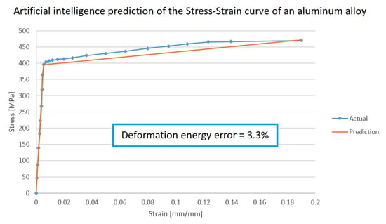
Figure 18 shows the actual stress-strain curve for Al 2024-T6 [50] and its bilinear approximation using the average values resulting from the prediction using the methodology described in this work (see Table 7). Note that the predicted curve fits the actual one (especially in the elastic region); however, discrepancies appear near the yield point and in the plastic zone.

The discrepancy between the two curves can be quantified by calculating the difference in deformation energies (see Equation (2)) [43,46]. This is equivalent to calculating the area enclosed between both curves. The deformation energy difference between the two curves is $2.74$ MJ, so, $3.3\%$ of the actual energy ($83.8$ MJ). This deviation is also an indication of the error made when using the approximation instead of the real curve.

Keeping the methodology error below $5\%$ implies a similar performance as the typical artificial intelligence-based methodologies applied to materials science [24,25]. On the other hand, a similar error rate would be comparable, according to the Lean Manufacturing framework, to that of an industrial system working at a four-sigma level, which has traditionally been associated with the average industry in developed countries [94,95].

As already indicated, obtaining the stress-strain curve of a material is a slow, expensive and resource-intensive process. However, based on this example, it can be said that using the methodology described in this paper allows shortening deadlines and having an estimate of the expected results.

5. Conclusions and Future Work

This article has investigated the feasibility of using artificial neural networks and big data to predict the stress-strain curve of aluminum alloys whose chemical composition and previous treatments are known. The possibilities of artificial intelligence techniques have been explored based on large datasets. Therefore, the main conclusions of this work are presented as follows:

• Artificial neural network technology can be employed to exploit large material datasets to predict the mechanical properties of aluminum alloys. An ANN can learn to estimate the value of a material property based on its chemical composition and temper.
• An artificial neural network can be trained to predict the bilinear approximation of the stress-strain curve of an aluminum alloy if its chemical composition and tempers are well defined. The prediction error remains limited and the average deviations in this work for the Young’s module, the yield strength, the ultimate tensile strength and the elongation at break are, respectively, $3.07\%$, $4.58\%$, $3.30\%$ and $5.90\%$.
• Supervised learning methodologies require large training datasets to achieve satisfactory predictive performance. The predictive ability of a neural network improves as the dataset grows because it has more samples to learn from, and therefore, the network can approximate better the reality of the problem.
• A multilayer artificial neural network can be trained to approximate nonlinear functions related to materials science. Theoretically, a multilayer neural network can learn to approximate any nonlinear function if the training dataset is large enough and if it has a sufficient number of perceptrons [83].

This work contributes to applying innovative techniques such as those based in artificial intelligent techniques in materials science and technology research as it provides a new development tool to consider new aluminum alloys. It allows obtaining a first approximation and, therefore, focusing resources on the most promising materials. In addition, it opens the door to investigate similar solutions applied to other metals.

Artificial neural networks have proven to be a suitable ally to describe the elastoplastic behavior of highly relevant industrial materials without the need of expensive and complicated stress-strain tests. It can be studied whether it is possible to design a system based on artificial intelligence capable of predicting the stress-strain curve more accurately or using other better approaches such as the Ramberg-Osgood one [52].

Other more performant network architectures can be explored since this work scheme has shown that it is possible to use them to make these predictions. There is a wide spectrum of network topologies that cover different needs [78], which suggests that other solutions can be investigated.

References

1. Danylenko, M. Aluminium alloys in aerospace. Alum. Int. Today 2018, 31, 35. [Google Scholar]
2. Galevsky, G.; Rudneva, V.; Aleksandrov, V. Current State of the World and Domestic Aluminium Production and Consumption; IOP Conference Series: Materials Science and Engineering; IOP Publishing: Novokuznetsk, Russia, 2018; Volume 411, p. 012017. [Google Scholar]
3. Soo, V.K.; Peeters, J.; Paraskevas, D.; Compston, P.; Doolan, M.; Duflou, J.R. Sustainable aluminium recycling of end-of-life products: A joining techniques perspective. J. Clean. Prod. 2018, 178, 119–132. [Google Scholar] [CrossRef] [Green Version]
4. Branco, R.; Berto, F.; Kotousov, A. Mechanical Behaviour of Aluminium Alloys; MDPI Applied Sciences: Basel, Switzerland, 2018. [Google Scholar]
5. Ashkenazi, D. How aluminum changed the world: A metallurgical revolution through technological and cultural perspectives. Technol. Forecast. Soc. Chang. 2019, 143, 101–113. [Google Scholar] [CrossRef]
6. Merayo, D.; Rodríguez-Prieto, A.; Camacho, A. Prediction of Physical and Mechanical Properties for Metallic Materials Selection Using Big Data and Artificial Neural Networks. IEEE Access 2020, 8, 13444–13456. [Google Scholar] [CrossRef]
7. Morini, A.A.; Ribeiro, M.J.; Hotza, D. Early-stage materials selection based on embodied energy and carbon footprint. Mater. Des. 2019, 178, 107861. [Google Scholar] [CrossRef]
8. Piselli, A.; Baxter, W.; Simonato, M.; Del Curto, B.; Aurisicchio, M. Development and evaluation of a methodology to integrate technical and sensorial properties in materials selection. Mater. Des. 2018, 153, 259–272. [Google Scholar] [CrossRef] [Green Version]
9. Mousavi-Nasab, S.H.; Sotoudeh-Anvari, A. A comprehensive MCDM-based approach using TOPSIS, COPRAS and DEA as an auxiliary tool for material selection problems. Mater. Des. 2017, 121, 237–253. [Google Scholar] [CrossRef]
10. Das, D.; Bhattacharya, S.; Sarkar, B. Decision-based design-driven material selection: A normative-prescriptive approach for simultaneous selection of material and geometric variables in gear design. Mater. Des. 2016, 92, 787–793. [Google Scholar] [CrossRef]
11. Alam, T.; Ansari, A.H. Review on Aluminium and its alloys for automotive applications. Int. J. Adv. Technol. Eng. Sci. 2017, 5, 278–294. [Google Scholar]
12. Kamaya, M.; Kawakubo, M. A procedure for determining the true stress–strain curve over a large range of strains using digital image correlation and finite element analysis. Mech. Mater. 2011, 43, 243–253. [Google Scholar] [CrossRef]
13. Rodríguez-Prieto, Á.; Camacho, A.M.; Sebastián, M.Á. Materials selection criteria for nuclear power applications: A decision algorithm. JOM 2016, 68, 496–506. [Google Scholar] [CrossRef]
14. Dimiduk, D.M.; Holm, E.A.; Niezgoda, S.R. Perspectives on the impact of machine learning, deep learning, and artificial intelligence on materials, processes, and structures engineering. Integr. Mater. Manuf. Innov. 2018, 7, 157–172. [Google Scholar] [CrossRef] [Green Version]
15. Liu, Y.; Zhao, T.; Ju, W.; Shi, S. Materials discovery and design using machine learning. J. Mater. 2017, 3, 159–177. [Google Scholar] [CrossRef]
16. Wang, Y.; Wu, X.; Li, X.; Xie, Z.; Liu, R.; Liu, W.; Zhang, Y.; Xu, Y.; Liu, C. Prediction and Analysis of Tensile Properties of Austenitic Stainless Steel Using Artificial Neural Network. Metals 2020, 10, 234. [Google Scholar] [CrossRef] [Green Version]
17. Javaheri, E.; Kumala, V.; Javaheri, A.; Rawassizadeh, R.; Lubritz, J.; Graf, B.; Rethmeier, M. Quantifying Mechanical Properties of Automotive Steels with Deep Learning Based Computer Vision Algorithms. Metals 2020, 10, 163. [Google Scholar] [CrossRef] [Green Version]
18. Abbas, A.T.; Pimenov, D.Y.; Erdakov, I.N.; Taha, M.A.; El Rayes, M.M.; Soliman, M.S. Artificial intelligence monitoring of hardening methods and cutting conditions and their effects on surface roughness, performance, and finish turning costs of solid-state recycled Aluminum alloy 6061 chips. Metals 2018, 8, 394. [Google Scholar] [CrossRef] [Green Version]
19. Zhou, T.; Song, Z.; Sundmacher, K. Big Data Creates New Opportunities for Materials Research: A Review on Methods and Applications of Machine Learning for Materials Design. Engineering 2019, 5, 1017–1026. [Google Scholar] [CrossRef]
20. Schmidt, J.; Marques, M.R.; Botti, S.; Marques, M.A. Recent advances and applications of machine learning in solid-state materials science. Npj Comput. Mater. 2019, 5, 1–36. [Google Scholar] [CrossRef]
21. Ly, H.B.; Le, L.M.; Duong, H.T.; Nguyen, T.C.; Pham, T.A.; Le, T.T.; Le, V.M.; Nguyen-Ngoc, L.; Pham, B.T. Hybrid artificial intelligence approaches for predicting critical buckling load of structural members under compression considering the influence of initial geometric imperfections. Appl. Sci. 2019, 9, 2258. [Google Scholar] [CrossRef] [Green Version]
22. Ling, J.; Antono, E.; Bajaj, S.; Paradiso, S.; Hutchinson, M.; Meredig, B.; Gibbons, B.M. Machine Learning for Alloy Composition and Process Optimization. In Proceedings of the ASME Turbo Expo 2018: Turbomachinery Technical Conference and Exposition, Oslo, Norway, 11–15 June 2018; American Society of Mechanical Engineers Digital Collection: New York, NY, USA, 2018. [Google Scholar]
23. Twardowski, P.; Wiciak-Pikuła, M. Prediction of Tool Wear Using Artificial Neural Networks during Turning of Hardened Steel. Materials 2019, 12, 3091. [Google Scholar] [CrossRef] [Green Version]
24. Asteris, P.G.; Roussis, P.C.; Douvika, M.G. Feed-forward neural network prediction of the mechanical properties of sandcrete materials. Sensors 2017, 17, 1344. [Google Scholar] [CrossRef] [PubMed] [Green Version]
25. De Filippis, L.A.C.; Serio, L.M.; Facchini, F.; Mummolo, G.; Ludovico, A.D. Prediction of the vickers microhardness and ultimate tensile strength of AA5754 H111 friction stir welding butt joints using artificial neural network. Materials 2016, 9, 915. [Google Scholar] [CrossRef] [PubMed] [Green Version]
26. Moayedi, H.; Kalantar, B.; Abdullahi, M.M.; Rashid, A.S.A.; Nazir, R.; Nguyen, H. Determination of Young Elasticity Modulus in Bored Piles Through the Global Strain Extensometer Sensors and Real-Time Monitoring Data. Appl. Sci. 2019, 9, 3060. [Google Scholar] [CrossRef] [Green Version]
27. Sun, D.; Lonbani, M.; Askarian, B.; Armaghani, D.J.; Tarinejad, R.; Pham, B.T.; Huynh, V.V. Investigating the Applications of Machine Learning Techniques to Predict the Rock Brittleness Index. Appl. Sci. 2020, 10, 1691. [Google Scholar] [CrossRef] [Green Version]
28. Abambres, M.; Rajana, K.; Tsavdaridis, K.D.; Ribeiro, T.P. Neural Network-based formula for the buckling load prediction of I-section cellular steel beams. Computers 2019, 8, 2. [Google Scholar] [CrossRef] [Green Version]
29. Szumigała, M.; Polus, Ł. An numerical simulation of an aluminium-concrete beam. Procedia Eng. 2017, 172, 1086–1092. [Google Scholar]
30. Lutz, M. Programming Python: Powerful Object-Oriented Programming; O’Reilly Media, Inc.: Newton, MA, USA, 2010. [Google Scholar]
31. GmbH, Matmatch Matmatch. Available online: https://matmatch.com/ (accessed on 15 April 2020).
32. Jackson, P.C. Introduction to Artificial Intelligence; Courier Dover Publications: Mineola, NY, USA, 2019. [Google Scholar]
33. Callister, W.D.; Rethwisch, D.G. Materials Science and Engineering; John Wiley & Sons: New York, NY, USA, 2011; Volume 5. [Google Scholar]
34. Kaufman, J.G. Introduction to Aluminum Alloys and Tempers; ASM International: Almere, The Netherlands, 2000. [Google Scholar]
35. Davis, J.R. Alloying: Understanding the Basics; ASM International: Almere, The Netherlands, 2001. [Google Scholar]
36. Scamans, G.; Butler, E. In situ observations of crystalline oxide formation during aluminum and aluminum alloy oxidation. Metall. Trans. A 1975, 6, 2055–2063. [Google Scholar] [CrossRef]
37. Gui, F. Novel corrosion schemes for the aerospace industry. In Corrosion Control in the Aerospace Industry; Elsevier: Amsterdam, The Netherlands, 2009; pp. 248–265. [Google Scholar]
38. Yogo, Y.; Sawamura, M.; Iwata, N.; Yukawa, N. Stress-strain curve measurements of aluminum alloy and carbon steel by unconstrained-type high-pressure torsion testing. Mater. Des. 2017, 122, 226–235. [Google Scholar] [CrossRef]
39. ASM. Atlas of Stress-Strain Curves; ASM: Almere, The Netherlands, 2002. [Google Scholar]
40. ASTM, E8–99. Standard Test Methods for Tension Testing of Metallic Materials (ASTM E8/E8M–16AE1); ASTM: West Conshohocken, PA, USA, 2001. [Google Scholar]
41. Bacha, A.; Maurice, C.; Klocker, H.; Driver, J.H. The large strain flow stress behaviour of aluminium alloys as measured by channel-die compression (20-500 C). Mater. Sci. Forum 2006, 519, 783–788. [Google Scholar] [CrossRef]
42. Huang, C.; Jia, X.; Zhang, Z. A modified back propagation artificial neural network model based on genetic algorithm to predict the flow behavior of 5754 aluminum alloy. Materials 2018, 11, 855. [Google Scholar] [CrossRef] [PubMed] [Green Version]
43. Nageim, H.; Durka, F.; Morgan, W.; Williams, D. Structural Mechanics–Loads, Analysis. In Materials and Design of Structural Elements, 7th ed.; Pearson International: England, UK, 2010. [Google Scholar]
44. ASTM, Committee E-28 on Mechanical Testing. Standard Test Method for Young’s Modulus, Tangent Modulus, and Chord Modulus; ASTM International: West Conshohocken, PA, USA, 2004. [Google Scholar]
45. Hahn, G.; Rosenfield, A. Metallurgical factors affecting fracture toughness of aluminum alloys. Metall. Trans. A 1975, 6, 653–668. [Google Scholar] [CrossRef]
46. Fertis, D.G. Infrastructure Systems: Mechanics, Design, and Analysis of Components; John Wiley & Sons: Hoboken, NJ, USA, 1997; Volume 3. [Google Scholar]
47. Christensen, R.M. Observations on the definition of yield stress. Acta Mech. 2008, 196, 239–244. [Google Scholar] [CrossRef]
48. Christensen, R.M. The Theory of Materials Failure; Oxford University Press: Oxford, UK, 2013. [Google Scholar]
49. Johnson, G.; Holmquist, T. Test Data and Computational Strength and Fracture Model Constants for 23 Materials Subjected to Large Strains, High Strain Rates, and High Temperatures; Los Alamos National Laboratory, LA-11463-MS: Los Alamos, NM, USA, 1989; Volume 198.
50. Nicholas, T. Material behavior at high strain rates. Impact Dyn. 1982, 1, 277–332. [Google Scholar]
51. Gere, J.; Goodno, B. Deflections of Beams. In Mechanics of Materials, 8th ed.; Cengage Learning: Boston, MA, USA, 2012. [Google Scholar]
52. Ramberg, W.; Osgood, W.R. Description of Stress-Strain Curves by Three Parameters; NASA: Washington, DC, USA, 1943.
53. Rasmussen, K.J.; Rondal, J. Strength curves for metal columns. J. Struct. Eng. 1997, 123, 721–728. [Google Scholar] [CrossRef]
54. Pelletier, H.; Krier, J.; Cornet, A.; Mille, P. Limits of using bilinear stress–strain curve for finite element modeling of nanoindentation response on bulk materials. Thin Solid Films 2000, 379, 147–155. [Google Scholar] [CrossRef]
55. Eurocode 9—Design of Aluminium Structures; BSI: London, UK, 2007.
56. Mazzolani, F. EN1999 Eurocode 9— Design of aluminium structures. In Proceedings of the Institution of Civil Engineers-Civil Engineering; Thomas Telford Ltd.: London, UK, 2001; Volume 144, pp. 61–64. [Google Scholar]
57. ISO-EN. 6892-1. Metallic Materials-Tensile Testing—Part 1: Method of Test at Room Temperature; International Organization for Standardization: Geneva, Switzerland, 2009.
58. Agrawal, A.; Choudhary, A. Perspective: Materials informatics and big data: Realization of the “fourth paradigm” of science in materials science. APL Mater. 2016, 4, 053208. [Google Scholar] [CrossRef] [Green Version]
59. Song, I.Y.; Zhu, Y. Big data and data science: What should we teach? Expert Syst. 2016, 33, 364–373. [Google Scholar] [CrossRef]
60. Rowley, J. The wisdom hierarchy: Representations of the DIKW hierarchy. J. Inf. Sci. 2007, 33, 163–180. [Google Scholar] [CrossRef] [Green Version]
61. Batra, S. Big data analytics and its reflections on DIKW hierarchy. Rev. Manag. 2014, 4, 5. [Google Scholar]
62. White, A.A. Big data are shaping the future of materials science. MRS Bull. 2013, 38, 594–595. [Google Scholar] [CrossRef] [Green Version]
63. García-Gil, D.; Ramírez-Gallego, S.; García, S.; Herrera, F. Principal components analysis random discretization ensemble for big data. Knowl. Based Syst. 2018, 150, 166–174. [Google Scholar] [CrossRef]
64. Erl, T.; Khattak, W.; Buhler, P. Big Data Fundamentals: Concepts, Drivers & Techniques; Prentice Hall Press: Upper Saddle River, NJ, USA, 2016. [Google Scholar]
65. Weinbub, J.; Wastl, M.; Rupp, K.; Rudolf, F.; Selberherr, S. ViennaMaterials–A dedicated material library for computational science and engineering. Appl. Math. Comput. 2015, 267, 282–293. [Google Scholar] [CrossRef]
66. Merayo, D.; Rodriguez-Prieto, A.; Camacho, A. Comparative analysis of artificial intelligence techniques for material selection applied to manufacturing in Industry 4.0. Procedia Manuf. 2019, 41, 42–49. [Google Scholar] [CrossRef]
67. Helal, S. The expanding frontier of artificial intelligence. Computer 2018, 51, 14–17. [Google Scholar] [CrossRef]
68. McCarthy, J.; Minsky, M.L.; Rochester, N.; Shannon, C.E. A proposal for the dartmouth summer research project on artificial intelligence, August 31, 1955. AI Mag. 2006, 27, 12. [Google Scholar]
69. Krizhevsky, A.; Sutskever, I.; Hinton, G.E. Imagenet classification with deep convolutional neural networks. In Proceedings of the Advances in Neural Information Processing Systems, Lake Tahoe, NV, USA, 3–6 December 2012; pp. 1097–1105. [Google Scholar]
70. Johnson, K.W.; Soto, J.T.; Glicksberg, B.S.; Shameer, K.; Miotto, R.; Ali, M.; Ashley, E.; Dudley, J.T. Artificial intelligence in cardiology. J. Am. Coll. Cardiol. 2018, 71, 2668–2679. [Google Scholar] [CrossRef]
71. Cummings, M. Artificial Intelligence and the Future of Warfare; Chatham House for the Royal Institute of International Affairs London: London, UK, 2017. [Google Scholar]
72. Villa, F.; Ceroni, M.; Bagstad, K.; Johnson, G.; Krivov, S. ARIES (Artificial Intelligence for Ecosystem Services): A new tool for ecosystem services assessment, planning, and valuation. In Proceedings of the 11th Annual BIOECON Conference on Economic Instruments to Enhance the Conservation and Sustainable Use of Biodiversity, Venice, Italy, 21–22 September 2009; pp. 21–22. [Google Scholar]
73. Allen, G.; Chan, T. Artificial Intelligence and National Security; Belfer Center for Science and International Affairs: Cambridge, MA, USA, 2017. [Google Scholar]
74. Ee, J.H.; Huh, N. A study on the relationship between artificial intelligence and change in mathematics education. Commun. Math. Educ. 2018, 32, 23–36. [Google Scholar]
75. Kolesov, V. Cognitive Modelling in Oil & Gas Exploration and Reservoir Prediction. In Proceedings of the 80th EAGE Conference and Exhibition 2018, Copenhaga, Dinamarca, 11–14 November 2018; European Association of Geoscientists & Engineers: Houten, The Netherlands, 2018; Volume 2018, pp. 1–5. [Google Scholar]
76. Thankachan, T.; Prakash, K.S.; Pleass, C.D.; Rammasamy, D.; Prabakaran, B.; Jothi, S. Artificial neural network to predict the degraded mechanical properties of metallic materials due to the presence of hydrogen. Int. J. Hydrog. Energy 2017, 42, 28612–28621. [Google Scholar] [CrossRef] [Green Version]
77. Qian, L.; Winfree, E.; Bruck, J. Neural network computation with DNA strand displacement cascades. Nature 2011, 475, 368–372. [Google Scholar] [CrossRef]
78. Schmidhuber, J. Deep learning in neural networks: An overview. Neural Netw. 2015, 61, 85–117. [Google Scholar] [CrossRef] [Green Version]
79. Huang, G.; Huang, G.B.; Song, S.; You, K. Trends in extreme learning machines: A review. Neural Netw. 2015, 61, 32–48. [Google Scholar] [CrossRef] [PubMed]
80. Joshi, P. Artificial Intelligence with Python; Packt Publishing Ltd.: Birmingham, UK, 2017. [Google Scholar]
81. The Aluminum Association. International Alloy Designations and Chemical Composition Limits for Wrought Aluminum and Wrought Aluminum Alloys; The Aluminum Association: Arlington, VA, USA, 2015. [Google Scholar]
82. The Aluminum Association. Designations and Chemical Composition Limits for Aluminum Alloys in the Form of Castings and Ingot; The Aluminum Association: Arlington, VA, USA, 2006. [Google Scholar]
83. Hornik, K. Approximation capabilities of multilayer feedforward networks. Neural Netw. 1991, 4, 251–257. [Google Scholar] [CrossRef]
84. Deshpande, A.; Kumar, M. Artificial Intelligence for Big Data: Complete Guide to Automating Big Data Solutions Using Artificial Intelligence Techniques; Packt Publishing Ltd.: Birmingham, UK, 2018. [Google Scholar]
85. Kingma, D.; Ba, J. Adam: A Method for Stochastic Optimization. In Proceedings of the 3rd International Conference for Learning Representations (ICLR 15), San Diego, CA, USA, 7–9 May 2015. [Google Scholar]
86. Elmishali, A.; Stern, R.; Kalech, M. An artificial intelligence paradigm for troubleshooting software bugs. Eng. Appl. Artif. Intell. 2018, 69, 147–156. [Google Scholar] [CrossRef]
87. Bouanan, Y.; Zacharewicz, G.; Vallespir, B. DEVS modelling and simulation of human social interaction and influence. Eng. Appl. Artif. Intell. 2016, 50, 83–92. [Google Scholar] [CrossRef] [Green Version]
88. Perikos, I.; Hatzilygeroudis, I. Recognizing emotions in text using ensemble of classifiers. Eng. Appl. Artif. Intell. 2016, 51, 191–201. [Google Scholar] [CrossRef]
89. Li, W.; Le Gall, F.; Spaseski, N. A survey on model-based testing tools for test case generation. In Proceedings of the International Conference on Tools and Methods for Program Analysis, Moscow, Russia, 3–4 March 2017; Springer: Berlin, Germany, 2017; pp. 77–89. [Google Scholar]
90. Lal, A. SANE 2.0: System for fine grained named entity typing on textual data. Eng. Appl. Artif. Intell. 2019, 84, 11–17. [Google Scholar] [CrossRef]
91. Siegel, J.E.; Pratt, S.; Sun, Y.; Sarma, S.E. Real-time deep neural networks for internet-enabled arc-fault detection. Eng. Appl. Artif. Intell. 2018, 74, 35–42. [Google Scholar] [CrossRef] [Green Version]
92. Martín, A.; Rodríguez-Fernández, V.; Camacho, D. CANDYMAN: Classifying Android malware families by modelling dynamic traces with Markov chains. Eng. Appl. Artif. Intell. 2018, 74, 121–133. [Google Scholar] [CrossRef]
93. ASM International Handbook Committee. Properties and Selection: Nonferrous Alloys and Special-Purpose Materials Volume 2; ASM Handbook; ASM International: Novelty, OH, USA, 2010. [Google Scholar]
94. Socconini, L.V.; Reato, C. Lean Six Sigma; Marge Books: Barcelona, Spain, 2019. [Google Scholar]
95. Furterer, S.L. Lean Six Sigma in Service: Applications and Case Studies; CRC press: Boca Raton, FL, USA, 2016. [Google Scholar]
Figure 1. Example of true stress-strain curves of some aluminum alloys (data from Reference [50]).
Metals 10 00904 g001
Figure 2. Actual stress-strain curve and bilineal approximation for an aluminum alloy, data from [55].
Metals 10 00904 g002
Figure 3. Methodology scheme.
Metals 10 00904 g003
Figure 4. Training and prediction phases overview.
Metals 10 00904 g004
Figure 5. Young’s modulus histogram of the input dataset.
Metals 10 00904 g005
Figure 6. Prediction deviation of the Young’s modulus.
Metals 10 00904 g006
Figure 7. Histogram of the prediction error of the Young’s modulus for all iterations.
Metals 10 00904 g007
Figure 8. Yield strength histogram of the input dataset.
Metals 10 00904 g008
Figure 9. Prediction deviation of the yield strength.
Metals 10 00904 g009
Figure 10. Histogram of the prediction error of the yield strength for all iterations.
Metals 10 00904 g010
Figure 11. Ultimate tensile strength histogram of the input dataset.
Metals 10 00904 g011
Figure 12. Prediction deviation of the ultiamte tensile strength.
Metals 10 00904 g012
Figure 13. Histogram of the prediction error of the ultimate tensile strength for all iterations.
Metals 10 00904 g013
Figure 14. Elongation at break histogram of the input dataset.
Metals 10 00904 g014
Figure 15. Prediction deviation of the elongation at break.
Metals 10 00904 g015
Figure 16. Histogram of the prediction error of the elongation at break for all iterations.
Metals 10 00904 g016
Figure 17. Prediction error for Al 2024-T4.
Metals 10 00904 g017
Figure 18. Actual stress-strain curve and its bilinear predicted approximation for Al 2024-T4 (actual curve from Reference [50]).
Metals 10 00904 g018