A Holistic, Model-Predictive Process Control for Friction Stir Welding Processes Including a 1D FDM Multi-Layer Temperature Distribution Model

Abstract

Friction press joining is an innovative joining process for bonding plastics and metals without additives in an overlap configuration. This paper presents for the first time a model-based approach for designing a multi-variable model predictive control (MPC) for friction press joining. For system modeling, a differential equation based on the heat flows was proposed and modeled as a torque-dependent function. With this model, it is possible to consider cross-effects between the axial force and the friction zone temperature. With this theoretical approach, adaptive model-predictive process control was implemented and validated for different material combinations (EN AW-6082-T6; EN AW-2024-T3; PE-HD; PA6-GF30; PPS-CF). It could be shown that the MPC has excellent control accuracy even when model uncertainties are introduced. Based on these findings, a 1D Finite Differential Method multi-layer model was developed to calculate the temperature in the plastic component, which is not measurable in situ (r = 0.93). These investigations demonstrate the high potential of the multi-variable MPC for plastic-metal direct joining.

1. Introduction

Lightweight design is and has always been a key technology in civil aviation. Consequently, high-strength aluminum [1] and (fiber-reinforced) plastics are increasingly used in today’s aircraft models. Joining technology, in particular, is of crucial importance when bonding these dissimilar materials. Friction press joining (FPJ) has proven to be a promising technology for joining thermoplastics and metals [2]. To ensure the high and constant quality of the bond when using this joining technology, process control is indispensable.

For this reason, Meyer et al. [3] dealt with a force-controlled process for FPJ. They demonstrated the potential of the optimal control concept by using a model predictive control (MPC) approach as an example. According to Taysom et al. [4], this approach has enormous potential, especially as a multi-variable control, but has never been proven. For this reason, the MPC force control of Meyer et al. [3] will be extended by a temperature control, and possible interactions will be considered to guarantee a holistic, model-predictive, multi-variable control for FPJ. To this end, an MPC-based temperature control system is to be set up, and a model for calculating the temperature distribution in multi-layer systems is to be designed.

2. State of the Art

2.1. Friction Press Joining for Plastic-Metal Direct Joining

Friction press joining, also known as friction lap welding (FLW), is a joining technology based on friction stir welding (FSW) to join plastic components to metal sheets. The process is divided into two steps: The preliminary surface pretreatment and the actual joining process (see Figure 1).

The surface pretreatment has a considerable impact on the subsequent mechanical strength of the bond and the occurring adhesion mechanisms in the joint. Mechanical processes, such as grinding [6], sandblasting [7], or pre-drilling [8], as well as chemical [9] and optical [5,10,11,12] methods were studied as methods for the pretreatment. In this context, laser-based methods demonstrated both economic and technological advantages [5,12]. However, it was shown that, although surface pretreatment has a significant influence on the subsequent strength, the occurring temperatures and forces in the process cannot be disregarded when aiming at a high-strength joint [5].

Alongside the experiments concerning the surface pretreatment, Wirth et al. [10] also analyzed the joining process itself. The authors observed that the axial force applied by the tool, the rotational speed of the tool, and the feed rate are decisive parameters influencing the strength of the bond. Liu et al. [13] further identified the relationship of the tool’s rotational speed and feed rate to the resulting melt layer thickness in the plastic-metal bond. Meyer et al. [5] showed that, due to tolerances of the tool or the workpiece, the occurring temperatures and forces are not constant during the joining process. Furthermore, the measured temperature $T_F$ (between the tool and the aluminum surface) differs significantly from the temperature in the plastic ($T_J$). Since this temperature $T_J$ considerably affects the bond strength [2], the authors suggest a model-based temperature control. Finally, they postulated that the control of the forces and temperatures in the process is advantageous regarding the constant quality of the bond.

In summary, to ensure a high-quality connection, the axial force and the in situ unmeasurable joining zone temperature $T_J$ should be controlled during the process. In the following section, we will discuss the previous findings on the closed-loop control of these parameters.

2.2. Force and Temperature Control Approaches for Joining Processes

Thus far, there is limited research in the field of control engineering for the FPJ process. Hence, the state of the art presented in the following includes FPJ and the related FSW process.

Gebhard and Zaeh [14] designed a proportional controller (P controller) for FSW of aluminum alloys on a Heller MCH 250 CNC milling machine, identical to the machine used for the experiments presented in this paper. The authors used the correlation between the spindle current ($I_S$) and the axial force ($F_a$) to adjust the tool’s plunge depth during the process. The controller was implemented directly in the G-code of the NC program as a synchronous action, whereby the motion in the z-direction was superimposed with the calculated manipulated value. With this simple control, it was possible to keep the contact pressure constant. However, due to the nonlinear correlation between the current and the axial force, it was found that the control is only reliable above an axial force of 3500 $\mathrm{N}$ [3,14].

Besides the plunge depth, Longhurst et al. [15] investigated the effect of the rotational speed (n) and the feed rate (v) on the contact force. PID controllers were designed using the method of Ziegler and Nichols [16]. The authors discovered that the highest control quality can be achieved with the control variables rotational speed and feed rate. However, the researchers argued that only the plunge depth as a manipulated variable could compensate for the unevenness of the workpiece.

While previous studies designed the controllers without a system model, Zhao et al. [17,18] used a model-based approach to configure and simulate the controller’s performance. For that purpose, they parameterized a transfer function (with two poles and one zero, plus a pure dead-time element), which allowed a closed-loop control to be designed offline. This approach enabled control algorithms to be validated and tested in advance for the first time.

This model-based approach was used by Davis et al. [19] and Zhao et al. [20] to design optimized control concepts (an observer-based adaptive robust control (ARC) and a linear-quadratic regulator (LQR)). Both approaches use the plunge depth as a manipulated variable to adjust the contact force, whereby Davis et al. [19] modeled the force based on the spindle current according to Gebhard and Zaeh [14]. Both studies showed that optimal control concepts are advantageous for FSW, as long as there is sufficient computing capacity to calculate the models in real time.

Based on the FSW system model of Zhao et al. [17,18], Meyer et al. [3] designed a system model for the FPJ process with aluminum and PE-HD (polyethylene with high-density). Relying on this system model, the authors designed an MPC controller to regulate the axial force via the plunge depth. They showed that the developed system model can be transferred to other aluminum alloys and thermoplastic materials. They also showed that the designed MPC controller has advantages compared to conventional control approaches (P controller, PI controller, Smith predictor), especially in terms of model uncertainties and extended parameter settings (higher rotational speeds and feed rates). However, the scientists postulated that the MPC approach is particularly advantageous for a multi-variable system and suggested extending this concept by temperature control.

For FSW, Fehrenbacher et al. [21] demonstrated the advantages of multi-variable control of the temperature (via the rotational speed) and the contact force (via the plunge depth). The authors showed that the transfer function heavily depends on the workpiece temperature and workpiece geometry. They showed that the amount of energy input is not in linear relation to the measured temperature, deducing that the developed transfer function is only valid for specific temperature ranges (and thus geometries). They also showed that accurate temperature detection is essential for the regulation of the process. In initial studies, a pyrometer-based measurement was used. A 0-D heat conduction model recalculated this surface temperature into a welding temperature [22]. In subsequent investigations, the scientists used thermocouples integrated into the tool to improve the temperature measurement [23,24].

To compensate for the temperature-dependent transfer function described by Fehrenbacher et al. [21], Bachmann and Zaeh [25] used a Gain-Scheduling-PI-controller. Within this method, the PI controller parameters were selected from an internally stored look-up table, based on the actual process parameters (e.g., the process temperature and the feed rate). Although the results were promising, it appeared that the transferability of the control is limited. For example, the control parameters’ temperature level, feed rate, and material must be determined and stored anew for each new welding task. To compensate for these disadvantages, Bachmann et al. [25] set up a semi-analytical process model to map the heat flux in the FSW process. With this approach, the authors developed a parametrized $\mathcal{L}$1-adaptive controller. This approach also allowed a transfer to different tool diameters.

Taysom et al. [4,26] investigated an MPC based on a first-order semi-analytical heat conduction model to calculate the heat flow in the FSW process. The rotational speed was used as a manipulated variable. The authors compared the designed MPC controller with a PID controller—configured with a focus on stability—and demonstrated that the latter has advantages regarding nominal temperature changes. However, the designed MPC controller has benefits when changing the feed rate. In summary, the MPC control shows comparable, not necessarily better, results in the control accuracy than PID controllers. Nevertheless, the authors postulated that the MPC would be beneficial in the case of a multi-input-multi-output (MIMO) system, enhanced models, and more precise measurement data [4].

2.3. Model Predictive Control

Within this section, we will briefly introduce the principle of MPC. Knowledge about this principle is a prerequisite for understanding the results presented in this paper.

Compared to a standard controller, the MPC controller consists of two components: an optimizer and a system model (also named process model) (see Figure 2) [27]. The system is sampled at time k and the state is passed on to the system model as the current state. Subsequently, the optimizer and the system model interact to determine an optimal control variable based on a cost function. The optimization is performed until an abort criterion is fulfilled. This abort criterion is limited in time. For example, the optimization is stopped after a certain number of optimization steps. A defined interval (prediction horizon) is pre-calculated by this operation. Once the optimization has been completed, the first value of the calculated manipulated variable of the time step $k+1$ is passed on to the system, and the current state of the system is re-sampled (principle of the sliding horizon). [27] Due to this procedure, it is possible to compensate for and counteract disturbances.

Within the optimizer, restrictions of the control variables and individual weightings of system states can be set. This optimization problem shall be considered only partially in this publication and only encompasses manipulated variable restrictions (like the maximum rotational speed). The focus of this paper is the mathematical description of the system model. Based on an extended version of the analytical approach of Taysom et al. [26], a power balance equation for FPJ was developed and used as the framework for the MIMO-MPC control.

3. Materials and Experimental Setup

3.1. Materials

The control approach researched in this study was designed based on the combination of PE-HD and EN AW-6082-T6.

The high-density polyethylene (SPolytec GmbH, Goch, Germany) [28], is a non-polar standard plastic used in various applications, for example, as micro-granules for additive manufacturing [29,30], in injection molding [31], and for FPJ [5,32]. The thickness of the sheet material was 5 $\mathrm{m}$$\mathrm{m}$. The aluminum alloy EN AW-6082-T6 (Gemmel Metalle & Co. GmbH, Berlin, Germany) [33] with a thickness of 3 $\mathrm{m}$$\mathrm{m}$, is a standard alloy used in many applications with plastic-metal direct bonds [10,34].

In order to verify the transferability of the findings, we conducted validation tests with the material combinations PA6-GF30 with EN AW-6082-T6 and PPS-CF with EN AW-2024-T3, according to a previous study [3].

The PA6-GF30 (Ensinger GmbH, Nufringen, Germany, trade name TECAMID 6 GF30 black) [35] is a plastic sheet with a thickness of 5 $\mathrm{m}$$\mathrm{m}$. The carbon-fiber-reinforced (wt 43%) PPS (TenCate Advanced Composites B.V., Nijverda, the Netherlands, trade name CFK Cetex TC1100) [36] is a high-temperature-resistant semi-crystalline thermoplastic used in many high-end applications [37,38]. The thickness was $2.17$ $\mathrm{m}$$\mathrm{m}$. The last-mentioned plastic was joined with an aluminum sheet made of EN AW-2024-T3 alloy with a thickness of 2 $\mathrm{m}$$\mathrm{m}$ (Batz+Burgel GmbH & Co. KG, Friedberg, Germany) [39].

The mechanical properties and chemical consumptions of the materials can be found in Appendix A.

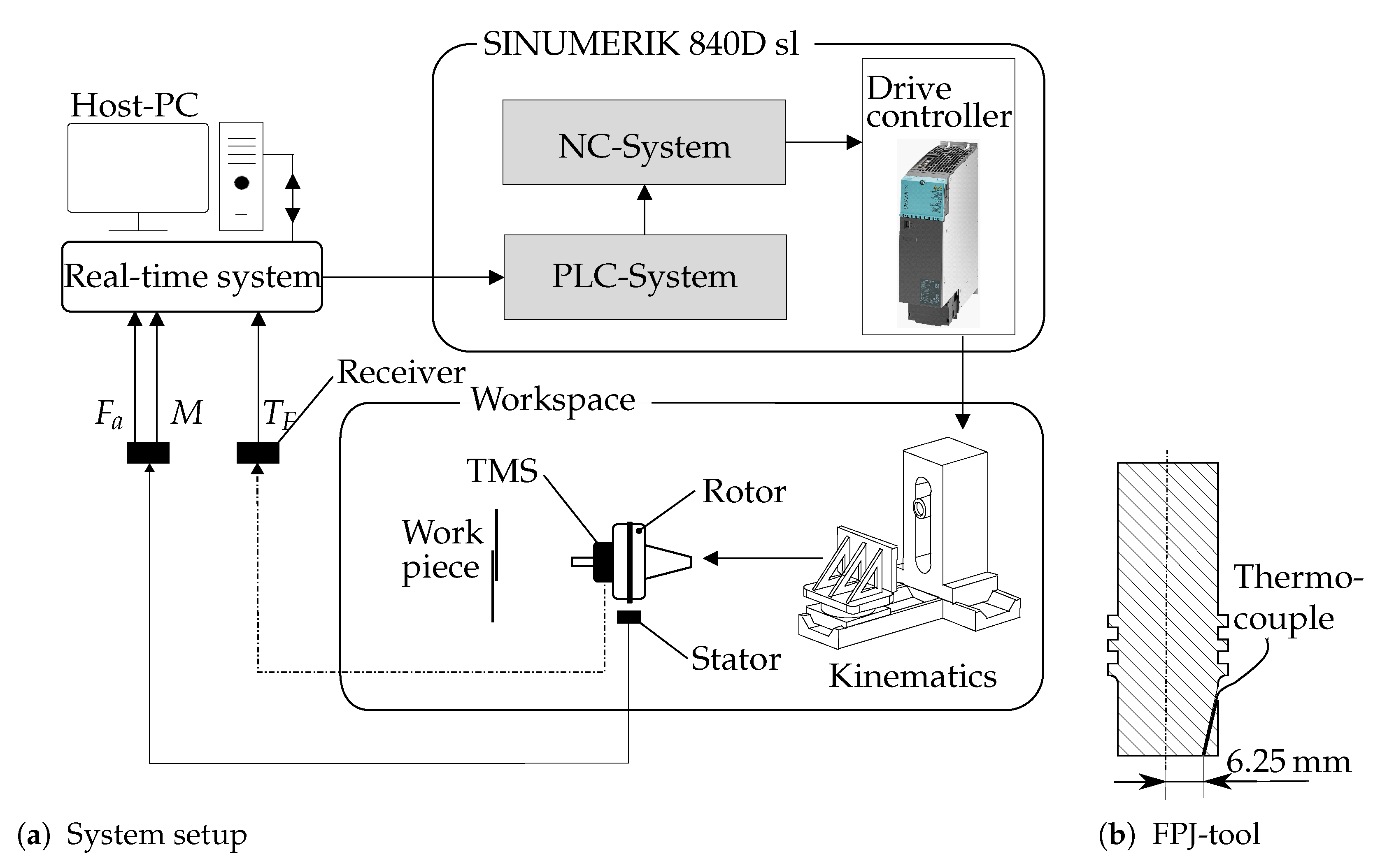
3.2. Experimental Setup

All experiments were performed on a Heller MCH 250 CNC machining center (Gebrüder Heller GmbH, Nürtingen, Germany). The machining center was equipped with the force control specified in [3]. To detect the force $F_a$, a dynamometer was placed between the tool and spindle (see Figure 3a). The temperature was measured via a thermocouple placed inside the tool (diameter of 25 $\mathrm{m}$$\mathrm{m}$) (see Figure 3b). The temperature data were transmitted via a temperature measurement system (TMS) and WLAN at 220 $\mathrm{Hz}$. More detailed information on the TMS can be found in [40]. The processing of the data and the control logic were implemented in Simulink (MATLAB 2019b, MathWorks, Natick, MA, USA) and applied to the real-time computer dSpace MicroLabBox (dSpace, Paderborn, Germany) as a C code. The signal processing of the real-time computer was performed at 10 $\mathrm{k}$$\mathrm{Hz}$.

The plunge depth was chosen as the manipulated variable for the force control. The temperature was regulated by adjusting the rotational speed.

4. System Identification

4.1. System Model

To characterize the system behavior, the approach of Taysom et al. [26] was used. This differential equation specifies the temperature generation based on the energy input by the rotation of the tool ($Q_{fric}$), the outgoing heat fluxes by conduction from the stir zone to the backing plate and the surrounding material ($Q_{cond}$), and the energy balance for the feed rate movement of the tool ($Q_{adv}$) (see Figure 4):

$$\tau \frac{d{T}_F}{dt}=Q_{fric}+Q_{cond}+Q_{adv},$$

(1)

with $\tau$ as a time constant. A more detailed description regarding the deduction is given in [26].

$Q_{fric}$ is calculated based on the generated power of the tool and is obtained by the detected torque (M) (see Figure 3) and the rotational speed of the tool (n):

$$Q_{fric}=P=M·n.$$

(2)

$Q_{cond}$ indicates the heat conduction between the friction zone and the underlying support (steel) plus the surrounding material. The area directly behind the tool is excluded. It is assumed that this area has the same temperature as the friction zone. Additionally, due to the tool’s proximity to the metallic joining partner’s edge, the heat-affected zone cannot be completely formed. This circumstance is included in the equation with the last term. Since the heat conduction through the tool is low in the quasi-static state, it can be summarized with the other terms:

$$Q_{cond}=h_1{A}_1(T_{in}-T_F)+h_2{A}_2(T_{\infty }-T_F)+h_3{A}_3(T_{\infty }-T_{in}).$$

(3)

In this equation, $A_1$ represents the area over which heat is conducted with the heat transfer coefficient $h_1$ between the friction zone and the underlying plastic component. For the conduction between the friction zone and the backing plate, the parameters $A_2$ and $h_2$ are used. The parameters $A_3$ and $h_3$ describe the not completely formed heat-affected zone.

The feed rate (v) passes material with a lower temperature into the friction zone. We assume that the material exiting the friction zone has the same temperature as the friction zone. With the material mass flow depending on the area of the friction zone ($A_F$), the density ($\rho$) of the material, and the feed rate (v), the term is as follows [26]:

$$Q_{adv}=v{A}_F\rho c_p(T_{in}-T_F).$$

(4)

The material in the vicinity of the friction zone is heated by heat conduction to the temperature $T_{in}$. This temperature influences the heat conduction away from the friction zone and the energy dissipated by the mass flow. A rising in temperature $T_F$ causes an increase in heat flux in a semi-static condition and thus a rise of $T_{in}$. The feed rate also influences the incoming temperature $T_{in}$. With higher feed rates, the energy introduced into the region becomes lower, and $T_{in}$ decreases. This linear relationship, proven in [5], can be described by the following equation:

$$T_{in}=T_F-q·v,$$

(5)

with q as a gradient coefficient [26].

By integrating Equations (2)–(4) into Equation (1), replacing $T_{in}$ with Equation (5), and weighting them with the factors a, b, and c, we obtain:

$$\tau \frac{d{T}_F}{dt}=aP+b[h_1{A}_1(T_{in}-T_F)+h_2{A}_2(T_{\infty }-T_F)+h_3{A}_3(T_{\infty }-T_{in})]+cv{A}_F\rho c_p(T_{in}-T_F)$$

(6)

Since neither the areas nor the weighting factors are straightforward to determine, we summarize them along with the material parameters resulting in the factors $c_1$, $c_2$, $c_3$, and $c_4$:

$$\begin{array}{c}\hfill \dot{T_F}=\frac{d{T}_F}{dt}=\frac{c_{1}P+c_{2}v+c_3{v}^2+c_4{T}_{\infty }-T_F}{\tau },\end{array}$$

(7)

with

$$\begin{array}{c}\hfill c_1=\frac{a}{b(h_2{A}_2+h_3{A}_3)},c_2=\frac{q(h_1{A}_1+h_3{A}_3)}{(h_2{A}_2+h_3{A}_3)},c_3=\frac{c{A}_F\rho c_{p}q}{b(h_2{A}_2+h_3{A}_3)},\end{array}$$

(8)

$$\begin{array}{r}{c}_4=1,\mathrm{and}\tau =m{c}_p.\end{array}$$

(9)

Although $c_4$ takes the value 1 according to the model, this parameter is used in the following parameterization to counteract model inaccuracies.

Following [5,26], some simplifying assumptions were made to deduce this model. First of all, it was assumed that the heat distribution within the individual zones is isothermal, i.e., the temperature gradient is zero. In addition to this, we assumed that the backing plate, due to its large thermal mass, has a constant temperature of 22 ${}^{°}\mathrm{C}$ (room temperature). This assumption is valid because of the plastic component acting as an insulating material in the FPJ process. In addition, the temperature was measured during the experiments, showing no increase in temperature. Furthermore, the aluminum-plastic composite is considered as a single unit in this assumption. Another hypothesis is that the temperature measured at the front of the tool face represents the entire joining area. Since the thermocouple location represents an average temperature (no extreme point), this assumption is certainly valid (see Figure 3b).

4.2. Parametrization of the System Model

To compensate for the model inaccuracies and the described simplifications, the model parameters were determined experimentally. Therefore, a system identification was performed based on the system Equation (7).

For this purpose, step responses of the excited system were logged. A step change of the input power, caused by a change of the rotational speed (following [3]), served as the excitation. This change was performed during the joining process while keeping the other process parameters constant (tilt angle, nominal axial force). Two changes were performed per test. During the first change, the rotational speed was increased; the second change reduced the rotational speed (and thus the applied power). With an increased rotational speed, the input power increases abruptly but declines after a couple of seconds due to the increased temperature. This increased temperature causes a softening of the workpiece material, reducing friction between the tool and the workpiece. This effect reduces the torque, the power decreases, and the temperature drops, creating a self-regulating effect as described in [3]. Nevertheless, the system behavior can be evaluated by this excitation.

Considering the feed rate’s quadratic impact in Equation (7), the tests were performed with different feed rates. The parameters were selected following the parameter range described in [5]. The axial force was regulated with the MPC developed in [3] and set to $F_{set}=1750\mathrm{N}$. The parameter sets (PS) of the experiments are listed in

Table 1. Parameter sets (PS) for the system identification with a tilt angle $\alpha$ of 2 ${}^{°}$.

Parameter Set	Feed Rate	Rotational Speed ${\mathit{n}}_{\mathbf{start}}$ at Start	Rotational Speed ${\mathit{n}}_{{\mathbf{step}}_1}$ after Step 1	Rotational Speed ${\mathit{n}}_{{\mathbf{step}}_2}$ after Step 2
	in $\frac{\mathbf{mm}}{\mathbf{min}}$	in $\frac{1}{\mathbf{min}}$	in $\frac{1}{\mathbf{min}}$	in $\frac{1}{\mathbf{min}}$
PS1	250	400	1200	700
PS2	300	400	1000	500
PS3	350	400	1200	300
PS4	400	400	800	300
PS5	450	400	1100	500
PS6	500	400	1300	400
PS7	550	400	1100	600
PS8	600	400	1000	700
PS9	650	400	1200	400
PS10	700	600	1400	700

.

To avoid disturbances during the touch-down phase and the withdrawal of the tool, we excluded the first 60 $\mathrm{m}$$\mathrm{m}$ and the last 10 $\mathrm{m}$$\mathrm{m}$ of the 200 $\mathrm{m}$$\mathrm{m}$ long seam trajectory in the evaluation, following [3]. Figure 5 shows the plot of the different relevant measured quantities for parameter set $PS5$.

To model the process, the derived differential Equation (7) was used. In this equation, the power P represents the input parameter, and the temperature $T_F$ serves as the output parameter. Combining the independent summands of the input and output variables into one term E, we get:

$$\begin{array}{c}\hfill \dot{T_F}=aP+b{T}_F+cE.\end{array}$$

(10)

During the Laplace transformation of the transfer function into a linear time-invariant (LTI) system, it becomes apparent that the error term E cannot be transferred. In order to be able to consider the disturbances, a holistic parameterization is presented in the following. For the solution, the explicit Euler method is used together with the differential Equation (7) describing the system. The explicit Euler method is characterized by a low computational time, making it possible to use it even at the high resolution of the measurement signals. This results in the following equation:

$$\begin{array}{cc}\hfill T_F(k+1)& =T_F\left(k\right)+{\dot{T}}_F\left(k\right)·\Delta t\left(k\right)\hfill \end{array}$$

(11)

$$\begin{array}{cc}& =T_F\left(k\right)+\frac{c_{1}P\left(k\right)+c_{2}v+c_3{v}^2+c_4{T}_{\infty }-T_F\left(k\right)}{\tau }·\Delta t\left(k\right)\hfill \end{array}$$

(12)

Throughout the experiments, an average room temperature of $T_{\infty }=22{}^{°}\mathrm{C}$ was assumed. Furthermore, the feed rate v was kept constant during one experiment. The method was initialized, starting with the initial temperature measurement value. Subsequently, the procedure was performed iteratively on an ongoing basis, depending on the parameter values determined by the higher-level function, until the predicted temperature curve covered the same period as the measured data of the experiment—this means a parametrization of the model with the experimental data. This procedure was performed for all tests with the same parameters. To evaluate the prediction obtained by the model, a cost function is implemented. The model’s quality was evaluated by the normalized root-mean-square error ($NRMSE$), also used as an error function:

$$\begin{array}{c}\hfill NRMS{E}_i=\frac{\left||T_{F,i}-T_{model,i}|\right|}{\left||T_{F,i}-T_{mean,i}|\right|}.\end{array}$$

(13)

By using this error, the difference between the measured temperature $T_F$ and the predicted temperature $T_{model}$ is compared to the difference between the measured and the average temperature $T_{mean}$.

To optimize the free system parameters in Equation (7), the error amount is summed up to a superordinate error and minimized over 10 trials. Constraints were also considered in terms of algebraic signs for the parameters $c_1$ (positive), $c_4$ (positive), and $\tau$ (positive). The optimized system model parameters are given in

Table 2. Parameters for the optimized system model.

Parameter	${\mathit{c}}_1$	${\mathit{c}}_2$	${\mathit{c}}_3$	${\mathit{c}}_4$	$\mathit{\tau }$
	in $\frac{{}^{°}\mathrm{C}}{\mathrm{W}}$	in $\frac{{}^{°}\mathrm{C}\mathit{·}\mathbf{min}}{\mathbf{mm}}$	in $\frac{{}^{°}\mathrm{C}\mathit{·}{\mathbf{min}}^2}{{\mathbf{mm}}^2}$	in -	in s
Value	0.250	−0.534	3.502 $·$ ${10}^{-4}$	10.813	10.096

. Figure 5c presents the measured temperature profile and the temperature profile calculated with the model.

To quantify the correlation of each test with the determined model, the ${\kappa }_{fit}$ is calculated:

$$\begin{array}{c}\hfill {\kappa }_{fit,i}=100\left(1-\frac{\left||T_{F,i}-T_{model,i}|\right|}{\left||T_{F,i}-T_{mean,i}|\right|}\right)\end{array}$$

(14)

The correlations for the experiments with the 10 initial parameter sets with the calculated trajectories based on the system model are given in

Table 3. Consistency of the model prediction with the actual measurement data.

Parameter Set	PS1	PS2	PS3	PS4	PS5	PS6	PS7	PS8	PS9	PS10
${\kappa }_{fit}$ in %	85.54	87.92	85.84	91.78	93.23	95.23	96.06	88.50	91.74	88.65

.

Considering that the machining center used does not have a power-controlled operating mode, the power term of the system equation is extended:

$$\begin{array}{c}\hfill P\left(t\right)=M\left(t\right)·n\left(t\right)·\frac{2\pi }{60s}.\end{array}$$

(15)

By reshaping and separating the differential equation into an input term (depending only on n), an output term (depending only on $T_F$), and an independent term, we get:

$$\begin{array}{cc}\hfill \frac{d{T}_F}{dt}& =\frac{c_{1}Mn\frac{2\pi }{60s}}{\tau }+\frac{T_F}{\tau }+\frac{c_{2}v+c_3{v}^2+c_4{T}_{\infty }}{\tau }.\hfill \end{array}$$

(16)

This partition can be converted into a linear state-space model format with $z\left(t\right)$ as a disturbance:

$$\begin{array}{cc}\hfill \frac{d{T}_F}{dt}& =A·T_F+B\left(M\right)·n+z\left(t\right),\hfill \end{array}$$

(17)

with A as the system matrix and $B\left(M\right)$ as the input matrix depending on the current torque.

In order to allow for a limitation of the rotational speed change by the MPC, a new state is introduced, and the manipulated variable u is redefined as the change of the rotational speed $\dot{n}$ (rotational acceleration). This modification results in a second-order system for the state-space model, with the states’ speed and temperature. The second-order state-space description has the advantage that the system automatically shows integrating behavior:

$$\begin{array}{c}\hfill \left(\begin{array}{c}\dot{n}\\ \dot{T_F}\end{array}\right)=\left(\begin{array}{cc}0& 0\\ 0.0026·M& -0.0991\end{array}\right)\left(\begin{array}{c}n\\ T_F\end{array}\right)+\left(\begin{array}{c}1\\ 0\end{array}\right)u+\left(\begin{array}{c}0\\ 1\end{array}\right)z\left(t\right).\end{array}$$

(18)

Based on this model, the temperature can be calculated, and the cross-effects of the temperature (and thus the rotational speed) on the axial force can be taken into account through the torque-dependent model. This takes into account that, at higher temperatures, the material becomes softer, the frictional force and thus the moment decreases, and the axial force decreases. In combination with the force control given in [3], a model-predictive multi-variable temperature-force control is obtained, which will be specified in more detail in the following. This combination will be called extended MPC or multi-variable control hereafter.

5. Simulation-Based Modeling of an MPC

By using the $MATLABModelPredictiveControlToolbox$, we designed an adaptive MPC in Simulink. This adaptive MPC allows consideration of the actual measured torque in the system matrix. Therefore, this approach can be used for various operating points regarding the axial force and temperature.

A dead time of $0.128$ $\mathrm{s}$ was added to the adaptive system matrix to allow for the interaction of the existing force control (see [3]) with the temperature control. The system matrix uses the current detected torque in each optimization interval and thus forms the basis of the MPC.

To configure the settings of the MPC, we first selected a sample rate at which the control block calculates the manipulated variables in advance. To obtain a high time resolution for the prediction of the immediate future, a time step size of $\Delta t=0.1\mathrm{s}$ was chosen. Due to the simulation with the system model, which showed a settling time of approximately 8 $\mathrm{s}$ when changing from 22 to 250 ${}^{°}\mathrm{C}$ rapidly, we set the prediction horizon to $n_p=80$. This high ratio of control frequency to the prediction horizon is possible due to the high computational power of the $dSpaceMicroLabBox$. If a smaller prediction horizon is used in the simulation, the resulting temperature profile hardly changes, as the difference at a lower clock rate of the control shows a more considerable influence. The control horizon $n_c$ was set to 25% of the prediction horizon to 20.

To protect the spindle from damage, the spindle power was limited. This also restricted the possible speed acceleration. To take this into account in the control algorithm, the manipulated variable was limited:

$$\begin{array}{c}\hfill u=\dot{n}=\pm 500{\min }^{-1}{\mathrm{s}}^{-1}.\end{array}$$

(19)

To be able to observe the rotational speed and restrict it in the control algorithm, the rotational speed is defined as an additional variable for reference and output. For ensuring that the rotational speed can still be set arbitrarily by the controller, its weighting in the MPC is zero. In this case, it is limited to a minimum of $n_{min}=150{\min }^{-1}$ and a maximum of $n_{max}=1200{\min }^{-1}$. With higher maximum rotational speeds, temperature overshoots increased in the experiments, and the settling period became considerably longer. Here, the simulated temperature profile of the parameterized system (Equation (18)) with the terminated MPC is shown for a constant torque of 25 $\mathrm{N}$$\mathrm{m}$ and a target temperature of 250 ${}^{°}\mathrm{C}$ (see Figure 6).

Based on this temperature control, combined with the corresponding force control from [3], and the torque-dependent system matrix, considering interactions between the individual controls, the FPJ experiments’ results can be presented in the following.

6. Experimental Analysis and Discussion

6.1. Stationary Behavior

To evaluate the performance of the extended MPC, experiments were conducted to control the temperature and the force at constant set points for the material combination PE-HD and EN AW-6082-T6. The criteria used to determine the control quality are the average values and standard deviations of the temperatures and axial forces over the joining period in the stationary case. Therefore, the first 60 $\mathrm{m}$$\mathrm{m}$ and the last 10 $\mathrm{m}$$\mathrm{m}$ of the seam length are excluded from the evaluation so as not to take into account the uncontrolled touch-down phase and the withdrawal of the tool [3].

The force control was activated after the tool has been placed on the workpiece. The combined force-temperature control is activated as soon as the feed starts. The controller was converted into C code as described in Section 3.2 and implemented on a real-time computer.

To validate the extended MPC, parameter sets with feed rates of 150 $\mathrm{m}$$\mathrm{m}$ ${\min }^{-1}$, 225 $\mathrm{m}$$\mathrm{m}$ ${\min }^{-1}$, 450 $\mathrm{m}$$\mathrm{m}$ ${\min }^{-1}$, 600 $\mathrm{m}$$\mathrm{m}$ ${\min }^{-1}$, 675 $\mathrm{m}$$\mathrm{m}$ ${\min }^{-1}$, and 750 $\mathrm{m}$$\mathrm{m}$ ${\min }^{-1}$ were used in combination with nominal temperatures of 220 ${}^{°}\mathrm{C}$, 240 ${}^{°}\mathrm{C}$, and 260 ${}^{°}\mathrm{C}$. The initial rotational speed was set to $n=500\mathrm{m}\mathrm{m}{\min }^{-1}$ in almost all experiments. Unfortunately, this starting rotational speed caused uncontrolled plunging of the tool at feed rates of 150 $\mathrm{m}$$\mathrm{m}$ ${\min }^{-1}$ due to excessive heat generation, which could not be compensated for by the controller. For this reason, a starting rotational speed of $n=200\mathrm{m}\mathrm{m}{\min }^{-1}$ was specified for this batch of experiments.

Figure 7 illustrates the temperature and force response over time for the joining process controlled by the extended adaptive MPC for a feed rate of 450 $\mathrm{m}$$\mathrm{m}$ ${\min }^{-1}$. The nominal temperature value is set here to $T_{Fset}=240{}^{°}\mathrm{C}$. All experiments showed a significant initial overshoot. The axial force was kept constant during the joining process. Only a high-frequency oscillation around the nominal value of 2000 $\mathrm{N}$ could be observed. The frequency of this oscillation corresponds to the tool’s rotational speed and can thus be related to the unbalance of the tool (see [3]).

The individual average values ($\overline{T_F}$ and $\overline{F_a}$) and the corresponding standard deviations (${\sigma }_{T_F}$ and ${\sigma }_{F_a}$) for all experiments are given in

Table 4. Mean temperature $\overline{T_F}$ in ${}^{\circ }\mathrm{C}$ and mean axial force $\overline{F_a}$ in $\mathrm{N}$, and the corresponding standard deviations (${\sigma }_{T_F}$ and ${\sigma }_{F_a}$) of the validation experiments.

v	${\mathit{T}}_{\mathit{s}\mathit{e}\mathit{t}}$	$\overline{{\mathit{T}}_{\mathit{F}}}$	${\mathit{\sigma }}_{{\mathit{T}}_{\mathit{F}}}$	$\overline{{\mathit{F}}_{\mathit{a}}}$	${\mathit{\sigma }}_{{\mathit{F}}_{\mathit{a}}}$
in mm min${}^{-1}$	in ${}^{°}\mathbf{C}$	in ${}^{°}\mathbf{C}$	in ${}^{°}\mathbf{C}$	in $\mathbf{N}$	in $\mathbf{N}$
150	220	221.7	0.86	2011.4	256.9
	240	241.6	0.79	2008.9	295.4
	260	261.8	2.19	2010.7	312.6
225	220	222.4	1.02	2013.4	201.4
	240	242.5	0.82	2020.7	257.6
	260	262.5	1.22	2019.4	325.2
450	220	221.2	2.08	1998.6	186.9
	240	241.3	3.22	2012.6	224.9
	260	258.4	4.50	2003.3	220.6
600	220	219.2	3.23	1973.1	260.8
	240	236.9	5.30	2001.1	261.3
	260	255.0	6.84	1983.8	279.8
675	220	217.4	3.57	1997.1	196.8
	240	249.6	5.31	1999.0	227.7
	260	254.5	5.05	1987.6	231.4
750	220	216.3	3.88	2002.5	219.1
	240	234.1	5.40	1983.2	229.0
	260	251.3	8.44	2004.2	249.4

. It can be seen that the temperature and the force can be controlled very well. However, with higher feed rates, the average temperature deviation increases. This can be explained by the low dynamics of the process. In these cases, the settling of the temperature took longer, so it is included in the specified measuring frame. Therefore, the results of the feed rates 675 $\mathrm{m}$$\mathrm{m}$ ${\min }^{-1}$ and 750 $\mathrm{m}$$\mathrm{m}$ ${\min }^{-1}$ show significantly poorer results. However, at all feed rates below 600 $\mathrm{m}$$\mathrm{m}$ ${\min }^{-1}$, even for those not included in the parametrization, there is good consistency between the nominal temperature and nominal force within a low standard deviation.

6.2. Performance under Model Uncertainties

Thus far, we have used the same material combination to validate the controller as for its design. The following section discusses the results of a change of materials (plastic part and aluminum sheet). This modification can be interpreted as a model uncertainty due to the changed thermal conductivity, stiffness, and material geometries. Furthermore, the nominal temperature was adjusted to the respective plastic.

Following [3,10], feed rates of 225 $\mathrm{m}$$\mathrm{m}$ ${\min }^{-1}$, 240 $\mathrm{m}$$\mathrm{m}$ ${\min }^{-1}$, 400 $\mathrm{m}$$\mathrm{m}$ ${\min }^{-1}$, 560 $\mathrm{m}$$\mathrm{m}$ ${\min }^{-1}$, and 600 $\mathrm{m}$$\mathrm{m}$ ${\min }^{-1}$ were tested for the combination of PA6-GF30 with EN AW-6082-T6. The nominal temperatures were set to 260 ${}^{°}\mathrm{C}$ and 290 ${}^{°}\mathrm{C}$. The applied axial force was 2000 $\mathrm{N}$. Like for the other experiments, the steady-state was also quantified starting from 60 $\mathrm{m}$$\mathrm{m}$ after the start. The obtained results are presented in

Table 5. Average temperature $\overline{T_F}$ in ${}^{\circ }\mathrm{C}$ and average axial force $\overline{F_a}$ of the transfer tests with the material combination PA6-GF30 with EN AW-6082 T6.

v	${\mathit{T}}_{\mathit{s}\mathit{e}\mathit{t}}$	$\overline{{\mathit{T}}_{\mathit{F}}}$	${\mathit{\sigma }}_{{\mathit{T}}_{\mathit{F}}}$	$\overline{{\mathit{F}}_{\mathit{a}}}$	${\mathit{\sigma }}_{{\mathit{F}}_{\mathit{a}}}$
in mm min${}^{-1}$	in ${}^{°}\mathbf{C}$	in ${}^{°}\mathbf{C}$	in ${}^{°}\mathbf{C}$	in $\mathbf{N}$	in $\mathbf{N}$
225	260	263.0	1.52	1991.3	423.5
	290	292.6	2.40	2025.5	211.7
240	260	263.6	2.34	2010.6	391.9
	290	291.8	1.84	2014.8	218.5
400	260	261.2	4.21	2009.9	254.3
	290	289.6	7.00	1997.4	220.1
560	260	255.5	4.72	2001.5	234.4
	290	286.9	8.49	2046.9	274.1
600	260	253.5	4.94	1974.6	248.2
	290	284.1	7.86	1999.6	297.1

.

The results demonstrate that the control is still capable of operating effectively regardless of this introduced model uncertainty and the increased temperatures. Although the plastic’s thermal properties differ significantly from those of PE-HD, the altered thermal conductivity is not significant enough to affect the process to such an extent that the controller is no longer usable. Nevertheless, there is a slight decrease in the control quality. The axial force can be controlled very well with this material combination.

To introduce more significant uncertainties, experiments were conducted with a combination of PPS-CF and EN AW-2024-T3. The nominal temperatures were set to 300 ${}^{°}\mathrm{C}$ and 340 ${}^{°}\mathrm{C}$, the feed rates to 300 $\mathrm{m}$$\mathrm{m}$ ${\min }^{-1}$ and 450 $\mathrm{m}$$\mathrm{m}$ ${\min }^{-1}$, and the contact pressure to 2500 $\mathrm{N}$. Besides the changed thermal properties of the two joining partners, the dimensions (thicknesses) with $2.17$ $\mathrm{m}$$\mathrm{m}$ (plastic part) and 2 $\mathrm{m}$$\mathrm{m}$ (aluminum sheet) are significantly smaller than those of the material combination considered initially. The results of the mean values and standard deviations are shown in

Table 6. Average temperature $\overline{T_F}$ in ${}^{°}\mathrm{C}$ and average axial force $\overline{F_a}$ of the transfer tests with the material combination PPS-CF with EN AW-2024-T3.

v	${\mathit{T}}_{\mathit{s}\mathit{e}\mathit{t}}$	$\overline{{\mathit{T}}_{\mathit{F}}}$	${\mathit{\sigma }}_{{\mathit{T}}_{\mathit{F}}}$	$\overline{{\mathit{F}}_{\mathit{a}}}$	${\mathit{\sigma }}_{{\mathit{F}}_{\mathit{a}}}$
in mm min${}^{-1}$	in ${}^{°}\mathbf{C}$	in ${}^{°}\mathbf{C}$	in ${}^{°}\mathbf{C}$	in $\mathbf{N}$	in $\mathbf{N}$
300	300	306.8	11.0	2510.8	296.9
	340	346.1	15.2	2515.9	246.7
450	300	302.7	11.3	2515.7	221.1
	340	336.5	16.3	2511.7	128.6

.

According to the results, similar deviations of the nominal temperature prevail for the material combination PPS-CF and EN AW-2024-T3 as for the other material combinations. However, the standard deviation is considerably higher. One reason for this is that a small oscillation around the nominal value occurs, especially at these high temperatures. This oscillation does not subside and can be related to the deviations of the system model used in the MPC. These differences are caused by the aluminum sheet used having a significantly lower thickness and thus a smaller thermal mass, meaning that it heats up faster for the same power input. In addition, the PPS-CF used has a significantly lower thermal conductivity, which additionally changes the system.

Overall, it can be concluded that the extended adaptive model predictive force-temperature control is valid for a large operating range but is limited by excessive model uncertainties. This large operating range can be explained by the torque-dependent linearization and the robustness of the control approach. Based on this control, the temperature between the tool and the aluminum surface can be controlled. However, since the temperature $T_J$, which cannot be measured in situ, is crucial for the bond strength, a model will be presented in the following, with which the temperature in the plastic can be calculated and thus indirectly regulated.

7. FDM Multi-Layer Temperature Distribution Model

7.1. FDM Multi-Layer Model

Structure of the Model

After demonstrating that the temperature ($T_F$) between the tool and the workpiece surface can be controlled, this section deals with the temperature distribution in the plastic-metal bond during the process.

Meyer et al. [5] showed that the measurable temperature ($T_F$) between the tool and the workpiece surface can be regulated by the variables n and v. These variables also influence the temperature in the plastic material ($T_J$). This temperature can only be measured at certain points when a thermocouple is placed in the interface between the metal and plastic. The temperature difference $\Delta T$ between $T_F$ and $T_J$ also corresponds to the manipulated variables n and v. The authors showed that the temperature $T_J$ in the plastic is decisive for the bond strength. Since this temperature cannot be measured in situ, a method for an in-process calculation of the temperature distribution in the plastic-metal composite is presented in the following.

The plastic-metal bond, including a backing plate, can be abstracted as a layered system in a simplified way. This layer system, hereafter referred to as a multi-layer system, consists of three parts: The aluminum sheet, the plastic joining partner, and the backing plate. It is assumed that heat transfer in the multi-layer system occurs exclusively by thermal conduction. The convection appearing on the free surface of the backing plate is neglected. The convection between the molten plastic and the aluminum plate is also not simulated. The thermal radiation in and around the body is not considered in the model due to its minor nature.

Each layer is considered as a flat plate with a finite thickness and temperature-dependent material properties. The heat flow in the FPJ process is modeled with a transient heat conduction equation due to the relatively short duration in the process. For the multi-layer system in general, while assuming that there are no mass transport and heat radiation losses per layer, this results in:

$$\begin{array}{c}\hfill T=T(x,y,z,t)\end{array}$$

(20)

and

$$\begin{array}{c}\hfill c_p\rho \frac{\partial T}{\partial t}-\lambda {\nabla }^{2}T=0,\end{array}$$

(21)

with T as temperature, $x,y$, and z as coordinates, t as time, ∇ as nabla operator, $\lambda$ as thermal conductivity, $\rho$ as density, and $c_p$ as specific heat capacity.

To calculate the temperature distribution in real-time, the 3D case is abstracted as a 1D model along the z-axis. This abstraction enables a more efficient and faster calculation of the temperature in the cross-section of the layered system. Thus, the transient heat conduction equation per layer in the 1D case results in:

$$\frac{\partial T}{\partial t}=\alpha \left(T\right)·\frac{{\partial }^{2}T}{\partial t^2},$$

(22)

with

$$\alpha \left(T\right)=\frac{\lambda \left(T\right)}{\rho \left(T\right)·c_p\left(T\right)},$$

(23)

with T as temperature, $\alpha$ as heat transfer coefficient, and t as time.

To solve the heat conduction equation numerically, the forward Euler Method is used. Here, the differential Equation (22) is replaced by a finite difference method (FDM):

$$\begin{array}{cc}\hfill T_i(t+\Delta t)& =T_i\left(t\right)+\frac{d{T}_i}{dt}\Delta t\hfill \end{array}$$

(24)

$$\begin{array}{cc}\hfill \frac{d{T}_i}{dt}& =\alpha \left(T_i\right)·\left(\frac{T_{i+1}-T_i}{d{z}^2}-\frac{T_i-T_{i-1}}{d{z}^2}\right)\hfill \end{array}$$

(25)

with $T_i$ equal to the temperature at location i, $\Delta z$ equal to the integration span in the z-direction, and $\Delta t$ equal to the integration span in time.

Using this equation, each layer in the multi-layer system can be modeled. The output layers of the superordinate layer serve as input for the next layer. Thermal transfer resistances can be considered during the transfer from the output layer to the input layer. In the following, an ideal heat transfer between the individual layers is assumed.

The aluminum layer is based on the temperature-dependent material model developed by [41]. The temperature-dependent modeling is required here since the aluminum heats up from the initial temperature of approx. 20 ${}^{°}\mathrm{C}$ up to approx. 450 ${}^{°}\mathrm{C}$.

The data of the plastic joining partner (PE-HD) is based on selected models in the literature. The density is calculated with the material model from [42]. The thermal conductivity and the specific heat capacity were calculated depending on the results of [43].

In contrast to the two joining partners, the backing plate (steel) is heated only slightly during the process. For this reason, a temperature-dependent material model was not used here, and fixed values were specified [44]:

$$\begin{array}{cc}\hfill {\rho }_{Steel}& =7850\mathrm{k}\mathrm{g}{\mathrm{m}}^{-3},\hfill \end{array}$$

(26)

$$\begin{array}{cc}\hfill c_{P_{Steel}}& =486\mathrm{J}{\mathrm{kg}}^{-1}{\mathrm{K}}^{-1},\mathrm{and}\hfill \end{array}$$

(27)

$$\begin{array}{cc}\hfill {\lambda }_{Steel}& =49.8\mathrm{W}{\mathrm{m}}^{-1}{\mathrm{K}}^{-1}.\hfill \end{array}$$

(28)

In addition to the simplifications mentioned above, an ambient temperature and an initial temperature of each of the joining partners of 22 ${}^{°}\mathrm{C}$ were assumed. The simulation time is adjusted to the tool’s traverse time and thus to the feed rate. It is assumed that the temperature is applied only by the tool, and the measured temperature $T_F$ is the same for the whole area between the tool and the aluminum surface. The effective duration of the temperature is thus calculated as:

$$t_{sim}=d_{tool}/v_{tool},$$

(29)

with $t_{sim}$ as the simulation time, $d_{tool}$ as the diameter of the tool, and $v_{tool}$ as the feed rate of the tool.

Each layer is abstracted with 50 individual differences, allowing a resolution of 100 $\mathsf{\mu }$$\mathrm{m}$. The time scale resolution is $0.001$ $\mathrm{s}$. With this model and the assumptions made, the temperature in the bond can be calculated.

7.2. Validation of the FDM Multi-Layer Model

Since the temperature in the plastic component cannot be measured directly, cross-sections of the bonded specimens were made to measure the melt layer thickness (see [5]). By using this melt layer, it is possible to detect the depth to which the melting temperature occurred. Simultaneously, the melt layer thickness was calculated using the 1D FDM model and compared with the measured results (see Figure 8).

The results show that the 1D FDM model can be used to calculate the melt layer thickness, and thus the temperature in the plastic component. In the intermediate region of approx. 0.3$\mathrm{m}$$\mathrm{m}$ to 1$\mathrm{m}$$\mathrm{m}$, the prediction correlates well with the measured data. However, there are mostly deviations above 1 $\mathrm{m}$$\mathrm{m}$. These differences can be explained by specific presumptions, like the hypothesis of an ideal heat transfer. Furthermore, this deviation may occur due to the 1D modeling, since heat fluxes in the x- and y-direction are not considered here.

Overall, it can be concluded that the model represents the temperature distribution within the bond well. A detailed 3D model might offer even more accurate results, but the 1D model can be used as a feed-forward control for the extended MPC to indirectly regulate the temperature $T_J$.

8. Summary and Conclusions

The purpose of this study was to present a model-based system identification for designing a model predictive temperature control, extending the existing force control to a multi-variable closed-loop system. By using a torque-based system architecture, it was possible to model the interactions between the two manipulated variables over a broad parameter domain. Furthermore, it was shown that the extended multi-variable control can be applied to various material combinations with a low standard deviation of $\le 10\mathrm{K}$ and $\le 330\mathrm{N}$ for the material combination of PE-HD and EN AW-6082-T6. In the end, we presented a 1D FDM model to calculate the temperature distribution in the bond. Due to the simplifications made, this FDM model can serve as a feed-forward control for the designed control loop, allowing indirect control of the joining zone’s temperature. Altogether, the effective implementation of a holistic process control was achieved, and the following main conclusions (C1–C4) can be formulated:

C1 

Due to the modified differential equation, the fundamental thermal process evolution of the FPJ process can be described.

C2 

By using the torque-based system matrix, the interactions between the temperature and the axial force can be modeled. Thus, it is possible to linearize the state-space model around the respective operating point, covering a large operating range.

C3 

The adaptive MIMO-MPC based on this torque-based system matrix is suitable for controlling the temperature and axial force for FPJ.

C4 

The 1D FDM temperature model is appropriate as a feed-forward control for the MIMO-MPC to calculate the temperature in the bond during the process with an accuracy of r = 0.93.

This work provides the fundamentals for controlling the temperature and the axial force in the bond. Based on these results, the pressure and temperature-dependent properties of plastics can be considered in future studies. In addition, the control concept developed can also be used for FSW. However, this hypothesis remains to be verified.

References

1. El Rayes, M.M.; Soliman, M.S.; Abbas, A.T.; Pimenov, D.Y.; Erdakov, I.N.; Abdel-mawla, M.M. Effect of Feed Rate in FSW on the Mechanical and Microstructural Properties of AA5754 Joints. Adv. Mater. Sci. Eng. 2019, 2019, 1–12. [Google Scholar] [CrossRef] [Green Version]
2. Meyer, S.P.; Wunderling, C.; Zaeh, M.F. Friction press joining of dissimilar materials: A novel concept to improve the joint strength. In Proceedings of the 22nd international ESAFORM Conference on Material Forming: ESAFORM 2019, Vitoria-Gasteiz, Spain, 8–10 May 2019; p. 050031. [Google Scholar] [CrossRef]
3. Meyer, S.P.; Bernauer, C.J.; Grabmann, S.; Zaeh, M.F. Design, evaluation, and implementation of a model-predictive control approach for a force control in friction stir welding processes. Prod. Eng. 2020, 54, 20. [Google Scholar] [CrossRef]
4. Taysom, B.S.; Sorensen, C.D.; Hedengren, J.D. A comparison of model predictive control and PID temperature control in friction stir welding. J. Manuf. Process 2017, 29, 232–241. [Google Scholar] [CrossRef]
5. Meyer, S.P.; Wunderling, C.; Zaeh, M.F. Influence of the laser-based surface modification on the bond strength for friction press joining of aluminum and polyethylene. Prod. Eng. 2019, 13, 721–730. [Google Scholar] [CrossRef] [Green Version]
6. Nagatsuka, K.; Yoshida, S.; Tsuchiya, A.; Nakata, K. Direct joining of carbon-fiber–reinforced plastic to an aluminum alloy using friction lap joining. Compos. Part B Eng. 2015, 73, 82–88. [Google Scholar] [CrossRef]
7. Goushegir, S.M.; dos Santos, J.F.; Amancio-Filho, S.T. Friction Spot Joining of aluminum AA2024/carbon-fiber reinforced poly(phenylene sulfide) composite single lap joints: Microstructure and mechanical performance. Mater. Des. 2014, 54, 196–206. [Google Scholar] [CrossRef]
8. Buffa, G.; Baffari, D.; Campanella, D.; Fratini, L. An Innovative Friction Stir Welding Based Technique to Produce Dissimilar Light Alloys to Thermoplastic Matrix Composite Joints. Procedia Manuf. 2016, 5, 319–331. [Google Scholar] [CrossRef] [Green Version]
9. Okada, T.; Uchida, S.; Nakata, K. Effect of anodizing on direct joining properties of aluminium alloy and plastic sheets by friction lap joining. Weld. Int. 2018, 32, 85–94. [Google Scholar] [CrossRef]
10. Wirth, F.X.; Fuchs, A.N.; Rinck, P.; Zaeh, M.F. Friction Press Joining of Laser-Texturized Aluminum with Fiber Reinforced Thermoplastics. Adv. Mater. Res. 2014, 966–967, 536–545. [Google Scholar] [CrossRef]
11. Han, S.C.; Wu, L.H.; Jiang, C.Y.; Li, N.; Jia, C.L.; Xue, P.; Zhang, H.; Zhao, H.B.; Ni, D.R.; Xiao, B.L.; et al. Achieving a strong polypropylene/aluminum alloy friction spot joint via a surface laser processing pretreatment. J. Mater. Sci. Technol. 2020, 50, 103–114. [Google Scholar] [CrossRef]
12. Fuchs, A.N.; Wirth, F.X.; Rinck, P.; Zaeh, M.F. Laser-generated Macroscopic and Microscopic Surface Structures for the Joining of Aluminum and Thermoplastics using Friction Press Joining. Phys. Procedia 2014, 56, 801–810. [Google Scholar] [CrossRef] [Green Version]
13. Liu, F.C.; Liao, J.; Nakata, K. Joining of metal to plastic using friction lap welding. Mater. Des. 2014, 54, 236–244. [Google Scholar] [CrossRef]
14. Gebhard, P.; Zaeh, M.F. Force Control Design for CNC Milling Machines for Friction Stir Welding. In Proceedings of the 7th International Symposium on Friction Stir Welding; TWI Ltd.: Cambridge, UK, 2008. [Google Scholar]
15. Longhurst, W.R.; Strauss, A.M.; Cook, G.E.; Cox, C.D.; Hendricks, C.E.; Gibson, B.T.; Dawant, Y.S. Investigation of force-controlled friction stir welding for manufacturing and automation. Proc. Inst. Mech. Eng. Part B J. Eng. Manuf. 2010, 224, 937–949. [Google Scholar] [CrossRef]
16. Ziegler, J.G.; Nichols, N.B. Optimum Settings for Automatic Controllers. Trans. ASME 1942, 64, 759–768. [Google Scholar] [CrossRef]
17. Zhao, X.; Kalya, P.; Landers, R.G.; Krishnamurthy, K. Design and Implementation of a Nonlinear Axial Force Controller for Friction Stir Welding Processes. In Proceedings of the 2007 American Control Conference, New York, NY, USA, 9–13 July 2007; pp. 5553–5558. [Google Scholar] [CrossRef]
18. Zhao, X.; Kalya, P.; Landers, R.G.; Krishnamurthy, K. Empirical Dynamic Modeling of Friction Stir Welding Processes. J. Mater. Process. Technol. 2009, 131, 021001. [Google Scholar] [CrossRef]
19. Davis, T.A.; Shin, Y.C.; Yao, B. Observer-based adaptive robust control of friction stir welding axial force. In Proceedings of the 2010 IEEE/ASME International Conference on Advanced Intelligent Mechatronics, Montreal, QC, Canada, 6–9 July 2010; pp. 1162–1167. [Google Scholar] [CrossRef]
20. Zhao, S.; Bi, Q.; Wang, Y. An axial force controller with delay compensation for the friction stir welding process. Int. J. Adv. Manuf. Technol. 2016, 85, 2623–2638. [Google Scholar] [CrossRef]
21. Fehrenbacher, A.; Smith, C.B.; Duffie, N.A.; Ferrier, N.J.; Pfefferkorn, F.E.; Zinn, M.R. Combined Temperature and Force Control for Robotic Friction Stir Welding. J. Manuf. Sci. Eng. 2014, 136, 1. [Google Scholar] [CrossRef]
22. Fehrenbacher, A.; Pfefferkorn, F.E.; Zinn, M.R.; Ferrier, N.J.; Duffie, N.A. Closed-loop control of temperature in friction stir welding. In Proceedings of the 7th International Symposium on Friction Stir Welding; TWI Ltd.: Cambridge, UK, 2008. [Google Scholar]
23. Fehrenbacher, A.; Duffie, N.A.; Ferrier, N.J.; Pfefferkorn, F.E.; Zinn, M.R. Toward Automation of Friction Stir Welding Through Temperature Measurement and Closed-Loop Control. J. Manuf. Sci. Eng. 2011, 133. [Google Scholar] [CrossRef]
24. Fehrenbacher, A.; Cole, E.G.; Zinn, M.R.; Ferrier, N.J.; Duffie, N.A.; Pfefferkorn, F.E. Towards Process Control of Friction Stir Welding for Different Aluminum Alloys. In Friction Stir Welding and Processing VI; Mishra, R.S., Ed.; Wiley: Hoboken, The Netherlands, 2011; Volume 51, pp. 381–388. [Google Scholar] [CrossRef]
25. Bachmann, A.; Zaeh, M.F. Pyrometer-Assisted Temperature Control in Friction Stir Welding. In Proceedings of the 11th International Friction Stir Welding Symposium; TWI Ltd.: Cambridge, UK, 2016. [Google Scholar]
26. Taysom, B.S.; Sorensen, C.D.; Hedengren, J.D. Dynamic modeling of friction stir welding for model predictive control. J. Manuf. Process 2016, 23, 165–174. [Google Scholar] [CrossRef]
27. Völz, A. Modellprädiktive Regelung Nichtlinearer Systeme mit Unsicherheiten [Engl. Model Predictive Control of Nonlinear Systems with Uncertainties], 1st ed.; Springer: Wiesbaden, Germany, 2016. [Google Scholar] [CrossRef]
28. S-POLYTEC GmbH. Technical Data Sheet: PE-HD. Available online: https://www.s-polytec.com/media/attachment/file/d/a/data_sheet_pe-hd_sheets.pdf (accessed on 9 July 2019).
29. Schäfer, C.; Bryant, J.S.; Osswald, T.A.; Meyer, S.P. Micropelletization of Virgin and Reycled Thermoplasitc Materials. In Annual Technical Conference (ANTEC) of the Society of Plastics Engineers (SPE); Society of Plastics Engineers: Anaheim, CA, USA, 2017; Volume 2017. [Google Scholar]
30. Schäfer, C.; Meyer, S.P.; Osswald, T.A. A novel extrusion process for the production of polymer micropellets. Polym. Eng. Sci. 2018, 44, 1391. [Google Scholar] [CrossRef]
31. Karagöz, İ. An effect of mold surface temperature on final product properties in the injection molding of high-density polyethylene materials. Polym. Bull. 2020. [Google Scholar] [CrossRef]
32. Meyer, S.P.; Jaeger, B.; Wunderling, C.; Zaeh, M.F. Friction stir welding of glass fiber-reinforced polyamide 6: Analysis of the tensile strength and fiber length distribution of friction stir welded PA6-GF30. IOP Conf. Ser. Mater. Sci. Eng. 2019, 480, 012013. [Google Scholar] [CrossRef]
33. Gemmel Metalle & Co. GmbH. Technical Data Sheet: AlMgSi1 F30. Available online: https://www.gemmel-metalle.de/downloads/Legierungsbeschreibung_AlMgSi1_F30.pdf (accessed on 9 July 2019).
34. Heckert, A.; Zaeh, M.F. Laser surface pre-treatment of aluminum for hybrid joints with glass fiber reinforced thermoplastics. J. Laser Appl. 2015, 27, 29005. [Google Scholar] [CrossRef]
35. Ensinger Ltd. TECAMID 6 GF30 Black—Stock Shapes. Available online: https://www.ensingerplastics.com/de-de/halbzeuge/produkte/pa6-tecamid-6-gf30-black (accessed on 9 July 2019).
36. TenCate Advanced Composites BV. Data Sheet: Cetex TC1100 PPS. Available online: https://www.toraytac.com/media/221a4fcf-6a4d-49f3-837f-9d85c3c34f74/smphpw/TAC/Documents/Data_sheets/Thermoplastic/UD%20tapes,%20prepregs%20and%20laminates/Toray-Cetex-TC1100_PPS_PDS.pdf (accessed on 9 July 2019).
37. André, N.M.; Goushegir, S.M.; dos Santos, J.F.; Canto, L.B.; Amancio-Filho, S.T. Friction Spot Joining of aluminum alloy 2024-T3 and carbon-fiber-reinforced poly(phenylene sulfide) laminate with additional PPS film interlayer: Microstructure, mechanical strength and failure mechanisms. Compos. Part B Eng. 2016, 94, 197–208. [Google Scholar] [CrossRef]
38. Lugauer, F.P.; Kandler, A.; Meyer, S.P.; Wunderling, C.; Zaeh, M.F. Induction-based joining of titanium with thermoplastics. Prod. Eng. 2019, 13, 409–424. [Google Scholar] [CrossRef] [Green Version]
39. Batz+Burgel GmbH & Co. KG. Data Sheet: EN AW-2024. Available online: https://batz-burgel.com/en/metal-trading/aluminium-product-range/en-aw-2024/ (accessed on 9 July 2019).
40. Costanzi, G.; Bachmann, A.; Zäh, M.F. Entwicklung eines FSW-Spezialwerkzeugs zur Messung der Schweißtemperatur. In Proceedings of the DVS Congress 2017, Düsseldorf, Germany, 26–29 September 2017. [Google Scholar]
41. Liebl, S.; Stadter, C.; Ganser, A.; Zaeh, M.F. Numerical simulation of laser beam welding using an adapted intensity distribution. J. Laser Appl. 2017, 29, 022405. [Google Scholar] [CrossRef]
42. Olabisi, O.; Simha, R. Pressure-Volume-Temperature Studies of Amorphous and Crystallizable Polymers. I. Experimental. Macromolecules 1975, 8, 206–210. [Google Scholar] [CrossRef]
43. Rauwendaal, C. Polymer Extrusion, 5th ed.; Hanser eLibrary, Hanser: München, Germany, 2014; pp. 234–249. [Google Scholar]
44. MatWeb. Available online: http://www.matweb.com/search/datasheet.aspx?matguid=cbe4fd0a73cf4690853935f52d910784 (accessed on 29 January 2021).
45. DIN EN 573-3:2018-12. Aluminium and Aluminium Alloys—Chemical Composition and form of Wrought Products—Part 3: Chemical Composition and form of Products; Beuth Verlag GmbH: Berlin, Germany, 2018. [Google Scholar] [CrossRef]
46. Otto Fuchs, K.G. Technical Information: Material Data Sheet Aluminium. Available online: https://www.otto-fuchs.com/en/service/material-information.html (accessed on 9 July 2019).
Figure 1. The friction press joining process with its forces and temperatures during the process (based on [5]).
Metals 11 00502 g001
Figure 2. Closed-loop control system with an MPC controller, including an optimizer and a process model.
Metals 11 00502 g002
Figure 3. Illustration of the system setup for the implementation of the force and the temperature control (a), and a cross section of the used tool with inserted thermocouple at 6.25 m m from the center (b).
Metals 11 00502 g003
Figure 4. Different thermal areas of the simplified thermal system.
Metals 11 00502 g004
Figure 5. Plot of the measured parameters n, P, and T F for experiment P S 5 , and the predicted temperature T m o d e l from the system model.
Metals 11 00502 g005
Figure 6. Temperature control simulation with the parameterized system and a constant torque of 25 N m .
Metals 11 00502 g006
Figure 7. Temperature and force responses of the complete joining process regulated by the extended MPC with F a s e t = 2000   N , v = 450   m m   min 1 , and T F s e t = 240   ° C .
Metals 11 00502 g007
Figure 8. Comparison of the measured and the predicted melt layer thicknesses (r = 0.93)
Metals 11 00502 g008