Non- and Quasi-Equilibrium Multi-Phase Field Methods Coupled with CALPHAD Database for Rapid-Solidification Microstructural Evolution in Laser Powder Bed Additive Manufacturing Condition

Abstract

A solidification microstructure is formed under high cooling rates and temperature gradients in powder-based additive manufacturing. In this study, a non-equilibrium multi-phase field method (MPFM), based on a finite interface dissipation model, coupled with the Calculation of Phase Diagram (CALPHAD) database, was developed for a multicomponent Ni alloy. A quasi-equilibrium MPFM was also developed for comparison. Two-dimensional equiaxed microstructural evolution for the Ni (Bal.)-Al-Co-Cr-Mo-Ta-Ti-W-C alloy was performed at various cooling rates. The temperature-γ fraction profiles obtained under 10⁵ K/s using non- and quasi-equilibrium MPFMs were in good agreement with each other. Over 10⁶ K/s, the differences between the non- and quasi-equilibrium methods grew as the cooling rate increased. The non-equilibrium solidification was strengthened over a cooling rate of 10⁶ K/s. Columnar-solidification microstructural evolution was performed at cooling rates of 5 × 10⁵ K/s to 1 × 10⁷ K/s at various temperature gradient values under a constant interface velocity (0.1 m/s). The results show that, as the cooling rate increased, the cell space decreased in both methods, and the non-equilibrium MPFM was verified by comparing with the quasi-equilibrium MPFM. Our results show that the non-equilibrium MPFM showed the ability to simulate the solidification microstructure in powder bed fusion additive manufacturing.

1. Introduction

Additive manufacturing is used to produce complex three-dimensional machine parts by feeding alloy powder layer by layer. The powder layer surface is irradiated by a high-power laser, melted and solidified in every feeding. This process is called laser powder bed fusion (LPBF). The mechanical properties of machine parts fabricated by LPBF often supersede those produced by conventional casting methods due to the unique solidification microstructure [1]. The short diameter (100 µm) and high moving speeds (0.1–1 m/s orders) of the laser spot enable high cooling rates and temperature gradients around the melting pool. These conditions lead to a microstructure that results in exceptional mechanical properties [2,3,4]. Many researchers have reported that the solidification microstructure obtained by LPBF was produced using cooling ranges from 10⁴ K/s to 10⁶ K/s and temperature gradients from 10⁵ K/s to 10⁷ K/s [5,6,7]. Rapid solidification is desired to design the LPBF process parameters to obtain a precise microstructure. However, analyzing high-speed rapid solidification in LPBF is experimentally challenging. Therefore, numerical methodologies can help to unravel the mechanism of rapid solidification in LPBF.

Many Finite Element Method (FEM) analyses have been performed to show the temporal temperature distributions around a moving laser spot [8,9,10]. Furthermore, Computational Fluid Dynamics (CFD) analyses have been performed to obtain not only the temperature distribution but also the fluid flow in the melt pool by considering the free surface affected by Marangoni convection. Macroscopic solidifications have been attempted by weak coupling with the temporal temperature distribution or by the Volume of Fluid (VOF) method in CFD analysis [11,12]. However, these numerical techniques do not provide information about microstructural evolution and cellular or dendric growths because constitutional cooling is not rigorously estimated due to its large-scale discretization for the description of solute diffusion boundary layers. Moreover, cellular automaton applied to relatively short-length scales provide cellular or dendritic growth, considering the constitutional undercooling [13,14]. Recently, columnar-to-equiaxed transition analysis was successfully applied to rapid solidification conditions in LPBF. The multi-phase field method (MPFM) was used along with weak coupling analyses, macroscopic thermal and/or fluid dynamics and microstructural evolution [15,16,17,18]. Local equilibrium and quasi-equilibrium assumptions are usually made regarding cellular automaton or the MPFM [19], respectively. These assumptions could be applied to rapid solidification in LPBF [20].

It is well known that nickel alloy, as a kind of austenitic alloy, is highly susceptible to hot cracking, such as solidification cracking during welding. The brittle temperature range (BTR) is an important factor to evolute the susceptibility to cracking. BTR is defined by the temperature difference between the liquidus and solidus temperatures and is usually evaluated by Scheil model calculation [21]. The Scheil model is based on the local equilibrium assumption with regard to the interface between solid and liquid phases. It is considered that there is difference of BTR values between the local equilibrium of the Scheil model and the non-equilibrium of rapid solidification of LPBF. A high accuracy estimation of BTR is demanded to determine the cracking susceptibility of Ni alloy in LPBF. The purpose of this study is to develop a numerical simulation method to obtain practical solute partitioning in the solid–liquid interface and determine its morphology under rapid solidification in multi-component system. We focused on the cracking susceptibility of precipitation-strengthened Ni alloy in LPBF. In the present study, a common nickel-based superalloy, Inconel (INC) 738LC, was chosen as the model alloy, which has excellent creep and corrosion resistance and strength at high temperatures [22,23,24]. However, when an LPBF process is used to fabricate a part with INC738LC, cracking often occurs. In order to suppress such cracking behaviors, microstructure control and optimization are important approaches, and phase field simulation can be a powerful tool for that purpose.

The finite interface dissipation model for the phase-field method (PFM) was proposed by Steinbach et al. [25,26]. This model permits the PFM to describe the non-equilibrium solute distribution with a new parameter called permeability at the interface region. By using this model, the MPFM has been extended to a multi-component system consisting of substitutional and interstitial elements in combination with the Calculation of Phase Diagram (CALPHAD) database. Recently, Karayagiz et al. performed solidification microstructure analysis using non-equilibrium finite interface dissipation and MPFM for a Ni-Nb binary system by weakly coupling with FEM thermal analysis in LPBF [27]. They found that the segregation coefficient value simulated by the non-equilibrium MPFM was close to the quasi-equilibrium MPFM as the permeability value increased. This coincidence was confirmed for the segregation coefficient from one-dimensional simulation.

To date, the literature on solidification microstructure evolution using the MPFM has usually studied binary or ternary systems. In this study, we developed non- and quasi-equilibrium MPFMs coupled with the CALPHAD database for Ni alloys for multi-component system. Next, non- and quasi-equilibrium MPFMs were compared to equiaxed microstructure evolution simulations at various cooling rates. The coincidence between non- and quasi-equilibrium MPFMs was studied in terms of solid fraction-temperature relations from the two-dimensional equiaxed simulation in practical multi-component system. Finally, columnar microstructure evolutions performed by both MPFMs in the same steady interface under various cooling rates and temperature gradients were compared and discussed. It is noted that although the microstructures of metals and alloys consist of grains, cell growth in grains is discussed as microstructure evolution in the present study.

2. Model Description and Computational Procedure

2.1. Non- and Quasi-Equilibrium Multi-Phase Field Method

The finite interface dissipation model proposed by Steinbach and Zhang [23] was adapted to develop the non-equilibrium MPFM. This MPFM equation has the same structure as the conventional MPFM. The conventional MPFM equation is based on a quasi-equilibrium assumption that is defined by the parallel tangent law between Gibbs free energy curves varying with solute compositions of two or more phases according to the KKS model [28]. This restriction is not necessary for the non-equilibrium MPFM. The MPFM equation is described by using the double-obstacle potential for consistency, as follows:

$$\frac{\partial {\varphi }_{\alpha }}{\partial t}={\displaystyle \sum }_{\beta =1}^N\frac{K_{\alpha \beta }}{N}\left\{{\displaystyle \sum }_{k=1}^N\left[\left(\frac{{\pi }^2}{{\delta }^2}{\varphi }_k+{\nabla }^2{\varphi }_k\right)\left({\sigma }_{\beta k}-{\sigma }_{\alpha k}\right)\right]+\frac{2\pi }{\delta }\sqrt{{\varphi }_{\alpha }{\varphi }_{\beta }}\mathsf{\Delta }{G}_{\alpha \beta }\right\}$$

(1)

where ${\varnothing }_{\alpha }$, ${\sigma }_{\beta k}$, $K_{\alpha \beta }$, δ and $N$ are the phase order ($0\leqq {\varnothing }_{\alpha }\leqq 1$), interface energy, interface mobility, interface width and number of phases or grains constructing the interface, respectively. $\mathsf{\Delta }{G}_{\alpha \beta }$ is the interface driving force between phases α and β. Non-equilibrium MPFM is expressed as

$$\mathsf{\Delta }{G}_{\alpha \beta }=f_{\beta }-f_{\alpha }-{\displaystyle \sum }_{i=1}^{n-1}{\displaystyle \sum }_{\zeta =1}^N{\varphi }_{\zeta }{\tilde{\mu }}_{\zeta }^i\left(c_{\beta }^i-c_{\alpha }^i\right)$$

(2)

where $f_{\alpha }$, $f_{\beta }$, $c_{\alpha }^i$, $c_{\beta }^i$, ${\tilde{\mu }}_{\zeta }^i$ and $n$ are the Gibbs free energy density of phases α and β, the molar fraction of element $i$ in phases α and β, the diffuse potential—that is, the gradient of the Gibbs free energy tangent line for element $i$—the composition direction in phase ζ and number of (solute and solvent Ni) elements in the system, respectively. In the conventional MPFM, the diffuse potential values of all phases at a point at the interface become equal, ${\tilde{\mu }}_{\gamma }^i={\tilde{\mu }}_{}^i$. The driving force, $\mathsf{\Delta }{G}_{\alpha \beta }$, is expressed as

$$\mathsf{\Delta }{G}_{\alpha \beta }=f_{\beta }-f_{\alpha }-{\displaystyle \sum }_{i=1}^{n-1}{\tilde{\mu }}_{}^i\left(c_{\beta }^i-c_{\alpha }^i\right)$$

(3)

The conventional MPFM driving force can be considered as a special case of the non-equilibrium MPFM.

The interface mobility correction is essential to precisely control interface motion. Interface mobility values were corrected according to Equation (16) in [29] and Equation (35) in [30] for quasi and non-equilibrium MPFMs, respectively. The anti-trapping current was also found using Equation (29) in [30]. These equations were derived for the double-obstacle potential of the phase-field equation.

The evolution equations of solute compositions in the interface region were proposed by Zhang et al. [29], as follows:

$${\dot{c}}^i=\nabla ·{\displaystyle \sum }_{\alpha =1}^N\left[{\varphi }_{\alpha }{\displaystyle \sum }_{j=1}^{n-1}{D}_{ij}^{\alpha }\nabla c_{\alpha }^j\right]+{\displaystyle \sum }_{\beta =1}^N{P}_{\alpha \beta }^i{\varphi }_{\beta }\left({\tilde{\mu }}_{\beta }^i-{\tilde{\mu }}_{\alpha }^i\right)-{\displaystyle \sum }_{\beta =1}^N{\dot{\varphi }}_{\beta }\left(c_{\beta }^i-c_{\alpha }^i\right)$$

(4)

where $D_{ij}^{\alpha }$ is the diffusivity matrix in phase α. $P_{\alpha \beta }^i$ is a new parameter named the interface permeability that acts as a strength-partitioning solute element $i$ between phases α and β. Equation (4) is separated into two steps according to our previous study [31]:

$${\dot{c}}^i=\nabla ·{\displaystyle \sum }_{\alpha =1}^N\left[{\varphi }_{\alpha }{\displaystyle \sum }_{j=1}^{n-1}{D}_{ij}^{\alpha }\nabla c_{\alpha }^j\right]$$

(5)

$${\dot{c}}^i={\displaystyle \sum }_{\beta =1}^N{P}_{\alpha \beta }^i{\varphi }_{\beta }\left({\tilde{\mu }}_{\beta }^i-{\tilde{\mu }}_{\alpha }^i\right)-{\displaystyle \sum }_{\beta =1}^N{\dot{\varphi }}_{\beta }\left(c_{\beta }^i-c_{\alpha }^i\right)$$

(6)

Equation (5) is the diffusion equation in the interface region as in the conventional MPFM. Equation (6) is called the interface partitioning rate equation in this study. Equation (6) is implicitly solved to be convergent at each time step by the successive relaxation method. Moreover, in the quasi-equilibrium MPFM, partitioned solute element compositions were obtained by the parallel tangent law:

$${\tilde{\mu }}_{\alpha }^j\left(c_{\alpha }^i\right)={\tilde{\mu }}_{\beta }^j\left(c_{\beta }^i\right)$$

(7)

Equation (7) was solved by the Newton–Rapson method. The different parts of the numerical program code for non- and quasi-equilibrium MPFMs were solved by Equations (6) and (7), respectively. Other parts were common in both MPFM codes. Therefore, microstructural evolution differences between non- and quasi-equilibrium MPFMs were obtained.

Anisotropic properties of dendritic or cellular growth were considered in Equation (1). A two-dimensional model [32] was employed to define the interfacial energy and the interface mobility between liquid and solid phases using

$${\sigma }_{\alpha \beta }\left(\theta \right)={\overline{\sigma }}_{\alpha \beta }\left[1+{\epsilon }_4\cos \left(4\theta \right)\right]$$

(8)

$$K_{\alpha \beta }={\overline{K}}_{\alpha \beta }\left[1+{\epsilon }_4\cos \left(4\theta \right)\right]$$

(9)

respectively, where $\alpha =\mathrm{FCC}$ and $\beta =\mathrm{Liquid}$. θ is the angle of the normal vector on the interface and is given by $\theta ={\tan }^{-1}\left\{\left(\partial {\varnothing }_{\alpha }/\partial y\right)/\left(\partial {\varnothing }_{\alpha }/\partial x\right)\right\}$. ${\epsilon }_4$ is the coefficient of four-fold symmetry, where 0.0167 and 0.25 were selected for the interfacial energy and the interface mobility, respectively. The anisotropy functions were not given for the interface between $\gamma$ grains in the present calculations.

2.2. Sublattice Model of γ in the CALPHAD Framework

INC738LC alloy, the principal components of which are Ni(Bal.)-Al-Co-Cr-Mo-Ta-Ti-W-C, was selected to simulate the solidification microstructure of γ (FCC phase). The thermodynamics values, Gibbs free energy and chemical potential of FCC and liquid phases were numerically provided from the CALPHAD database. In this study, the Ni database of Thermo-Calc [33], TCNI9 [34], was applied to obtain the thermodynamics values using Thermo-Calc TQ-Interface [35], which is a FORTRAN subroutine module. The numeric modules of the TQ-Interface should be used for MPFM calculation to reduce the CPU time. As this quick numeric module does not directly provide chemical potential values, the sublattice structure has to be considered in programming to estimate thermodynamic values.

The CALPHAD crystal structure of γ, consisting of Ni(Bal.)-Al-Co-Cr-Mo-Ta-Ti-W-C, was described by substitutional and interstitial sublattices, [Al, Co, Cr, Mo, Ni, Ta, Ti, W]m[C, Va]l, where m and l are units for the FCC phase and Va indicates a vacancy at the C site in the second sublattice. Chemical potentials for elements, ${\mu }_{\mathrm{C}}$, ${\mu }_{\mathrm{j}}$, j = Al, Co, Cr, Mo, Ni, Ta, Ti and W in the FCC phase were described as

$$\left\{\begin{array}{c}{\mu }_{\mathrm{C}}=\frac{1}{l}\left(\frac{\partial G^{\prime }}{\partial y_{\mathrm{C}}}-\frac{\partial G^{\prime }}{\partial y_{\mathrm{Va}}}\right)\\ {\mu }_{\mathrm{j}}=\frac{1}{m}{G}^{\prime }-\frac{1}{l}\frac{c_{\mathrm{C}}}{1-c_{\mathrm{C}}}\left(\frac{\partial G^{\prime }}{\partial y_{\mathrm{C}}}-\frac{\partial G^{\prime }}{\partial y_{\mathrm{Va}}}\right)-\frac{1}{1-c_{\mathrm{C}}}{\displaystyle {\displaystyle \sum }_{\mathrm{i},\mathrm{j}\ne \mathrm{C}}}{x}_{\mathrm{i}}\left(\frac{\partial G^{\prime }}{\partial y_{\mathrm{i}}}-\frac{\partial G^{\prime }}{\partial y_{\mathrm{j}}}\right)\\ \mathrm{j}=\mathrm{Al}, \mathrm{Co}, \mathrm{Cr}, \mathrm{Mo}, \mathrm{Ni}, \mathrm{Ta}, \mathrm{Ti}, \mathrm{W}\end{array}\right.$$

(10)

where $y_{\mathrm{c}}$, $y_{\mathrm{i}}$ are the site fractions of the element in the sublattices, and $G^{\prime }$ is the Gibbs free energy for the total effective site number in the unit lattice. The TQ-interface provides a differential of $G^{\prime }$ with site fraction, $\partial G^{\prime }/\partial y_{\mathrm{i}}$, by reading parameter values from the CALPHAD sublattice model database. The derivation of Equation (10) is explained in Appendix A. Equation (10) can be promptly expanded to any kind or number of element systems and provides fast computation capability. This derivation procedure is promptly applied to more than two sublattice structures—e.g., $\gamma \prime$ (order–disorder FCC_L12 phase)—as explained in Appendix A.

2.3. Computational Methods and Common Conditions

Equations (1) and (5) were solved using the two-dimensional finite difference method by forwarding in time and centering in space. A constant grid width, $\mathsf{\Delta }x$, and time step, $\mathsf{\Delta }t$, were applied. $\mathsf{\Delta }t$ was estimated by using maximum stability limitation values according to the diffusivity obtained by the diffusion equation and interface mobility and interfacial energy in the MPFM equation. The interface region width, $\delta$, was five times the grid width in all calculations in this study. The interface region was defined as the FCC phase order (${\varnothing }_{\mathrm{FCC}}$) value from $2.5\times {10}^{-5}$ to $\left(1-2.5\times {10}^{-5}\right)$. Bulk liquid and FCC phases were defined by $0\leqq {\varnothing }_{\mathrm{FCC}}< 2.5\times {10}^{-5}$ and $\left(1-2.5\times {10}^{-5}\right)< {\varnothing }_{\mathrm{FCC}}\leqq 1$, respectively.

The initial Ni alloy composition was selected as Ni(Bal.)-3.2Al-0.1C-8.5Co-16.3Cr-1.65Mo-1.8Ta-3.22Ti-2.7W (wt.%) of INC738LC in this study. The as-cast microstructure contained almost only γ (FCC phase) grains based on our experimental measurements. The initial solidified γ (FCC phase) appeared at 1630.9 K using the equilibrium property calculation using Thermo-Calc software. Initial temperature values were set at 1621 K (undercooled state). The diffusivity of γ varied with temperature (Arrhenius equation) and was estimated using the diffusion database of Thermo-Calc. The diffusivity of liquid, $D_{\mathrm{L}}$, was set as 2.0 × 10⁻⁹ m²/s for all calculations in this study.

2.4. Permeability Value

Zhang et al. proposed the interface permeability equation related to the bulk diffusion mobilities as follows [29]:

$$P_{\mathrm{FCC}, \mathrm{Liquid}}^i=8\frac{{\varphi }_{\mathrm{FCC}}{V}_m^{\mathrm{FCC}}{\tilde{M}}_i^{\mathrm{FCC}}+{\varphi }_{\mathrm{Liquid}}{V}_m^{\mathrm{Liquid}}{\tilde{M}}_i^{\mathrm{Liquid}}}{\alpha \delta }$$

(11)

where ${\tilde{M}}_i^{\mathrm{FCC}}$ and ${\tilde{M}}_i^{\mathrm{Liquid}}$ are the diffusion mobilities of element i in bulk FCC and liquid phases, respectively, and $V_m^{\mathrm{FCC}}$ and $V_m^{\mathrm{Liquid}}$ are the molar volumes of FCC and liquid phases, respectively. $a$ is the physical interface length at the atomic scale. Equation (11) shows an interpolating formulation by two terms, which vary with the phase order ${\varnothing }_{\mathrm{FCC}}$ where ${\varnothing }_{\mathrm{Liquid}}=1-{\varnothing }_{\mathrm{FCC}}$. The former (FCC) and the latter (liquid) were evaluated as follows: diffusion mobility values were estimated using the diffusion mobility database MOBNI5 for the equilibrium compositions of the alloy Ni(Bal.)-3.2Al-0.1C-8.5Co-16.3Cr-1.65Mo-1.8Ta-3.22Ti-2.7W (wt.%) at 1626K. ${\tilde{M}}_i^{\mathrm{FCC}}$ values were obtained as $1.72\times {10}^{-18}~4.02\times {10}^{-17} {\mathrm{m}}^2·\mathrm{mol}/\mathrm{J}/\mathrm{s}$ for the substitutional elements and $2.03\times {10}^{-14} {\mathrm{m}}^2·\mathrm{mol}/\mathrm{J}/\mathrm{s}$ for the interstitial element C. ${\tilde{M}}_i^{\mathrm{Liquid}}$ values were obtained as $1.14~2.10\times {10}^{-13} {\mathrm{m}}^2·\mathrm{mol}/\mathrm{J}/\mathrm{s}$ for the substitutional elements and $6.91\times {10}^{-13} {\mathrm{m}}^2·\mathrm{mol}/\mathrm{J}/\mathrm{s}$ for the interstitial element C. The molar volumes $V_m^{\mathrm{FCC}}$ and $V_m^{\mathrm{Liquid}}$ were approximated as $8.0\times {10}^{-6} {\mathrm{m}}^3/\mathrm{mol}$. The physical interface length was assumed to be 2 nm. The former (FCC) term, $8·V_m^{\mathrm{FCC}}{\tilde{M}}_i^{\mathrm{FCC}}/a/\delta$, led to $1.01\times {10}^{-6}~2.36\times {10}^{-5} {\mathrm{m}}^3/\mathrm{J}/\mathrm{s}$ for the substitutional elements and $1.19\times {10}^{-2} {\mathrm{m}}^3/\mathrm{J}/\mathrm{s}$ for the interstitial element C. The latter term (liquid), $8·V_m^{\mathrm{Liquid}}{\tilde{M}}_i^{\mathrm{Liquid}}/a/\delta$, led to $7.30\times {10}^{-2}~0.13 {\mathrm{m}}^3/\mathrm{J}/\mathrm{s}$ for the heavy elements and $0.44 {\mathrm{m}}^3/\mathrm{J}/\mathrm{s}$ for the light element C. Furthermore, the maximum number of the permeability $P_{\mathrm{FCC}, \mathrm{Liquid}}^i$ to maintain numerical stability was found as ~$4\times {10}^{-5} {\mathrm{m}}^3/\mathrm{J}/\mathrm{s}$ by applying the same permeability value to all elements. This number had the same order as the former (FCC) term, $8·V_m^{\mathrm{FCC}}{\tilde{M}}_i^{\mathrm{FCC}}/a/\delta$, for the substitutional elements and was smaller than that of the interstitial element C or the permeability defined by the liquid, $8·V_m^{\mathrm{Liquid}}{\tilde{M}}_i^{\mathrm{Liquid}}/a/\delta$. If the solute element partition were controlled by reducing the diffusion mobility between the two phases, the permeability would be decided by the minimized value. The following solidification microstructure evolution was calculated based on a permeability value of ${10}^{-5} {\mathrm{m}}^3/\mathrm{J}/\mathrm{s}$ in this study.

3. Equiaxed Microstructure Evolution

3.1. Specific Model Conditions for Equiaxed Microstructure Evolution

The region was set as a square with 200 × 200 grid points. The grid width was 2.0 × 10⁻⁸ m. The initial γ grains, whose number was set as seven, were randomly distributed for nucleation. Their diameter was defined as one grid size. The grain crystalline directions were also randomly provided. The interfacial energy and the interface mobility between the liquid phase and γ were set to $0.2 {\mathrm{J}/\mathrm{m}}^2$ and $2.0\times {10}^{-8} {\mathrm{m}}^4/\mathrm{J}/\mathrm{s}$, respectively. The permeability $P_{\mathrm{FCC}, \mathrm{Liquid}}^i$ value was defined as $2\times {10}^{-5} {\mathrm{m}}^3/\mathrm{J}/\mathrm{s}$ for the non-equilibrium MPFM calculations. A uniform temperature (zero temperature gradient) was assumed. The calculations were performed at four cooling rates: 10⁴ K/s, 10⁵ K/s, 10⁶ K/s and 10⁷ K/s. The initial temperature values were set at 1621 K to avoid initial γ grains from disappearing by the Gibbs–Thomson effect. Periodic boundary conditions were adapted for solving the MPFM and diffusion equations. The same conditions were supplied for the non- and quasi-equilibrium calculations.

3.2. Results and Discussion

Figure 1 and Figure 2 show the solidification microstructure distributions at a cooling rate of 10⁵ K/s with non- and quasi-equilibrium calculations, respectively, at 0.06 ms, showing the solute concentration and γ grain distributions. The solute diffusion and partitioning around the advancing interface between liquid and solid phases were precisely calculated for all elements. The segregation between grain interfaces was also confirmed. The random anisotropy between the liquid phase and γ grains was activated. We found that the solidification in the quasi-equilibrium MPFM (Figure 2) was more advanced than that in the non-equilibrium MPFM (Figure 1).

The solidification microstructure evolutions were compared by changing the cooling rate for the two models. Figure 3 shows the temporary solidification microstructure distributions at a cooling rate of 10⁴ K/s using non- and quasi-equilibrium MPFMs. The solute element C was selected to visualize the solute concentration distribution. γ grain sizes obtained from the two MPFMs were similar. The solute distributions were also very close to each other. Figure 4 shows the temporary solidification microstructure distributions at a cooling rate of 10⁷ K/s. The solidification obtained using the quasi-equilibrium MPFM advanced more compared with that using the non-equilibrium MPFM. Thus, the difference in the solidification rate between non- and quasi-equilibrium MPFMs increased as the cooling rate increased under the same conditions.

Figure 5 shows the relations of temperature with the FCC phase (γ) area fraction for cooling rates of 10⁴ K/s, 10⁵ K/s, 10⁶ K/s and 10⁷ K/s for non- and quasi-equilibrium MPFMs and the Scheil model (Thermo-Calc) calculation considering carbon back-diffusion. The difference between the temperature-FCC phase fraction profiles obtained from Scheil and MPFM calculations increased with the increased cooling rate. Under relatively low cooling rates, solidification interface motion was mainly controlled by the constitutional under the cooling of the solute diffusion. If the cooling rate gradually decreased to zero, the solute concentration distribution around the interface neared that obtained by the Scheil model, which was assumed to be infinite under zero solute diffusivity for the liquid and solid, respectively, except for the infinite diffusivity of C in the solid. The results at 10⁴ K/s were close to those obtained by the Scheil model, except for the initial undercooling period. Thermal undercooling corresponded to the majority of the solidification interfaces at an increasing cooling rate [36]. Thus, the growth rate under a higher cooling rate accelerated in the early stage and strongly decelerated as it neared the local equilibrium at the interface in the final stage.

It can be seen that the temperature-FCC phase (γ) fraction profiles between the non-equilibrium and quasi-equilibrium MPFMs almost coincide with each other at cooling rates lower than 10⁵ K/s. Furthermore, this difference gradually grows for cooling rates higher than 10⁶ K/s at which the quasi-equilibrium MPFM growth rate is larger than the non-equilibrium MPFM growth rate. The non-equilibrium solidification is strengthened at above 10⁶ K/s in the present alloy composition. It is well known that the non-equilibrium distribution (segregation) coefficient increases with the growth rate [37]. Karayagiz et al. reported that the non-equilibrium distribution coefficient, $k_v$, increased with the growth rate due to the columnar microstructure evolution using the non-equilibrium MPFM for the Ni-Nb binary system [27]. They also found that the $k_v$ of the non-equilibrium MPFM calculation asymptotically approached that of the quasi-equilibrium MPFM with an increase in permeability. As permeability is a strength factor for segregation partitioning, it is expected that the temperature-FCC phase fraction profile obtained by the non-equilibrium MPFM will be close to that obtained by the quasi-equilibrium MPFM profile at increased permeability, as the same tendency was confirmed for the γ-α transformation [38].

Figure 6 shows the temperature-FCC phase fraction profiles of the non-equilibrium and quasi-equilibrium MPFMs, which varied with permeability values of $1\times {10}^{-5} {\mathrm{m}}^3/\mathrm{J}/\mathrm{s}$, $2\times {10}^{-5} {\mathrm{m}}^3/\mathrm{J}/\mathrm{s}$ and $4\times {10}^{-5} {\mathrm{m}}^3/\mathrm{J}/\mathrm{s}$ at a cooling rate of 10⁷ K/s. It can be seen that the non-equilibrium profiles gradually moved closer to the quasi-equilibrium profiles. At a permeability of $4\times {10}^{-5} {\mathrm{m}}^3/\mathrm{J}/\mathrm{s}$, the profiles were almost the same for the two methods. It was confirmed that the permeability $4\times {10}^{-5} {\mathrm{m}}^3/\mathrm{J}/\mathrm{s}$ was the maximum value because calculations in the condition of the permeability over this value caused numerical instability. As explained in Section 2.3, the permeability value was determined with digit-order precision. However, the evaluation of the non-equilibrium property for different cooling rates is available in the present non-equilibrium MPFM calculation procedure.

4. Columnar Microstructure Evolution

In the previous section, the permeability value, $4\times {10}^{-5} {\mathrm{m}}^3/\mathrm{J}/\mathrm{s}$, was estimated to give an approximately equal equiaxed-solidification fraction rate for non- and quasi-equilibrium MPFM calculations at a cooling rate of 10⁷ K/s. The microstructure evolution difference for the two methods is confirmed in this section at a steady growth rate, $\overline{v}=0.1 \mathrm{m}/$s, for various cooling rates and temperature gradients using the permeability value, $4\times {10}^{-5} {\mathrm{m}}^3/\mathrm{J}/\mathrm{s}$.

4.1. Specific Model Conditions for Columnar Microstructure Evolution

The grid width was 1.0 × 10⁻⁸ m, which was defined to place four grids in the diffusion boundary layer length of the liquid side, ${\delta }_{\mathrm{L}}=2D_{\mathrm{L}}/\overline{v}=4\times {10}^{-8}\mathrm{m}$. The cooling rate and the temperature gradient for the vertical direction were uniformly applied. The four combinations of the cooling rate and the temperature gradient were set as shown in

Table 1. Variations in cooling rate and temperature gradient at a steady interface growth rate (0.1 m/s).

Case	Cooling Rate, R (K/s)	Temperature Gradient, G (K/m)
(a)	5 × 105	5 × 106
(b)	1 × 106	1 × 107
(c)	5 × 106	5 × 107
(d)	1 × 107	1 × 108

. The calculation region was set as a rectangle with 250 × 1500 grid points. However, 250 × 2000 grid points were applied to Case (a) to obtain steady growth. The initial γ grain was placed at the bottom as a film. The initial bottom temperature was set at 1621 K as for the previous equiaxed microstructure evolution condition. The time step of 1.0 × 10⁻⁸ s was adopted in all cases (Table 1). The symmetrical boundary conditions for the MPFM and diffusion equations were adapted for horizontal and vertical directions. The other conditions were the same as those defined in Section 2.3 and Section 3.1.

4.2. Experimental Conditions

A cylindrical Inconel 738LC specimen with dimensions of 10 mm in diameter and 10 mm in height was fabricated by selective laser melting (SLM) in order to evaluate an actual cell structure. A commercial SLM device (SLM 280, SLM Solutions GmbH, Germany) was used. A laser power of 300 W and scan velocity of 900 mm/s were applied with the spot diameter of 80 µm. The pitch width and single-layer thickness were 100 µm and 30 µm, respectively. The specimen was cut and embedded into an epoxy mount and polished for cross-sectional microstructure observation by a scanning electron microscope (SEM, JSM-7200F, JEOL Ltd., Japan).

4.3. Results and Discussion

Figure 7 shows the snapshots of the microstructures obtained by the quasi-equilibrium MPFM calculations for conditions listed in Table 1. All cases reached steady cellular microstructures with boundaries parallel to the vertical direction, and the cell spaces were maintained. The average cell space decreased from cases (a) to (d) with the increased cooling rate and temperature gradient. Three growth stages were obtained: initial growth, accelerated growth with fine cellular segregation and decelerated growth forming the steady cell microstructure. Figure 8 shows the interface moving velocity values with time for all cases. Each curve contains two inflection points, which are the boundaries between the three growth stages. In the second stage, the fine cellular segregation growth is accompanied by hard competition, which causes the segregation lines to fluctuate and disappear. In the second stage, the interface velocity continues to accelerate alongside the steady growth rate of 0.1 m/s. After the maximum velocity is reached, in the third stage, a steady cellular microstructure is gradually constructed with the deceleration of the interface velocity. The length of the second stage is shortened from Cases (a) to (c). However, in Case (d), there is no obvious transformation from the second to third stages. The fine segregation microstructure promptly becomes a steady state, as evidenced by the smaller overshot velocity of Case (d) in Figure 8. It is considered that Case (d) is in transition from cellular to planar interface growth.

The overshot velocity value from the steady velocity of 0.1 m/s monotonically increases with the decreased cooling rate. In the second stage, the fine cellular segregation period, the length increases with increased overshot velocity. These tendencies are likely to be caused by the mandatory quasi-equilibrium assumption at the interface. The solute partitioning estimated by the quasi-equilibrium leads to a large interface driving force. The interface velocity continues to accelerate over a steady velocity to the beginning of the competitive fine cellular segregation. Moreover, the balance between the solute partitioning, cell spacing length and solute undercooling starts to be formed according to the classical solidification theory based on the local equilibrium [39]. Then, the interface velocity decreases and reaches a steady state by constructing a regular cellular microstructure. A higher cooling rate can reach a steady undercooling temperature more quickly. Thus, the second stage period of a higher-cooling-rate case is shorter than that of the lower-cooling-rate case.

Figure 9 shows the snapshots of solidification microstructure distributions at Al concentrations (molar fraction) obtained by the non-equilibrium MPFM under the conditions listed in Table 1. The interface moving velocity values over time are shown in Figure 10. The interface velocities of Cases (a) and (b) do not reach the steady value of 0.1 m/s. However, the steady cellular microstructures with constant cell spacing are formed at an early stage in all cases. The average cell space length decreases as the cooling rate and temperature gradient increase from cases (a) to (d). This is larger than that of the quasi-equilibrium MPFM case in all cases. The second stage of microstructure evolution constructed with competitive fine cellular segregation is not obvious in the non-equilibrium MPFM cases in Figure 9. The cellular microstructure promptly forms after only a few cellular growth competitions followed by the initial planer interface being broken in all cases. The overshooting tendency in Figure 10 is the opposite of that seen in Figure 8. In particular, in cases (a) and (b), overshooting does not appear. In Cases (c) and (d), cell growth competitions are weak, regardless of the overshooting of the interface velocity. These results are considered to be led by the interface non-equilibrium assumption, which causes a lower driving force of constitutional undercooling due to the weaker solute portioning in the moving interface than the quasi-equilibrium assumption.

The diffusional and thermal undercooling values were estimated as shown in Figure 11. The liquidus temperatures, $T_0$ and $T^{*}$, for the initial alloy concentration and the cell tip concentration were obtained by Thermo-Calc, respectively. The undercooling temperature due to the curvature of the cell tip was not considered in this discussion because of the similarity in tip shapes in Figure 7 and Figure 9. Figure 12 shows the diffusional and thermal undercooling values in the cell tips in Figure 7 and Figure 9. The thermal undercooling values are much larger than the diffusional undercooling values. It is well known that the fraction of thermal undercooling increases with the increased cooling rate. It is reported that the fraction of thermal undercooling becomes approximately 80% at a cooling rate of 100 K/s and a temperature gradient of 1000 K/m for the Al-Cu alloy [36]. Figure 12 qualitatively agrees with this relation. The diffusional undercooling difference between non-equilibrium and quasi-equilibrium MPFMs is not large because liquid solute compositions at the tips have almost the same values, and liquidus temperature differences are less than five degrees (Figure 7 and Figure 9). Furthermore, the thermal undercooling of the non-equilibrium MPFM is about two to three times larger than that of the quasi-equilibrium MPFM in each case. Thus, in the non-equilibrium MPFM, the solidification microstructure evolution is driven more by thermal undercooling than that in the quasi-equilibrium MPFM at a high cooling rate. The necessity of high thermal undercooling in the non-equilibrium MPFM arises from its weaker solute partitioning, which leads to weak constitutional undercooling. Then, the weak constitutional driving force is compensated by the thermal undercooling to achieve a steady interface velocity (0.1 m/s). In the previous equiaxed microstructure evolution, the permeability value is calibrated to adjust the solidification phase fraction varying with temperature between non- and quasi-equilibrium MPFMs. However, it is found that the difference in the columnar microstructure evolution between two MPFMs appears despite using the calibrated permeability.

In Figure 9, the number of cells in case (a) of the non-equilibrium MPFM is rather small. It is considered to be more affected by the horizontal boundary condition than other cases. An additional calculation using twice the number of horizontal grid points–500–was performed to reduce the impact of the boundary condition. The snapshot of solidification microstructure distributions with different Al concentrations (molar fraction) is shown in Appendix B. The number of cells increased from 1.3 per 2.5 μm in Figure 9 to 3.5 per 5 μm in Appendix B. The average cell space changed from 1.92 μm to 1.43 μm. In the following method, we use the revised cell space of 1.43 μm. The interface moving velocity and diffusional undercooling at cell tip were confirmed to be approximately same as the previous results in Figure 10 and Figure 12, respectively.

Table 2. Average cell space (μm) at a steady interface moving velocity if 0.1 m/s. Numbers in parentheses are ratios of the cell space in which the space of case (a) is defined as a unit.

Case	Non-Equilibrium MPFM	Quasi-Equilibrium MPFM
(a)	1.43 (1)	0.45 (1)
(b)	0.89 (0.62)	0.36 (0.8)
(c)	0.45 (0.32)	0.29 (0.64)
(d)	0.31 (0.22)	0.16 (0.35)

shows the approximate average cell space values of cases (a), (b), (c) and (d) for non-and quasi-equilibrium MPFMs. The ratios of the cell space in which the space of case (a) is defined as a unit are shown in parentheses. The ratios in the non-equilibrium MPFM decrease rapidly compared to those in the quasi-equilibrium MPFM. Karayagiz et al. reported a solidification microstructure simulation for the Ni-3.2 at.%Nb system by comparing with experimental measurements with various cooling rates and temperature gradients [27]. They estimated the ratio of the cell space as 0.35 for cooling rates from $5\times {10}^5 \mathrm{K}/\mathrm{s}$ to $5\times {10}^6 \mathrm{K}/\mathrm{s}$, which corresponds to cases (a) to (c) in Table 2. This is quite close to the ratio–0.32–obtained by the non-equilibrium MPFM. Furthermore, the average cell space in the quasi-equilibrium MPFM sees a smaller decreasewith the cooling rate from cases (a) to (c).

Figure 13 shows an as-cast microstructure obtained experimentally for the same alloy composition. The cooling rate is estimated to vary in the same range as in Table 1, from ${10}^5 \mathrm{K}/\mathrm{s}$ to ${10}^6 \mathrm{K}/\mathrm{s}$ orders of digits, by thermal FEM analysis [40]. It can be seen that the morphology in Figure 13 is constructed by a cellular structure with a cell space of around 1 μm. The quasi-equilibrium MPFM cell spaces in Figure 7 or Table 2 are too narrow compared to those in Figure 13. The fluctuated fine cellular segregation area, which is obtained by the quasi-equilibrium MPFM, is not identified in Figure 13. It is considered that the present non-equilibrium MPFM can more accurately simulate rapid solidification in powder bed fusion processes than in quasi-equilibrium MPFM.

5. Conclusions

In this work, the non-equilibrium multi-phase field method using the finite interface dissipation model and the quasi-equilibrium multi-phase field method, coupled with the CALPHAD database, were employed for Ni(Bal.)-Al-Co-Cr-Mo-Ta-Ti-W-C. Equiaxed and columnar solidification microstructure evolutions of γ were performed in LPBF thermal conditions with these methods. The main results and conclusion are summarized as follows:

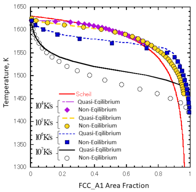
• The temperature-γ fraction relationships under a cooling rate of 10⁵ K/s for non- and quasi-equilibrium MPFMs in the two-dimensional equiaxed simulations were in good agreement with each other. They were quite close to the Scheil model profile at 10⁴ K/s.
• The differences between non- and quasi-equilibrium methods grew with the cooling rate. The non-equilibrium solidification tendency was strengthened with the cooling rate of 10⁶ K/s.
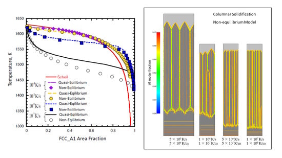
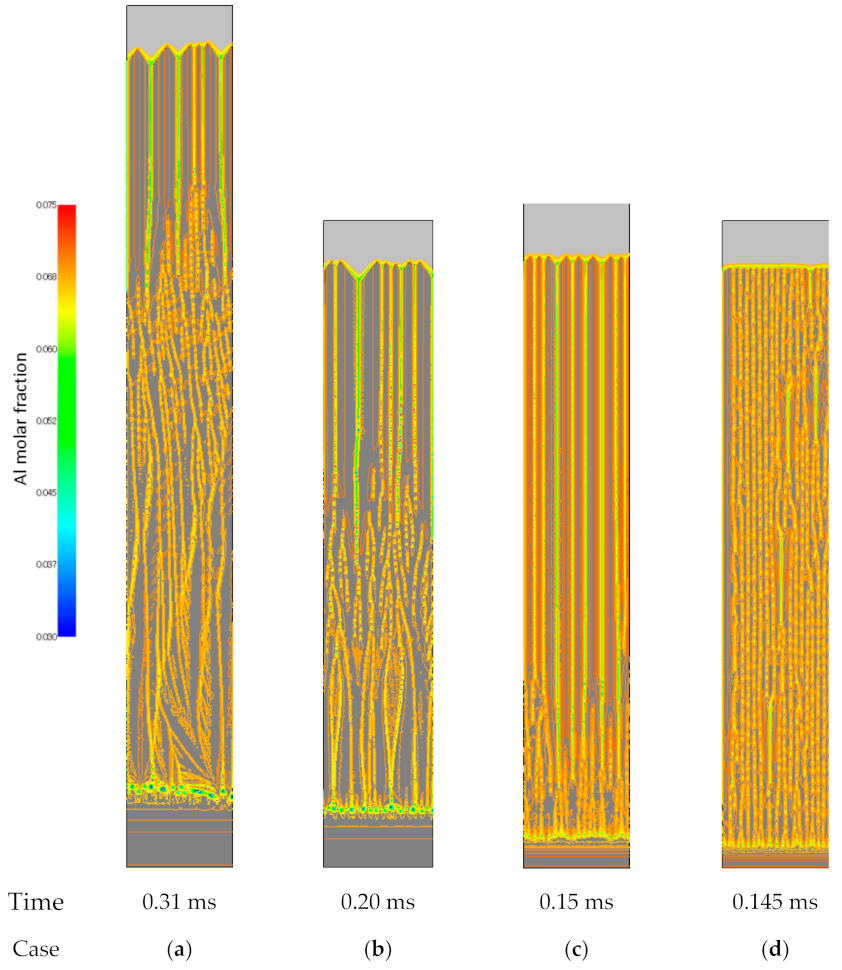
• Columnar solidification microstructure evolutions were performed in cooling rates from 5 × 10⁵ K/s to 1 × 10⁷ K/s at various temperature gradient values while maintaining a constant interface velocity of 0.1 m/s. The results showed that, as the cooling rate increased, the cell space decreased in both equilibrium methods. The average cell space in the non-equilibrium method was larger than that in the quasi-equilibrium method with each cooling rate.
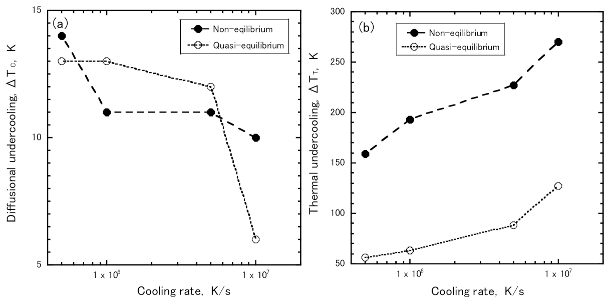
• The thermal undercooling of the non-equilibrium method was much larger than that of the quasi-equilibrium method, whereas the diffusional undercooling was almost the same for both.
• The non-equilibrium MPFM provides us with a more accurate tool for solidification microstructure estimation in LPBF.

References

1. Gorsse, S.; Hutchinson, C.; Gouné, M.; Banerjee, R. Additive manufacturing of metals: A brief review of the characteristic microstructures and properties of steels, Ti-6Al-4V and high-entropy alloys. Sci. Technol. Adv. Mater. 2017, 18, 584–610. [Google Scholar] [CrossRef] [Green Version]
2. Yan, F.; Xiong, W.; Faierson, E.J. Grain structure control of additively manufactured metallic materials. Materials 2017, 10, 1260. [Google Scholar] [CrossRef] [Green Version]
3. Collins, P.C.; Brice, D.A.; Samimi, P.; Ghamarian, I.; Fraser, H.L. Microstructural control of additively manufactured metallic materials. Annu. Rev. Mater. Res. 2016, 46, 63–91. [Google Scholar] [CrossRef]
4. Kok, Y.; Tan, X.P.; Wang, P.; Nai, M.L.S.; Loh, N.H.; Liu, E.; Tor, S.B. Anisotropy and heterogeneity of microstructure and mechanical properties in metal additive manufacturing: A critical review. Mater. Des. 2018, 139, 565–586. [Google Scholar] [CrossRef]
5. Thampy, V.; Fong, A.F.; Calta, N.P.; Wang, J.; Martin, A.A.; Depend, P.J.; Kiss, A.M.; Guss, G.; Xing, Q.; Ott, R.T.; et al. Subsurface cooling rates and microstructural response during laser based metal additive manufacturing. Sci. Rep. 2020, 10. [Google Scholar] [CrossRef]
6. Farshidianfar, M.H.; Khajepour, A.; Gerlich, A.P. Effect of real-time cooling rate on microstructure in Laser Additive Manufacturing. J. Mater. Process. Technol. 2016, 231, 468–478. [Google Scholar] [CrossRef]
7. Scipioni Bertoli, U.S.; Guss, G.; Wu, S.; Matthews, M.J.; Schoenung, J.M. In-situ characterization of laser-powder interaction and cooling rates through high-speed imaging of powder bed fusion additive manufacturing. Mater. Des. 2017, 135, 385–396. [Google Scholar] [CrossRef]
8. Promoppatum, P.; Yao, S.-C.; Pistorius, P.C.; Rollett, A.D.; Coutts, P.J.; Lia, F.; Martukanitz, R. Numerical modeling and experimental validation of thermal history and microstructure for additive manufacturing of an Inconel 718 product. Prog. Addit. Manuf. 2018, 3, 15–32. [Google Scholar] [CrossRef]
9. Shimono, Y.; Oba, M.; Nomoto, S. Solidification simulation of direct energy deposition process by multi-phase field method coupled with thermal analysis. Model. Simul. Mater. Sci. Eng. 2019, 27, 074006. [Google Scholar] [CrossRef] [Green Version]
10. Karayagiz, K.; Elwany, A.; Tapia, G.; Franco, B.; Johnson, L.; Ma, J.; Karaman, I.; Arróyave, R. Numerical and experimental analysis of heat distribution in the laser powder bed fusion of Ti-6Al-4V IISE. Transactions 2019, 51, 136–152. [Google Scholar] [CrossRef]
11. Watari, N.; Ogura, Y.; Yamazaki, N.; Inoue, Y.; Kamitani, K.; Fujiya, Y.; Toyoda, M.; Goya, S.; Watanabe, T. Two-fluid model to simulate metal powder bed fusion additive manufacturing. J. Fluid Sci. Technol. 2018, 13, JFST0010. [Google Scholar] [CrossRef] [Green Version]
12. Song, J.; Chew, Y.; Bi, G.; Yao, X.; Zhang, B.; Bai, J.; Moon, S.K. Numerical and experimental study of laser aided additive manufacturing for melt-pool profile and grain orientation analysis. Mater. Des. 2018, 137, 286–297. [Google Scholar] [CrossRef]
13. Rolchigo, M.R.; Mendoza, M.Y.; Samimi, P.; Brice, D.A.; Martin, B.; Collins, P.C.; LeSar, R. Modeling of ti-W solidification microstructures under additive manufacturing conditions. Metall. Mater. Trans. A 2017, 48, 3606–3622. [Google Scholar] [CrossRef] [Green Version]
14. Lian, Y.; Gan, Z.; Yu, C.; Kats, D.; Liu, W.K.; Wagner, G.J. A cellular automaton finite volume method for microstructure evolution during additive manufacturing. Mater. Des. 2019, 169. [Google Scholar] [CrossRef]
15. Ghosh, S.; McReynolds, K.; Guyer, J.E.; Banerjee, D. Simulation of temperature, stress and microstructure fields during laser deposition of Ti–6Al–4V. Model. Simul. Mater. Sci. Eng. 2018, 26, 075005. [Google Scholar] [CrossRef] [Green Version]
16. Wang, X.; Liu, P.W.; Ji, Y.; Liu, Y.; Horstemeyer, M.H.; Chen, L. Investigation on microsegregation of IN718 alloy during additive manufacturing via integrated phase-field and finite-element modeling. J. Mater. Eng. Perform. 2018, 28, 657–665. [Google Scholar] [CrossRef]
17. Yang, Y.; Kühn, P.; Yi, M.; Egger, H.; Xu, B.-X. Non-isothermal phase-field modeling of heat–melt–microstructure-coupled processes during powder bed fusion. JOM 2020, 72, 1719–1733. [Google Scholar] [CrossRef]
18. Acharya, R.; Sharon, J.A.; Staroselsky, A. Prediction of microstructure in laser powder bed fusion process. Acta Mater. 2017, 124, 360–371. [Google Scholar] [CrossRef]
19. Wu, L.; Zhang, J. Phase field simulation of dendritic solidification of Ti-6Al-4V during additive manufacturing process. JOM 2018, 70, 2392–2399. [Google Scholar] [CrossRef] [Green Version]
20. Boussinot, G.; Apel, M.; Zielinski, J.; Hecht, U.; Schleifenbaum, J.H. Strongly out-of-equilibrium columnar solidification during the Laser Powder-Bed Fusion additive manufacturing process. Phys. Rev. Appl. 2019, 11, 014025. [Google Scholar] [CrossRef] [Green Version]
21. Kitano, H.; Tsuji, M.; Kusano, M.; Yumoto, A.; Watanabe, M. Effect of plastic strain on the solidification cracking of Hastelloy-X in the selective laser melting process. Addit. Manuf. 2021, 37, 101742. [Google Scholar] [CrossRef]
22. Zhang, X.; Chen, H.; Xu, L.; Xu, J.; Ren, X.; Chen, X. Cracking mechanism and susceptibility of laser melting deposited Inconel 738 superalloy. Mater. Des. 2019, 183, 108105. [Google Scholar] [CrossRef]
23. Cloots, M.; Uggowitzer, P.J.; Wegener, K. Investigations on the microstructure and crack formation of IN738LC samples processed by selective laser melting using Gaussian and doughnut profiles. Mater. Des. 2016, 89, 770–784. [Google Scholar] [CrossRef]
24. Ramakrishnan, A.; Dinda, G.P. Direct laser metal deposition of Inconel 738. Mater. Sci. Eng. A 2019, 740–741, 1–13. [Google Scholar] [CrossRef]
25. Steinbach, I.; Zhang, L.; Plapp, M. Phase-field model with finite interface dissipation. Acta Mater. 2012, 60, 2689–2701. [Google Scholar] [CrossRef]
26. Zhang, L.; Steinbach, I. Phase-field model with finite interface dissipation: Extension to multi-component multi-phase alloys. Acta Mater. 2012, 60, 2702–2710. [Google Scholar] [CrossRef]
27. Karayagiz, K.; Johnson, L.; Seede, R.; Attari, V.; Zhang, B.; Huang, X.; Ghosh, S.; Duong, T.; Karaman, I.; Elwany, A.; et al. Finite interface dissipation phase field modeling of Ni–Nb under additive manufacturing conditions. Acta Mater. 2020, 185, 320–339. [Google Scholar] [CrossRef] [Green Version]
28. Kim, S.G.; Kim, W.T.; Suzuki, T. Phase-field model for binary alloys. Phys. Rev. Estat. Phys. Plasmasfluidsand Relat. Interdiscip. Top. 1999, 60, 7186–7197. [Google Scholar] [CrossRef]
29. Zhang, L.; Stratmann, M.; Du, Y.; Sundman, B.; Steinbach, I. Incorporating the CALPHAD sublattice approach of ordering into the phase-field model with finite interface dissipation. Acta Mater. 2015, 88, 156–169. [Google Scholar] [CrossRef]
30. Steinbach, I. Phase-field models in materials science. Model. Simul. Mater. Sci. Eng. 2009, 17, 073001. [Google Scholar] [CrossRef]
31. Nomoto, S.; Wakameda, H.; Segawa, M.; Yamanaka, A.; Koyama, T. Solidification analysis by non-equilibrium phase field model using thermodynamics data estimated by machine learning. Model. Simul. Mater. Sci. Eng. 2019, 27, 084008. [Google Scholar] [CrossRef]
32. Kobayashi, R. Modeling and numerical simulations of dendritic crystal growth. Phys. D 1993, 63, 410–423. [Google Scholar] [CrossRef]
33. Thermodynamics and Properties Software. Available online: https://thermocalc.com/products/thermo-calc/ (accessed on 30 March 2021).
34. Nickel-Based Superalloys Databases. Available online: https://thermocalc.com/products/databases/nickel-based-alloys/ (accessed on 30 March 2021).
35. Short for Thermodynamic Calculation Interface. Available online: https://thermocalc.com/products/software-development-kits/#TQ-Interface (accessed on 30 March 2021).
36. Prasad, A.; Yuan, L.; Lee, P.; Patel, M.; Qiu, D.; Easton, M.; StJohn, D. Towards understanding grain nucleation under Additive Manufacturing solidification conditions. Acta Mater. 2020, 195, 392–403. [Google Scholar] [CrossRef]
37. Kurz, W.; Fisher, D.J. Appendix 6 Thermodynamics of rapid solidification. In Fundamentals of Solidification, 4th ed.; Trans Tech Publications Ltd: Zürich, Switzerland, 1998; pp. 220–225. [Google Scholar]
38. Segawa, M.; Yamanaka, A.; Nomoto, S. Multi-phase-field simulation of cyclic phase transformation in Fe-C-Mn and Fe-C-Mn-Si alloys. Comput. Mater. Sci. 2017, 136, 67–75. [Google Scholar] [CrossRef]
39. Kurz, W.; Fisher, D.J. Chapter four: Solidification microstructure: Cells and dendrite. In Fundamentals of Solidification, 4th ed.; Trans Tech Publications Ltd: Zürich, Switzerland, 1998; pp. 63–88. [Google Scholar]
40. Kusano, M.; Kitano, H.; Watanabe, M. Novel calibration strategy for validation of finite element thermal analysis of selective laser melting process using Bayesian optimization. Addit. Manuf. reviewed.
Figure 1. Solute concentration and γ grain distributions obtained by the non-equilibrium multi-phase field method (MPFM) at 0.06 ms at a cooling rate of 105 K/s. (ah) are Al, C, Co, Cr, Mo, Ta, Ti and W molar fractions, respectively.
Metals 11 00626 g001
Figure 2. Solute concentration and γ grain distributions obtained by the quasi-equilibrium MPFM at 0.06 ms at a cooling rate of 105 K/s. (ah) are Al, C, Co, Cr, Mo, Ta, Ti and W molar fractions, respectively.
Metals 11 00626 g002
Figure 3. Temporal C concentration (molar fraction) and γ grain distributions obtained at a cooling rate of 105 K/s by (a) the non-equilibrium MPFM and (b) the quasi-equilibrium MPFM.
Metals 11 00626 g003
Figure 4. Temporal C concentration (molar fraction) and γ grain distributions obtained at a cooling rate of 107 K/s by (a) the non-equilibrium MPFM and (b) the quasi-equilibrium MPFM.
Metals 11 00626 g004
Figure 5. Temperature variations versus FCC area fraction at various cooling rates (104 K/s, 105 K/s, 106 K/s and 107 K/s) for non- and quasi-equilibrium MPFMs and the Scheil model.
Metals 11 00626 g005
Figure 6. Temperature variation versus FCC area fraction at permeability values of 1 × 10 5   m 3 / J / s , 2 × 10 5   m 3 / J / s and 4 × 10 5   m 3 / J / s at a cooling rate of 107 K/s.
Metals 11 00626 g006
Figure 7. Snapshots of solidification microstructure distributions obtained by the quasi-equilibrium MPFM with Al concentrations (molar fraction) of (a) 5 × 10⁵ K/s and 5 × 10⁶ K/m, (b) 1 × 10⁶ K/s and 1 × 10⁷ K/m, (c) 5 × 10⁶ K/s and 5 × 10⁷ K/m and (d) 1 × 10⁷ K/s and 1 × 10⁸ K/m.
Metals 11 00626 g007
Figure 8. Interface moving velocity with time at (a) 5 × 10⁵ K/s and 5 × 10⁶ K/m, (b) 1 × 10⁶ K/s and 1 × 10⁷ K/m, (c) 5 × 10⁶ K/s and 5 × 10⁷ K/m and (d) 1 × 10⁷ K/s and 1 × 10⁸ K/m, obtained by the quasi-equilibrium MPFM. The red dashed line indicates a steady velocity.
Metals 11 00626 g008
Figure 9. Snapshots of solidification microstructure distributions obtained by the non-equilibrium MPFM at Al concentration (molar fraction) at (a) 5 × 10⁵ K/s and 5 × 10⁶ K/m, (b) 1 × 10⁶ K/s and 1 × 10⁷ K/m, (c) 5 × 10⁶ K/s and 5 × 10⁷ K/m and (d) 1 × 10⁷ K/s and 1 × 10⁸ K/m.
Metals 11 00626 g009
Figure 10. Interface moving velocity with time in case (a): 5 × 10⁵ K/s and 5 × 10⁶ K/m, case (b): 1 × 10⁶ K/s and 1 × 10⁷ K/m, case (c): 5 × 10⁶ K/s and 5 × 10⁷ K/m and case (d): 1 × 10⁷ K/s and 1 × 10⁸ K/m obtained by the non-equilibrium MPFM. The red dashed line indicates the steady velocity.
Metals 11 00626 g010
Figure 11. Schematic illustration of diffusional undercooling, Δ T C , and thermal undercooling, Δ T T , where c 0 is the initial alloy concentration, c l * and T t i p are the liquid concentration and temperature at the tip of the cell, respectively.
Metals 11 00626 g011
Figure 12. Undercooling with cooling rate: (a) diffusional undercooling; (b) thermal undercooling.
Metals 11 00626 g012
Figure 13. Solidified microstructure of Ni(Bal.)-3.2Al-0.1C-8.5Co-16.3Cr-1.65Mo-1.8Ta-3.22Ti-2.7W (wt.%) in the laser powder bed fusion process.
Metals 11 00626 g013