
High-Temperature Oxidation Behaviour of AISI H11 Tool Steel


1
Faculty of Natural Sciences and Engineering, University of Ljubljana, Aškerčeva cesta 12, 1000 Ljubljana, Slovenia
2
Institute of Metals and Technology, Lepi pot 11, 1000 Ljubljana, Slovenia
*
Author to whom correspondence should be addressed.
Metals 2021, 11(5), 758; https://0-doi-org.brum.beds.ac.uk/10.3390/met11050758
Submission received: 20 April 2021
/
Revised: 30 April 2021
/
Accepted: 30 April 2021
/
Published: 4 May 2021
(This article belongs to the Special Issue High-Temperature Behavior of Metals)
Abstract
:The high-temperature oxidation of hot-work tool steel AISI H11 was studied. The high-temperature oxidation was investigated in two conditions, the soft annealed condition, and the hardened and tempered condition. First, calculations of the compositions of the oxide layers formed were carried out using the CALPHAD method. The samples were oxidised in a chamber furnace and in a simultaneous thermal analysis instrument, for 100 h in the temperature range between 400 °C and 700 °C. The first samples were used for metallographic (optical microscopy and scanning electron microscopy) and X-ray diffraction analysis of the formed oxide layers, and the second ones for the analysis of the oxidation kinetics by thermogravimetric analysis. Equations describing the high-temperature oxidation kinetics were derived. The kinetics can be described by three mathematical functions, namely: exponential, parabolic, and cubic. However, which function best describes the kinetics depends on the oxidation temperature and the thermal condition of the steel. Hardened and tempered samples have been shown to oxidise less, resulting in a slower oxidation rate. The oxide layers consist of three sublayers, the inner one being spinel-like oxide (Fe, Cr)3O4, the middle one a mixture of magnetite and hematite and the outer one of hematite. At 700 °C there is also some wüstite in the inner oxide sublayer of the soft annealed sample.
1. Introduction
AISI H11 (1.2343) hot-work tool steel, is a typical representative of the group of chromium hot-work tool steels. It is widely used for the production of tools and dies for high-pressure die casting and forging. The higher concentration of carbide-forming alloying elements improves the high-temperature softening resistance of the steel [1,2]. Since hot-work tool steels usually operate at elevated temperatures, the high-temperature oxidation behaviour of H11 hot-work tool steel is of great importance. Several authors [3,4,5,6,7,8,9] have studied the effect of elevated temperatures on the mechanical and physical properties of hot-work tool steels. With this consideration, we investigate the oxidation kinetics of AISI H11 in the temperature range between 400 °C and 700 °C.
Oxidation is one of the most important types of corrosion. Metals and alloys begin to oxidize in air or other atmospheres containing oxygen [10,11,12,13]. Assuming that oxygen is in the gaseous state, metals (M) are converted to oxides (MaOb), and the reaction proceeds according to the following chemical reaction [12]:
Since the chemical reactions of oxidation are well known, one can calculate the Gibbs free energy of the reactions. The Equation (2) for the Gibbs free energy of reaction (1), is given as [12]:
where μ is the chemical potential, a is the activity, R is the gas constant, p is the pressure and T is the temperature. Assuming that ; and atm (101 325 Pa), Equation (3) can be derived from Equation (2) [12]:
Then the Gibbs free energy for the chemical reaction (1) can be determined [12]:
where K is the equilibrium chemical reaction constant and is the Gibbs free energy change per mole of the reaction at standard conditions. Some of the chemical reactions for the oxidation of metals can be found in the well-known Ellingham diagram [14]. Let us first consider the oxidation of pure metals, it depends on the growth kinetics of the oxide layer, on whether it will protect the metal from oxidizing or not. From a thermodynamic point of view, the chemical reaction (1) proceeds spontaneously from left to right when the total change in Gibbs free energy is negative [10,11,12,13,15].
The oxidation kinetics of metals and alloys can follow several different laws, the most common of which are linear, parabolic, cubic, logarithmic, and inverse logarithmic. In fact, the kinetics is very complex and can also consist of a combination of several laws (linear and parabolic, etc.). The chemical reaction (1) follows a kinetic law that can be described by the following equation [10,11,12,13,15,16,17]:
where ξ is a measure of the extent of the reaction at time t, and n is the number of moles [10,11,12,13,15,16,17]. However, the most common method for studying the oxidation rate is to measure the weight gain of the sample over time. Gravimetry is a particularly suitable method, where the change in weight over time can be measured continuously or discontinuously [17].
Several authors studied high-temperature oxidation of iron in air or pure oxygen atmosphere [11,13,17,18,19,20,21]. The high-temperature oxidation kinetics of iron in the temperature range 700–1250 °C can be expressed by Tammann-type parabolic equation [21]:
where, x is the total thickness of the oxide layer, t is the oxidation time, x0 is the initial thickness of the oxide layer (if some oxides are already present on the surface, otherwise the value is 0) of the parabolic oxidation, and is a constant of the parabolic rate usually given in cm2 s−1. However, since oxidation kinetics are usually studied by a change in mass as a function of oxidation time, a parabolic law can be expressed by the Pilling-Bedworth equation [21,22]:
where W is the change in mass per unit area, due to oxidation of iron, and kp (=) is the parabolic constant in g2 cm−4 s−1, and W0 is the initial mass at the time (t = 0) of parabolic oxidation. In the original Pilling-Bedworth equation [22], W0 is equal to 0. In the considered temperature range, the oxidation follows the parabolic law, the resulting oxide layer consists of a very thin outer sublayer of hematite, a thin intermediate sublayer of magnetite and a thick inner sublayer of wüstite [21,23].
On the other hand, the oxidation of iron below 700 °C is much more complex, so that even the published results of different authors [21,24,25,26,27] are less consistent. In previous studies, it was found that the kinetics of isothermal oxidation of iron in the temperature range (570–700 °C) follows a parabolic law. However, the thicknesses of the individual oxide layers differ from study to study [24,25,26,27].
Regarding the high-temperature oxidation of steels, many studies [21,28,29,30,31,32,33,34,35,36,37] in which the high-temperature oxidation of various steels has been investigated have been carried out. Many ways have been proposed to calculate the rate constant of oxidation kinetics. The most suitable method to obtain the equation to calculate the oxidation rate constant of steel under continuous heating or cooling was developed by Kofstad [38]. According to his interpretation, oxidation following a linear, parabolic, or cubic law can be generally expressed as:
where W is defined as the change in mass per unit area over time t, n is a constant with values of 1, 2, or 3 for the linear, parabolic, or cubic law, and kn is a time-independent rate constant expressed as:
where, B is the constant, T is the absolute temperature, R is the gas constant, and Q is the activation energy. There is also an alternative [39], but since the mass change was measured over time, we used the Kofstad method. Regarding the high-temperature oxidation of hot-work tool steels, there are some studies [40,41,42,43,44] have been carried out. Bidibadi et al. [40] investigated the oxidation behaviour of CrMoV steel, the study sets out the composition of the oxide layers in detail and proves that the inner oxide layer contains spinel-like oxides. Zhang et al. [41] studied the high-temperature oxidation resistance of H13 steel, from the TG curves, there is a mass decrease between 250 °C and 500 °C during the heating, when the oxide layer has already formed, but unfortunately, no further analysis was performed regarding the cause the of mass decrease. On the other hand, Min et al. [42] carried out a prediction and analysis of the oxidation of H13 hot-work tool steel. Using the software Thermo-Calc the compositions of the oxide layers were calculated as a function of oxygen partial pressure, and the oxidation mechanisms in different atmospheres were discussed. Regarding the oxidation of H11 steel, Pieraggi et al. [43] explained the oxidation behaviour of H11 steel in dry and wet air at 600 °C and 700 °C. It was found that the oxidation kinetics follows the parabolic law and is also quite sensitive to the presence of water vapour. Bruckel et al. [44] investigated the isothermal oxidation behaviour of an X38CrMoV5 hot-work tool steel at 600 °C and 700 °C. It was also found that the oxidation kinetics is very sensitive to the presence of water vapour. On the other hand, it was proved that the oxide layer is duplex consisting of an outer hematite sublayer and an inner (Fe, Cr)3O4 sublayer. It was mentioned that carbides could play an important role in the growth process of the oxide layer. These studies served as a first insight into what the formed oxide layers might consist of and how the oxidation kinetics might behave.
2. Materials and Methods
We investigated the H11 (EN X37CrMoV5-1) hot-work tool steel with the chemical composition given in Table 1, measured by wet chemical analysis and infrared absorption after combustion with ELTRA CS-800 (ELTRA GmbH, Haan, Germany).
First the heat treatment of H11 hot-work tool steel was carried out. The austenitization temperature was 1020 °C and the soaking time was 30 min. Quenching was carried out in oil, followed by two-stage tempering, at 550 °C and 620 °C for 2 h, for reaching the hardness 42–44 HRC. The heat treatment was carried out in Bosio EUP-K 6/1200 (Bosio d.o.o., Celje, Slovenia) chamber furnace. Since air atmosphere was used, we had to mill off 2 mm of the steel surface, due to decarburization and oxidation during the heat treatment. Sample preparation using a CNC (Computer Numerical Control) Deckel Maho DMC 63V (Deckel Maho Pfronten GmbH, Pfronten, Germany) machine was next. three different types of samples were prepared, the first ones were cubes with dimensions of 10 mm × 10 mm × 10 mm (length × width × height), which were used during the high-temperature oxidation in the chamber furnace. These samples were specially prepared for further analysis by light optical microscope and SEM (Scanning Electron Microscope). The second set of samples were cuboids with dimensions 10 mm × 10 mm × 5 mm, which were also used during high-temperature oxidation in the chamber furnace. The dimensions are different because the height of the XRD (X-ray Diffraction) sample holder is limited. The last ones are cylinders with dimensions h = 4 mm and Φ = 4 mm, which were used in the high-temperature oxidation in NETZSCH STA (Simultaneous Thermal Analyzer) Jupiter 449C (NETZSCH Holding, Selb, Germany) instrument. All surfaces were polished with 1 μm polycrystalline diamond suspension, after polishing, the samples were ultrasonically cleaned with ethanol and dried on hot air, this procedure was also repeated before each oxidation test.
To get a first insight into the composition of the oxide layers, CALPHAD (CALculation of PHAse Diagrams) simulations were performed with the software Thermo-Calc (Thermo-Calc 2020a, Thermo-Calc Software AB, Stockholm, Sweden) using the thermodynamic database TCOX9 [45] (Metal Oxide Solutions Database). In the diagrams the amount of phase is shown on the Y-axis and the activity of O2 is shown on X-axis. The composition of the oxide sublayers in the formed oxide layer in the studied temperature range (400–700 °C), was calculated. Thermo-Calc software and HSC Chemistry software (HSC Chemistry 9.0, Metso Outotec Finland Oy, Tampere, Finland) were also used to calculate the Gibbs free energy of the oxidation reactions.
High-temperature oxidation was studied at 400 °C, 500 °C, 600 °C, and 700 °C in air atmosphere for 100 h. The samples analysed by light optical microscope, SEM and XRD were oxidised in Bosio EUP-K 6/1200 (Bosio d.o.o., Celje, Slovenia) chamber furnace. The heating rate was 15 °C min−1 and the high-temperature oxidation was carried out in air atmosphere. To improve the oxidation conditions, additional air (79 vol% nitrogen, 21 vol% oxygen 0.9 vol% argon and 0.1 vol% of hydrocarbons and other inert gases) was injected into the furnace at a flow rate of 0.3 L min−1. Cooling was performed in the chamber furnace at the cooling rate of 0.5 C min−1, which was intentionally slow. The main reason was not to damage the oxide layer.
The samples used for the study of kinetics were oxidized in the NETZSCH STA Jupiter 449C (NETZSCH Holding, Selb, Germany) instrument. The heating and cooling rate were 10 °C min−1, in addition air was injected into the furnace at a flow rate of 30 mL min−1 (during the heating/cooling and the isothermal section). Correction runs were also performed prior to sample runs with an empty Al2O3 pedestal on which the samples were located during oxidation. TGA (Thermogravimetric Analysis) was used to study the kinetics.
The samples for SEM analysis were ground and polished. An FEG-SEM (Field Emission Gun Scanning Electron Microscopy) ThermoFisher Scientific Quattro S (ThermoFisher Scientific, Waltham, MA, USA) was used to examine the composition and thickness of the oxide layers. The composition was investigated using EDS (Energy-Dispersive X-ray Spectroscopy) analysis (Ultim® Max, Oxford Instruments, Abingdon, UK). EBSD (Electron Backscatter Diffraction) analysis was also performed using ZEISS CrossBeam 550 (Carl Zeiss AG, Oberkochen, Germany) SEM with HikariSuper EBSD camera (EDAX, Mahwah NJ, USA). In addition, the samples were ground, polished, and etched with Vilella’s reagent for optical microscopy. Microphot FXA, Nikon (Nikon, Minato City, Japan) with 3CCD video camera Hitachi HV-C20A (Hitachi, Ltd., Tokyo, Japan) was used for microstructure analysis. Vickers hardness was measured using Instron Tukon 2100B (Instron, Norwood, MA, USA). The hardness measurements were performed on the metallographically prepared samples (ground and polished), and we only measured the hardness of the steels. PANalytical XPert Pro PW3040/60 (Malvern Panalytical, Malvern, England, UK), X-ray diffractometer with Cu anode (λ = 0.15419 nm) using Bragg-Bretano geometry with a theta-theta goniometer with a radius of 240 mm was used to study the types of oxides in the oxide layers.
Since we were investigating samples in two different conditions soft annealed and hardened and tempered condition, we marked the first ones with H11 (soft annealed) and the second ones with H11-HT (hardened and tempered).
3. Results
3.1. CALPHAD
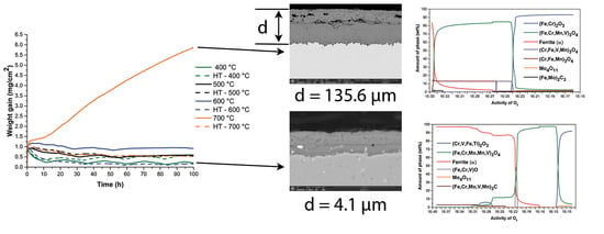
Figure 1 depicts the thermodynamically stable phases in oxide layer and the sublayers formed on the surface of H11 steel at 400 °C (Figure 1a) and 500 °C (Figure 1b). According to this, up to aO ≈ 10−24 (Fe, Cr)2O3 is stable, which predominates (93 wt%), followed by (Fe, Cr, Mn, V)3O4 (3 wt%), Mo4O11 (1.9 wt%), (Cr, Fe, V, Mn)3O4 and (Fe, Mo)2C3 (both together 2.1 wt%). In the range aO ≈ 10−24–10−34, (Fe, Cr, Mn, V)3O4 is predominant (82.8 wt%), followed by (Cr, Fe, V, Mn)3O4 from aO ≈ 10−26 onwards (Cr, Fe, Mn)3O4 (13.1 wt%) and (Fe, Mo)2C3. Ferrite also occurs, increasing with the decreasing aO. At 500 °C there are no drastic changes, all thermodynamically stable phases are the same as at 400 °C, the only difference is the stability of (Fe, Cr)2O3 and (Fe, Cr, Mn, V)3O4, the former is stable from aO ≈ 10−13–10−19 and the latter from aO ≈ 10−19–10−29.
On the other hand, the same changes take place at 600 °C (Figure 2a), (Fe, Cr)2O3 is stable from aO ≈ 10–10–10−15 and (Fe, Cr, Mn, V)3O4 from aO ≈ 10−15–10−25. At both temperatures (500 °C and 600 °C), the calculations also showed that internal oxidation could occur in the steel directly under the oxide layer there could be stable (Fe, Cr, Mn, V)3O4 or (Cr, Fe, Mn, V)3O4. At aO < 10−29 internal oxidation could occur at 500 °C and aO < 10−25 at 600 °C. At 700 °C (Figure 2b), we can see that up to aO ≈ 10–12 (Cr, V, Fe, Ti)2O3 is stable, which is predominant (91.7 wt%), followed by (Fe, Cr, Mo, Mn, V)3O4 (5.4 wt%), Mo4O11 (2.2 wt%) and (Fe, Cr, V) O (0.7 wt%). In the range aO ≈ 10−12–10−22, (Fe, Cr, Mo, Mn, V)3O4 is predominant (97.8 wt%), followed by ferrite, which occurs at aO ≈ 10−16 and increases with decreasing aO (up to aO 10−12–10−22) and then (Fe, Cr, Mo, V, Mn)3C, and Mo4O11 (the content of the latter two together depends on the ferrite content). It is also observed that wüstite appears in the oxide layer and reaches the highest contents at aO ≈ 10−21–10−22, up to 48 wt%. At a temperature of 700 °C, internal oxidation is also present, when aO decreases below 10−22, (Fe, Cr, Mo, Mn, V)3O4 appears just below the surface, and there is also more (Cr, V, Fe, Ti)2O3 present.
3.2. Microscopy
The microstructures after high-temperature oxidation at an individual temperature and the corresponding initial microstructure are shown in Figure 3. It can be seen that the initial microstructure in the soft annealed condition consists of a ferritic (highly decomposed martensite) matrix and spherical carbides. After oxidation at 400 °C, the microstructure consists of a ferrite matrix and spherical carbides. The carbides continue to grow and become even more spherical. After oxidation at 500 °C and 600 °C, the microstructure is very similar to the microstructure obtained after oxidation at 400 °C. There are no significant differences in the microstructure, it consists of a ferrite matrix and spherical carbides. This can also be confirmed by practically equal hardness (Table 2). The drop in hardness, compared to the hardness of the initial condition, is due to the growth of the spheroidized carbides, which become larger and more spherical. This reduces the effect of precipitation hardening. On the other hand, the microstructure of the sample oxidized at 700 °C consists of a ferrite matrix and spherical carbides. The microstructure is very similar to that of the initial sample. This is because this temperature is already in the range of spheroidization annealing.
Figure 4 shows the microstructure after high-temperature oxidation at a single temperature and the corresponding initial microstructural condition. As can be seen from the microstructures, the initial microstructure is in a hardened and tempered state, which means that it consists of martensite and carbides. The microstructure after oxidation at 400 °C and 500 °C remains very similar to the initial microstructure. This indicates that the microstructure is stable in this temperature range. This is also confirmed by the hardness measurements (Table 2), as we see that they change very little, compared to the hardness of the initial state. The microstructure in both cases consists of martensite and carbides. Tempering is the reason that the microstructure is so stable, as the 2nd tempering was at the temperature of 620 °C. After oxidation at a temperature of 600 °C, additional softening occurs, which leads to a drop in hardness (Table 2). The microstructure continues to consist of martensite and carbides. In contrast, after oxidation at a temperature of 700 °C, the microstructure consists of a ferrite matrix and spherical carbides. This is because in this temperature range is already the range of spheroidization annealing.
A thicker oxide layer is formed for the soft annealed samples, except at 600 °C, as evident from the figures showing the oxide layers (Figure 5) and the average of the measured thicknesses (obtained with SEM) of the oxide layers (Table 3). At 400 °C, the oxide layer was 3.9 µm thicker on the soft annealed sample and 1.8 µm thicker at 500 °C, compared to the thickness of the oxide layer on the hardened and tempered samples. On the other hand, the oxide layer formed on the hardened and tempered samples was 3.9 µm thicker at 600 °C. At 700 °C, the oxide layer on the soft annealed sample was thicker again by 22.8 μm.
Carbides are also seen in the microstructures of the soft annealed samples at 400 °C, 500 °C and 600 °C, which are not observed in the hardened and tempered samples because they are finer. The results show the presence of carbides in the inner oxide sublayer, while they are not detected in the outer oxide sublayer. In the soft annealed sample, the oxide layer is solid, and cracking is observed between the inner and middle oxide sublayers. The voids are clearly visible in the oxide layer of the soft annealed samples. They are also believed to form in the oxide layer of the hardened and tempered sample.
The results of EDS analysis of the oxide layer on the soft annealed sample oxidised at 400 °C are shown below (Figure 6a). Since the Fe:O ratio in hematite is 2:3 and the content of other alloying elements is very low compared to the inner oxide sublayer, it can be assumed that the outer oxide sublayer (Figure 6a)—Spectrum 13) consists of hematite. This is followed by two more oxide sublayers. Immediately behind the hematite is magnetite and some hematite (Figure 6a)—Spectrum 14), which form the middle oxide sublayer. Assuming that chromium and silicon are bound in the magnetite and considering the Fe:O ratio in the magnetite (3:4), it can be estimated that the inner oxide sublayer (Figure 6a)—Spectrum 15) is most likely spinel oxide ((Fe, Cr)3O4). In this case, the content of molybdenum, silicon, vanadium, and manganese is also increased, so that the mentioned alloying elements are bound in the spinel. The composition of the steel (Figure 6a)—Spectrum 16) was also analysed, and the matrix near the inner oxide sublayer already has a different chemical composition than the original one. The contents of some alloying elements are higher, these are mainly alloying elements that are also found in the inner oxide sublayer (chromium, molybdenum, and silicon).
The results of EDS analysis of the oxide layer formed on the soft annealed sample oxidised at 500 °C are also shown (Figure 6b). Moreover, in this case, the outer oxide sublayer consists of hematite, which is a bright area on the surface of the oxide layer. The middle oxide sublayer consists of magnetite (Figure 6b)—Spectrum 6). Assuming that chromium and silicon are bound in magnetite and considering the Fe:O ratio in magnetite (3:4), it can be estimated that the inner oxide sublayer (Figure 6b)—Spectrum 7) is most likely spinel oxide ((Fe, Cr)3O4). In this case, the content of molybdenum, silicon, vanadium, and manganese is also increased, so the mentioned alloying elements are most likely bound in the spinel. The composition of the steel (Figure 6b)—Spectrum 8) was also analysed and it was found that the contents of some alloying elements are increased (chromium and nickel), while others are lower (silicon, vanadium, manganese, and molybdenum) compared to the original composition of the steel.
Carbides are observed in the soft annealed sample (Figure 7a), they are finer in the hardened and tempered sample (Figure 7b). The soft annealed sample contains mainly chromium and molybdenum rich carbides and some vanadium carbides. The results show that carbides are also present in the inner and middle sublayer, while they are not observed in the outer oxide sublayer. The concentration of iron is the lowest in the outer sublayer, higher in the inner sublayer and highest in the middle sublayer. On the other hand, the oxygen content is the highest in the outer oxide sublayer and then decreases towards the interior. It can also be seen that there is less chromium in the outer and middle oxide sublayers than in the inner one. Meanwhile, the concentration of molybdenum is greatly increased in the inner sublayer, while it is much lower in the middle and outer oxide sublayers. The nickel content is increased at the contact surface between the oxide layer and the steel. The concentration of silicon is increased in the inner oxide sublayer and then decreases towards the oxide surface.
No major carbides are observed in the hardened and tempered sample (Figure 7b). Moreover, in this case the elements are very homogeneously distributed in the matrix. There are three oxide sublayers and internal oxidation of the steel is also observed i.e., an internal oxidation zone (Figure 7b—IOZ). IOZ occurs just in the case of hardened and tempered sample in the areas where the alloying elements concentrations are increased. The concentration of iron is lowest in the outer oxide sublayer, higher in the inner oxide sublayer and highest in the middle oxide sublayer. On the other hand, the oxygen content is the highest in the outer oxide sublayer and then decreases towards the interior. There are also some areas of increased oxygen content in the steel in the IOZ just below the oxide layer. Chromium concentration is lower in the outer and middle oxide sublayers, than in the inner one. In the case of molybdenum, the concentration is greatly increased in the inner oxide sublayer, compared to the middle and outer. On the other hand, the nickel content is increased at the contact surface between the oxide and the steel. While the silicon content is highest in the inner sublayer, it is slightly lower in the outer and lowest in the middle oxide sublayer.
The oxide layer formed at 700 °C was also investigated by EBSD analysis. First, the areas of the soft annealed sample examined by EBSD analysis are shown (Figure 8). The analysis was divided into four parts, namely: (1) Upper area of oxide layer—outer and part of middle oxide sublayer, (2) Middle area of oxide layer—inner oxide sublayer in contact area with middle oxide sublayer, (3) Middle area of oxide layer—middle area of inner oxide layer and (4) Steel/oxide layer—contact area between steel and inner oxide sublayer.
First, the results for the upper part of the oxide layer are shown (Figure 9). The outer oxide sublayer consists only of hematite. This is followed by a band of magnetite and hematite with low magnetite content, the middle oxide sublayer starts below the magnetite band. The magnetite content in the middle oxide sublayer increases towards the interior. Crystal orientations were coloured with IPF (Inverse Pole Figure) colour coding of orientation maps, IPF-Z standard colour triangle was used.
The inner oxide sublayer (Figure 10) consists mainly of magnetite, together with small amounts of hematite. The composition of magnetite shows an increased concentration of chromium, molybdenum, and silicon. Therefore, along EBSD analysis an EDS analysis of the surface distribution of the elements was also performed. Chromium is distributed throughout the oxide layer (with visible increased concentrations at locations where previously carbides were present), and molybdenum is also concentrated where carbides were most likely previously present. This is already an indication that molybdenum has less influence on the oxidation kinetics than chromium. It can also be seen that a crack forms between the middle and inner oxide sublayers. It is also observed that the chromium content is significantly lower in the middle oxide sublayer. The results show that the inner oxide sublayer is mainly composed of magnetite and some hematite. This indicates that the inner oxide sublayer is very dense, and the magnetite grains are small, resulting in difficult diffusion of both oxygen and iron and other alloying elements.
The analysis of middle area of inner oxide layer (Figure 11) reveals that some wüstite grains are also present, meaning that the inner oxide layer consists of magnetite, some hematite and very little wüstite. An EDS analysis was also performed, examining the concentrations of chromium and molybdenum in the inner oxide sublayer. Distribution is the same as at area (2) middle oxide layer.
The contact area between the oxide layer and the steel (4) was also investigated using EBSD analysis (Figure 12). First, a phase analysis is presented, where it can be observed that a mixed area of magnetite and hematite occurs at the contact area between the inner oxide sublayer and the steel. Carbides are also visible in this area. An analysis of the surface distribution of the elements was also carried out, it shows that the chromium content is increased, and the molybdenum is still present in the places where the carbides were before. This is the indication that molybdenum has less influence on the oxidation kinetics than chromium.
The areas of the hardened and tempered sample examined by EBSD analysis are shown (Figure 13). The analysis was divided into two parts, namely: (1) Upper part of oxide layer—outer and a part of middle oxide sublayer, (2) Middle oxide sublayer—inner oxide sublayer and contact area between steel and inner oxide sublayer.
First, the results for the upper part of the oxide layer are shown (Figure 14). The outer oxide sublayer consists only of hematite. This is followed by a middle oxide sublayer of magnetite and a small amount of hematite, which is stable around the voids and cracks. The cracks between the middle and inner oxide sublayer are also visible.
Meanwhile, the inner oxide sublayer (Figure 15) is mainly magnetite with low hematite content around voids and cracks. There is also a hematite band visible in the oxide layer/steel interface. In this case, no wüstite content was observed. The oxide grains in the inner oxide sublayer are much smaller compared to ones in the soft annealed sample (Figure 10, Figure 11 and Figure 12).
3.3. Thermogravimetric Analysis
Thermogravimetric analysis was used to measure the change in mass of the samples during high-temperature oxidation. The high-temperature oxidation kinetics for the studied steel was described by mathematical functions. An iterative rectangular distance regression algorithm was used for the best fit of the actual curves with the mathematical functions. Equations describing the change in mass of the sample per unit area over time for each experimental temperature are also presented for each sample studied. Since the realistic conditions were simulated, air was blown into the furnace during the heating of the samples in the STA instrument, the curve in the heating segment differs from that under isothermal conditions. Therefore, each oxidation curve is described by two equations, the first giving the oxidation kinetics under heating and the second giving the oxidation kinetics under isothermal conditions. A two-phase and a single-phase exponential growth function (Equations (10) and (11)), a second-degree polynomial (Equation (12)—parabolic law) and a third-degree polynomial (Equation (13)—cubic law) were used to describe the curves.
In all cases, t is the time in s, Δm is the mass change in mg, A is the specific surface area of the sample in cm2, while the other coefficients depend on the temperature and chemical composition of the steel. In cases, where the kinetics can be described by a parabolic or cubic function, the rate constant (kn) was determined. The rate constants were calculated for all the samples studied and for both parts of the curve, after equation (8) was derived using a simple linear regression. The basic equation for calculating the rate constant (kn) is as follows:
where kn is the rate constant, where n can be 1, 2, or 3 in the case of a linear, parabolic, or cubic law, respectively. In the case of the exponential law, 1 < n < 3. The subscript n was named according to the type of equation, so the exponential law has the subscript e, the parabolic p, and the cubic c. It should be added that the results of the rate constant of the first part of the curve are reliable. In the case of the second part, the results are less reliable up to 700 ° C, which can also be seen in the fluctuations of the curves.
Figure 16 shows TG results, the upper graph shows the curves of all the samples studied. It can be seen that the sample in the soft annealed state at 700 °C is different from the others, its final weight gain is 5.91 mg cm−2. Since all the other samples did not gain more than 1.5 mg cm−2 in weight, the scale on the Y-axis was reduced to the 1.5 mg cm−2 in both graphs below (Figure 16b,c). The red rectangle marks the area enlarged in the left graph, where the fluctuations on the curves are visible, which are most pronounced on the curves at 400 °C and 500 °C. The mentioned effect decreases with increasing temperature of oxidation. The blue rectangle marks the area that is enlarged in the graph on the right, where the scale on the X-axis is reduced to 10 h. The reason for this is to show the difference between shape of the curves obtained from the heating section (1st part of the curve) and under isothermal conditions (2nd part of the curve). This will be explained in more detail in the discussion.
Table 4 shows the weight changes in % for the end of each part of the curve are presented. It is obvious that there is a weight loss at isothermal conditions (2nd part) for all the samples studied, except for those soft annealed at 700 °C. This is also evident from the oxidation curves in Figure 16.
Each of the curves (Figure 16) was also described by the mathematical function that best fits the curves of the experimental data. The labels of part 1 (under heating conditions) and part 2 (under isothermal conditions) of the curve are used. It should be noted that oxidation itself under heating conditions affects the kinetics under isothermal conditions. First, the type of equation (Table 5) associated with each part of the curve is presented, and then the corresponding coefficients for each sample studied.
The rate constants k (Table 6) are given for each sample studied and each part of the oxidation curve. In the case of the first part of the curve, the rate constants are accurate and there is not much variation between the results. It can also be determined, from the calculated constants, which sample had the fastest oxidation kinetics when heated, this was clearly H11 (soft annealed) at 700 °C.
However, for the second part they deviate greatly, which is logical as the curves also vary greatly and consequently the linear regression also deviates. However, comparing only the rate coefficients for the second part, a tendency can be seen, most of them are negative, which is the consequence of the mass loss during isothermal oxidation. The fastest oxidation kinetics was found for H11 at 700 °C, which was expected.
3.4. XRD
The results of the XRD analysis of the oxide layers at 400 °C, 500 °C, and 600 °C are shown in Figure 17. They indicate that the layers in both conditions consist of hematite, magnetite, and chromium spinel. Meanwhile, the oxide layer of the soft annealed sample at 700 °C consists of hematite, magnetite, wüstite and chromium spinel. On the other hand, the hardened and tempered sample does not contain wüstite.
4. Discussion
For discussion, we plotted a diagram of Gibbs free energies (Figure 18) for oxidation reactions of some carbides, alloying elements, and oxides, calculated using Thermo-Calc and HSC Chemistry software. All chemical reactions have been normalized to 1 mol O2 for better comparability.
The results of all analyses were used to explain the oxidation kinetics of H11 steel. The oxidation kinetics (Figure 16) is unstable below 700 °C, which can also be seen from the fluctuating oxidation curves. As evidenced by thermodynamic calculations and metallographic analysis, the microstructure of the steel in the soft annealed state consists of a ferrite matrix and spherical carbides (Cr, Mo, Fe)23C6 and VC, and some Ti(C,N). In the case of hardened and tempered state, the microstructure consists of a martensitic matrix and primary (VC and TiCN), and secondary (Cr, Mo, Fe)23C6) carbides. There are more of the latter, as they are precipitated during tempering.
The oxidation kinetics (Figure 16) during heating (Part 1) show in all cases the beginnings of the parabolic or cubic law (best described by the exponential growth function). Under isothermal conditions (part 2), the slope of the curves begins to decrease, except at 700 °C in the case of a soft annealed sample. As can be seen from the results presented, an oxide layer forms during heating and becomes thicker, as the oxidation temperature increases. The weight increases on average from 0.7 mg at 400 °C to 1.1 mg at 700 °C. The reason for this is that oxidation of the matrix and alloying elements and carbides occurs simultaneously during heating. It depends on the formed oxide layer, whether it protects the steel from further oxidation. In other words, whether a formed oxide layer is in thermodynamic equilibrium with the atmosphere under the given conditions or not.
Namely, in the transition from heating to the isothermal part of oxidation, it is crucial, whether the oxide layer is already in thermodynamic equilibrium with the atmosphere and protects the steel from further oxidation or not. The curves decrease at lower temperatures (400–600 °C) and increase at oxidation temperatures of 700 °C in the case of a soft annealed sample. Here it is essential, which has a greater influence on the oxidation rate or which process controls the oxidation kinetics. The oxidation of the iron matrix is on one side and the oxidation of carbides and other alloying elements in the matrix on the other side. In this case, mainly chromium, molybdenum, silicon, and vanadium. At lower temperatures (T < 700 °C), the oxidation of carbides and alloying elements dissolved in the matrix has been shown to have a greater effect on the oxidation kinetics than the oxidation of iron, even though the iron concentration in the matrix is highest. It has been shown that the oxide layer in this temperature range consists of three sublayers, namely the outer hematite, the middle magnetite, and the inner spinel. It is the latter that best protects the steel from further oxidation. Magnetite grows by the predominant transport of Fe2+ cations to wüstite (not yet thermodynamically stable) and Fe3+ to hematite. At the same time, grain boundaries in the oxide layer below 600 °C are very important for diffusion in both magnetite and hematite [12,46,47,48]. However, in this temperature range, diffusion is limited precisely because of the inner oxide sublayer, which consists of spinel oxide, so that the diffusion of iron and oxygen, and thus the growth of the magnetite oxide sublayer is also impeded. This is also contributed by the very fine crystalline grains of magnetite in the inner oxide sublayer (Figure 10, Figure 11 and Figure 12), which further impede diffusion. As a result, oxygen is mainly used for the oxidation of carbides, which are most oxidized at the interface between the middle/inner oxide sublayers. From the calculated Gibbs free energies (Figure 18), chromium should oxidize first, then chromium spinels are formed, afterwards the oxidation of M23C6 carbide starts, followed by the oxidation of iron and finally carbon. The oxidation of the carbides themselves has been reported by several authors [49,50,51,52,53]. It was found that M23C6 carbides start to oxidize in the air atmosphere at elevated temperatures and thus can affect the oxidation kinetics, while MC carbides do not have a much effect on the oxidation kinetics. Recent research [49] has shown that M23C6 (Cr23C6) carbides in high-silicon ferritic/martensitic steel begin to oxidize under isothermal conditions in an atmosphere of air at 823 K. It was found that carbides and areas around (with increased alloying elements) can serve as potential sites for the formation of chromium oxides. In the case of Cr23C6, chromium begins to form chromium oxide (Cr2O3), which is a product of carbide oxidation. At the same time, the oxidation of the carbide itself also produces CO2 [51], which is also a product of oxidation, the chemical reaction proceeds as follows:
The remaining molybdenum, silicon and iron also diffuse into the spinel oxide and partially into the magnetite. However, chromium, will not form a single oxide (Cr2O3), due to its low chromium content (5% by weight) [49,54,55]. As a result, it will react with iron and oxygen after a chemical reaction (16) to form a spinel-shaped oxide that forms the inner oxide sublayer.
At the same time, MC (VC) carbides themselves do not have a significant effect on the oxidation kinetics because, as can be seen from the Gibbs free energy calculations (Figure 18), they oxidize last, slowly decompose into the inner oxide sublayer during oxidation, vanadium slowly diffuses into spinel oxides due to the decomposition of carbides and increases the density of the inner oxide sublayer. At the same time, it has been demonstrated [35,49] that silicon is also incorporated into the spinel oxide.
There are more causes of curve oscillations (Figure 16). As can be seen from the chemical reaction (15) and the oxidation reactions of other carbides (Figure 18), CO2 is the product of carbide oxidation. This means that the local gas volume in the inner oxide sublayer will increase, especially at the interface with the middle sublayer, as carbide oxidation is most intense there. At the same time, the expansion coefficients (α) of the individual oxides formed must be considered. The CO2 formed during the oxidation of carbides will leave the oxide layer, which is seen on the curve as a slope in the negative direction, as at the same time stresses are created in the oxide layer, causing cracking, and some oxide to fall off. It has been proven by other authors that if the resulting gas (CO or CO2, as in our case) cannot escape through micro channels (micro pores and cracks), its pressure begins to increase, leading to the formation of new pores or even cracking or oxide layer fractures [21,56]. Mainly for the purpose of demonstrating that part of the oxide layer is crumbling, we also took an image of the morphology of the oxide layer (Figure 19—orange circles) with a SEM to explain the oscillations of the curves obtained with TG.
At high-temperature oxidation at 700 °C, the aforementioned effect is still visible in a hardened and tempered sample, but in the soft annealed condition, it is only visible at the beginning of the oxidation, after which the oxidation rate depends mainly on oxygen and iron diffusion. This means that there is a faster diffusion of oxygen and iron in the soft annealed sample, and the resulting inner oxide sublayer and carbide oxidation no longer control the oxidation kinetics. In this case, chromium rich M23C6 carbides are no longer oxidized as intensively, but begin to decompose and thus the alloying elements begin to diffuse into the magnetite and form an inner oxide sublayer as is the case with other carbides. This can also be seen by the fact that both the inner and middle oxide sublayers are thicker than those that form in the temperature range between 400 °C and 600 °C. In addition, wüstite begins to form in the inner oxide sublayer, where iron diffusion is most rapid. In the hardened and tempered sample, the influence of carbide oxidation is still present, which is also evident from the curves. The curves at about 55 h oxidation slowly begin to flatten their shape (no oscillations are visible), indicating that the oxidation of the carbides no longer controls the oxidation kinetics.
In the soft annealed samples, the oxide grows throughout the crystal grain and on the carbides. In a hardened and tempered sample, the areas with increased contents of alloying elements and carbides oxidize first and then the matrix begins to oxidize.
Regarding the composition of the oxide layer, in all cases the oxide layer has the same composition and differs only in the thicknesses, which increase with temperature. Thus, the oxide layer consists of three sublayers, namely the outer hematite, the middle magnetite and the inner one of spinel oxide (Fe, Cr)3O4. At the oxidation temperature of 700 °C in the case of the soft annealed sample, the inner oxide sublayer consists of spinel and some wüstite. However, in the case of the hardened and tempered sample, no wüstite was detected. At the same time, a hematite band also appears on the contact surface between the steel and the inner oxide sublayer at the temperature of 700 °C. A similar composition of the oxide layer has also been reported by other researchers [40,57,58]. The thicknesses increase from 3.8 μm to 154.2 μm for the soft annealed sample and from 0.1 μm to 117.1 μm for the hardened and tempered sample (Table 3).
In the temperature range 400–600 °C, the oxide layer also consists of three sublayers (Figure 5). The inner oxide sublayer consists of spinel oxide ((Fe, Cr)3O4), which also contains increased concentrations of molybdenum, silicon, vanadium, and manganese. The middle oxide sublayer is also composed of magnetite, in which the concentrations of chromium, molybdenum, silicon, manganese and vanadium are much lower. The outer oxide sublayer, which is very thin, consists of hematite. This is also consistent with thermodynamic calculations, except in the case of molybdenum oxide, which was not formed. Thermodynamic calculations also indicated that internal oxidation should take place, which can be confirmed only in the case of the hardened and tempered sample, namely after oxidation at the temperature of 600 °C. Figure 20 shows the oxide layer of the H11 hot-work tool steel in soft annealed state, after oxidation at 500 °C. There are no differences in the composition of the oxide layer between soft annealed and hardened and tempered samples up to 700 °C. The only difference is the density of the inner oxide sublayer, which is denser in the hardened and tempered samples, as shown by the EBSD results.
At 700 °C (Figure 21) in the case of the soft annealed state, the outer oxide sublayer also consists of hematite, the middle of magnetite and some hematite, and the inner of magnetite (Fe, Cr)3O4, hematite bands, and some wüstite. On the other hand, the oxide layer formed on the hardened and tempered sample after oxidation at a temperature of 700 °C was denser and did not contain any wüstite, as shown by the results of the EBSD analysis (Figure 15).
The morphology of the oxide layer formed in soft annealed (H11) and hardened and tempered (H11-HT) samples after oxidation at a temperature of 400 °C is shown in Figure 22. In the case of the soft annealed sample, the oxide starts to grow over the entire surface. On the other hand, in the case of the hardened and tempered sample, the areas with elevated concentrations of alloying elements and carbides begin to oxidize first.
5. Conclusions
Chemical composition affects high-temperature oxidation. It depends on the alloying elements, their content and affinity for oxygen, whether they form independent oxides or whether they are involved in oxidation processes at all. In the case of AISI H11 hot-work tool steel, silicon has the greatest affinity to oxygen, followed by chromium, molybdenum, carbon, and others. However, silicon did not have much influence on the high-temperature oxidation, since it was not present in the carbides (only in the matrix) and on the other hand soft annealed samples had faster oxidation kinetics. So, we assumed that chromium is the element that starts to oxidize first, since it was also present in the carbides.
Carbides and areas around (with increased concentration of alloying elements) can serve as potential sites for the formation of oxides. This is most evident at lower temperatures 400–500 °C, where oxidation of the Cr23C6 carbides controls the oxidation kinetics. Oxidation of the carbides causes stresses in the inner oxide sublayer, leading to pores and cracks, but can also lead to crumbling of the oxide layer, which is most evident in the oxidation kinetics at 400 °C. The higher the temperature, the smaller the effect, as diffusion is already so rapid that oxidation of the carbides no longer affects the oxidation kinetics of the steel, so that even Cr23C6 carbides (≥700 °C) begin to slowly dissolve into the inner oxide sublayer at higher temperatures. Other carbides present, however, have no significant influence on oxidation.
The oxide layers formed during heating are in some cases sufficient protection to preserve the steel from further oxidation. The result is that the mass, which has increased during heating remains almost unchanged during further oxidation under isothermal conditions. This is observed at a temperature of 500 °C, and even more so at a temperature of 600 °C for both samples (soft annealed and hardened and tempered). Similarly, for the hardened and tempered sample at a temperature of 700 °C. In these cases, the change in mass is minimal, confirming the assumption that an oxide layer formed during heating provides sufficient protection to keep the steel from further oxidation.
Oxidation kinetics are also affected by the heat treatment of the steel. In general, the oxidation kinetics of the hardened and tempered samples are slower than the oxidation kinetics of the soft annealed samples. Small differences occur at a temperature of 400 °C and 500 °C. However, at 600 °C and 700 °C a difference is seen between soft annealed and hardened and tempered samples, with the oxidation kinetics of the latter being slower. This is largely influenced by the alloying elements dissolved in the matrix. More alloying elements are dissolved in the hardened and tempered samples and consequently the inner oxide sublayer formed is denser, preventing further diffusion of iron and oxygen.
Heat treatment affects the growth of the oxide layer and the size of the crystal grains in the oxide layer. As has been shown, the oxide layer, especially the inner sublayer, is denser in hardened and tempered samples. As a result, the growth of the oxide layer is slower because the diffusion of oxygen, iron and other alloying elements is impeded. Consequently, since the crystal grains in the matrix of the hardened and tempered samples are much smaller, the crystal grains in the oxide layer, especially in the inner sublayer, are also smaller than in the soft annealed samples.
Thermodynamic calculations give a first insight into the composition of the oxide layer. From the calculated thermodynamic results, one can conclude which oxides will form after oxidation at a given temperature. It has been shown that the calculations can be very accurate, provided we set all the input data correctly.
Author Contributions
Conceptualization and writing, T.B.; original draft preparation, T.B., J.B., M.V.; methodology and formal analysis, T.B., J.B., J.M., B.Š.B., M.V.; validation and formal analysis, T.B., J.B., B.Š.B., M.V.; supervision, J.M. and M.V. All authors have read and agreed to the published version of the manuscript.
Funding
Funding was provided by the Slovenian Research Agency ARRS program P2-0344 (B) and P2-0050 (C).
Data Availability Statement
Not applicable.
Conflicts of Interest
The authors declare no conflict of interest.
References
- Mesquita, R.A. Tool steels: Properties and performance; CRC Press: Boca Raton, FL, USA, 2016. [Google Scholar]
- Roberts, G.; Krauss, G.; Kennedy, R. Tool Steels, 5th ed.; ASM International: Materials park, OH, USA, 1998. [Google Scholar]
- Zhou, Q.; Wu, X.; Shi, N.; Li, J.; Min, N. Microstructure evolution and kinetic analysis of DM hot-work die steels during tempering. Mater. Sci. Eng. A 2011, 528, 5696–5700. [Google Scholar] [CrossRef]
- Medvedeva, A.; Bergström, J.; Gunnarsson, S.; Andersson, J. High-temperature properties and microstructural stability of hot-work tool steels. Mater. Sci. Eng. A 2009, 523, 39–46. [Google Scholar] [CrossRef]
- Zhang, Z.; Delagnes, D.; Bernhart, G. Microstructure evolution of hot-work tool steels during tempering and definition of a kinetic law based on hardness measurements. Mater. Sci. Eng. A 2004, 380, 222–230. [Google Scholar] [CrossRef] [Green Version]
- Mebarki, N.; Delagnes, D.; Lamesle, P.; Delmas, F.; Levaillant, C. Relationship between microstructure and mechanical properties of a 5% Cr tempered martensitic tool steel. Mater. Sci. Eng. A 2004, 387–389, 171–175. [Google Scholar] [CrossRef] [Green Version]
- Jilg, A.; Seifert, T. Temperature dependent cyclic mechanical properties of a hot work steel after time and temperature dependent softening. Mater. Sci. Eng. A 2018, 721, 96–102. [Google Scholar] [CrossRef]
- Caliskanoglu, D.; Siller, I.; Ebner, R.; Leitner, H.; Jeglitsch, F.; Waldhauser, W. Thermal Fatigue and Softening Behavior of Hot Work Tool Steels. Proc. 6th Int. Tool. Conf. 2002, 2, 707–719. [Google Scholar]
- Markežič, R.; Mole, N.; Naglič, I.; Šturm, R. Time and temperature dependent softening of H11 hot-work tool steel and definition of an anisothermal tempering kinetic model. Mater. Today Commun. 2020, 22. [Google Scholar] [CrossRef]
- Lai, G.Y. High-Temperature Corrosion And Materials Applications; ASM International: Materials park, OH, USA, 2007. [Google Scholar]
- Revie, R.W. Uhlig’s corrosion handbook; John Wiley & Sons, Inc.: Hoboken, NJ, USA, 2011. [Google Scholar]
- Richardson, T.J.A.; Cottis, B.; Lindsay, R.; Lyon, S.; Scantlebury, D.; Stott, H.; Graham, M. Shreir’s Corrosion; Elsevier Science: London, UK, 2009; Volume 1. [Google Scholar]
- Cramer, S.D.; Covino Jr, B.S. ASM Handbook Volume 13B: Corrosion: Materials; ASM International: Materials Park, OH, USA, 2005; Volume 13. [Google Scholar]
- Ellingham, H.J.T. Reducibility of oxides and sulphides in metallurgical processes. J. Soc. Chem. Ind. 1944, 63, 125–160. [Google Scholar] [CrossRef]
- Popov, B.N. Corrosion Engineering: Principles and Solved Problems; Elsevier: London, UK, 2015. [Google Scholar]
- Pedeferri, P. Corrosion Science and Engineering; Springer International Publishing: Cham, Switzerland, 2018. [Google Scholar]
- Young, D.J. High Temperature Oxidation and Corrosion of Metals; Elsevier: London, UK, 2008. [Google Scholar]
- Birks, N.; Meier, G.H.; Pettit, F.S. Introduction to the High Temperature Oxidation of Metals; Cambridge University Press: Cambridge, UK, 2006. [Google Scholar]
- Hauffe, K. Oxidation of metals; Springer US: New York, NY, USA, 1965. [Google Scholar]
- Davies, M.H.; Simnad, M.T.; Birchenall, C.E. On the Mechanism and Kinetics of the Scaling of Iron. JOM 1951, 3, 889–896. [Google Scholar] [CrossRef]
- Chen, R.Y.; Yeun, W.Y.D. Review of the High-Temperature Oxidation of Iron and Carbon Steels in Air or Oxygen. Oxid. Met. 2003, 59, 433–468. [Google Scholar] [CrossRef]
- Pilling, N.B.; Bedworth, R.E. Oxidation of metals at high temperatures. J. Inst. Met. 1923, 29, 529–539. [Google Scholar]
- Ajersch, F. Scale formation in steel processing operation. In Proceedings of the 34th Mechanical Working and Steel Processing Conference Proceedings; KUHN, L.G., Ed.; Iron and Steel Society: Warrendale, PA, USA, 1993; pp. 419–437. [Google Scholar]
- Caplan, D.; Cohen, M. Effect of cold work on the oxidation of iron from 400–650 °C. Corros. Sci. 1966, 6, 327–335. [Google Scholar] [CrossRef]
- Caplan, D.; Sproule, G.I.; Hussey, R.J. Comparison of the kinetics ofhigh-temperature oxidation of Fe as influenced by metal purity and cold work. Corros. Sci. 1970, 10, 9–17. [Google Scholar] [CrossRef]
- Caplan, D.; Cohen, M. Scaling of iron at 500 °C. Corros. Sci. 1963, 3, 139–143. [Google Scholar] [CrossRef]
- Boggs, W.E.; Kachik, R.H. The Oxidation of Iron-Carbon Alloys at 500 °C. J. Electrochem. Soc. 1969, 116, 424–430. [Google Scholar] [CrossRef]
- Abuluwefa, H.; Guthrie, R.I.L.; Ajersch, F. The effect of oxygen concentration on the oxidation of low-carbon steel in the temperature range 1000 to 1250 °C. Oxid. Met. 1996, 46, 423–440. [Google Scholar] [CrossRef]
- Chen, R.Y.; Yuen, W.Y. Oxidation of low-carbon, low-silicon mild steel at 450–900 °C under conditions relevant to hot-strip processing. Oxid. Met. 2002, 57, 53–79. [Google Scholar] [CrossRef]
- Caplan, D.; Sproule, G.I.; Hussey, R.J.; Graham, M.J. Oxidation of Fe-C alloys at 500 °C. Oxid. Met. 1978, 12, 67–82. [Google Scholar] [CrossRef]
- Caplan, D.; Sproule, G.I.; Hussey, R.J.; Graham, M.J. Oxidation of Fe-C alloys at 700 °C. Oxid. Met. 1979, 13, 255–272. [Google Scholar] [CrossRef]
- Malik, A.U.; Whittle, D.P. Oxidation of Fe-C alloys in the temperature range 600–850 °C. Oxid. Met. 1981, 16, 339–353. [Google Scholar] [CrossRef] [Green Version]
- Cao, G.; Liu, X.; Sun, B.; Liu, Z. Morphology of oxide scale and oxidation kinetics of low carbon steel. J. Iron Steel Res. Int. 2014, 21, 335–341. [Google Scholar] [CrossRef]
- Bak, S.-H.; Kim, M.-J.; Lee, J.-H.; Bong, S.-J.; Kim, S.-K.; Lee, D.-B. High-temperature oxidation kinetics and scales formed on Fe-2.3%Cr-1.6%W alloy. J. Korean Ceram. Soc. 2011, 48, 57–62. [Google Scholar] [CrossRef]
- Hao, M.; Sun, B.; Wang, H. High-Temperature Oxidation Behavior of Fe–1Cr–0.2Si Steel. Materials 2020, 13, 509. [Google Scholar] [CrossRef] [Green Version]
- Li, D.; Dai, Q.; Cheng, X.; Wang, R.; Huang, Y. High-Temperature Oxidation Resistance of Austenitic Stainless Steel Cr18Ni11Cu3Al3MnNb. J. Iron Steel Res. Int. 2012, 19, 74–78. [Google Scholar] [CrossRef]
- Ghosh, S.; Kumar, M.K.; Kain, V. High temperature oxidation behavior of AISI 304L stainless steel - Effect of surface working operations. Appl. Surf. Sci. 2013, 264, 312–319. [Google Scholar] [CrossRef]
- Kofstad, P. Oxidation of Metals: Determination of Activation Energies. Nature 1957, 179, 1362–1363. [Google Scholar] [CrossRef]
- Browne, K.M.; Dryden, J.; Assefpour, M. Modelling Scaling and Descaling in Hot Strip Mills. In Proceedings of the Recent Advances in Heat Transfer and Micro-Structure Modelling for Metal Processing; Too, J.J.M., Guo, R.-M., Eds.; American Society of Mechanical Engineers: San Francisco, CA, USA, 1995; pp. 187–198. [Google Scholar]
- Bidabadi, M.H.S.; Chandra-ambhorn, S.; Rehman, A.; Zheng, Y.; Zhang, C.; Chen, H.; Yang, Z.G. Carbon depositions within the oxide scale and its effect on the oxidation behavior of low alloy steel in low (0.1 MPa), sub-(5 MPa) and supercritical (10 MPa) CO2 at 550 °C. Corros. Sci. 2020, 177, 108950. [Google Scholar] [CrossRef]
- Zhang, X.; Jie, X.; Zhang, L.; Lui, S.; Zheng, Q. Improving the high-temperature oxidation resistance of H13 steel by laser cladding with a WC/Co-Cr alloy coating. Anti-Corrosion Methods Mater. 2016, 63, 171–176. [Google Scholar] [CrossRef]
- Min, Y.; Wu, X.; Wang, K.; Li, L.; Xu, L. Prediction and analysis on oxidation of H13 hot work steel. J. Iron Steel Res. Int. 2006, 13, 44–49. [Google Scholar] [CrossRef]
- Pieraggi, B.; Rolland, C.; Bruckel, P. Morphological characteristics of oxide scales grown on H11 steel oxidised in dry or wet air. Mater. High Temp. 2005, 22, 61–68. [Google Scholar] [CrossRef]
- Bruckel, P.; Lamesle, P.; Lours, P.; Pieraggi, B. Isothermal oxidation behaviour of a hot-work tool steel. Mater. Sci. Forum. 2004, 461, 831–838. [Google Scholar] [CrossRef]
- Thermo-Calc Software. TCOX9 - TCS Metal Oxide Solutions Database, 7. Database version 9; Thermo-Calc Software: Solna, Sweden, 1992. [Google Scholar]
- Atkinson, A. Transport processes during the growth of oxide films at elevated temperature. Rev. Mod. Phys. 1985, 57, 437–470. [Google Scholar] [CrossRef]
- Atkinson, A.; Taylor, R.I. Diffusion of 55Fe in Fe2O3 single crystals. J. Phys. Chem. Solids 1985, 46, 469–475. [Google Scholar] [CrossRef]
- Channing, D.A.; Graham, M.J. A study of iron oxidation processes by Mössbauer spectroscopy. Corros. Sci. 1972, 12, 271–280. [Google Scholar] [CrossRef]
- Ye, Z.; Wang, P.; Li, D.; Li, Y. M23C6 precipitates induced inhomogeneous distribution of silicon in the oxide formed on a high-silicon ferritic/martensitic steel. Scr. Mater. 2015, 97, 45–48. [Google Scholar] [CrossRef]
- Gong, Y.; Young, D.J.; Kontis, P.; Chiu, Y.L.; Larsson, H.; Shin, A.; Pearson, J.M.; Moody, M.P.; Reed, R.C. On the breakaway oxidation of Fe9Cr1Mo steel in high pressure CO2. Acta Mater. 2017, 130, 361–374. [Google Scholar] [CrossRef]
- Jung, K.H.; Kim, S.J. Role of M23C6 carbide on the corrosion characteristics of modified 9Cr-1Mo steel in N2-O2-CO2-SO2 atmosphere at 650 °C. Appl. Surf. Sci. 2019, 483, 417–424. [Google Scholar] [CrossRef]
- Wu, S.; Fei, Y.; Guo, B.; Jing, L. Corrosion of Cr23C6 coated Q235 steel in wet atmospheres containing Na2SO4 at 750 °C. Corros. Sci. 2015, 100, 306–310. [Google Scholar] [CrossRef]
- Li, Z.; Cao, G.; Lin, F.; Cui, C.; Wang, H.; Liu, Z. Phase transformation behavior of oxide scale on plain carbon steel containing 0.4 wt.% Cr during continuous cooling. ISIJ Int. 2018, 58, 2338–2347. [Google Scholar] [CrossRef] [Green Version]
- Mrowec, S. On the mechanism of high temperature oxidation of metals and alloys. Corros. Sci. 1967, 7, 563–578. [Google Scholar] [CrossRef]
- Wood, G.C. High-temperature oxidation of alloys. Oxid. Met. 1970, 2, 11–57. [Google Scholar] [CrossRef]
- Sachs, K.; Brown, J.R. A theory of decarburization by scale. J. Iron Steel Inst. 1958, 190, 169–170. [Google Scholar]
- Saunders, S.R.J.; Monteiro, M.; Rizzo, F. The oxidation behaviour of metals and alloys at high temperatures in atmospheres containing water vapour: A review. Prog. Mater. Sci. 2008, 53, 775–837. [Google Scholar] [CrossRef]
- Zurek, J.; Wessel, E.; Niewolak, L.; Schmitz, F.; Kern, T.U.; Singheiser, L.; Quadakkers, W.J. Anomalous temperature dependence of oxidation kinetics during steam oxidation of ferritic steels in the temperature range 550–650 °C. Corros. Sci. 2004, 46, 2301–2317. [Google Scholar] [CrossRef]
Figure 1.
Amount of thermodynamically stable phases formed during high-temperature oxidation as a function of oxygen activity for H11 steel at (a) 400 °C and (b) 500 °C.
Figure 1.
Amount of thermodynamically stable phases formed during high-temperature oxidation as a function of oxygen activity for H11 steel at (a) 400 °C and (b) 500 °C.

Figure 2.
Amount of thermodynamically stable phases formed during high-temperature oxidation as a function of oxygen activity for H11 steel at (a) 600 °C and (b) 700 °C.
Figure 2.
Amount of thermodynamically stable phases formed during high-temperature oxidation as a function of oxygen activity for H11 steel at (a) 600 °C and (b) 700 °C.

Figure 3.
Etched microstructure of H11 hot-work tool steel in the soft annealed state in initial state and after oxidation at 400 °C, 500 °C, 600 °C and 700 °C for 100 h.
Figure 3.
Etched microstructure of H11 hot-work tool steel in the soft annealed state in initial state and after oxidation at 400 °C, 500 °C, 600 °C and 700 °C for 100 h.

Figure 4.
Etched microstructure of H11 hot-work tool steel in the hardened and tempered state in initial state and after oxidation at 400 °C, 500 °C, 600 °C and 700 °C for 100 h.
Figure 4.
Etched microstructure of H11 hot-work tool steel in the hardened and tempered state in initial state and after oxidation at 400 °C, 500 °C, 600 °C and 700 °C for 100 h.

Figure 5.
H11 hot-work tool steel in soft annealed and hardened and tempered state and oxide layer formed after high-temperature oxidation at 400 °C, 500 °C, 600 °C and 700 °C.
Figure 5.
H11 hot-work tool steel in soft annealed and hardened and tempered state and oxide layer formed after high-temperature oxidation at 400 °C, 500 °C, 600 °C and 700 °C.

Figure 6.
The areas analysed with EDS are shown with the corresponding chemical composition in at% for oxide layers and wt% for steel. Results are shown for samples in the soft annealed state after high-temperature oxidation at (a) 400 °C and (b) 500 °C.
Figure 6.
The areas analysed with EDS are shown with the corresponding chemical composition in at% for oxide layers and wt% for steel. Results are shown for samples in the soft annealed state after high-temperature oxidation at (a) 400 °C and (b) 500 °C.

Figure 7.
EDS element mapping images are shown for samples in the (a) soft annealed and (b) hardened and tempered state after high-temperature oxidation at 600 °C.
Figure 7.
EDS element mapping images are shown for samples in the (a) soft annealed and (b) hardened and tempered state after high-temperature oxidation at 600 °C.

Figure 8.
Areas of the oxide layer of the soft annealed sample after high-temperature oxidation at 700 °C analysed by EBSD analysis.
Figure 8.
Areas of the oxide layer of the soft annealed sample after high-temperature oxidation at 700 °C analysed by EBSD analysis.

Figure 9.
EBSD analysis of the oxide layer of the soft annealed sample after high-temperature oxidation at 700 °C (1) Upper part of the oxide layer—outer and part of the middle oxide sublayer.
Figure 9.
EBSD analysis of the oxide layer of the soft annealed sample after high-temperature oxidation at 700 °C (1) Upper part of the oxide layer—outer and part of the middle oxide sublayer.

Figure 10.
EBSD analysis of the oxide layer of the soft annealed sample after high-temperature oxidation at 700 °C (2) Middle oxide layer—inner oxide sublayer in contact area with middle oxide sublayer.
Figure 10.
EBSD analysis of the oxide layer of the soft annealed sample after high-temperature oxidation at 700 °C (2) Middle oxide layer—inner oxide sublayer in contact area with middle oxide sublayer.

Figure 11.
EBSD analysis of the oxide layer of the soft annealed sample after high-temperature oxidation at 700 °C (3) Middle oxide layer—middle area of inner oxide layer.
Figure 11.
EBSD analysis of the oxide layer of the soft annealed sample after high-temperature oxidation at 700 °C (3) Middle oxide layer—middle area of inner oxide layer.

Figure 12.
EBSD analysis of the oxide layer of the soft annealed sample after high-temperature oxidation at 700 °C (4) Steel/oxide layer—contact area between steel and inner oxide sublayer.
Figure 12.
EBSD analysis of the oxide layer of the soft annealed sample after high-temperature oxidation at 700 °C (4) Steel/oxide layer—contact area between steel and inner oxide sublayer.

Figure 13.
Areas of the oxide layer of the tempered and hardened sample after high-temperature oxidation at 700 °C analysed by EBSD analysis.
Figure 13.
Areas of the oxide layer of the tempered and hardened sample after high-temperature oxidation at 700 °C analysed by EBSD analysis.

Figure 14.
EBSD analysis of the oxide layer of the hardened and tempered sample after high-temperature oxidation at 700 °C (1) Upper part of oxide layer—outer and a part of middle oxide sublayer.
Figure 14.
EBSD analysis of the oxide layer of the hardened and tempered sample after high-temperature oxidation at 700 °C (1) Upper part of oxide layer—outer and a part of middle oxide sublayer.

Figure 15.
EBSD analysis of the oxide layer of the hardened and tempered sample after high-temperature oxidation at 700 °C (2) Middle oxide sublayer—inner oxide sublayer and contact area between steel and inner oxide sublayer.
Figure 15.
EBSD analysis of the oxide layer of the hardened and tempered sample after high-temperature oxidation at 700 °C (2) Middle oxide sublayer—inner oxide sublayer and contact area between steel and inner oxide sublayer.

Figure 16.
TG results for all the investigated samples of H11 hot-work tool steel (a) TG results, (b) enlarged Y-axis to the 1.5 mg cm−2 and (c) enlarged X-axis to the 10 h and Y-axis to the 1.5 mg cm−2.
Figure 16.
TG results for all the investigated samples of H11 hot-work tool steel (a) TG results, (b) enlarged Y-axis to the 1.5 mg cm−2 and (c) enlarged X-axis to the 10 h and Y-axis to the 1.5 mg cm−2.

Figure 17.
Results of XRD analysis of all samples examined.

Figure 18.
Calculated Gibbs free energies for oxidation reactions of selected carbides, alloying elements, and oxides.
Figure 18.
Calculated Gibbs free energies for oxidation reactions of selected carbides, alloying elements, and oxides.

Figure 19.
Oxide layer morphology for H11 steel after oxidation at 400 °C. The places where the oxide has fallen off (orange circles) and where the oxide has formed on the carbide (red squares) are marked.
Figure 19.
Oxide layer morphology for H11 steel after oxidation at 400 °C. The places where the oxide has fallen off (orange circles) and where the oxide has formed on the carbide (red squares) are marked.

Figure 20.
Oxide layer of H11 steel in the soft annealed state after oxidation at a temperature of 500 °C.
Figure 20.
Oxide layer of H11 steel in the soft annealed state after oxidation at a temperature of 500 °C.

Figure 21.
Oxide layer of H11 steel in the soft annealed state after oxidation at a temperature of 700 °C.
Figure 21.
Oxide layer of H11 steel in the soft annealed state after oxidation at a temperature of 700 °C.

Figure 22.
Morphology of the oxide layer of the soft annealed (H11) and hardened and tempered (H11-HT) sample after oxidation at a temperature of 400 °C.
Figure 22.
Morphology of the oxide layer of the soft annealed (H11) and hardened and tempered (H11-HT) sample after oxidation at a temperature of 400 °C.


Table 1.
Chemical composition of investigated H11 hot-work tool steel given in weight percent.
| Sample | C | Si | Mn | P | S | Cr | Ni | Mo | V | Fe |
|---|---|---|---|---|---|---|---|---|---|---|
| H11 | 0.36 | 0.97 | 0.54 | 0.015 | 0.002 | 5.05 | 0.09 | 1.22 | 0.38 | Bal. |
Table 2.
Measured hardness of H11 hot-work tool steel in soft annealed (H11) and hardened and tempered (H11-HT) state before and after oxidation.
Table 2.
Measured hardness of H11 hot-work tool steel in soft annealed (H11) and hardened and tempered (H11-HT) state before and after oxidation.
| Sample | Hardness [HV 10] | ||||
|---|---|---|---|---|---|
| Before Oxidation | After Oxidation | ||||
| 400 °C | 500 °C | 600 °C | 700 °C | ||
| H11 | 180 | 166 | 163 | 164 | 164 |
| H11-HT | 478 | 460 | 466 | 294 | 243 |
Table 3.
Thickness of the oxide layer formed on H11 hot-work tool steel in the soft annealed (H11) and hardened and tempered (H11-HT) state after high-temperature oxidation at 400 °C, 500 °C, 600 °C and 700 °C.
Table 3.
Thickness of the oxide layer formed on H11 hot-work tool steel in the soft annealed (H11) and hardened and tempered (H11-HT) state after high-temperature oxidation at 400 °C, 500 °C, 600 °C and 700 °C.
| Temperature [°C] | Thickness of Oxide Layer [µm] | |
|---|---|---|
| H11 | H11-HT | |
| 400 | 4.1 | 0.2 |
| 500 | 6.5 | 4.7 |
| 600 | 10.9 | 14.8 |
| 700 | 135.6 | 112.8 |
Table 4.
The weight changes in % for each part of the curve.
| Temperature [°C] | Part of the Curve | TG [%] | |
|---|---|---|---|
| H11 | H11-HT | ||
| 400 | 1. | 0.168 | 0.175 |
| 2. | 0.038 | 0.095 | |
| 500 | 1. | 0.183 | 0.184 |
| 2. | 0.113 | 0.109 | |
| 600 | 1. | 0.218 | 0.191 |
| 2. | 0.178 | 0.034 | |
| 700 | 1. | 0.242 | 0.223 |
| 2. | 1.138 | 0.101 | |
Table 5.
The coefficients are given for each part of the oxidation curve the studied samples with the corresponding equation type.
Table 5.
The coefficients are given for each part of the oxidation curve the studied samples with the corresponding equation type.
| Temperature [°C] | Sample | Part of Curve | Equation Type | Number of the Equation | Coefficients | ||||
|---|---|---|---|---|---|---|---|---|---|
| A | B | C | D | E | |||||
| 400 | H11 | 1. | exponential | 10 | −0.44 | −192.54 | −0.58 | −1432.74 | 0.99 |
| 2. | exponential | 10 | 0.70 | −9660.25 | 0.16 | −230,346.79 | 0.17 | ||
| H11 HT | 1. | exponential | 10 | −0.44 | −200.67 | −0.64 | −1502.7 | 1.04 | |
| 2. | exponential | 11 | 0.70 | −6444.01 | / | / | 0.46 | ||
| 500 | H11 | 1. | exponential | 10 | −0.48 | −217.16 | −0.64 | −1948.81 | 1.09 |
| 2. | cubic | 13 | 0.94 | −5.73∙10−6 | 2.41∙10−11 | −3.03∙10−17 | / | ||
| H11 HT | 1. | exponential | 10 | −0.52 | −220.61 | −0.67 | −2415.19 | 1.14 | |
| 2. | cubic | 13 | 0.99 | −4.10∙10−6 | 1.00∙10−11 | −5.22∙10−18 | / | ||
| 600 | H11 | 1. | exponential | 10 | −0.48 | −193.42 | −0.94 | −2639.44 | 1.38 |
| 2. | cubic | 13 | 1.25 | −4.61∙10−6 | 1.92∙10−11 | −2.42∙10−17 | / | ||
| H11 HT | 1. | exponential | 10 | −0.41 | −242.47 | −0.62 | −2181.65 | 1.12 | |
| 2. | exponential | 10 | 0.56 | −11,080.79 | 0.49 | −54,103.34 | 0.13 | ||
| 700 | H11 | 1. | exponential | 10 | −0.42 | −185.2 | −0.81 | −1759.68 | 1.27 |
| 2. | parabolic | 12 | 1.03 | 1.62∙10−5 | −6.89∙10−12 | / | / | ||
| H11 HT | 1. | exponential | 10 | −0.41 | −186.54 | −0.73 | −1490.03 | 1.16 | |
| 2. | exponential | 11 | 0.58 | −56,349.86 | / | / | 0.54 | ||
Number of the equation: A two-phase exponential (10), a single-phase exponential (11), a second-degree polynomial (12—parabolic law) and a third-degree polynomial (13—cubic law).
Table 6.
The rate constants are given for each part of the oxidation curve for the studied samples with the corresponding equation type.
Table 6.
The rate constants are given for each part of the oxidation curve for the studied samples with the corresponding equation type.
| Temperature [°C] | Sample | Part of Curve | Equation Type | Rate Constants | ||
|---|---|---|---|---|---|---|
| ke [mge cm−2e s−1] | kp [mg2 cm−4 s−1] | kc [mg3 cm−6 s−1] | ||||
| 400 | H11 | 1. | exponential | 3.104∙10−4 | / | |
| 2. | exponential | −2.650∙10−7 | / | |||
| H11 HT | 1. | exponential | 3.475∙10−4 | / | ||
| 2. | exponential | 9.300∙10−8 | / | |||
| 500 | H11 | 1. | exponential | 2.998∙10−4 | / | / |
| 2. | cubic | / | / | −1.700∙10−7 | ||
| H11 HT | 1. | exponential | 2.936∙10−4 | / | / | |
| 2. | cubic | / | / | −1.57∙10−6 | ||
| 600 | H11 | 1. | exponential | 4.089∙10−4 | / | / |
| 2. | cubic | / | / | −1.134∙10−7 | ||
| H11 HT | 1. | exponential | 2.770∙10−4 | / | / | |
| 2. | exponential | −4.983∙10−7 | / | / | ||
| 700 | H11 | 1. | exponential | 4.983∙10−4 | / | / |
| 2. | parabolic | / | 7.744∙10−5 | / | ||
| H11 HT | 1. | exponential | 4.487∙10−4 | / | / | |
| 2. | exponential | −1.526∙10−6 | / | / | ||
Publisher’s Note: MDPI stays neutral with regard to jurisdictional claims in published maps and institutional affiliations. |
© 2021 by the authors. Licensee MDPI, Basel, Switzerland. This article is an open access article distributed under the terms and conditions of the Creative Commons Attribution (CC BY) license (https://creativecommons.org/licenses/by/4.0/).
Share and Cite
MDPI and ACS Style
Balaško, T.; Vončina, M.; Burja, J.; Šetina Batič, B.; Medved, J. High-Temperature Oxidation Behaviour of AISI H11 Tool Steel. Metals 2021, 11, 758. https://0-doi-org.brum.beds.ac.uk/10.3390/met11050758
AMA Style
Balaško T, Vončina M, Burja J, Šetina Batič B, Medved J. High-Temperature Oxidation Behaviour of AISI H11 Tool Steel. Metals. 2021; 11(5):758. https://0-doi-org.brum.beds.ac.uk/10.3390/met11050758
Chicago/Turabian StyleBalaško, Tilen, Maja Vončina, Jaka Burja, Barbara Šetina Batič, and Jožef Medved. 2021. "High-Temperature Oxidation Behaviour of AISI H11 Tool Steel" Metals 11, no. 5: 758. https://0-doi-org.brum.beds.ac.uk/10.3390/met11050758
Note that from the first issue of 2016, this journal uses article numbers instead of page numbers. See further details here.