
Industrial X-ray Image Analysis with Deep Neural Networks Robust to Unexpected Input Data


1
Department of Engineering Science, University West, SE-461 86 Trollhättan, Sweden
2
Department of Electrical Engineering, Chalmers University, SE-412 96 Göteborg, Sweden
*
Author to whom correspondence should be addressed.
Metals 2022, 12(11), 1963; https://0-doi-org.brum.beds.ac.uk/10.3390/met12111963
Submission received: 29 September 2022
/
Revised: 28 October 2022
/
Accepted: 10 November 2022
/
Published: 16 November 2022
(This article belongs to the Special Issue Modern Non-destructive Testing for Metallic Materials)
Abstract
:X-ray inspection is often an essential part of quality control within quality critical manufacturing industries. Within such industries, X-ray image interpretation is resource intensive and typically conducted by humans. An increased level of automatization would be preferable, and recent advances in artificial intelligence (e.g., deep learning) have been proposed as solutions. However, typically, such solutions are overconfident when subjected to new data far from the training data, so-called out-of-distribution (OOD) data; we claim that safe automatic interpretation of industrial X-ray images, as part of quality control of critical products, requires a robust confidence estimation with respect to OOD data. We explored if such a confidence estimation, an OOD detector, can be achieved by explicit modeling of the training data distribution, and the accepted images. For this, we derived an autoencoder model trained unsupervised on a public dataset with X-ray images of metal fusion welds and synthetic data. We explicitly demonstrate the dangers with a conventional supervised learning-based approach and compare it to the OOD detector. We achieve true positive rates of around at false positive rates of around on samples similar to the training data and correctly detect some example OOD data.
1. Introduction
Non-destructive evaluation (NDE) is an integral part of quality control within many quality-concerned manufacturing industries, e.g., aerospace and energy. An NDE method commonly utilized is X-ray inspection, and for high-value and critical products typically all of the material volume, e.g., all welded material, on all of the product individuals is inspected. Thus, a high level of automatization of X-ray inspection is desirable.
Industrial X-ray inspection can be divided into three steps: planning, data sampling, and data interpretation. The automatization of the interpretation is one of the bottlenecks for quality-critical industries. With interpretation, we mean the operation of transforming (mainly) the X-ray image data into information that can be utilized later for decisions, e.g., decisions regarding the material quality. The interpretation is typically done with extensive amounts of manual labor.
Most of the automatic industrial X-ray image interpretation algorithms in literature have some steps in common: pre-processing, segmentation, feature extraction, and classification. The preprocessing step typically includes image data calibration, noise removal, and contrast enhancement. In some cases, the background noise, e.g., the weld geometry, is subtracted with reference radiographs [1], polynomial weld geometry approximations [2], or low pass filters [3]. Contrast enhancement operations, with, e.g., histogram equalization, is also common [1].
For the segmentation step, many methods have been studied over the years. A comprehensive comparative study on segmentation methods for metal fusion-weld defect segmentation can be found in [4]. The study confirmed trends in other studies, where edge detection-based segmentations are typically optimal for crack-like defects, region-growing are optimal for cavity-like defects, and watershed-based segmentation for the lack-of-fusion and similar defects.
Feature extraction, where each segmented region is described by a feature vector in a suitable space and classification can be done with manually designed feature extractors or automatically as in, e.g., deep learning (DL) [5]. The cases of manually derived features, followed by a supervised classifier, have been extensively studied for the application of metal fusion welds and aluminum castings, some examples are: fuzzy logic systems combined with geometrical features ([6], accuracy ) and contrast-variance features ([7], accuracy ); support vectors machines (SVM) with geometrical and texture features ([8], accuracy ); artificial neural networks (ANN) with geometrical features ([9], accuracy ), texture/geometrical features ([10], accuracy ); and random forest classifiers with Haar-like features ([11], accuracy ). Studies on unsupervised classification are few, but in a recent study on weld defect classification, a high accuracy of around was reached [12] utilizing shape features and a generalized Gaussian mixture model. Overall the studies indicate high accuracies when tested on data similar to the training data. Moreover, there is a tendency for simple features, related to local variation, to perform well, such as in [11] (welds), which utilized Haar-like features, and in [13] (aluminum castings), where local binary pattern features [14] give the best results.
The DL approach was also explored for the analysis of industrial X-ray images. In [15,16], features were derived unsupervised with an autoencoder, and then utilized for supervised training of a weld defect classifier (accuracy ). Pixel-level segmentation of weld defects (utilizing a fully convolutional deep neural network similar to UNet [17] and trained with a supervised approach) was demonstrated in [18]. Another model also similar to the Unet architecture was explored in [19], in the X-ray images of welds but from another dataset. Moreover, in [20], a deep neural network was successfully trained for weld defect classification (accuracy ). Moreover, aluminum casting inspections have been explored with DL. In [21], a deep convolutional neural network was trained–supervised to classify whether or not image patches contained material defects. Moreover, in [22], the segmentations of industrial X-ray computed tomography 3D data were successfully explored with a UNet-similar model trained on modeled data.
In parallel to the above-described approach with segmentation, feature extraction, and supervised classification, there are also studies on more statistical hypothesis testing or residual analysis approaches, where anomalies, with respect to an accepted (material defect-free) training dataset, are identified in test images. A model is derived for the accepted intensity variation, and the residual image (the original input minus modeled) is analyzed [23,24,25]. A test statistic is calculated for the residual image, often within local small regions, and deviations are identified as anomalous or not with respect to the expected noise. Sophisticated more complex statistical models and sparse reconstructions or dictionary learning [26] for the accepted variation have also been explored. Studies on such sparse models have indicated both promising results ([27] and accuracy of for welds), as well as some discouraging ([13], accuracy of for aluminum casting data). Recently, DL-based approaches have started to attract attention, such as in [28] (the authors focused on industrial X-ray CT data) and industrial X-ray inspections of die-casts in [29]; both utilized autoencoders to detect anomalies in X-ray images.
In summary, many of the earlier studies showed promising results with high accuracies on test data similar to training data. However, very few [28,29] of the studies have explicitly addressed how the algorithms react when subjected to unexpected new input data far from the training distribution, so-called out-of-distribution (OOD) data. In principle, dictionary learning and sparse coding should be able to detect OOD data, though there has been very limited explicit exploration. We claim that a confidence estimation (with respect to OOD data) is important and should be addressed, and we argue for this by referring to NDE reliability and the emerging NDE 4.0 [30] (NDE in the fourth industrial revolution).
The problem is related to the NDE reliability field. The field is divided into questions dealing with reproducibility (e.g., calibration), repeatability (e.g., stable process), and capability (e.g., probability of detection, POD) [31]. The POD [32], a well-established concept, is a statistical measure of the largest defect that will not be detected. Given a large number of parameters (e.g., specific material, component geometry, manufacturing process, material defects, flaw populations, and so on), each with their statistical distribution, the POD can be derived as a function of, e.g., the specific material flaw size. The POD is typically specific to a particular inspection case and requires that the above-listed parameter distributions do not change without control. A well-calibrated–stable-repeatable inspection, with quantified capability, is essential for a reliable NDE.
We strongly believe there will always be the risk of unexpected OOD data arriving at the NDE interpretation step in some of the cases, indicating low-quality products (and some not). We further suspect that a population of human operators will currently excel over data-based computer algorithm interpreters in reasonably dealing with such OOD data. The human capability of critically thinking with concrete knowledge outside of the training data set, e.g., involving material and manufacturing process understanding, will bring clarity to how to interpret OOD data. At the same time, the repetitive mundane tasks of interpreting inspection data very similar to the training data (in most cases, defect-free material) can be processed—to a high degree of accuracy—by the computer algorithms.
Human factors also impact the NDE reliability. Models for deriving, POD which include understanding the human factors, have been proposed, as in the X-ray inspection case in [33,34], where the detectability of defects (with respect to the human observer’s vision system capabilities) was addressed. More complex human factors influencing the reliability have also been addressed. In [35], the risks and challenges with mechanized NDT were studied from the viewpoint of human factors, e.g., it was concluded that redundancy in humans, instructed to monitor automatic algorithms, did not necessarily improve the reliability. Simply letting the human operators review all of the machine interpretations will not solve the safety issues, and certainly not the resource efficiency problem.
As we proceed into the fourth industrial revolution (Industry 4.0), NDE is predicted to also change [30]. In a recent article [36], the concept of intelligence augmentation in NDE was elaborated on. Human intelligence enhanced by artificial intelligence, rather than AI working alone, was proposed as a possibility for NDE for Industry 4.0. Our current study connects to this, as we propose that an integral part of such enhanced human intelligence involves the capability of the computer algorithm to correctly estimate confidence, especially with respect to OOD input, which is still an open scientific question. With a confidence estimate, with respect to OOD data, new input, far from the training data distribution, can be identified by the computer algorithm, such as low confidence in interpretations, and be delivered to a human for further processing; at the same time, most of the data, i.e., the parts similar to the training data can be interpreted safely by computer algorithms alone.
In this work, we focused on how to achieve a robust confidence estimation with respect to OOD data, when interpreting industrial X-ray images. Essentially, it can be seen as an OOD detector algorithm. We propose (and experimentally explored) a solution based on utilizing a deep learning autoencoder-based convolutional neural network model for modeling the accepted variation in the input image. The model was trained unsupervised in a denoising mode, with an additional perturbation dataset containing material defects and synthetic indications representing non-accepted variations in input images.
Our approach has conceptual similarities with the above-mentioned sparse representation and statistical hypothesis approaches, i.e., it models accepted variations in input images. Moreover, as in [28,29], we utilized deep learning-based autoencoders that were trained unsupervised to model the accepted X-ray intensity distributions, as opposed to most of the earlier studies, which also utilized autoencoders, but only for deriving features later used for supervising the learning of a classifier. To the best of our knowledge, our approach to modeling the accepted variations in input with autoencoders trained unsupervised with such perturbation datasets of structural noise, together with the localized kernel loss term, is new within X-ray imaging analyses.
This work is based on one of our previously published conference papers and can be considered an extended version of [37]. The unsupervised model and its description are essentially the same (as well as the state-of-the-art and the background). However, in this current work, we expanded the conference paper and explicitly compared the unsupervised–trained model to a supervised–trained binary classifier (deep convolutional neural network), as well as trained and tested the algorithms in a more systematic way (e.g., utilizing synthetic data) than in [37]. In this current study, we successfully show (a) the dangers with supervised–trained deep learning classifiers, with respect to unexpected data and the application area industrial X-ray inspection; (b) that the performance (true positive rate at a fixed false positive rate) of the unsupervised–trained OOD detector was comparable to or better than a supervised–trained classifier on a dataset of X-ray images of metal fusion welds; (c) that synthetic data can be utilized to increase the performance of the unsupervised–trained OOD detector.
2. Background
For the OOD detector, we propose a framework that models the actual pixel intensities of the training dataset. The modeled intensities are then subtracted from the input to form a reconstruction error image, e.g., a residual image. Large deviations in the reconstruction image will flag the existence of OOD data, something unexpected, an anomaly; that is, the residual image intensity distribution will be related to a level of confidence with respect to OOD data. The concept is similar to [23,24,25]. However, those previous studies used other models to model the pixel intensities.
The proposed OOD detector can be trained unsupervised to model material with accepted quality (e.g., accepted welds) or trained with known defects, or a set of different models can be trained on each of them separately, with each separating the intensity variations originating from different higher abstraction level entities, such as weld geometries and different material defects. Optionally, a conventional classifier-trained–supervised model can be utilized to further split the dataset into classes. We suggest that additional information refinement, such as quantifying the size of material defects, should be related to existing international standards, e.g., the quality levels of imperfections in fusion-welded joints are defined in ISO 5817; ISO 17636-2 defines how to perform X-ray inspections of metal fusion welds.
This current work explores the proposed OOD detector concept via modeling of the accepted metal fusion welding geometry utilizing an autoencoder (AE) deep learning model. Further information refinement is not addressed here. This is why we refer to the anomalies, defects, and material imperfections or flaws as one class; the criticality of the anomaly (flaw or defect, accepted or not accepted with respect to the required quality) is not addressed in this model (in order to simplify this work). Moreover, only defect or anomaly indications reasonably detectable by humans with the current inspection setup were considered, i.e., other NDE methods or other X-ray setup suitabilities for the application were also out of the scope of this study.
For an introduction to deep learning see [5]. In brief, AE models are trained to reconstruct the input, by transforming the input into a latent space representation (code or z-space) with an encoder, and then reconstructing the input from the latent space with a decoder. AE models have previously been successfully utilized to discover patterns in input data, in the feature selection for classification, denoising, and so on.
The concept to utilize deep learning models for anomaly detection has already been explored for various applications, such as computer vision and medical imaging. Reference [38], regarding the computer vision field, where an AE was trained on accepted input images and anomalies were identified in the reconstructed error images, is very similar to what we conducted in this work. Other approaches to the confidence estimation of results from deep neural networks, e.g., drop-out approximation of the Bayesian inference, as in [39], and ensemble approaches, as in [40], are interesting; however, as pointed out in [38], they likely do not address the problem with test data far from the training data.
Early and important work on anomaly detection with deep learning models can be found within the medical imaging field. In [41], an AE was trained unsupervised on the image data of optical tomography imaged healthy tissue. Potentially unhealthy tissue (anomalies) were successfully detected by comparing the test image z-space coordinates to a modeled (one-class support vector machine [42]) z-space distribution of healthy tissue.
A similar optical imaging dataset was utilized in [43] to explore an anomaly detection approach with a deep generative adversarial network (GAN) [44]. A GAN was trained to generate new data similar to the data it was trained on; in an adversarial training setup, a discriminator model was trained to discern between real and generated data while competing against a generator model trained to fool the discriminator. Promising results were reported in [43] regarding identifying anomalies with the trained discriminator part of the GAN as well as the reconstruction errors. The model was improved in [45], with fast mapping from the input image space to the z-space (not part of GANs).
Within medical X-ray imaging, similar ideas on anomaly detection have been explored. In [46], abnormal chest tissue was successfully identified with an adversarial AE model trained on X-ray images of healthy tissue. They added skip-connections in the AE, similar to the UNet architecture [17], in order to better preserve high-frequency content in the reconstructed image.
Anomaly detection in airport security screening X-ray images is another studied application area. In [47], an adversarially trained AE model was derived with an additional encoder after the encoder–decoder part of the AE. The authors claimed the additional encoder enabled the modeling of the normal/accepted image z-space distribution. Promising results on detecting anomalies by comparing the test image z-space coordinates to the training data distribution in z-space were shown.
In this work, we explored an approach to AE modeling not based on adversarial training. Instead, we added a localized maximum deviation reconstruction loss term, and trained the model on both accepted input images as well as on systematic noise from non-accepted (anomalies) images. The systematic noise images were added in order to delimit the generalization capabilities of the AE in order to address the problem with high similarity between the accepted and non-accepted images within our selected application of industrial X-ray inspection of metal fusion welds. The systematic noise consisted of real experimental anomalies as well as synthetic ones.
Our proposed approach applied to industrial X-ray inspection has already been addressed in the conference paper [37], of which, this current work, as noted, is an expansion. We also explored the approach to X-ray computed tomography data in [48]. Recently, a similar approach was also explored in [28] on industrial X-ray CT data and on industrial X-ray inspection of die-casts in [29]. However, in [28], the analysis of the residual image was conducted with a neural network binary classifier rather, as opposed to our case (see Section 3.1), with mean and standard deviations in localized kernels. Moreover, in both [28,29], the AE was not trained with anomalies as systematic noise (no perturbation dataset) or localized kernel loss terms, as in our case (see Section 3.1). To the best of our knowledge, our explored approach to OOD detection on X-ray-based images, with an unsupervised training, a perturbation dataset with highly structural noise, and localized loss kernels, was not explored earlier.
3. Materials and Methods
In this section, the models and datasets utilized are described. First, the proposed OOD detector is described, consisting of an autoencoder trained unsupervised and a residual analysis model based on the X-ray imaging noise distribution. Second, the binary classifier trained–supervised (a convolutional neural network) is described. Finally, the datasets, real experimental as well as synthetic, are described in detail.
3.1. OOD Detector Model
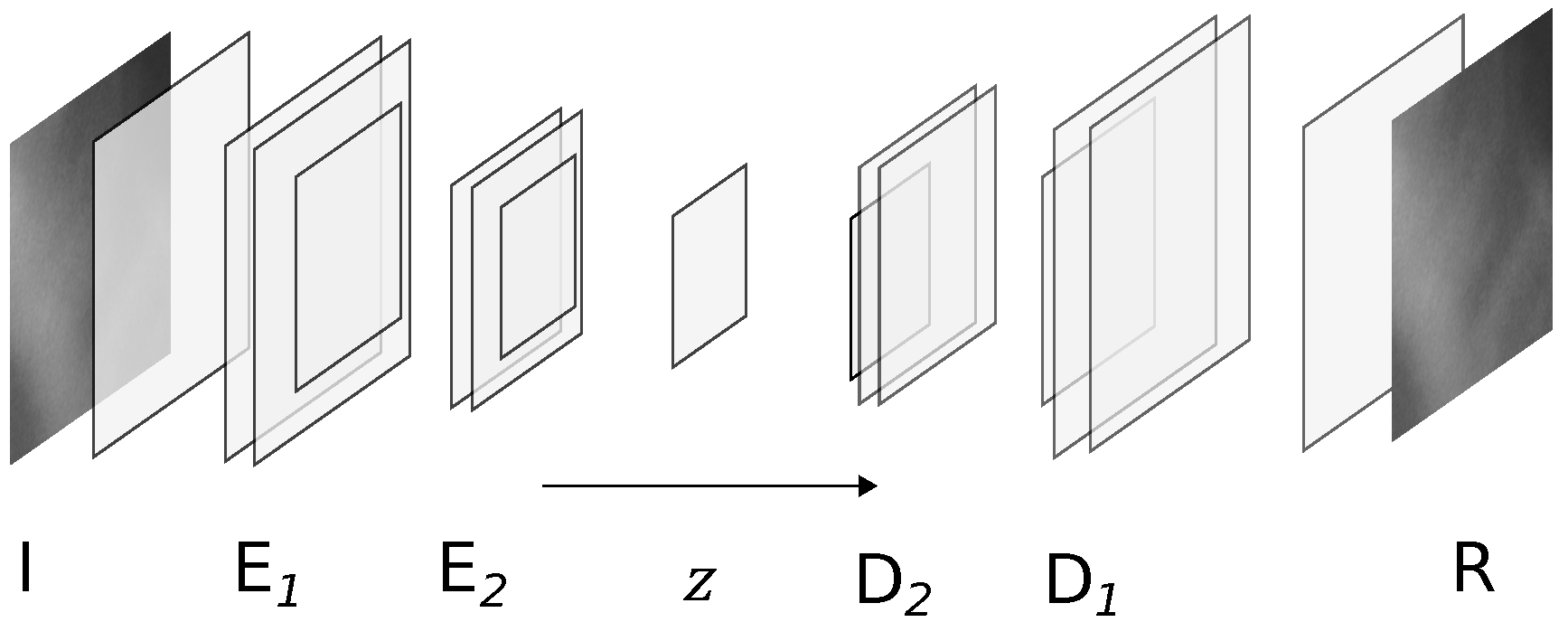
The first part of the OOD detector model is the autoencoder (AE) model utilized for modeling the accepted X-ray intensity variations in the X-ray images. The AE model architecture is outlined in Figure 1. The input image (I) is first encoded by the encoder blocks into the latent space z and then decoded by the decoder blocks () into its reconstruction image (R). The encoder blocks each consist of two 2D convolution layers, separated by a dropout layer, and are followed by a single down-scaling 2D convolution layer with a stride of two pixels. The down-scaling was conducted with the strided convolution layer [49] instead of a max or average pooling layer since it improved the performance for this specific architecture. The number of convolution filters in each convolution layer was 18 for convolution layers in block 1 and 24 for layers in block 2.
The latent space z, preceded by a 2D convolution layer with a filter depth of one, has a ReLU (rectified linear unit) activation with a value bound to the interval . In addition, sparsity of the latent space is promoted with a L1 regularizer, which was implemented by adding a loss term . The L1 scaling was kept small, in order to keep the importance of the regularization low compared to the other loss terms (specified below).
The decoder (D) is made symmetric to the encoder, with the same number of convolution filters as the encoder. Each decoder block consists of a dropout layer (dropout fraction ), a transposed 2D convolution layer with a stride of two pixels (up-sampling), and two 2D convolution layers. The reconstructed image (R) is preceded by a single filter 2D convolution layer.
Overall, all convolution layers have small kernels of size as well as, unless otherwise noted, ReLU activations. Moreover, to make the model intrinsically bound to the reconstruction of an as-limited input variation as possible (ideally only the accepted patches), it was kept small, with a total of about 41,000 trainable parameters and a small z-space.
The input image patch size was fixed at . The resulting dimension was and the reconstructed image (R) region (aperture) was .
The AE model architecture is almost identical to the one derived in [37]. The differences are that this current model has two 2D convolutions in series in each block and only two blocks in the encoder/decoder, instead of one 2D convolution in each block and three blocks in the encoder/decoder, as in [37].
Some of the X-ray image intensity variation in the accepted/okay weld patches are very similar to the intensity variation (e.g., in shape and size) in the not accepted/defect-containing weld patches. Industrial X-ray image interpretation is not trivial (partly due to the radiographic noise level). Therefore, the AE model could typically easily be undesirably trained to reconstruct unseen defect-containing patches to a high precision.
It was shown in [37] that this problem could be mitigated by setting up the model and training simultaneously to identify a compressed z-space high information density data representation (representation learner), as well as a denoising filter. In the denoising part, noise consisting of real and synthetic material defect indications was added during training and forced to not be reconstructed by the AE model. The hypothesis was that these two approaches would yield a highly compact AE model, optimized only for reconstructing images similar to the accepted weld patches. Therefore, the model was trained on both accepted patches and patches affected by perturbations , where is a perturbation transferred from ground truth and synthetic defects (described in Section 3.3).
The total loss consisted of five different terms, in accordance with the results in [37]. The terms included the previously noted latent space regularization term , and four loss terms related to the reconstruction differences, here defined as
where D and E are the decoder and encoder of the AE model. The masking operations M is defined via the defect mask set consisting of those pixels part of the defect/anomaly, as
where is the binary vector indicating whether a pixel is part of a defect indication or not, , and ⊙ is the element-wise multiplication. Hence, the perturbation is only applied to the appropriate defect shape.
The first reconstruction difference loss term is given by the average square deviations of the reconstruction errors, for patch p, over pixels as
and analogous for the second loss term .
It is a well-known problem that AE models trained only with the above squared Euclidean loss tend to create reconstructions that are smooth and fail to reconstruct high-frequency content in the image. For natural image patches, utilizing a perceptual loss based on a pre-trained deep neural networks substantially improves the reconstruction’s quality [50], but this option was unavailable for our X-ray images as pretraining requires huge amounts of available training data. Therefore, in [37], we added a hand-crafted loss to the standard squared Euclidean terms in order to make the overall objective harder. In [37] it was shown that results improved with a kernel max norm loss ,
and analogous for . The total loss L was thus given as
The autoencoder is required to map perturbed data to clean data in addition to the standard autoencoder task of faithfully reconstructing clean inputs . This is (in spirit) similar to denoising autoencoders [51], where Gaussian noise (i.i.d. for each pixel, with small variance) is added to clean data to obtain the perturbed autoencoder input . In contrast to standard denoising autoencoders, our perturbations are large-scale and highly structured. One way to connect our loss with denoising autoencoders is based on importance sampling, i.e.,
where
Here, is the p.d.f. of a Gaussian with mean and covariance matrix . is the probability of obtaining from , which is induced by our specific algorithm for introducing perturbation (defects). We do not need to calculate explicitly. As the derivation of denoising autoencoders [51] and its connection with score matching [52] requires purely local noise perturbations, we prefer to understand based on large-magnitude perturbations as reweighted variants of the regular denoising autoencoder objectives (6). While standard denoising autoencoders are trained to be oblivious to small-scale random perturbations, the introduction of (and the corresponding kernel-based loss ) has the practical effect of the autoencoder explicitly ignoring certain large-scale corruptions of the input signal.
The AE model was implemented in Python 3.8 utilizing the TensorFlow library [53] version 2.8 (Google Brain Team, Mountain View, CA, USA). The experiments ran on an Ubuntu installation with a Nvidia Geforce RTX 2070 graphics processing unit (Nvidia Corporation, Santa Clara, CA, USA). The model was trained to convergence utilizing the Adam [54] optimization algorithm.
Residual Image Analysis
The proposed OOD detector, conceptually a one-class classifier (where the input is similar to the accepted dataset or not) requires the residual image to be analyzed after the AE is applied. The residual image (the AE reconstructed image subtracted from the input image) distribution consists of reconstruction errors and X-ray imaging noise. The proposed OOD detector concept is based on the principle that input similar to the accepted dataset should yield reconstruction errors that are much smaller than the X-ray imaging noise; and input dissimilar (OOD data) to the accepted dataset should yield reconstruction errors larger than the X-ray imaging noise. The proposed residual image analysis is based on using a simple mathematical model for the X-ray imaging noise distribution and to detect large reconstruction errors as deviations from that model.
The dominating noise in a generalized X-ray imaging setup will, for the relevant imaged objects (e.g., metal welds), typically be Gaussian-spatially correlated with a standard deviation depending on the signal level. The correlation between pixels, the point spread function, is typically Gaussian or Lorentzian, see, e.g., [55] for the analog film and [56] for the digital detector case. However, in this work, the residual image is approximated to consist of an ideal single distribution Gaussian noise with standard deviation independent of the signal level in the image. In doing so, we also assume that the reconstruction errors are negligible compared to this noise. Conceptually, it should be possible to relax all of these simplifications.
The residual image analysis approach in this work was inspired by [24]. Essentially, the residual image distribution for the test image is compared with the training residual image distribution. The comparison is done with a sample mean and standard deviation over localized square kernels (), given formally as,
A kernel region is defined as containing an anomaly when or is above a threshold value determined from the training dataset. The threshold value will depend on the current noise levels in the image and has a sound connection to the X-ray imaging setup. Moreover, note that the residual analysis kernels are similar to the localized kernel losses in Equation (4). In addition, the operation can be executed fast on graphics that are processing units. A kernel size of was utilized and selected via an ad hoc hyperparameter optimization. The stride (shift when sliding the kernels over the image) was fixed at .
3.2. Binary Classifier Model Trained with Supervised-Learning
A conventional deep learning convolutional neural network (CNN) binary classifier was derived and trained–supervised for comparison with the AE model. The model was trained on the same patch sizes as the AE model with the patch-level classification objective, i.e., to classify the patch as containing only weld okay or not.
The network architecture consisted of four convolution blocks separated by downsizing max pooling layers, followed by a max pooling layer and a block consisting of fully connected layers. Each convolution block consisted of a twice-repeated sub-block made of a drop out layer (drop out fraction ) and a 2D convolution layer. The number of convolution filters, counted from the input and forward were 24, 30, 34, and 40; in total, there were eight 2D convolution layers in all of the convolution blocks. The convolution blocks were followed by the fully connected block consisting of three fully connected layers with 60, 50, and 1 unit each. The final layer had a sigmoid activation and all other layers had ReLU activations. Small convolution kernels (size: ) were utilized, and the model had a total of about 220,000 trainable parameters. The model is similar to many other CNN models used for binary classification within the application field of industrial X-ray image analysis, e.g., the model in [21], but with less parameters and less complexities than that one.
The model was trained with a cross-entropy loss, with the same optimization algorithm, and implemented in the same library as the AE model.
3.3. Datasets
The dataset utilized in [37] was extended in this work with synthetic data. All other dataset preprocessing steps and splits in training and test datasets are the same as in [37]; the paragraphs on the real experimental data of the dataset closely follow our previous work.
The real experimental data portion of the dataset consists of a total of 34 X-ray images of fusion welds selected from the public GDXray dataset [57].The 34 welds represented a subset, where double wall exposures as well as welds without the ground truth given in the original dataset (flaw indications according to ISO 6520 and ISO 5817) were excluded for simplicity. Each weld image and analog film digitized at a resolution, had a size of about . There were regions with accepted quality, as well as regions with fusion welding defects, such as, e.g., cracks and porosities. About 10 of the selected weld images had pixel-level ground truth, which indicated whether or not the pixel belonged to a defect indication. The remaining welds were manually segmented with the lead of the existing flaw indications with respect to ISO 6520 and ISO 5817; with the aim to facilitate the automatic selection of the patches containing (or not containing) defect/anomaly indication pixels, rather than creating highly accurate pixel-level ground truth.
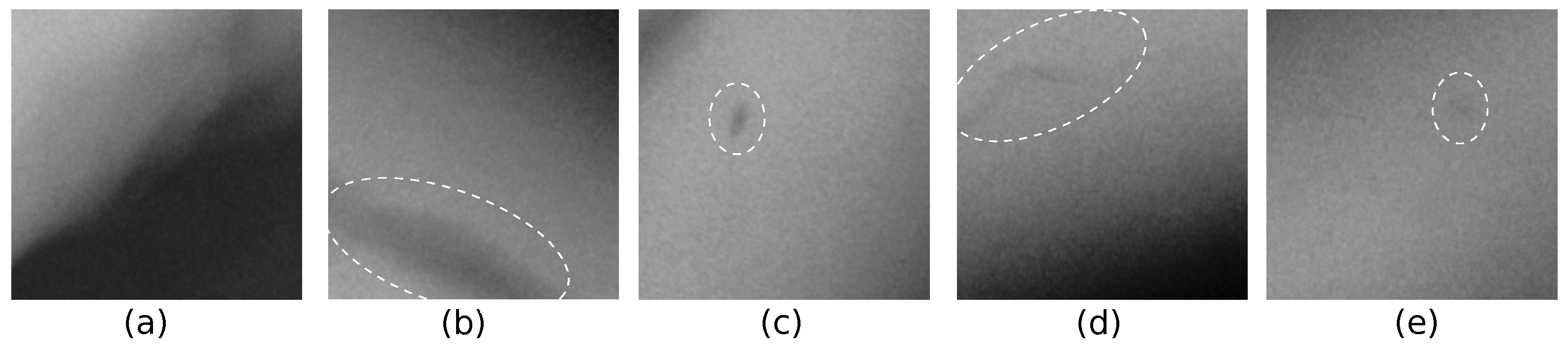
The weld dataset was divided into the following: training weld okay, training perturbed defects, test weld okay, and test defects. The test defect dataset was further divided by manual subjective characterization into three different contrast levels. See Figure 2 for the example patches. In addition, the test and training datasets were held separately on the weld image level. For the low contrast defects, it was not certain that a human operator would have a true positive rate close to 1 and a false positive rate close to 0. Moreover, it should be noted that the dataset is rather small for the application of deep learning; however, it is public and well-documented, making it a good candidate for this study.
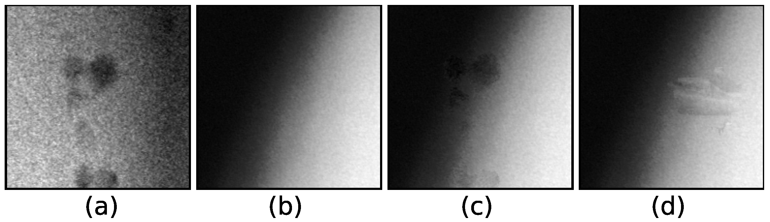
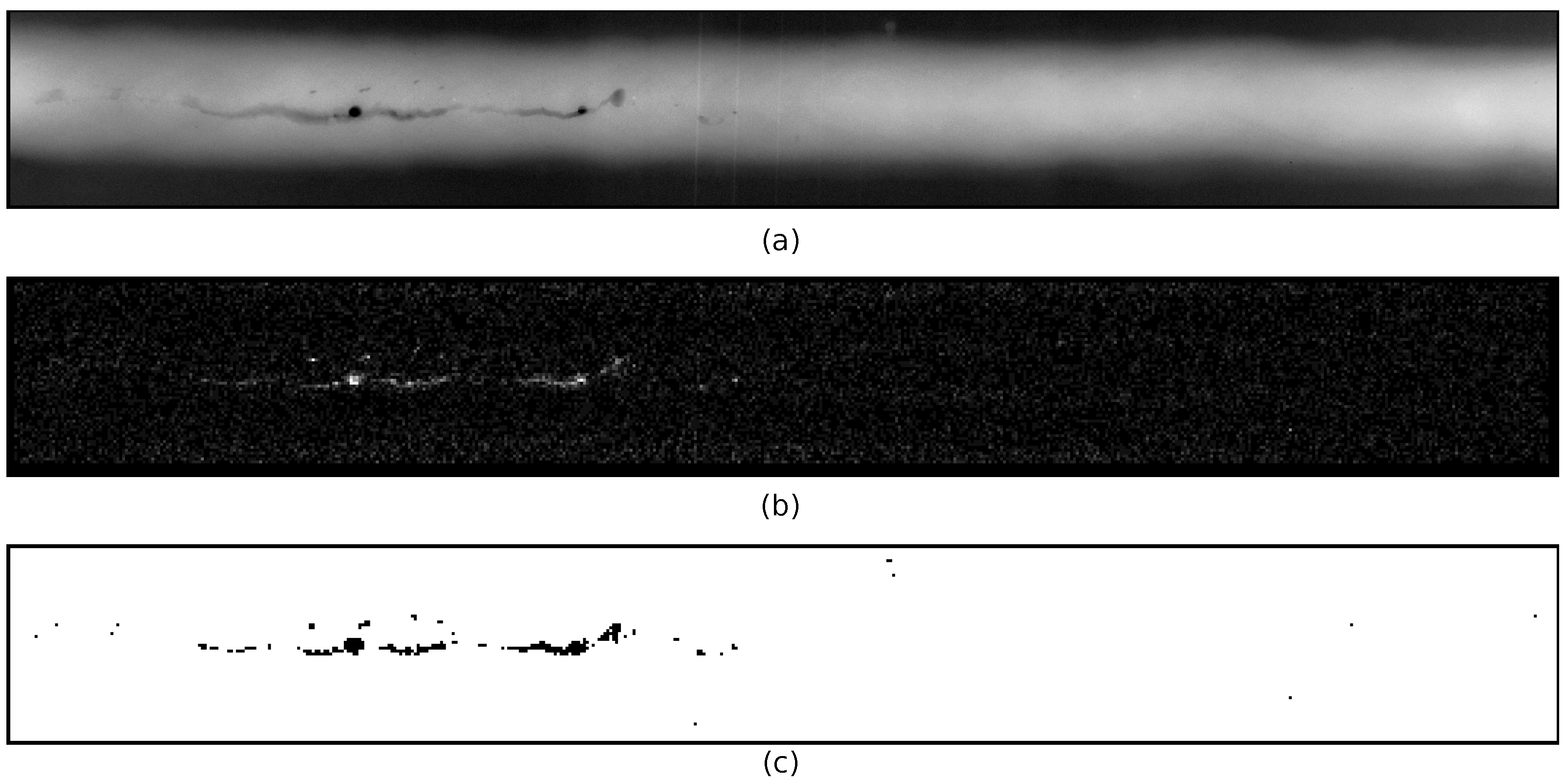
As described in the method section, patches with defect/anomaly indications were utilized during the AE model training to introduce perturbed weld okay patches. These perturbed defect patches were created in two steps. First, the pixel-level ground truth was utilized to separate the pixels marked as part of defects belonging to separate defect regions (segmentation), using a crude two-connectivity-based algorithm. For each region, the average intensity, over a border around it, was subtracted. Second, during training, random combinations of such patches and the weld okay dataset were added according to Equation (2). Some examples of the resulting perturbed patches are shown in Figure 3. The approach to add indications such as this into X-ray images is similar to the one utilized in [21].
For each of the above-mentioned datasets, patches of size were selected from the large input images by random translation and rotation (0–360) operations. Standard deep learning data augmentation was also conducted by duplicating the patches into samples at additional , , and angles as well as flipping up/down and left/right. The final dataset sizes, including augmentations, were the following: training weld okay, 164,724; training perturbed defects, 70,230; test weld okay, 3480; test defect, high (3396), mid- (2898), and low contrast (1830). Some parts of the patches were resampled and, thus, are not independent; however, there was no overlap between the test and train sets.
In addition, synthetic datasets were derived—one for extending the perturbed dataset during the AE model training and one for the training of the supervised–trained classifier as well as testing both of the models. These synthetic datasets were not presented in [37].
Ideally, the perturbed dataset should include all possible intensity variations other than the ones present in the accepted (okay weld) dataset. The hypothesis is that this will delimit the reconstruction capabilities of the AE model very close to only the accepted dataset. The synthetic perturbations do not have to be too similar to real weld defects, as they are ideally covered by real experimental data; moreover, unrealistic perturbations far from the training distribution are acceptable. We derived such a large perturbation dataset by random sampling regions from another unrelated dataset with visual images. The visual images utilized came from a highly unrelated publicly available dataset with natural images (6899 images with sizes at the order of ) of planes, motorbikes, flowers, and similar [58].
The derivation details of the synthetic perturbation dataset will be given since the idea behind the dataset is rather unconventional within the non-destructive evaluation application field. The perturbations are assumed to be irregularly shaped regions, with the size of each region smaller than the whole image patch. The intensity variation within each region was taken from the above-mentioned visual natural images by sampling such irregularly shaped regions from the natural image dataset. In detail, the shape distribution of the regions was derived by the following sampling rules: A random number of regions was sampled from the uniform random distribution , each with a randomly sized number of pixels by growing regions from a random seed position in the natural images. Iteratively, each region was grown by taking a step of , , or in either of the two dimensions. The shapes of the regions were partly controlled by an elongation parameter randomly sampled over , where e increases the probability of sampling 0 pixel steps in one of the dimensions, with probability given as . The regions were then masked and scaled in intensity (gray value) to 0.05–0.2, with the scale parameter uniform randomly sampled for each region. Finally, the regions were smoothed with Gaussian or Lorentzian point spread functions of random smoothness, the Lorentzian scale parameter (half width at half maximum) , and the Gaussian standard deviation . The lower limits of the smoothness parameters were approximated to represent the point spread function of the X-ray imaging setup utilized for deriving the real experimental X-ray images in the GD X-ray welds. Those perturbations, i.e., synthetic natural image indications (SNI), were then added to the accepted weld patches with the same procedures as for the real anomalies. An example can be seen in patch (d) in Figure 3. The SNI dataset was sampled to a size of 112,000 samples.
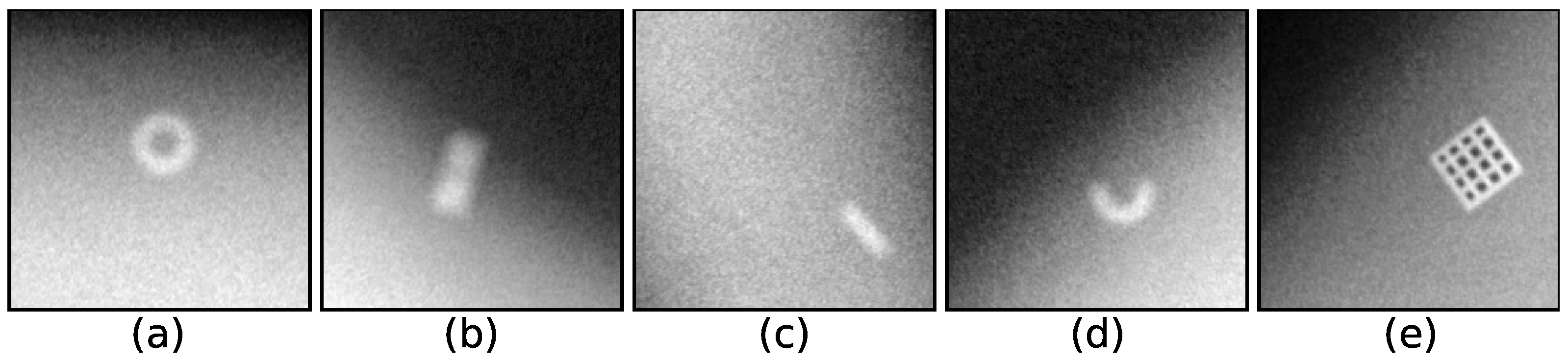
The synthetic datasets for extending the training dataset for the supervised–trained classifier and testing of both models were derived to have less variation than in the SNI case. The purpose of the test data was to set up OOD data examples, with some variations. The purpose of the training data, for the supervised–trained classifier, was to give a systematic example of the potential dangers with supervised–trained classifiers and the OOD test data. Six different types of synthetic defects and anomalies were derived (see Figure 4 for a few examples) with names indicating their characteristics, i.e., a circular hollow inclusion with an outer diameter of 36 px, an inner diameter of , and an amplitude of ; dogbone inclusion with a size of about and an amplitude of ; elongated inclusion with a size of about and an amplitude of ; partial circle inclusion (SPC) with an outer diameter of , inner diameter of , an amplitude of , and angle spread between 10 and 180; circular indication (SC) with a diameter randomly sampled and an amplitude of ; synthetic raster with a size of , and an amplitude of , representing a highly exotic unexpected OOD data example, e.g., a machine element or similar. All samples were randomly rotated and smoothed with a Gaussian point spread function prior to random placement into weld okay patches.
The sample sizes of the synthetic datasets used for testing were 200 samples each (circular hollow inclusion, dogbone inclusion, elongated inclusion, partial circle inclusion, raster), and those for training 5000 samples (circular indication, partial circle inclusion).
An overview of the datasets used in the study is given in Table 1. During the training, a random sample of perturbations is combined with a random sample of the augmented train weld okay; this can also be seen as an augmentation operation, leading to a larger effective size of the training dataset, i.e., at each training epoch a new combination of weld okay and perturbation dataset combination is sampled.
4. Results
Both of the two models have been trained several times on different training datasets, and then evaluated on both real and synthetic test datasets. For each training setup, training dataset combination, three independent models were trained and evaluated. The main performance evaluator scalars will be the true positive rate (TPR), average and the spread over the three models, at a fixed false positive rate (FPR). The results for the supervised–trained binary classifier will be reported first and then followed by the unsupervised–trained AE model.
The results for the supervised–trained patch-level binary classifier can be seen in Table 2. With just the weld okay and defects (D) as the training data, it is evident that for the synthetic indications (representing OOD data, see Figure 4) the TPR is low and, especially for the synthetic inclusions, with a rather large spread. By adding synthetic circular shaped indications (SC) to the training data, which is similar to the synthetic circular hollow inclusion as well as parts of the synthetic raster anomaly, those two test datasets are then better detected. Adding the synthetic partial circular inclusions (SPC) to the training data, further improves the detection of the synthetic anomalies; however, the elongated inclusion dataset, is still badly represented in the training data. Finally, by adding the synthetic natural image indications to the training data, all anomalies obtain high TPRs. The spread in the TPR results on the synthetic indications is overall lower for the D + SNI training case, however, still considerable for the elongated and partial circle anomalies.
Two use cases for the OOD detector, which are based on the unsupervised–trained AE model combined with the residual analysis, have been explored; one where the AE model is set up to model only accepted okay welds and one where it is set up to model both accepted and the known defects and anomalies.
The results for the first use case will be reported first, see Table 3. It can clearly be seen that training without a perturbation dataset considerably degrades the performance, indicating that even though the model is set up as a compressed representation learner it is capable of reconstructing also both real and synthetic defects at high precision. Adding the real defects (denoted by D in the table) to the perturbation dataset clearly remedies part of this, and the TPR is close to for the high contrast defect test dataset. Adding the synthetic natural image indications (SNI) to the perturbation dataset further drastically improves the results. In both cases where a perturbation dataset is present the AE model gives very high TPRs, with low spread, for the synthetic anomalies.
Representative examples of the reconstructions and residual images of the AE model for the different test datasets of real defects and synthetic anomalies can be seen in Figure 5, Figure 6, Figure 7 and Figure 8. The kernel residual image analysis results, both average and standard deviation, at FPR is also indicated. All of the AE models were trained with the SNI perturbation dataset.
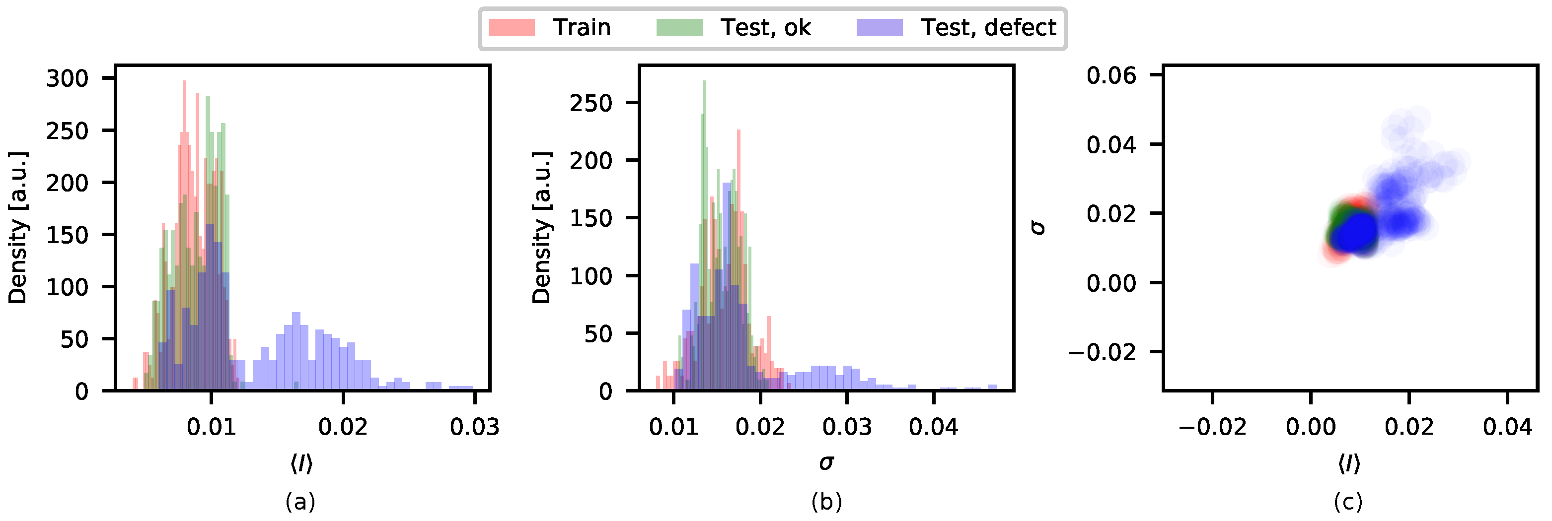
The residual image analysis results ( and kernels) can also be indicated as histograms to indicate the level of separation between the classes. The histograms for the high contrast real defects test dataset can be seen in Figure 9, AE model trained with SNI perturbations.
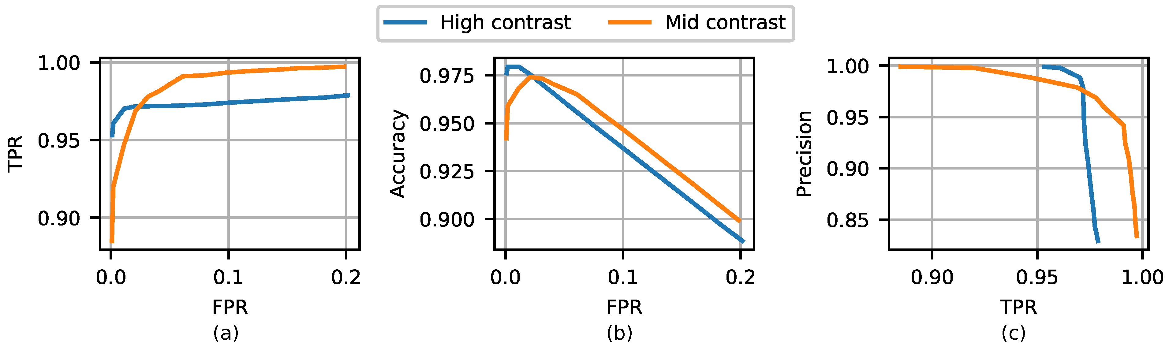
Curves over TPR and accuracy versus FPR, and precision versus TPR for the high and mid-contrast real defect test datasets are shown in Figure 10. All AE models trained with the SNI perturbation dataset.
The results of a sliding window analysis with the AE model trained with the SNI perturbation dataset are shown in Figure 11. Note that the model is not intended for an exact-as-possible segmentation, but rather it is intended to classify a patch-level, i.e., if it is to contain only an accepted weld or not; it offers some rough localization of where it did not.
A second OOD detector use case for the AE model, when it is trained to reconstruct both the accepted welds as well as the defects dataset, was also explored. In this setting, the AE model is trained to reconstruct also the defects as opposed to the first scenario or use case, where the AE maps perturbed inputs to the clean counterpart. The typical use case could be to utilize it as a pre-filtering OOD detection step before conducting, e.g., a conventional two-class pixel-wise segmentation with, e.g., a UNet. The residual image analysis results can be seen in Figure 12. No perturbation dataset was utilized, since the SNI dataset was suspected to overlap too much with the real defects. In this case, ideally, the kernel analysis scalars for the test defect dataset should overlap around a narrow peak close to zero. We do not reach as good results as for the case in Figure 9, with only weld okay as the training dataset, where instead the kernel scalars should be as separated as possible. However, even with this model, we can correctly detect (at FPR) the synthetic raster test anomaly as something unexpected (that a human should look into) as can be seen in Figure 13.
5. Discussion and Conclusions
In this study, we explored if an autoencoder-based convolutional deep neural network model could be utilized as an OOD detector algorithm within the application field of industrial X-ray image-based data interpretation. Such an OOD detector could then be interpreted as a quantitative estimation of the results’ confidence with respect to OOD data, or unexpected input data.
The model was trained unsupervised, to model (as in the reconstruction) the accepted training data, and forced to not reconstruct data dissimilar (called perturbation dataset) to the training data. The training was similar to the training of denoising autoencoders, with the perturbation dataset consisting of structural noise, similar to known and unknown/unexpected material imperfections or other anomalies.
The algorithm was explored on a real experimental dataset of X-ray images of metal fusion welds, with both defect-free accepted welds as well as welds with material defects. In addition, datasets with synthetic hypothetical material defects and anomalies were derived and used for training and testing.
On the real test data we achieved, at an image patch level, true positive rates were around and false positive rates were around . With only the real defects in the perturbation training dataset, the synthetic examples of unexpected input data were detected at rates close to with a low spread in the results. The best results were achieved with the perturbation dataset consisting only of synthetic OOD data examples. Indicating that the model could even be trained without real defect indications, only requiring real data representing the accepted welds. However, this is not entirely true since knowledge of the characteristics of potential material defects and anomalies (human input) were implicitly utilized when deriving the synthetic data.
The potential dangers of using supervised learners (e.g., UNet-like segmentation models) for interpreting industrial X-ray inspection images within quality critical applications was also exemplified. For this, a convolutional deep neural network model was derived and trained–supervised to classify patches as representing an okay weld or not. The network was trained on different datasets, with different similarities to the synthetic test data, to indicate the behavior of the in-distribution versus out-of-distribution test data. It was shown that the supervised–trained model (as expected) did show low average true positive rates with a large spread between the uniquely trained models for the synthetic test data not similar to the training data distribution.
Since (by nature) the unsupervised model is set up as a one-class classifier and the supervised as a binary classifier, one should be careful not to draw too many conclusions on the differences between the results for the two different models. However, the results of the in-distribution test data can be compared, and our results indicate that the model trained unsupervised was better or equal in performance compared to the model trained–supervised—this is an important comparison to make since most of the earlier studies on the same or similar datasets explored supervised–trained models.
In summary, we show that it is possible to train an autoencoder, unsupervised, with structural noise representing OOD data, to achieve the performances in the in-distribution test data that are higher than or similar to a model trained–supervised within the application field of industrial X-ray image interpretation. The model trained unsupervised was shown to excel over the model trained–supervised with respect to correctly detecting unexpected OOD test data. The proposed OOD detector can potentially facilitate the safe operation of computer-assisted data interpretation of industrial X-ray images within quality-critical industries. A trustworthy OOD detector would facilitate safe efficient cooperation between artificial intelligence and the human operator, where the AI could handle mundane data analysis of data similar to training and leave the OOD flagged data to the human operator.
Further research on this subject is required. For example, in order to evaluate and improve its suitability for industrial utilization, larger experimental datasets are required with more inherent variations. Moreover, larger datasets of unexpected OOD data are required in order to better understand how the performance of the unsupervised–trained model (e.g., sharpness in classification borders, true positive rates, and false positive rates) is affected by the perturbation dataset training approach.
Author Contributions
Conceptualization, E.L. and C.Z.; methodology, E.L. and C.Z.; software, E.L.; validation, E.L.; formal analysis, E.L.; investigation, E.L.; resources, E.L. and C.Z.; data curation, E.L.; writing—original draft preparation, E.L.; writing—review and editing, C.Z.; visualization, E.L. All authors have read and agreed to the published version of the manuscript.
Funding
This work was funded by the ÅForsk Foundation in Sweden, grant number 19-546.
Institutional Review Board Statement
Not applicable.
Informed Consent Statement
Not applicable.
Data Availability Statement
Not applicable.
Conflicts of Interest
The authors declare no conflict of interest.
References
- Wang, G.; Liao, W. Automatic identification of different types of welding defects in radiographic images. NDT&E Int. 2002, 35, 519–528. [Google Scholar]
- Dang, C.; Gao, J.; Wang, Z.; Xiao, Y.; Zhao, Y. A novel method for detecting weld defects accurately and reliably in radiographic images. Insight-Non-Destr. Test. Cond. Monit. 2016, 58, 28–34. [Google Scholar] [CrossRef]
- Silva, R.R.; Mery, D. State-ofthe-Art of Weld Seam Inspection by Radiographic Testing: Part I—Image Processing. Mater. Eval. 2007, 65, 643–647. [Google Scholar]
- Rathod, V.; Anand, R. A Comparative Study of Different Segmentation Techniques for Detection of Flaws in NDE Weld Images. J. Nondestruct. Eval. 2011, 31, 1–16. [Google Scholar] [CrossRef]
- Goodfellow, I.; Bengio, Y.; Courville, A. Deep Learning; The MIT Press: Cambridge, MA, USA, 2016. [Google Scholar]
- Kaftandjian, V.; Dupuis, O.; Babot, D.; Min Zhu, Y. Uncertainty modelling using Dempster–Shafer theory for improving detection of weld defects. Pattern Recognit. Lett. 2003, 24, 547–564. [Google Scholar] [CrossRef]
- Lashkia, V. Defect detection in X-ray images using fuzzy reasoning. Image Vis. Comput. 2001, 19, 261–269. [Google Scholar] [CrossRef]
- Wang, Y.; Sun, Y.; Lv, P.; Wang, H. Detection of line weld defects based on multiple thresholds and support vector machine. NDT&E Int. 2008, 41, 517–524. [Google Scholar]
- Vilar, R.; Zapata, J.; Ruiz, R. An automatic system of classification of weld defects in radiographic images. NDT&E Int. 2009, 42, 467–476. [Google Scholar]
- Kumar, J.; Anand, R.; Srivastava, S. Flaws Classification using ANN for Radiographic Weld Images. In Proceedings of the International Conference on Signal Processing and Integrated Networks, Noida, India, 20–21 February 2014; pp. 145–150. [Google Scholar]
- Dong, X.; Taylor, C.J.; Cootes, T.F. Automatic Inspection of Aerospace Welds Using X-ray Images. In Proceedings of the 2018 24th International Conference on Pattern Recognition (ICPR), Beijing, China, 20–24 August 2018; pp. 2002–2007. [Google Scholar]
- Nacereddine, N.; Goumeidane, A.B.; Ziou, D. Unsupervised weld defect classification in radiographic images using multivariate generalized Gaussian mixture model with exact computation of mean and shape parameters. Comput. Ind. 2019, 108, 132–149. [Google Scholar] [CrossRef]
- Mery, D.; Arteta, C. Automatic Defect Recognition in X-ray Testing using Computer Vision. In Proceedings of the 2017 IEEE Winter Conference on Applications of Computer Vision (WACV), Santa Rosa, CA, USA, 24–31 March 2017; pp. 1026–1035. [Google Scholar]
- Mu, Y.; Yan, S.; Liu, Y.; Huang, T.; Zhou, B. Discriminative local binary patterns for human detection in personal album. In Proceedings of the 2008 IEEE Conference on Computer Vision and Pattern Recognition, Anchorage, AK, USA, 23–28 June 2008; pp. 1–8. [Google Scholar]
- Hou, W.; Wei, Y.; Guo, J.; Jin, Y.; Zhu, C. Automatic Detection of Welding Defects using Deep Neural Network. J. Physics Conf. Ser. 2018, 933, 012006. [Google Scholar] [CrossRef]
- Hou, W.; Wei, Y.; Jin, Y.; Zhu, C. Deep features based on a DCNN model for classifying imbalanced weld flaw types. Measurement 2019, 131, 482–489. [Google Scholar] [CrossRef]
- Ronneberger, O.; Fischer, P.; Brox, T. U-Net: Convolutional Networks for Biomedical Image Segmentation. arXiv 2015, arXiv:cs.CV/1505.04597. Available online: https://arxiv.org/abs/1505.04597 (accessed on 14 November 2022).
- Tokime, R.B.; Maldague, X.; Perron, L. Automatic Defect Detection for X-ray inspection: Semantic segmentation with deep convolutional network. In Proceedings of the International Industrial Radiology and Computed Tomography DIR2019, Fürth, Germany, 2–4 July 2019. [Google Scholar]
- Tyystjärvi, T.; Virkkunen, I.; Fridolf, P.; Rosell, A.; Barsoum, Z. Automated defect detection in digital radiography of aerospace welds using deep learning. Weld. World 2022, 66, 643–671. [Google Scholar] [CrossRef]
- Yang, L.; Jiang, H. Weld defect classification in radiographic images using unified deep neural network with multi-level features. J. Intell. Manuf. 2021, 32, 459–469. [Google Scholar] [CrossRef]
- Mery, D. Aluminum Casting Inspection Using Deep Learning: A Method Based on Convolutional Neural Networks. J. Nondestruct. Eval. 2020, 39, 12. [Google Scholar] [CrossRef]
- Fuchs, P.; Kröger, T.; Dierig, T.; Garbe, C. Generating Meaningful Synthetic Ground Truth for Pore Detection in Cast aluminum Parts. In Proceedings of the 9th Conference on Industrial Computed Tomography, Padova, Italy, 13–15 February 2019. [Google Scholar]
- Cogranne, R.; Retraint, F. Statistical detection of defects in radiographic images using an adaptive parametric model. Signal Process. 2014, 96, 173–189. [Google Scholar] [CrossRef]
- Grandin, R.; Gray, J. Implementation of automated 3D defect detection for low signa-to noise features in NDE data. Aip Conf. Proc. 2014, 1581, 1840–1847. [Google Scholar] [CrossRef]
- Kazantsev, I.; Lemahieu, I.; Salov, G.; Denys, R. Statistical detection of defects in radiographic images in nondestructive testing. Signal Process. 2002, 82, 791–801. [Google Scholar] [CrossRef]
- Tošić, I.; Frossard, P. Dictionary Learning. IEEE Signal Process. Mag. 2011, 28, 27–38. [Google Scholar] [CrossRef]
- Chen, B.; Fang, Z.; Xia, Y.; Zhang, L.; Huang, Y.; Wang, L. Accurate defect detection via sparsity reconstruction for weld radiographs. NDT&E Int. 2018, 94, 62–69. [Google Scholar]
- Presenti, A.; Liang, Z.; Pereira, L.F.A.; Sijbers, J.; Beenhouwer, J.D. Automatic anomaly detection from X-ray images based on autoencoder. Nondestruct. Test. Eval. 2022, 37, 552–565. [Google Scholar] [CrossRef]
- Tang, W.; Vian, C.M.; Tang, Z.; Yang, B. Anomaly detection of core failures in die-casting X-ray inspection images using a convolutional autoencoder. Mach. Vis. Appl. 2021, 32, 102. [Google Scholar] [CrossRef]
- Meyendorf, N.G.; Bond, L.J.; Curtis-Beard, J.; Heilmann, S.; Pal, S.; Schallert, R.; Scholz, H.; Wunderlich, C. NDE 4.0—NDE for the 21st Century—The Internet of Things and Cyber Physical Systems will Revolutionize NDE. In Proceedings of the Proceedings of the 15th Asia Pacific Conference for Non-Destructive Testing (APCNDT 2017), Singapore, 13–17 November 2017. [Google Scholar]
- Rummel, W.D. Nondestructive inspection reliability history, status and future path. In Proceedings of the 18th World Conference on Nondestructive Testing, Durban, South Africa, 16–20 April 2010. [Google Scholar]
- Lindgren, E.; Forsyth, D.; Aldrin, J.; Spencer, F. ASM Handbook, Volume 17, Nondestructive Evaluation of Materials; ASM International: Almere, The Netherlands, 2018. [Google Scholar]
- Ewert, U.; Zscherpel, U.; Jechow, M. Essential Parameters and Conditions for Optimum Image Quality in Digital Radiology. In Proceedings of the 18th World Conference on Nondestructive Testing, Durban, South Africa, 16–20 April 2012. [Google Scholar]
- Kanzler, D.; Ewert, U.; Müller, C.; Pitkänen, J. Observer POD for radiographic testing. AIP Conf. Proc. 2015, 1650, 562. [Google Scholar]
- Bertović, M. Human Factors in Non-Destructive Testing (NDT): Risks and Challenges of Mechanised NDT. PhD Thesis, Technische Universitaet Berlin, Berlin, Germany, 1 September 2015. [Google Scholar]
- Aldrin, J.C.; Lindgren, E.; Forsyth, D. Intelligence augmentation in nondestructive evaluation. Aip Conf. Proc. 2019, 2102, 020028. [Google Scholar]
- Lindgren, E.; Zach, C. Autoencoder-Based Anomaly Detection in Industrial X-ray Images. In Proceedings of the 2021 48th Annual Review of Progress in Quantitative Nondestructive Evaluation, Virtual, 28–30 July 2021. [Google Scholar] [CrossRef]
- Richter, C.; Roy, N. Safe Visual Navigation via Deep Learning and Novelty Detection. In Proceedings of the Robotics Science and Systems, Cambridge, MA, USA, 12–16 July 2017. [Google Scholar]
- Gal, Y.; Ghahramani, Z. Dropout as a Bayesian Approximation: Representing Model Uncertainty in Deep Learning. In Proceedings of the 33rd International Conference on Machine Learning, New York, NY, USA, 19–24 June 2016; Volume 48, pp. 1050–1059. [Google Scholar]
- Lakshminarayanan, B.; Pritzel, A.; Blundell, C. Simple and Scalable Predictive Uncertainty Estimation Using Deep Ensembles. In Proceedings of the 31st International Conference on Neural Information Processing Systems, Long Beach, CA, USA, 4–9 December 2017; Curran Associates Inc.: Red Hook, NY, USA, 2017; pp. 6405–6416. [Google Scholar]
- Seeböck, P.; Waldstein, S.; Klimscha, S.; Gerendas, B.S.; Donner, R.; Schlegl, T.; Schmidt-Erfurth, U.; Langs, G. Identifying and Categorizing Anomalies in Retinal Imaging Data. arXiv 2016, arXiv:cs.LG/1612.00686. Available online: https://arxiv.org/abs/1612.00686 (accessed on 14 November 2022).
- Schölkopf, B.; Platt, J.C.; Shawe-Taylor, J.C.; Smola, A.J.; Williamson, R.C. Estimating the Support of a High-Dimensional Distribution. Neural Comput. 2001, 13, 1443–1471. [Google Scholar] [CrossRef]
- Schlegl, T.; Seeböck, P.; Waldstein, S.M.; Schmidt-Erfurth, U.; Langs, G. Unsupervised Anomaly Detection with Generative Adversarial Networks to Guide Marker Discovery. arXiv 2017, arXiv:cs.CV/1703.05921. Available online: https://arxiv.org/abs/1703.05921 (accessed on 14 November 2022).
- Goodfellow, I.J.; Pouget-Abadie, J.; Mirza, M.; Xu, B.; Warde-Farley, D.; Ozair, S.; Courville, A.; Bengio, Y. Generative Adversarial Networks. arXiv 2014, arXiv:stat.ML/1406.2661. Available online: https://arxiv.org/abs/1406.2661 (accessed on 14 November 2022). [CrossRef]
- Schlegl, T.; Seeböck, P.; Waldstein, S.M.; Langs, G.; Schmidt-Erfurth, U. f-AnoGAN: Fast unsupervised anomaly detection with generative adversarial networks. Med. Image Anal. 2019, 54, 30–44. [Google Scholar] [CrossRef]
- Tang, Y.; Tang, Y.; Han, M.; Xiao, J.; Summers, R.M. Abnormal Chest X-ray Identification With Generative Adversarial One-Class Classifier. arXiv 2019, arXiv:cs.CV/1903.02040. Available online: https://arxiv.org/abs/1903.02040 (accessed on 14 November 2022).
- Akcay, S.; Atapour-Abarghouei, A.; Breckon, T.P. GANomaly: Semi-Supervised Anomaly Detection via Adversarial Training. arXiv 2018, arXiv:cs.CV/1805.06725. Available online: https://arxiv.org/abs/1805.06725 (accessed on 14 November 2022).
- Lindgren, E.; Zach, C. Analysis of industrial x-ray computed tomography data with deep neural networks. In Proceedings of the Developments in X-ray Tomography XIII. International Society for Optics and Photonics, San Diego, CA, USA, 1–5 August 2021; SPIE: Bellingham, WA, USA, 2021; Volume 11840, p. 118400B. [Google Scholar] [CrossRef]
- Springenberg, J.T.; Dosovitskiy, A.; Brox, T.; Riedmiller, M. Striving for Simplicity: The All Convolutional Net. arXiv 2015, arXiv:cs.LG/1412.6806. [Google Scholar]
- Hou, X.; Shen, L.; Sun, K.; Qiu, G. Deep feature consistent variational autoencoder. In Proceedings of the 2017 IEEE Winter Conference on Applications of Computer Vision (WACV), Santa Rosa, CA, USA, 24–31 March 2017; pp. 1133–1141. [Google Scholar]
- Vincent, P. A connection between score matching and denoising autoencoders. Neural Comput. 2011, 23, 1661–1674. [Google Scholar] [CrossRef] [PubMed] [Green Version]
- Hyvärinen, A.; Dayan, P. Estimation of non-normalized statistical models by score matching. J. Mach. Learn. Res. 2005, 6, 95–709. [Google Scholar]
- Abadi, M.; Agarwal, A.; Barham, P.; Brevdo, E.; Chen, Z.; Citro, C.; Corrado, G.S.; Davis, A.; Dean, J.; Devin, M.; et al. TensorFlow: Large-Scale Machine Learning on Heterogeneous Systems. 2015. Available online: tensorflow.org (accessed on 14 November 2022).
- Kingma, D.P.; Ba, J. Adam: A Method for Stochastic Optimization. arXiv 2017, arXiv:cs.LG/1412.6980. [Google Scholar]
- Eckel, S.; Huthwaite, P.; Zscherpel, U.; Schumm, A.; Paul, N. Realistic Film Noise Generation Based on Experimental Noise Spectra. Trans. Imge Proc. 2020, 29, 2987–2998. [Google Scholar] [CrossRef]
- Lindgren, E.; Wirdelius, H. X-ray modeling of realistic synthetic radiographs of thin titanium welds. Ndt&E Int. 2012, 51, 111–119. [Google Scholar]
- Mery, D.; Riffo, V.; Zscherpel, U.; Mondragón, G.; Lillo, I.; Zuccar, I.; Lobel, H.; Carrasco, M. GDXray: The Database of X-ray Images for Nondestructive Testing. J. Nondestruct. Eval. 2015, 34, 42. [Google Scholar] [CrossRef]
- Roy, P.; Ghosh, S.; Bhattacharya, S.; Pal, U. Effects of Degradations on Deep Neural Network Architectures. arXiv 2018, arXiv:1807.10108. Available online: https://arxiv.org/abs/1807.10108 (accessed on 14 November 2022).
Figure 1.
Overview of the AE model with encoder () and decoder () blocks. Adapted from [37] with permission from ASME.
Figure 1.
Overview of the AE model with encoder () and decoder () blocks. Adapted from [37] with permission from ASME.

Figure 2.
Examples of patches in the training and test datasets: (a) is weld okay, accepted weld, (b,c) are high contrast defects, (d) is a mid-contrast defect, and (e) is a low contrast defect. Adapted from [37] with permission from ASME.
Figure 2.
Examples of patches in the training and test datasets: (a) is weld okay, accepted weld, (b,c) are high contrast defects, (d) is a mid-contrast defect, and (e) is a low contrast defect. Adapted from [37] with permission from ASME.

Figure 3.
Examples of perturbed defect patches in the training dataset; (a) real defect, (b) okay weld, (c) okay plus real defect patch, and (d) okay weld plus a synthetic natural image-based defect patch; (a–c) are adapted from [37] with permission from ASME.
Figure 3.
Examples of perturbed defect patches in the training dataset; (a) real defect, (b) okay weld, (c) okay plus real defect patch, and (d) okay weld plus a synthetic natural image-based defect patch; (a–c) are adapted from [37] with permission from ASME.

Figure 4.
Examples of synthetic defect and anomaly indications inserted into weld okay patches: (a) circular hollow inclusion, (b) dogbone inclusion, (c) elongated inclusion, (d) partial circle inclusion, and (e) raster.
Figure 4.
Examples of synthetic defect and anomaly indications inserted into weld okay patches: (a) circular hollow inclusion, (b) dogbone inclusion, (c) elongated inclusion, (d) partial circle inclusion, and (e) raster.

Figure 5.
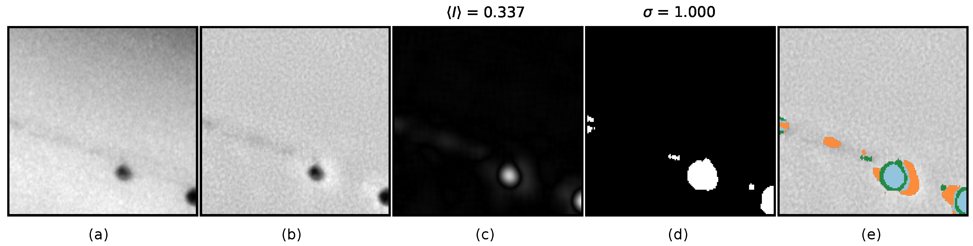
Results for the high contrast real defects test dataset; (a) is input, (b) is the residual image, residual analysis kernel results are for average kernel in (c) and standard deviation in (d). Above the patch is the maximum value indicated. Kernels above thresholds are indicated in (e) with blue ( and ), green (), and orange ().
Figure 5.
Results for the high contrast real defects test dataset; (a) is input, (b) is the residual image, residual analysis kernel results are for average kernel in (c) and standard deviation in (d). Above the patch is the maximum value indicated. Kernels above thresholds are indicated in (e) with blue ( and ), green (), and orange ().

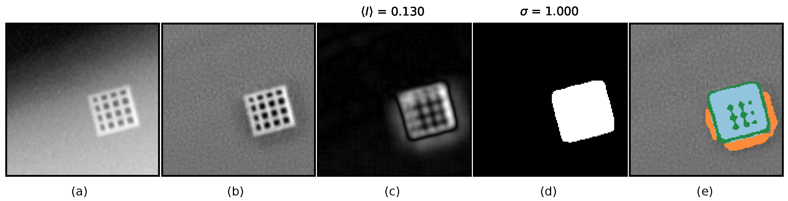
Figure 6.
Results for the mid-contrast real defects test dataset. (a) is input, (b) is the residual image, residual analysis kernel results are for average kernel in (c) and standard deviation in (d). Above the patch is the maximum value indicated. Kernels above thresholds are indicated in (e) with blue ( and ), green (), and orange ().

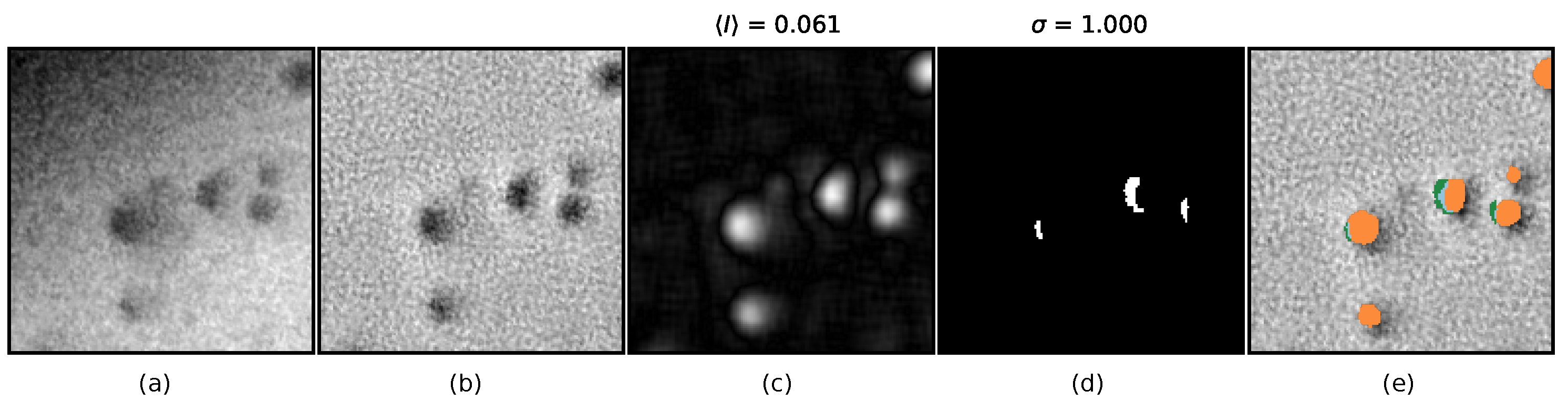
Figure 7.
Results for the synthetic partial circle inclusion test dataset. (a) is input, (b) is the residual image, residual analysis kernel results are for average kernel in (c) and standard deviation in (d). Above the patch is the maximum value indicated. Kernels above thresholds are indicated in (e) with blue ( and ), green (), and orange ().

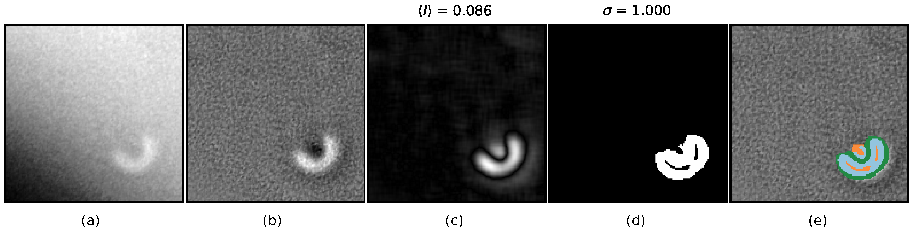
Figure 8.
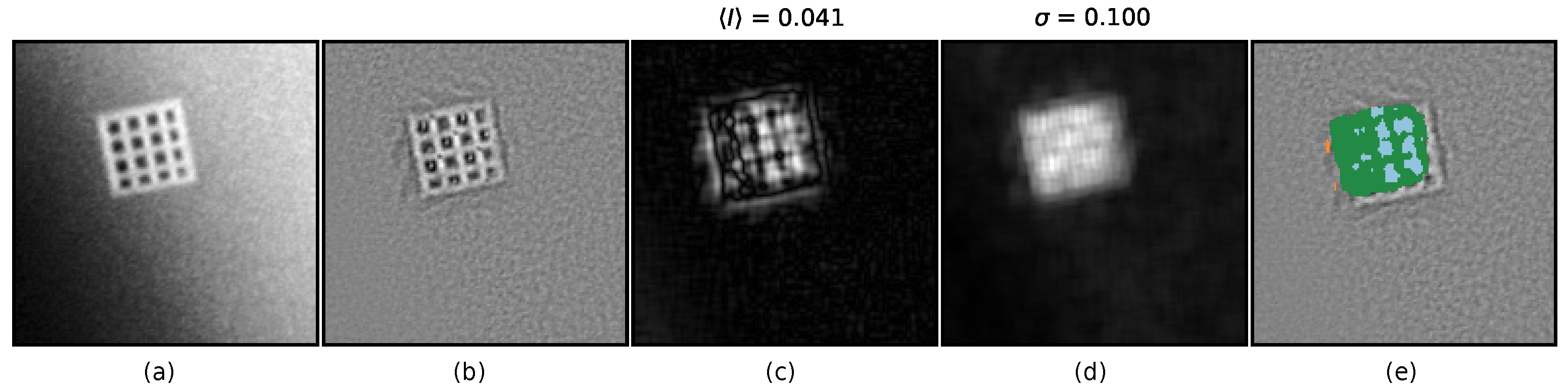
Results for the exotic synthetic raster anomaly. (a) is input, (b) is the residual image, residual analysis kernel results are for average kernel in (c) and standard deviation in (d). Above the patch is the maximum value indicated. Kernels above thresholds are indicated in (e) with blue ( and ), green (), and orange ().
Figure 8.
Results for the exotic synthetic raster anomaly. (a) is input, (b) is the residual image, residual analysis kernel results are for average kernel in (c) and standard deviation in (d). Above the patch is the maximum value indicated. Kernels above thresholds are indicated in (e) with blue ( and ), green (), and orange ().

Figure 9.
Residual image analysis results for the high contrast real defects test dataset. The distribution is given in (a), the distribution in (b), and in (c) versus is plotted. Observe that the histograms have different scales than the scatter plot.
Figure 9.
Residual image analysis results for the high contrast real defects test dataset. The distribution is given in (a), the distribution in (b), and in (c) versus is plotted. Observe that the histograms have different scales than the scatter plot.

Figure 10.
Receiver operating characteristics curve (a), accuracy versus false positives (b), and precision versus true positives (c) for the high and mid-contrast real defects test datasets. All values are in fractions.
Figure 10.
Receiver operating characteristics curve (a), accuracy versus false positives (b), and precision versus true positives (c) for the high and mid-contrast real defects test datasets. All values are in fractions.

Figure 11.
AE model sliding window results for the test dataset. Trained with the SNI perturbation dataset. (a) is the original input, (b) is the residuals, and (c) is the kernel analysis results thresholded with thresholds resulting in an FPR at on a patch level.
Figure 11.
AE model sliding window results for the test dataset. Trained with the SNI perturbation dataset. (a) is the original input, (b) is the residuals, and (c) is the kernel analysis results thresholded with thresholds resulting in an FPR at on a patch level.

Figure 12.
Kernel residual analysis results for the AE model trained on accepted welds as well as those with defects, but without any perturbation dataset. The distribution is given in (a), the distribution in (b), and in (c) versus is plotted.
Figure 12.
Kernel residual analysis results for the AE model trained on accepted welds as well as those with defects, but without any perturbation dataset. The distribution is given in (a), the distribution in (b), and in (c) versus is plotted.

Figure 13.
Results for the AE model trained on both accepted welds and those with defects, a synthetic raster anomaly test sample. (a) is input, (b) is the residual image, the residual analysis kernel results are for average kernel in (c) and standard deviation in (d). Above the patch is the maximum value indicated. Kernels above thresholds are indicated in (e) with blue ( and ), green (), and orange ().


Table 1.
Overview of the different datasets utilized. For the experimental data, the original sample count refers to the number of unique patches extracted with random translation and rotation from the original full-sized image input; for the synthetic data, the original sample count refers to the number of unique random realizations. See the text for details.
| Dataset | Original Sample Count | Augmented Sample Count |
|---|---|---|
| Train weld okay | 27,454 | 164,724 |
| Train defects | 11,705 | 70,230 |
| Train synthetic natural image indications | 112,000 | |
| Train synthetic, circular indication | 5000 | |
| Train synthetic, partial circle inclusion | 5000 | |
| Test weld okay | 3480 | |
| Test defect, high contrast | 3396 | |
| Test defect, mid-contrast | 2898 | |
| Test defect, low contrast | 1830 | |
| Test, synthetic, five different types | 200 |
Table 2.
Results for the supervised–trained patch-level binary classifier. The TPR is given as the average and the spread within parenthesis, at FPR. For the training data, D is for defects, SC is for synthetic circular indication, SPC is for synthetic partial circular inclusion, SNI is for synthetic natural image indications.
| TPR Average and Spread | ||||
|---|---|---|---|---|
| Training Data | D | D + SC | D + SC + SPC | D + SNI |
| Test Dataset | ||||
| Defects high contrast | ||||
| Defects mid-contrast | ||||
| Defects low contrast | ||||
| Synthetic circular hollow inclusion | ||||
| Synthetic dogbone inclusion | ||||
| Synthetic elongated inclusion | ||||
| Synthetic partial circle inclusion | ||||
| Synthetic raster | ||||
Table 3.
Results for the unsupervised–trained autoencoder model, OOD detector. The TPR is given as the average and the spread within parenthesis, at FPR. Results are shown for training with weld okay and different perturbation datasets, where D denotes the real defect dataset and SNI is the synthetic natural image indications dataset.
| TPR Average and Spread | |||
|---|---|---|---|
| Perturbation Dataset | None | D | SNI |
| Test Dataset | |||
| Defects high contrast | |||
| Defects mid-contrast | |||
| Defects low contrast | |||
| Synthetic circular hollow inclusion | |||
| Synthetic dogbone inclusion | |||
| Synthetic elongated inclusion | |||
| Synthetic partial circle inclusion | |||
| Synthetic raster | |||
Publisher’s Note: MDPI stays neutral with regard to jurisdictional claims in published maps and institutional affiliations. |
© 2022 by the authors. Licensee MDPI, Basel, Switzerland. This article is an open access article distributed under the terms and conditions of the Creative Commons Attribution (CC BY) license (https://creativecommons.org/licenses/by/4.0/).
Share and Cite
MDPI and ACS Style
Lindgren, E.; Zach, C. Industrial X-ray Image Analysis with Deep Neural Networks Robust to Unexpected Input Data. Metals 2022, 12, 1963. https://0-doi-org.brum.beds.ac.uk/10.3390/met12111963
AMA Style
Lindgren E, Zach C. Industrial X-ray Image Analysis with Deep Neural Networks Robust to Unexpected Input Data. Metals. 2022; 12(11):1963. https://0-doi-org.brum.beds.ac.uk/10.3390/met12111963
Chicago/Turabian StyleLindgren, Erik, and Christopher Zach. 2022. "Industrial X-ray Image Analysis with Deep Neural Networks Robust to Unexpected Input Data" Metals 12, no. 11: 1963. https://0-doi-org.brum.beds.ac.uk/10.3390/met12111963
Note that from the first issue of 2016, this journal uses article numbers instead of page numbers. See further details here.