
The Use of Machine-Learning Techniques in Material Constitutive Modelling for Metal Forming Processes


1
Centre for Mechanical Technology and Automation (TEMA), Department of Mechanical Engineering, University of Aveiro, 3810-193 Aveiro, Portugal
2
Department of Electronics, Telecomunications and Electronics, Institute of Electronics and Informatics Engineering of Aveiro (IEETA), University of Aveiro, 3810-193 Aveiro, Portugal
*
Author to whom correspondence should be addressed.
Metals 2022, 12(3), 427; https://0-doi-org.brum.beds.ac.uk/10.3390/met12030427
Submission received: 30 December 2021
/
Revised: 15 February 2022
/
Accepted: 23 February 2022
/
Published: 28 February 2022
(This article belongs to the Special Issue Recent Advances and Applications of Machine Learning in Metal Forming Processes)
Abstract
:Accurate numerical simulations require constitutive models capable of providing precise material data. Several calibration methodologies have been developed to improve the accuracy of constitutive models. Nevertheless, a model’s performance is always constrained by its mathematical formulation. Machine learning (ML) techniques, such as artificial neural networks (ANNs), have the potential to overcome these limitations. Nevertheless, the use of ML for material constitutive modelling is very recent and not fully explored. Difficulties related to data requirements and training are still open problems. This work explores and discusses the use of ML techniques regarding the accuracy of material constitutive models in metal plasticity, particularly contributing (i) a parameter identification inverse methodology, (ii) a constitutive model corrector, (iii) a data-driven constitutive model using empirical known concepts and (iv) a general implicit constitutive model using a data-driven learning approach. These approaches are discussed, and examples are given in the framework of non-linear elastoplasticity. To conveniently train these ML approaches, a large amount of data concerning material behaviour must be used. Therefore, non-homogeneous strain field and complex strain path tests measured with digital image correlation (DIC) techniques must be used for that purpose.
1. Introduction
Considerable developments in the field of computational mechanics and the growth in computational power have made it possible for numerical simulation software to emerge and completely revolutionize the engineering industry. In fact, industry’s high-demand-fuelled and fast-paced development cycles have accelerated the adoption of computational analysis software [1,2]. With a wide array of software solutions in the market, capable of virtualizing entire design workflows, numerical simulation has become a vital component of the product development process. Indeed, this virtualization has allowed companies to massively reduce the number of time-consuming experiments between design iterations, thus reducing delays and costs and allowing companies to reach higher levels of competitiveness [3]. In this context, finite element analysis (FEA) has been widely used as a powerful numerical simulation tool in engineering analyses, such as structural analysis, heat transfer and fluid flow. In FEA, the material behavior is defined by specific constitutive models for which the ability to adequately describe a given material directly impacts the reliability of the numerical results. As such, material characterization has received increasing attention given the need for computational analysis software for precise material data [3].
Conventionally, constitutive laws are established according to first-principle assumptions in order to generalize experimental observations made on simple loading regimes. In recent years, the fast development of complex materials exhibiting non-linear behavior has pushed the formulation of advanced and more complex constitutive models to accurately describe phenomena such as hardening and anisotropy. The challenge lies in reducing the error between the numerical predictions and the experimental value. To improve this differential, the models are enhanced with additional empirical parameters, albeit with the cost of adding complexity to the empirical expressions and making them more difficult to calibrate [4,5]. Although the advances in imaging techniques, such as DIC, have allowed for much richer information to be extracted from experimental observations, conventional models are sometimes incompatible with the abundance of data [6,7]. However, independently of a model’s flexibility to adapt to the experimental results, it is always limited by its mathematical formulation, as it is written explicitly. Additionally, even if a model could be perfectly calibrated for a given set of experiments, there is no guarantee that it would provide a perfect result for a different set of experiments [8].
In recent years, the advent of Big Data combined with improved algorithms and the exponential increase in computing power led to an unprecedented growth in the field of artificial intelligence (AI) [9]. AI techniques, such as ML, allow computer systems to implicitly learn and recognize patterns purely based on data. For this reason, ML has become an important technology in various engineering fields [10]. Out of all ML algorithms, ANNs are extremely popular given their superior modelling performance in a wide range of applications, including as universal function approximators [10,11]. As such, neural networks have the potential to provide a radically different approach to material modelling, with the main advantage that it is not necessary to postulate a mathematical formulation or identify empirical parameters [12]. In general, data-driven approaches can better exploit the large volumes of data from modern experimental measurements, while avoiding the bias induced by constitutive models [6]. These ML techniques rely on different methods to determine the stress tensor corresponding to a given strain state (and other conditions such as temperature, strain rate, etc.). For instance, in [7,8], nearest neighbour interpolation is employed, while in [13,14,15,16], the authors employ a low-dimensional representation of the constitutive equation based uniquely on data. Bessa and co-workers [17] employ clustering techniques, while others employ spline approximations. ANNs were also used for modelling viscoplasticity behaviours [18,19]. Alternative solutions to pure data-driven models were given, namely hybrid models [15], that enhance/correct existing well-known models with information coming from data, thus performing a sort of data-driven correction. However, there is no consensus about the best data-driven strategy. Even regarding ML methods, different models were employed. In [18], a multi-layer feedforward neural network (FFNN) is presented. In turn, in [20], a nested adaptive neural network (NANN) is proposed as a variation of a standard FFNN. On [19,21], both authors use a FFNN with error backpropagation, but in [19], the algorithm is modified and based only on the error of the strain energy and the external work without the need for stress data. The major problem of data-driven and ML models is that their accuracy depends on the data used for training, including its quality and quantity. These models require massive amounts of necessarily dissimilar data [22]. However, most data obtained from mechanical tests, even heterogeneous tests, are similar in strain states [23]. Therefore, new mechanical tests are needed to extract the large quantity/quality of material behaviour data needed to accurately train these models.
The objective of this paper is to present, analyse and discuss the potential of ML models, particularly of ANNs, in material constitutive modelling for mechanical numerical simulations. The contribution of ANNs in material constitutive behaviour discussed in this paper includes the following approaches: (i) parameter identification inverse methodology, (ii) constitutive model corrector, (iii) data-driven constitutive model using empirical known concepts and (iv) general implicit constitutive model using data-driven learning approach. In this paper, special emphasis is given to implicit data-driven material modelling, and a dedicated state-of-the-art review is included. Nevertheless, examples of all previous approaches are given in the framework of non-linear elastoplasticity and full-field analysis.
The paper is structured as follows: in Section 2, the fundamentals of the conventional approach to material modelling are briefly explained and the mathematical formulations applied to elasticity and plasticity are introduced. In Section 3, the application potential of ML/ANNs to different sub-fields of material constitutive modelling is discussed, while also introducing the concept of implicit material modelling. In Section 4, a literature review on the latter topic is presented, as well as a discussion concerning its implementation into FEA codes; finally, in Section 5, concrete application examples of the different approaches discussed in Section 3 are presented.
2. Classical Material Modelling
2.1. Phenomenological Approach
Material modelling refers to the development of constitutive laws representing the material behavior at the continuum level. Conventionally, constitutive laws are developed based on simplified assumptions and empirical expressions. Such expressions rely on empirical parameters, computed or calibrated via experimental methods. The calibration process ensures the compatibility between the observed and numerically simulated mechanical responses [5,24]. As models become more advanced in their physical basis, empirical expressions get more complex, often requiring extensive experimental campaigns [2].
The highly complex nature of material behavior and the research of new materials in recent years has led to the development of a great number of constitutive models targeting different phenomena. In the framework of plasticity, one can highlight the classic models by Tresca, von Mises [25] or Hill [26]. Such models are formulated as flow rules based on the yield function of the material.
2.2. Elastoplasticity
A material under load suffers plastic deformation starting at the uniaxial yield stress . Beyond this point, hardening phenomena take place. Reversing the load at a given strain , plastic deformation ceases and stress starts to linearly decrease with strain, with a gradient equal to the Young’s modulus, E [27]. Once the stress reaches zero, the strain remaining in the material is the plastic strain , whereas the recovered strain is the elastic strain. The following relationships are easily derived [25]:
There are plenty of developed yield criteria, with the most commonly used in engineering practice being that of von Mises. The criterion relies on the knowledge of an equivalent stress , the von Mises stress, defined in tensor notation as [27]:
where is the deviatoric stress tensor. Similarly, an effective plastic strain rate can be established, such that:
The yield function, thus, assumes the following representation [27]:
written here as a function of the stress and accumulated plastic strain p, such that:
The performance of the material thus depends on the previous states of stress and strain, that is, plasticity is path-dependent [18]. In this case, the plastic range can be characterized by two internal variables: the back stress tensor , representing kinematic hardening and the drag stress R representing isotropic hardening. The yield function is, therefore, modified as [27]:
where k is a material constant and J is a distance in the stress space. For large deformations, the elastoplaticity can be formulated based on the co-rotational configuration. An in-depth overview of this can be seen in [28].
3. Machine Learning Approaches for Constitutive Modelling in Metal Forming
Material constitutive models are mathematical formulations representing the main characteristics, behaviours and functions of the materials. Generally, continuum mechanical models, such as the ones presented in Section 2, are written in a differential form and require a calibration procedure. However, even with a very robust calibration, known in the field as parameter identification, the accuracy of the model is always constrained by its mathematical formulation. Additionally, the development of analytical constitutive models requires a large effort in both time and resources. Today’s state-of-the-art constitutive models required decades to develop and validate. However, there is still a margin for multiple improvement opportunities, particularly using ML techniques, such as the one presented in Appendix A. The most straightforward fields of application are the following:
3.1. Parameter Identification Inverse Modelling
One category of inverse problems in metal forming is called parameter identification. The aim is to estimate material parameters for constitutive models, i.e., estimate parameters to calibrate the models. The development of new materials and the effort to characterize the existent ones led to the formulation of new complex constitutive laws. Nevertheless, many of these new laws demand the identification of a large number of parameters adjusted to the material whose behaviour is to be simulated. In cases where the number of parameters is high, it might be necessary to solve the problem as an inverse non-linear optimization problem.
The parameters’ determination should always be performed confronting mathematical/numerical and experimental results. Therefore, the comparison between the mathematical model and the experimental results (observable data) is a function that must be evaluated and minimized. This is generally the objective function of these problems [29,30,31].
When using the finite element method (FEM) to reproduce the material behaviour, the most commonly used method is the finite element model updating (FEMU) technique, which consists of creating a FEM model of a mechanical test, collecting displacement or strain components at some points/nodes and calculating a cost function with the difference between numerical and experimental displacements at these nodes. Minimizing this cost function concerning the unknown constitutive parameters provides the solution to the problem. This method is very general and flexible and can be used with local, average or full-field measurements. Other methods have been also proposed, such as the constitutive equation gap method (CEGM), the equilibrium gap method (EGM), the reciprocity gap method (RGM) and the virtual fields method (VFM) [32]. A review of these methods can be found in [2].
Considering the direct problem, which is to obtain the strain, displacement and stresses given the input variables (such as boundary conditions, geometry, and material parameters), an inverse problem can be devised in a given way to obtain the material parameters and stresses, when the inputs are the geometry, boundary conditions, displacements, and strains. In this context, ML can be used to solve the inverse problem efficiently, modelling the inverse process using the direct problem results as training data. The solution for the direct problem can be easily obtained using FEA software. This approach is illustrated in Figure 1.
3.2. Constitutive Model Corrector
In the last decades, a large number of analytical constitutive models were developed. Although a large effort has been put in these successive developments, a model is always a simplification of reality and is always constrained by a mathematical formulation. Nevertheless, the effort and the knowledge gained in these last decades should not be neglected for the development of new constitutive models. Therefore, one approach to develop new constitutive models using ML techniques can take advantage of this knowledge, as a starting point, and can be used as what can be called a model corrector or model enhancement.
The approach of the model corrector starts after the calibration of the well-known analytical model. It consists of confronting the real observations, generally from experimental tests, with the numerical simulations. After the parameter identification process, the differences between the real and numerical values can be collected and evaluated in a way similar to a data decomposition process (see Figure 2). These differences do not come only from the errors of the measurement techniques but also from the limitations (non-mathematical flexibility) of the analytical model. Then, the ML model is used to model the differences as a different (refined) scale model.
For accurate simulations, both analytical and ML corrector models must be introduced in the FEA software, resulting in a hybrid constitutive model.
3.3. Data-Driven Constitutive Model Using Empirical Known Concepts
An upper level of the previous approaches is using ML exclusively to model the behaviour of the material. However, the architecture and the development of the ML model considers some physical and empirical knowledge gained in the last decades in the development of analytical models, which are numerically implemented a posteriori. An example of this influence is the selection of the input and output features of the ML model. Generally, these ML material models that use empirical knowledge are developed in a differential point of view, such as the known analytical models, and all output features are time-derivatives of the input features. Additionally, all features, including internal variables, have specific physical or empirical representations or concepts, such as hardening, grain size, recovery, etc.
These ML material models can easily fully replace the existent constitutive models implemented in FEA software because both share the same type of structure and input/output features (see Figure 3). Although the majority of the implementations are done explicitly, these models can theoretically be implemented in implicit FEA codes, such as ABAQUS [22]. To train these models, a non-straightforward analysis and decomposition of the experimental data is required for each specific feature of the model. This procedure takes into account the meaning of each feature (i.e., of each internal variable).
3.4. General Implicit Constitutive Model Using Data-Driven Learning Approach
The use of ML technology to fully model the behaviour of the material without any preconception, knowledge, analytical or mathematical formulation is the ultimate goal of this scientific thematic. Although not mature, this approach has a large potential because (i) the material behavior is caused by a multitude of phenomena too complex to be handled individually, as it is traditionally done in the development of analytical models; (ii) the amount of data now retrieved using full-field methods and heterogeneous tests is difficult to be analysed in the same way as the data previously acquired from classical homogeneous mechanical tests and (iii) no previous concepts or knowledge are required, and preconceptions can mean constraints for disruptive developments.
An illustration of the development of an ML constitutive model using full-field experimental data and its integration into FEA simulation software is depicted in Figure 3. The most difficult step in the development of this approach is training the model, which, in this case, does not use any physical knowledge as a training constraint. Additionally, output features of the model, such as components of the stress tensor, cannot be measured in real experimental mechanical tests.
4. Review on Implicit Data-Driven Material Modelling
The concept of implicit material modelling relies on the material behavior being captured within the connections of an ANN trained using experimental or even synthetic data. That is, the relationships between stress and strain are learned purely based on data without resorting to a mathematical model or any kind of assumptions. The neural network should not only be able to reproduce the data it was trained on, but also possess the ability to approximate the results of other experiments. In this regard, while explicit material models may often not be able to reproduce new sets of experiments [8], ANNs are highly flexible and adaptable in the sense that these can be improved by being retrained with new data [33,34].
The possibility of extending neural network concepts to constitutive modelling was first explored by Ghaboussi, Garret and Wu [35]. The authors trained feedforward neural networks with backpropogation using experimental data and tested them against several well-known analytical models describing the behavior of concrete in plane stress subjected to two load settings: monotonic biaxial loading and uniaxial compressive cyclic loading. For the first setting, both stress and strain-controlled models were developed in order to tackle the path dependency of the material behaviour. The models were trained to predict strain and stress increments, respectively, using the current states of stress and strain as inputs, with the addition of a stress or strain increment. For the cyclic load setting, the model was trained to predict the strain increment based on the current state and the previous two states of stress and strain. The authors reported promising results for both load settings with the ANN-based models showing, in some cases, better performance than some of the analytical formulations. With their research, Ghaboussi and coworkers effectively proved the powerful interpolation and generalization capabilities of ANNs applied to constitutive modelling tasks, thus laying the foundations for the further development of implicit material models. Their methodology was later applied to the constitutive modelling of concrete (Wu and Ghaboussi [36]), sand (Ghaboussi et al. [37] and Ellis et al. [38]) and composites (Ghaboussi et al. [39]).
An early application of the implicit modelling approach in the framework of metal plasticity is due to Furukawa and Yagawa [18]. The authors introduced the first mathematical description of the concept relying on a state-space representation and proposed an implicit viscoplastic model using neural networks based on the well-known Chaboche’s model. The model was trained using synthetic data and was tested against experimental data. Due to the fact that the internal variables of the Chaboche’s model are not experimentally obtainable, a simple technique was proposed in order to derive the states of kinematic and isotropic stresses from the experimental curves. Overall, the authors reported that the implicit model correlated well with the results provided by the conventional formulations when applied to testing data within the training range, certifying the great interpolative capacity of the neural network. However, considerable errors were observed in stress and stain curves when using testing data far off the limits of the training set, indicating the limited generalization capacity of the model.
Following a purely data-driven approach, several authors successfully applied very similar methodologies to train ANN-based constitutive models using experimental data to predict the flow behavior of different metals under hot deformation (i.e., compression, torsion). Many industrial and engineering applications require the hot deformation of materials which are associated with numerous metallurgic phenomena, affecting the structure of the material at the micro-scale. As such, several factors affecting the flow stress generate highly complicated and non-linear relationships, limiting the application range and accuracy of the conventional constitutive models. Li et al. [40] studied the high temperature flow characteristics of Ti–15–3 alloy for the determination of hot-forging processing parameters and used an ANN model to predict the flow stress, finding that the ANN was able to correctly reproduce the behavior in sampled and non-sampled data. Lin et al. [12] used an ANN to predict the flow stress of 42CrMo steel under hot compressive deformation tests, reporting that the predictions were in good agreement with the experimental results. Mandal et al. [41] stated that the ANN-based model was an efficient tool to evaluate and predict the deformation behavior of stainless steel type AISI 304L. Sun et al. [42] developed a constitutive relationship model for Ti40 alloy and indicated the predicted flow stress by the ANN-based model correlated well with experimental results. Li et al. [43] reported that an ANN-based model showed better performance and proved to be more accurate and effective in predicting the hot deformation behavior of modified 2.25Cr–1Mo steel than the conventional constitutive equations.
4.1. Neural Network Architectures and Generalization Capacity
The implicit approach to material modelling based on ANNs presents obvious advantages; however, important choices regarding network architecture and the training process have to be taken into account in order to avoid limited predictive capabilities. For example, non-linear material behavior is highly path-dependent, making it difficult for ANNs to learn and generalize well the full spectrum of material behavior. The issue is accounted by Ghaboussi and coworkers [35] in their original work. Aiming to improve the generalization capacity of the ANN-based material models, Ghaboussi and Sidarta [20] later proposed a new neural network architecture: nested adaptive neural networks (NANNs). Their proposal is based on the fact that most data have an inherent structure which, in the case of material behavior, is a nested structure that can be observable in terms of:
- Dimensionality—where constitutive funtions are taken as members of function spaces, each of which is contained in a space of subsequently higher dimensions;
- Path-dependency—where a state of the material behavior represented with a given number of history points is a subset of another state represented with a larger number of history points.
In line with this notion, the underlying concept of NANNs is to train a base module to represent the material behavior in the lowest function space and, subsequently, augment it with additional modules representing higher function spaces (Figure 4). All the nodes in each layer of the new added module are connected to all the nodes in the next layer of the lower levels. Each module is a standard FFNN trained using adaptive evolution; that is, neurons are subsequently added to the hidden layers as network approaches its capacity. With new nodes, new connections are generated, and the objective is for the new links to capture the knowledge that the old ones were not able to capture. As such, training is carried out for the new connections while the old ones are frozen. With this new technique, Ghaboussi and Sidarta [20] reported a significant error reduction when using high-level NANNs.
In more recent works, regarding the scope of the path-dependency of material behavior, several authors (Abueidda et al. [44], Heider et al. [45], Ghavamian and Simone [46], Mozaffar et al. [47] and Gorji et al. [48]) demonstrated that RNNs can be particularly useful for modelling path-dependent plasticity, reporting superior performance compared to conventional ANNs. Contrarily to the latter, RNNs are designed to handle time sequences [47,49] and are equipped with history-dependent hidden states, enabling them to carry information from previous inputs onto future predictions. These internal variables have the potential to emulate the role of objects such as plastic strains and back stresses in physics-based plasticity. Nevertheless, standard RNNs suffer from vanishing/exploding gradients that hinder the error backpropagation process while dealing with long sequences. Long short-term memory (LSTM) and GRUs are more robust derivations of the standard RNNs (Figure 5) proposed to avoid those problems.
Apart from generalization issues, a much more fundamental problem is emphasized by several authors [20,35,50,51]: the “black-box” nature of ANNs does not guarantee the implicit material model to obey the conservation laws, symmetry and invariance requirements of conventional models. Nonetheless, if a neural network has been trained with a comprehensive dataset, it is reasonable to assume that it would be able to approximate the laws that the actual material obeys and use its generalization capability to appropriately predict stress-strain paths not included in the training data. However, building comprehensive datasets means acquiring large amounts of data. The cost of acquition is often prohibitive, and models end up being built in a small data regime.
To tackle these issues, Raissi et al. [51] proposed a new type of neural network: physics-informed neural networks (PINNs). The authors exploit the use of automatic differentiation to differentiate neural networks with respect to their input coordinates (i.e., space and time) and model parameters to obtain PINNs. The technique allows to constrain neural network models to respect symmetries, invariances, or conservation principles originating from the physical laws that govern the observed data. This type of information, encoded in such a way into the neural network, acts as a regularization agent that greatly reduces the space of admissible solutions. The methodology was proven by the authors as able to tackle a wide range or problems in computational science, allowing the use of relatively simple FFNN architecture trained with small amounts of data. The general methodology proposed by Raissi and coworkers [51] was applied to constitutive modeling in a recent work by Masi et al. [50] through the proposal of thermodynamics-based artificial neural networks (TANNs), a subtype of PINNs. In TANNs, basic laws of thermodynamics are encoded directly in the architecture of the neural network. In the framework of material modelling, these thermodynamic constraints concern the stresses and the internal state variables and their relationship with the free-energy and the dissipation rate. Masi and coworkers [50] report that TANN-based models were able to deliver thermodynamically consistent predictions both for seen and unseen data, achieving more accurate results than standard ANN material models. Moreover, the authors state that the inclusion of the laws of physics directly into the network architecture allows for the use of smaller training datasets given that the network already does not have to capture the underlying relationships from data.
Xu et al. [52], on the other hand, note that even though these physical constraints allow for improved accuracy in stress predictions, ANN-based constitutive models may still not yield a symmetric positive definite stiffness matrix. Therefore, nonphysical solutions and numerical instabilities arise when coupling ANN-based models with FEM solvers. The authors propose symmetric positive definite neural networks (SPD-NN) as a new architecture in order to deal with these issues. The neural network model is trained to predict the Cholesky factors of the tangent stiffness matrix, from which the stress is obtained. According to Xu et al. [52], the approach weakly imposes convexity on the strain energy function and satisfies the Hill’s criterion and time consistency for path-dependent materials. The authors compared the SPD-NN with standard architectures in a series of problems involving elasto-plastic, hyper-elastic and multi-scale composite materials. The results showed that, overall, the SPD-NN was able to provide superior results, proving the effectiveness of the approach for learning path-dependent, path-independent and multi-scale material behaviour.
4.2. Integration in Finite Element Analysis
An ANN-based constitutive model can be used in a way similar to conventional material models in FEA to solve boundary value problems. An important disadvantage regarding the numerical implementation of ANN-based material models in FEA was pointed out by Ghaboussi and Sidarta [20]. The issue is related to the fact that the ANN model already provides an updated state of stress, without the need for integration of the model’s equations over the strain increment. Therefore, it is not possible to obtain an explicit form of the material’s stiffness matrix. As a solution, the authors propose an explicit formulation of the material’s stiffness matrix for the ANN-based material model, allowing for an efficient convergence of the finite element Newton–Raphson iterations.
Successful embedding of ANNs as material descriptions in finite element (FE) codes were recorded by several authors. Usually, the ANN architecture is implemented in the software’s subroutines as a set of matrices containing the optimized weights obtained during training. Substantial gains in computational efficiency using ANNs have been reported due to the practically instantaneous mapping offered by the ANNs. Lefik and Schrefler [21] trained a simple ANN as an incremental non-linear constitutive model for a FE code and demonstrated that a well-trained, albeit simple, network model was able to reproduce the behavior from simulated material hyteresis loops.
Kessler et al. [53] developed an ANN-based constitutive model for aluminum 6061 based on experimental data for different temperatures, strains and strain rates. The authors implemented the model in Abaqus VUMAT and reported the ANN’s superior ability to mirror the experimental results.
Jang et al. [10] proposed a constitutive model to predict elastoplastic behavior for J2-plasticity, where an ANN was implemented in Abaqus User MATerial (UMAT) to replace the conventional nonlinear stress-integration scheme under isotropic hardening. The ANN was used only for nonlinear plastic loading, while keeping linear elastic loading and unloading relegated to the physics-based model. The authors reported that the ANN-based model provided results in good agreement with those from the conventional model for single-element tensile test and circular cup drawing simulations.
Zhang and Mohr [54] rewrote a standard algorithm for von Mises plasticity such that the stress update was governed by a single non-linear function predicting the apparent modulus (i.e., the Young’s modulus in case of elastic loading/unloading, and the elastoplastic tangent matrix in case of plastic loading). This function was then replaced by an FFNN and implemented as a user material subroutine in Abaqus/explicit. The authors demonstrated that a neural network with 5 hidden layers and 15 neurons per layer was able to “learn” the yield condition, flow rule and hardening law from data, providing highly accurate responses to the predictions of a J2 plasticity model, including the large deformation response for arbitrary multi-axial loading paths and reverse loading.
4.3. Indirect/Inverse Training
The vast majority of the approaches documented in the literature for implicit constitutive modelling consists of feeding the ANN with paired data (usually, stress and strain) during the training process in order to assimilate the material behavior [55]. The process requires copious amounts of data, and obtaining comprehensive stress-strain relationships while relying on the standard simple mechanical tests poses a great challenge, especially when dealing with anisotropic materials. Moreover, in a complex experiment, certain variables such as stresses cannot be directly measured [56]. Therefore, the training process must be carried out in such a way that allows the ANN-based model to indirectly predict the stress using measurable data, e.g., displacements and global force, obtained from full-field measurements [56]. One of the first approaches to bypass these limitations was proposed by Ghaboussi et al. [39], consisting of an auto-progressive method to train an ANN to learn the behavior of concrete from experimental load–deflection curves. However, the method is inefficient due to the fact that FEM simulations are needed in order to compute the stress and strain.
The generalized SPD-NN architecture proposed by Xu et al. [52] was able to deal with both direct and indirect training procedures. For the latter, the authors used displacement and force data to indirectly train the SPD-NN-based model and predict the stress in an incremental form by coupling the ANN with a non-linear equation solver. Despite providing superior results compared to standard architectures, the authors point out the requirement of full-field data as the main limitation, especially for three-dimensional solid bodies.
Both Huang et al. [56] and Xu et al. [57] proposed a method to use an ANN to replace the constitutive model in a FEM solver in order to impose the physical constraints during training, enabling the ANN to learn material behaviour based on the experimental measurement. Nonetheless, the approach highly depends on a full-field data for force and displacements, while, in most experiments, only partially observed data are usually available, limiting its application to more complex three-dimensional bodies. A different method was reported by Liu et al. [55] who propose coupling an ANN with the FEM to form a coupled mechanical system, with the inputs and outputs being determined at each incremental step (Figure 6). With this, the ANN is able to learn the constitutive behavior based on partial force and displacement data. The authors applied the methodology to learn nonlinear in-plane shear and failure initiation in composite materials, achieving good models with results in excellent agreement with the analytical solutions. The main drawback is the need to write a FEM code based on an automatic differentiation package (e.g., Pytorch or TensorFlow), making the FEA step very time-consuming. In order to overcome this limitation, Tao et al. [58] propose a similar approach to the one proposed by Liu, with the ANN model being coupled with FEA software Abaqus. However, the authors propose a modified set of backward propagation equations that enable the communication between Abaqus and the ANN, keeping the whole training process internally in Abaqus.
A similar approach to Liu et al. [59] is here proposed; however, instead of coupling the ANN with a FEM solver to enforce the physical constraints, the virtual field method (VFM) is used to guarantee the global equilibrium (Figure 7). The VFM, first introduced by Grédiac [32], is known by its computational efficiency and does not require FEA in order to conduct any forward calculations [60]. The key elements behind the VFM are the principle of virtual work (PVW) and the choice of virtual fields. According to the PVW, the internal virtual work must be equal to the external virtual work performed by the external forces and is written by [61]:
where is the virtual strain, is the virtual displacement and is the global traction vector. The virtual fields are mathematical test functions which work as weights and can be defined independently of the measured displacements/strains. An infinite number of virtual fields can be used; nonetheless the following two conditions should be met [4,61]: the chosen virtual fields should be kinematically admissible; that is, the displacement boundary conditions must be satisfied and the virtual fields should be zero or constant along the boundary where the force is applied. By coupling the VFM with the ANN model, one can use force and displacement data, numerically generated or coming from full-field measurements, to indirectly train the ANN. The strain components are easily obtained from the displacements and are fed as inputs to the neural network, which will provide the stress components. The virtual strains are obtained from the virtual displacements, such that:
Then, the stress equilibrium is evaluated globally by means of the PVW, and the parameters are optimized until the equilibrium is respected, that is, by minimizing the loss:
where represents the number of virtual fields. This methodology is illustrated in Section 5.3.
5. Application Examples
This section presents an example of each approach, showing the large potential of ML in material constitutive modelling.
5.1. Parameter Identification
The parameter identification problem can be reduced to a curve-fitting problem if physical constraints would not be taken into account. However, most material constitutive models have physical constraints, such as material parameter boundary values and mathematical relations between them, in order to guarantee that the parameters have a physical meaning [62]. The formulation for the solution of the constitutive model parameters identification is as follows. First, a physical system with a behaviour that can be described by a numerical model and for which experimental results are available should be considered. A set of measurable variables that can be experimentally determined should also be considered. This set of variables can be defined as . In the case where simple mechanical tests are considered, such as tensile and shear tests, these measurable variables would be the stresses or strains. Considering this information, it is then possible to formulate the solution of the identification problem as the minimization of a function that measures the difference between theoretical predictions (obtained by the numerical model) and experimental data. This function is known as the objective function , and can be formulated as [62]:
with computed as:
where is the set of the constitutive model parameters, and is a known experimental value of in N experimental tests. The tuple of time points is the time period of the generic test q. Additionally, is a given weight matrix associated to the test q. The optimization problem consists on finding the minima of , i.e.,
where the M inequalities and the L equalities define the model constraints. The search-space is limited and, as a consequence, the optimization parameters should fit in it.
The previous classical methodology is indeed computationally expensive because an optimization problem must be solved. Therefore, ML techniques directly applied to solve the inverse problem without the need for iterative procedures can be beneficial. Additionally, the ML methodology is easier to implement and faster at obtaining results in comparison with the current state-of-the-art procedures, such as the VFM and FEMU methods. Considering that the parameters to be identified will be used in numerical FEA, the training phase can directly and accurately use a numerical FEA database. Even if the creation of this database is computationally time-consuming, it is less costly than an experimental database and it is done only once for each mechanical test. Then, the parameters are identified (i.e., predicted within the ML model) instantaneously and using one experimental test.
The example hereby presented is based on the work done in [63] and uses the biaxial cruciform test in order to generate data to train and identify the parameters for both the Swift’s hardening law (parameters , k and n) and the Hill48 anisotropic criterion (parameters , and ). A Young’s modulus GPa and a Poisson’s ratio are used to characterize the elastic response of the material. As in [63], synthetic images are used for comparison and validation purposes. The reference parameters for the plastic anisotropy coefficients at 0°, 45°and 90° from the rolling direction are listed in Table 1.
5.1.1. Training the ML Using a Biaxial Cruciform Test
The full geometry of the cruciform test specimen is depicted in Figure 8a; however, only one-fourth is used. The solid geometry is discretized as shown in Figure 8b using a mesh composed by a total of 114 combined CPS4 and CPS3R elements. Symmetry boundary conditions are applied at and boundaries. A displacement condition mm is applied along the x and y directions.
The range of the six constitutive parameters used to generate the database is shown in Table 2. Due to the large number of possible combinations, the Latin hypercube sampling method was used, resulting in a total of 6000 samples.
The optimal ANN hyperparameters for the inverse model of the cruciform test were searched. The ideal architecture is listed in Table 3.
The input layer has 7203 input features, since 21 times steps were considered for each test sample and, for each time step, the global force and the strain tensor in all elements are used. Therefore, each sample has the following structure:
The suggested learning rate was also found using the Hyperband approach.
In Figure 9, the learning curves are plotted, registering errors lower than 0.02 during training. The best result was achieved after 275 epochs with a MSE of 0.00083 and a MAE of 0.0072.
Figure 10 presents the validation curves for the inverse cruciform test, where MSE curves show an exponential decay in the beginning and a final plateau with a very low error, while the MAE slowly decays with large oscillations.
Figure 11 shows the influence of the training set size in the MSE. Considering that a plateau was not achieved, it can be concluded that further information should be given to the model to avoid underfitting. The lack of convergence can also be due to unrepresentative data (lack of quality).
5.1.2. Prediction and Comparison
In order to evaluate the performance of the ANN inverse model, three reference sets of material parameters were chosen (see reference values in Table 4) to create synthetic experimental data and used as test cases. Test case 2 uses the same parameters as in [63]. The predictions and corresponding errors are also depicted in Table 4. The smallest error was in test case 2, while the largest error was for test case 3. This accuracy difference between test case 2 and 3 is expected, with the largest error seen for test case 3, where the reference parameters are outside the range of the training space. Furthermore, the error in test cases 1 and 2 are very low, which contrasts with the discussion in the training and validation phase.
The force-displacement and strain-stress curves resulting from the obtained parameters can be seen in Figure 12a,b, where a quite perfect fit can be observed.
The results obtained using an ANN approach were compared with the results using other approaches in [63]. The comparison, presented in Table 5, show a minimal difference between the errors of the different approaches, meaning that the ANN is effective and can predict the parameters with the same precision as the other more established approaches. However, it should be noted that, although the identification took less than a second, the ANN approach required around 96 h to complete the 6000 sample database in a CPU Intel i7-8700 computer. The VFM solution took less than 5 min for the required 15 optimization iterations [63].
Figure 13 shows the force-displacement and stress-strain curves obtained with the learned material parameters for the test cases 1 and 3. As seen for test cases, even if the errors are larger, the curves show an excellent fit. However, for the test case 3, a large error amplitudes are observed. This can be explained by the fact that the reference data was outside the training space, meaning the network needed to extrapolate the information to predict a result.
To test the robustness of the ANN parameter identification approach and to take into account possible errors coming from experimental measurements, the training dataset was polluted with random normal distribution noise (with a standard deviation of 1). Table 6 lists the predictions of the ANN after the training with the noise-polluted data. The predictions attained presented a larger error, demonstrating that this approach is influenced by the quality of the training data.
5.1.3. Remarks
This example shows the capabilities of a ML methodology applied to the calibration of numerical models of materials. Here, an easy to implement FFNN was trained as an inverse model with the aid of a large dataset generated from FEA numerical simulations. The ANN-based model was able to achieve its objectives and the results show that the network can predict material parameters, even though with some errors. It was also seen that the reliability of the ANN inverse model is highly dependent on the quantity and quality of the training data.
5.2. ML Constitutive Model Using Empirical Known Concepts
The selection of the features of the ML model can be done using the knowledge already gained in the last decades. Therefore, concepts such as isotropic and kinematic hardening can be used as output/input of the ML. These concepts and their values can be retrieved in real material mechanical curves obtained with classical homogeneous tests using the result’s decomposition, as done in [18], and used for training purposes. Additionally, the differential formulation of the majority of the known material model can also be maintained in the development of an ML plasticity model. In classical plasticity or viscoplasticity models with mixed isotropic-kinematic hardening, the inputs are the stress tensor , the plastic (or viscoplastic) strain tensor , the backstress tensor , the isotropic hardening R and the equivalent plastic strain p, which is a scalar value representing the overall plasticity level. This results in 11 inputs, which can be used in a FFNN architecture with one single hidden layer. The eight outputs are the differential values of the inputs, i.e., the set . The stress tensor can be updated by a hypoelastic relation given as
where is the material stiffness matrix and is the total strain tensor. Generally, the formulation in Equation (15) is used in its incremental form due to the nonlinearity of the plastic behaviour.
In this section, the material constitutive behaviour of a metal is modelled using ML/ANN techniques and additional empirical concepts to the ones previously introduced. Then, this model is used in a finite element analysis. In this example, the material ML model has an artificial neural network (ANN) architecture, and it is trained (fitted) using a virtual simulated material (as synthetic data). This virtual material has a a priori known behaviour, following the classical Chaboche elastoviscoplastic model. The advantage of knowing beforehand the behaviour is that this allows the ML capabilities and competences in material constitutive modelling to be evaluated at least to replace classical models [22].
5.2.1. Creating the Dataset for Trainning
To train the ML/ANN model, a synthetic database representing the behaviour of a virtual material was artificially created. Although a large set of analytical elastoplastic constitutive models could be chosen, in this work, the elasto-viscoplastic Chaboche model was selected due to the challenge of adding rate-dependent phenomena in the behaviour of the material. Plane stress conditions were applied. The viscoplastic strain rate tensor and the plastic strain rate can be seen in Equation (A11). Additionally, the kinematic and isotropic hardening evolution are, respectively, defined by Equations (A13) and (A14). The stress-strain states of the differential equations governing the behaviour depend also on the elasto-plastic material properties (e.g., MPa, , MPa, , MPa s, MPa, , , ).
The system of differential equations for two tensile tests (, ) and one simple shear () for three cyclic strain ranges of 0.05, 0.12 and 0.16 is solved using the Runge–Kutta method [64], and their results are added to the virtual material database. The 9 virtual experimental results are created and represented by Figure 14. Each test is simulated with 1000 data points, as done in [22].
5.2.2. Training the ANN Model
As supervised learning, the training finds the regression parameters to minimize the cost function. In this work, the best topology, activation functions and the optimization algorithm are found using a grid search function [65] and a 5-fold cross-validation scheme. For that purpose, (i) four topologies (four, ten, sixteen and twenty-two hidden neurons) for one hidden layer, (ii) three activation functions (logistic, tanh, ReLU), and (iii) three optimization algorithms (LBFGS, SGD, ADAM) were candidates. An automatic batch size of min (200, nº training samples) and a learning rate of 0.001 were used. For the output layer, a linear activation function is used.
Figure 15 presents the grid search results, where (i) the LBFGS optimization algorithm is responsible for the best result for all activation functions and size of the hidden layer, and (ii) the ReLU together with LBFGS seems to be the best combination for the training set.
The validation curve [66] for the ANN size can be seen in Figure 16a, where it can be seen that the optimal value ( for training and for cross-validation) is obtained for 16 neurons. The influence of the training database size was also analysed [66] using the 16 hidden node configuration. However, Figure 16b shows that the increase in the training samples database does not improve the model because both the training and cross-validation seemed to converge after 4000 training samples. The regularization term was also tuned using the same procedure [66]. It can be seen in Figure 16c that a regularization term lower than should be used in both training and cross-validation.
5.2.3. Testing the Trained Model in an FEA Simulation
The ANN model was implemented in the Abaqus standard (implicit) FEA code using a UMAT user routine. Although the UMATs are written in Fortran, here, a call for a python script was used. The advantage of using a differential ANN model is that the FEA time integration is straightforward. Nevertheless, small time increments were used due to the non-use of a consistent stiffness matrix.
The goal of the ANN model is to be tested in a simulation environment. Therefore, for that purpose, a heterogeneous mechanical test named adapted butterfly specimen [67] and illustrated in Figure 17a is used. Although not represented in Figure 17b, a tool displacement of 9.6 mm is imposed on the top of the specimen. Symmetry conditions are considered in both the x and y axis, allowing only of the specimen to be represented. Then, 2D 4-node bilinear elements (CPS4) are used with an element size of 0.75 mm, as can be seen in Figure 17c. A fixed increment size of 0.2 was used for a total time of 5 s.
This specimen has the advantage of producing heterogeneous stress fields, as seen in Figure 17d. Three points were selected to assess the accuracy of the ANN model and compared with the results obtained using the virtual material modelled by the Chaboche elasto-viscoplastic model. It must be noted that the ANN model was trained with the virtual material using only two tensile and one simple shear test.
Table 7 compares the values of the stress and backstress tensors and isotropic hardening/drag stress for the three selected points of Figure 17d at the end of the test. Here, the experiment values correspond to the virtual material experiments. In general, the ANN model can reproduce fairly well the virtual material. However, although lower errors can be seen for and (16% and 0.75%) and their correspondent backstress in the first two points, higher errors were obtained for the shear stress component. Nevertheless, these results can be explained that, for this point, , and the ANN model was never trained with such a complex strain field, only with a maximum strain of 0.16. For points 2 and 3, the performance of the ANN model is better because the strain values are lower. It must be highlighted that the larger error for point 2 is 8%.
Table 8 compares the equivalent plastic strain and the viscoplastic strain tensor at the end of the test for the selected three points. Again, the performance of the ANN model is fairly good; however, it is the shear strain that presents the worst results (errors larger than 20%).
The evolution of during the test for the selected points when using the ANN model can be seen in Figure 18. The experimental evolution of the virtual material is also added for comparison purposes. Although it is observed that both and evolution reproduces well the behaviour of the virtual material, ANN- fails to foresee the experimental curve. This fact can be attributed to the absence of complex shear states in the training data.
The other internal state variables were also assessed and compared. Figure 19 presents the time evolution of the viscoplastic strain tensor, equivalent plastic strain, backstress tensor and the isotropic hardening/drag stress. In a general overview, it can be stated that the ANN model curves can fit the virtual experiments. However, larger computational times (>20×) were observed in comparison with the reference model.
5.2.4. Final Remarks
In this section, it can be seen that an ML/ANN model can be used to model the behaviour of an elasto-viscoplastic material. Here, an ANN model was effectively trained using virtually created (synthetic) data of cyclic tensile compression and shear tests. This was successfully reproduced for 2D (plane-stress) conditions, thus achieving the main objective.
Subsequently, the ANN model was applied in an FEA simulation of complex stress-strain states using a heterogeneous mechanical test denoted the butterfly test. Even knowing that the complexity of the stress-strain field used for analysis was not used for training, the ANN model was quite able to simulate the stress-strain evolution. In conclusion, the proposed ANN model, even with different combinations of strain never used in training, is capable of reproducing the material behaviour defined by the virtual material.
Moreover, the ANN implementation in the FEA code is straightforward and no integration problems were observed even in complex geometries This example shows the capability of the ML/ANN to model the material behaviour using some concepts already used in analytical models. Although this example used synthetic data, real experimental data could be used under the same conditions.
5.3. Implicit Elastoplastic Modelling Using the VFM
The heterogeneous test developed by Martins et al. [2] was used to generate numerical experimental data to train the ANN model. The configuration consists of a solid mm2 plate with a thickness mm. The domain is discretized by 9 4-node bilinear plane stress elements. The initial mesh, geometry and boundary conditions are depicted in Figure 20. Symmetry boundary conditions are applied to the boundaries at and , and a surface traction is defined at mm. The traction follows a non-uniform distribution, composed by a single component along the x-direction, which varies linearly in the y-direction, according to , where m and b respectively control the distribution.
The numerical simulations were conducted using the commercial finite element code Abaqus. The model was built with CPS4R elements (bilinear reduced integration plane stress). The material was simulated employing a non-linear isotropic elasto-plastic model, with the isotropic hardening response obeying Swift’s law, given by:
where is the flow stress, K is a hardening coefficient, n is the hardening exponent, is the yield stress and the deformation at the yielding point, computed as:
The elastic parameters were defined as GPa and , while MPa, MPa and were adopted for Swift’s hardening law.
5.3.1. Data Generation and ANN Training
To generate the training data, all simulations were performed using a small displacement formulation, with the time period set to 1 and using a fixed time increment . For each time increment, the deformation components at the centroid were extracted for all the elements, and the global force was determined by means of computing the equilibrium of the internal forces, such that:
where F is the global force, L is the length of the solid, A is the element’s area and t is the thickness.
The training data were generated for different load distributions, keeping the slope fixed at N/mm and varying the intercept parameter, such that: N. Prior to training and for each mechanical trial, the dataset was organized into batches of 9 elements per time increment and shuffled before being split into training (80%) and test data (20%). The input features were transformed in order to follow a normal distribution with zero mean and unit variance. Two models were trained and aimed at predicting the linear elastic and elasto-plastic responses of the material. Once trained, the models were validated with different mechanical trials using the following load distributions: for the elastic model and for the elasto-plastic model.
The neural network model consisted of a simple FFNN with one hidden layer, with 4 hidden neurons for the elastic case and 8 hidden neurons for the elasto-plastic case. In both cases, the parametric rectified linear unit (PReLU) activation function [69] was used. The inputs given to the models were the deformation components in the current and previous time increments, and , respectively, and the outputs were the stress tensor components at the current time increment, . The ADAM algorithm was used to optimize the network weights, with the initial learning rate set to 0.1, scheduled to be reduced using a multiplier of 0.2, if no improvement in the training loss was registered after 5 epochs. For the elastic model, the network was trained during 30 epochs, and for the elasto-plastic model, training was set to occur during a maximum of 150 epochs.
5.3.2. Results and Discussion
The learning curves for both models are depicted in Figure 21. The plots show the loss decreasing during the training epochs with convergence being achieved earlier for the elastic model. In this case, four virtual fields were used during training, while for the elasto-plastic response model, a total of six virtual fields were used. The complete set of virtual fields is presented in Table 9 and illustrated in the Appendix C.
The validation results (Figure 22) show that, in general, the ANN was able to learn both elastic and elasto-plastic behaviors. In the former case, the ANN provided near-excellent stress predictions, with, however, a higher error being registered for the stress component in the y-direction for the element 9 (Figure 22c). In the latter case, the ANN provided overall excellent predictions for the stress response along the x-direction. Although the use of additional virtual fields slightly improves the shear stress response for the plastic model (Figure 22b,d), it seems the ANN has a noticeable lower sensitivity to the stress responses along y and . The issue may be due to fact that either the number of chosen virtual fields is not enough to capture the material behavior or the chosen set of virtual fields provides more weight to the stresses along x, to the detriment of the remaining components. Another factor at play is that the virtual fields were chosen manually. This strategy is often used for non-linear models and is the easiest to implement; nonetheless, it does not guarantee that the chosen virtual fields produce the best results and is tied to the user’s expertise [2]. Additionally, it may be possible that the mechanical test considered in this example may be too simple, thus not providing enough dissimilar behaviour data. Albeit with a wide margin for further improvements in the future, this application example has effectively proven that the new methodology works.
6. Conclusions
This paper presents and discusses the recent advances and applications of ML, particularly ANNs, in metal forming processes, from which the following points can be highlighted:
- ANNs provide an opportunity for a complete change of paradigm in the field of constitutive modelling. Their powerful capabilities allow material models to be devised without the need to formulate complicated symbolic expressions that, conventionally, require extensive parameter calibration procedures;
- Nevertheless, even in calibration/parameter identification procedures, the power and potential of ANNs can still be used. This paper showed that an ANN can be trained as an inverse model for parameter identification;
- ANNs are paving the way for the development of implicit material models capable of reproducing complex material behavior purely from data. Additionally, the the network architectures themselves can be designed based on the structure of existing well-known constitutive models;
- A great number of methodologies employ ANNs as “black boxes” that are not guaranteed to respect the basic laws of physics governing the dynamics of the systems, thus requiring large amounts of training to do so. This is an important issue due to the cost of data acquisition being often prohibitive and time-consuming;
- Considerable efforts have been done to improve the generalization capacity of the ANN-based implicit constitutive models, either by the development of new architectures, more robust training procedures or through the augmentation of the datasets. The use of NANNs, for example, is an interesting approach to capture the full material response, but does not solve the underlying dependency on large datasets. On the other hand, PINNs, particularly TANNs, have the potential to leverage the knowledge obtained from training data through the direct encoding of basic thermodynamic laws in the neural network, thus resulting in models able to perform very well on low data regimes. The SPD-NN goes a step further by imposing time consistency, strain energy function convexity and the Hill’s criterion, thus solving numerical instabilities derived from coupling standard ANN-based models with FEM solvers;
- Another powerful attribute of implicit constitutive models is the ease of implementation within FE subroutines. The architecture of ANNs can be stored in the code via matrices with the appropriate dimensions, containing the optimized weights obtained during training. The ANN operations are reduced to a sequence of matrix operations that provide an almost instantaneous mapping between input and output values, providing substantial gains in computational efficiency;
- A major part of the ANN-based methodologies to implicit constitutive modelling relies on labeled data pairs (strain and stress) to train the network. However, the stress tensor is not measurable in complex experimental tests, thus requiring the ANN-based model to be trained indirectly, using only measurable data, such as displacements and global force;
- Indirect training approaches for ANN-based constitutive modelling reported in the literature resort to coupling with FEA software in order for the numerical solver to impose the necessary physical and boundary contraints, while also allowing full-field data to be taken advantage of;
- A new disruptive methodology to train an ANN-based implicit constitutive model was proposed using the VFM. The new approach allows an ANN to learn both linear elastic and elastoplastic behaviors through the application of the PVW, using only measurable data, e.g., displacements and global force, to feed the training process. An interesting advantage of this new approach is that it does not require the FEM for further calculations.
Author Contributions
Conceptualization, R.L. and A.A.-C.; methodology, R.L. and A.A.-C.; software, R.L.; validation, R.L. and A.A.-C.; formal analysis, R.L. and A.A.-C.; investigation, R.L. and A.A.-C.; resources, R.L.; data curation, R.L.; writing—original draft preparation, R.L. and A.A.-C.; writing—review and editing, R.L., A.A.-C. and P.G.; visualization, R.L. and A.A.-C.; supervision, P.G. and A.A.-C.; project administration, A.A.-C.; funding acquisition, R.L. and A.A.-C. All authors have read and agreed to the published version of the manuscript.
Funding
This project has received funding from the Research Fund for Coal and Steel under grant agreement No. 888153.
Institutional Review Board Statement
Not applicable.
Informed Consent Statement
Not applicable.
Data Availability Statement
The data presented in this study are available on request from the corresponding author.
Acknowledgments
Rúben Lourenço acknowledges the Portuguese Foundation for Science and Technology (FCT) for the financial support provided through the grant 2020.05279.BD, co-financed by the European Social Fund, through the Regional Operational Programme CENTRO 2020. The authors also gratefully acknowledge the financial support of the Portuguese Foundation for Science and Technology (FCT) under the projects PTDC/EME-APL/29713/2017 (CENTRO-01-0145-FEDER-029713), PTDC/EME-EME/31243/2017 (POCI-01-0145-FEDER-031243) and PTDC/EME-EME/30592/2017 (POCI-01-0145-FEDER-030592) by UE/FEDER through the programs CENTRO 2020 and COMPETE 2020, and UIDB/00481/2020 and UIDP/00481/2020-FCT under CENTRO-01-0145-FEDER-022083. This project has also received funding from the Research Fund for Coal and Steel under grant agreement No 888153.
Conflicts of Interest
The authors declare no conflict of interest.
Abbreviations
The following abbreviations are used in this manuscript:
| ADAM | Adaptive moment estimation |
| ANN | Artificial neural network |
| CEGM | Constitutive equation gap method |
| CNN | Convolutional neural network |
| DIC | Digital image correlation |
| FEA | Finite element analysis |
| ECM | Equilibrium gap method |
| FEM | Finite element method |
| FEMU | Finite element model updating |
| FFNN | Feedforward neural network |
| GRU | Gated recurrent unit |
| LBFGS | Limited memory Broyden—Fletcher—Goldfarb—Shanno |
| LSTM | Long short-term memory unit |
| MAE | Mean absolute error |
| ML | Machine learning |
| MSE | Mean square error |
| NANN | Nested adaptive neural network |
| PINN | Physics-informed neural network |
| PReLU | Parametric rectified linear unit |
| ReLU | Rectified linear unit |
| RGM | Reciprocity gap method |
| RNN | Recurrent neural network |
| SELU | Scaled exponential linear unit |
| SGD | Stochastic gradient descent |
| SPD-NN | Symmetric positive definite neural network |
| TANN | Thermodynamics-based neural network |
| VFM | Virtual fields method |
Appendix A. Artificial Neural Networks
Appendix A.1. Basic Principle and Components
ANNs draw inspiration from the signal processing scheme used by the neural systems that constitute animal brains. In ANNs, the signal is transmitted between the neurons over links with an associated weight, providing strength to the connection. The greatest advantage of ANNs is their ability to learn from examples and describe complex non-linear, multi-dimensional relationships in a dataset without any prior assumptions [41]. ANNs not only possess the ability to make decisions based on incomplete and disordered data, but are also able to generalize rules and apply them to new, previously unseen, data. Both the network architecture and the learning method adopted to train the ANN model have a significant impact in the accuracy of the model’s predictions [49,70].
Appendix A.2. Network Topology
Multi-layer neural networks are, in essence, perceptrons with more than one computational layer (Figure A1b) [71]. The input layer receives the data and the output layer sends the information out, while the hidden layers provide the required complexity for nonlinear problems [33,70]. The signal flows uniquely in one direction, therefore multi-layer networks are also referred to as feedforward neural networks (FFNNs). FFNNs are commonly used for function approximation, defining a mapping of the type in which the network will learn the value of the parameters that provide the best approximation [49]. FFNNs may be thought of as a composition of several different functions, connected in a chain structure of the form [33,49]:
where corresponds to the first layer, to the second layer and so on, for an arbitrary network with k layers [33,49]. The length of the chain provides the depth of the model, that is, the number of layers [33,49]. Each hidden layer is typically vector-valued and their dimensionality, given by the number of neurons, determines the width of the model. According to Cybenko [72], a neural network requires at most two hidden layers to approximate any function to an arbitrary order of accuracy and only one hidden layer to approximate a bounded continuous function to arbitrary accuracy. For this reason, neural networks are often referred to as universal function approximators [11]. In practice, however, the main issue is that the number of hidden units required to do so is rather large, which increases the number of parameters to be learned. This results in problems in training the network with a limited amount of data. Deeper networks with a lower number of hidden units in each layer are often preferred [33].
Figure A1.
Basic architectures of (a) the perceptron and (b) a multi-layer feedforward network.

Different network topologies were formulated as variants of FFNNs and became popular in the last two decades [73]: convolutional neural networks (CNNs) and long short-term memory neural networks (LSTMs). Typically, in CNNs, a convolutional layer moves across the data, similar to a filter in computer vision algorithms, requiring only a few parameters, as the convolving layer allows for effective weight replication [74]. LSTMs, a variation of recurrent neural networks (RNNs), offer specialized memory neurons with the purpose of dealing with the vanishing gradient problem. The latter often leads to sub-optimal local minima, especially as the number of neuronal layers increases [73].
Appendix A.3. Mathematical Representation
Consider a case where each training instance of a given dataset has the form , where is an input vector containing the set of input features and y is the observed value, obtained as a part of the training data. Given a FFNN of arbitrary architecture, as shown in Figure A2, the dimensionality of the feature vector dictates the number of neurons in the input layer [33].
Figure A2.
Multi-layer feedforward neural network with one output and n inputs.

These inputs are mapped to the next layers with m neurons, triggering a set of activations , with denoting the activation of the neuron in the network’s layer. The activation potential from layer to layer k is controlled by a matrix of parameters and computed as the weighted sum of the output values from the incoming connections. A function is then applied to this weighted sum, leading to the activations of the layer being computed as:
A set of biases is added as the weight of a link, which in practice means incorporating a bias neuron that conventionally transmits a value of 1 to the output node [33]. In essence, in a FFNN, the n-dimensional input vector is transformed into the outputs using the following recursive relations [33,75]:
In the above expressions, is an activation function, a mathematical entity that receives the output of the weighted sum as an input and converts that into the final output of a node [33,49]. There are several different types of activation functions, and their selection is an important part of the design process of a neural network. The most common activation functions [33,75] are shown in Figure A3. Worthy of note is the fact that all the activation functions shown are monotonic. Moreover, other than the identity function, most of them saturate at large absolute values of the argument. The use of nonlinear activation functions greatly increases the modelling capabilities of a neural network [33,49].
Figure A3.
Most commonly used activation functions: (a) sigmoid, (b) hyperbolic tangent and (c) rectified linear unit (ReLU).
Figure A3.
Most commonly used activation functions: (a) sigmoid, (b) hyperbolic tangent and (c) rectified linear unit (ReLU).

Historically, both the sigmoid and functions have been the popular choices to incorporate non-linearity in the neural network. However, in recent years, the preference has been directed towards a family of piecewise linear functions, such as the rectified linear unit (ReLU) and its variations. Due to their simplicity, these functions are easier to differentiate, thus providing a faster training process [33].
Appendix A.4. Learning Paradigms and Training Procedures
The training of an ANN is accomplished through a learning procedure during which sample data is fed to the network and a learning algorithm is in charge of modifying a set of parameters in order for the ANN to provide the best possible prediction [9]. There are essentially two learning paradigms: unsupervised learning and supervised learning [49]. Unsupervised learning is concerned with finding patterns in unlabeled datasets containing many features. Supervised learning is the most widespread method used to train ANNs and uses labeled datasets, where each training sample is linked to a label [49,75]. The process is similar to a standard fitting procedure, accompanied by the selection of a learning algorithm that is used to fit target value [9,49]. The main task relates to data generation and preparation in order to ensure the dataset is both accurate and consistent. The main dataset is split into various subsets, mainly a training and a test set. Additionally, a validation set, different from the latter ones, may be used to optimize the hyper-parameters [9]. The following step is concerned with translating the raw information into meaningful features that can be used as inputs for the ANN. Finally, the model is trained by optimizing its performance, that is, finding the set of parameters that minimizes a given loss function [9]. For regression tasks, the mean squared error (MSE) is commonly employed, being written as:
where m is the total number of training instances, k is the number of layers, is the number of neurons on the layer and is the number of neurons on the layer. There is a wide variety of optimization algorithms available to minimize . A gradient-based algorithm (e.g., gradient descent or adaptive moment estimation (ADAM)) is normally used to minimize the loss by subsequently moving in the direction of the negative gradient [33].
The parameters’ update is driven by first taking the partial derivatives of , such that [49]:
and repeatedly applying [49]:
until convergence is achieved, with being the learning rate, a hyper-parameter controlling how quickly the model is adapted to the problem [49]. Small learning rates slow down training and can cause the optimizer to reach premature convergence. Larger learning rates speed up training and require fewer training epochs; however the model can overshoot the minimum, fail to converge or even diverge [33,49]. More complex algorithms have the ability to subsequently adapt the learning rate on each iteration.
An important challenge to overcome during neural network training is overfitting. The phenomenon happens when a particular model perfectly fits the available data but lacks the generalization power necessary to make predictions from unseen data [34]. A model’s propensity to overfit can be controlled by changing its capacity, which is determined by the number of learnable parameters of the neural network (e.g., the number of layers and the number of neurons per layer) [33,34]. Generally speaking, increasing the number of training instances may improve the generalization power of the model, whereas increasing the capacity of the model often reduces its generalization power [34]. Weight regularization is commonly used to prevent overfitting and consists of adding a penalty of the form to the loss function, with being a regularization parameter. Depending on the value of p, there are two types of regularization [33]:
- L1 regularization: the penalty is proportional to the L1 norm of the weighting coefficients;
- L2 regularization: the penalty is proportional to the L2 norm of the weighting coefficients.
An example of L2 regularization can be seen in the last part of Equation (A4), where the penalty has the value of p set to 2.
Appendix B. Viscoplasticity
In viscoplasticity, the time-dependent effect of viscous forces is unified with the plastic deformation via a viscoplastic term, such that [18,27,76]:
where and are, respectively, the viscous and viscoplastic strains. The Chaboche’s model is a popular viscoplastic model in which the viscoplastic potential is written in terms of a power function of f from Equation (5) [76]. The model takes into account both kinematic and isotropic hardening effects under stationary temperature conditions. The viscoplatic strain rate tensor and the plastic strain rate are defined as follows [27,76]:
where k, R, K and n are the initial yield stress, isotropic hardening and two material constants, respectively, whereas and are the deviatoric parts of the stress and backstress tensors [27,76]. The invariant is computed through the following formula:
The kinematic hardening rate is defined by means of a partial differential equation, given as:
while the isotropic hardening rate is calculated from:
The variables a, b, c and are material parameters, which must be identified for each material.
Appendix C. Virtual Fields Used to Train the Models
Figure A4 illustrates the virtual fields used to train both the elastic and the elastoplastic models.
Figure A4.
Virtual fields used to train the (a) elastic and (b) the plastic response models.

References
- Frank, M.; Drikakis, D.; Charissis, V. Machine-Learning Methods for Computational Science and Engineering. Computation 2020, 8, 15. [Google Scholar] [CrossRef] [Green Version]
- Martins, J.; Andrade-Campos, A.; Thuillier, S. Comparison of inverse identification strategies for constitutive mechanical models using full-field measurements. Int. J. Mech. Sci. 2018, 145, 330–345. [Google Scholar] [CrossRef]
- Andrade-Campos, A.; Thuillier, S.; Martins, J.; Carlone, P.; Tucci, F.; Valente, R.; Paulo, R.M.; de Sousa, R.J.A. Integrated Design in Welding and Incremental Forming: Material Model Calibration for Friction Stir Welded Blanks. Procedia Manuf. 2020, 47, 429–434. [Google Scholar] [CrossRef]
- Grédiac, M.; Pierron, F.; Avril, S.; Toussaint, E. The Virtual Fields Method for Extracting Constitutive Parameters From Full-Field Measurements: A Review. Strain 2006, 42, 233–253. [Google Scholar] [CrossRef] [Green Version]
- Versino, D.; Tonda, A.; Bronkhorst, C.A. Data driven modeling of plastic deformation. Comput. Methods Appl. Mech. Eng. 2017, 318, 981–1004. [Google Scholar] [CrossRef] [Green Version]
- Avril, S.; Bonnet, M.; Bretelle, A.S.; Grédiac, M.; Hild, F.; Ienny, P.; Latourte, F.; Lemosse, D.; Pagano, S.; Pagnacco, E.; et al. Overview of Identification Methods of Mechanical Parameters Based on Full-field Measurements. Exp. Mech. 2008, 48, 381. [Google Scholar] [CrossRef] [Green Version]
- Kirchdoerfer, T.; Ortiz, M. Data-driven computational mechanics. Comput. Methods Appl. Mech. Eng. 2016, 304, 81–101. [Google Scholar] [CrossRef] [Green Version]
- Ibáñez, R.; Abisset-Chavanne, E.; González, D.; Duval, J.L.; Cueto, E.; Chinesta, F. Hybrid constitutive modeling: Data-driven learning of corrections to plasticity models. Int. J. Mater. Form. 2019, 12, 717–725. [Google Scholar] [CrossRef]
- Schmidt, J.; Marques, M.R.G.; Botti, S.; Marques, M.A.L. Recent advances and applications of machine learning in solid-state materials science. Npj Comput. Mater. 2019, 5, 2057–3960. [Google Scholar] [CrossRef]
- Jang, D.P.; Fazily, P.; Yoon, J.W. Machine learning-based constitutive model for J2- plasticity. Int. J. Plast. 2021, 138, 102919. [Google Scholar] [CrossRef]
- Hornik, K.; Stinchcombe, M.; White, H. Multilayer feedforward networks are universal approximators. Neural Netw. 1989, 2, 359–366. [Google Scholar] [CrossRef]
- Lin, Y.C.; Zhang, J.; Zhong, J. Application of neural networks to predict the elevated temperature flow behavior of a low alloy steel. Comput. Mater. Sci. 2008, 43, 752–758. [Google Scholar] [CrossRef]
- González, D.; Aguado, J.V.; Cueto, E.; Abisset-Chavanne, E.; Chinesta, F. kPCA-Based Parametric Solutions Within the PGD Frameworks. Arch. Comput. Methods Eng. 2018, 25, 69–86. [Google Scholar] [CrossRef]
- Lopez, E.; Gonzalez, D.; Aguado, J.V.; Abisset-Chavanne, E.; Cueto, E.; Binetruy, C.; Chinesta, F. A Manifold Learning Approach for Integrated Computational Materials Engineering. Arch. Comput. Methods Eng. 2018, 25, 59–68. [Google Scholar] [CrossRef] [Green Version]
- Ibañez, R.; Abisset-Chavanne, E.; Aguado, J.V.; Gonzalez, D.; Cueto, E.; Chinesta, F. A Manifold Learning Approach to Data-Driven Computational Elasticity and Inelasticity. Arch. Comput. Methods Eng. 2018, 25, 47–57. [Google Scholar] [CrossRef] [Green Version]
- González, D.; Chinesta, F.; Cueto, E. Thermodynamically consistent data-driven computational mechanics. Contin. Mech. Thermodyn. 2019, 31, 239–253. [Google Scholar] [CrossRef]
- Bessa, M.; Bostanabad, R.; Liu, Z.; Hu, A.; Apley, D.W.; Brinson, C.; Chen, W.; Liu, W.K. A framework for data-driven analysis of materials under uncertainty: Countering the curse of dimensionality. Comput. Methods Appl. Mech. Eng. 2017, 320, 633–667. [Google Scholar] [CrossRef]
- Furukawa, T.; Yagawa, G. Implicit constitutive modelling for viscoplasticity using neural networks. Int. J. Numer. Methods Eng. 1998, 43, 195–219. [Google Scholar] [CrossRef]
- Man, H.; Furukawa, T. Neural network constitutive modelling for non-linear characterization of anisotropic materials. Int. J. Numer. Methods Eng. 2011, 85, 939–957. [Google Scholar] [CrossRef]
- Ghaboussi, J.; Sidarta, D.E. New Nested Adaptive Neural Networks (NANN) for Constitutive Modeling. Comput. Geotech. 1998, 22, 29–52. [Google Scholar] [CrossRef]
- Lefik, M.; Schrefler, B.A. Artificial neural network as an incremental non-linear constitutive model for a finite element code. Comput. Methods Appl. Mech. Eng. 2003, 192, 3265–3283. [Google Scholar] [CrossRef]
- Gaspar, M.; Andrade-Campos, A. Implicit material modelling using artificial intelligence techniques. AIP Conf. Proc. 2019, 2113, 120004. [Google Scholar] [CrossRef]
- Souto, N.; Andrade-Campos, A.; Thuillier, S. A numerical methodology to design heterogeneous mechanical tests. Int. J. Mech. Sci. 2016, 107, 264–276. [Google Scholar] [CrossRef]
- Wang, K.; Sun, W.; Du, Q. A cooperative game for automated learning of elasto-plasticity knowledge graphs and models with AI-guided experimentation. Comput. Mech. 2019, 64, 467–499. [Google Scholar] [CrossRef] [Green Version]
- Simo, J.; Hughes, T. Computational Inelasticity; Springer: Berlin/Heidelberg, Germany, 1998. [Google Scholar]
- Hill, R.; Orowan, E. A theory of the yielding and plastic flow of anisotropic metals. Proc. R. Soc. Lond. Ser. A Math. Phys. Sci. 1948, 193, 281–297. [Google Scholar] [CrossRef] [Green Version]
- Dunne, F.; Petrinic, N. Introduction to Computational Plasticity; Oxford University Press: Oxford, UK, 2006. [Google Scholar]
- Crisfield, M. Non-Linear Finite Element Analysis of Solids and Structures; John Wiley & Sons: Hoboken, NJ, USA, 1996. [Google Scholar]
- de Carvalho, R.; Valente, R.; Andrade-Campos, A. Optimization strategies for non-linear material parameters identification in metal forming problems. Comput. Struct. 2011, 89, 246–255. [Google Scholar] [CrossRef]
- Ponthot, J.P.; Kleinermann, J.P. A cascade optimization methodology for automatic parameter identification and shape/process optimization in metal forming simulation. Comput. Methods Appl. Mech. Eng. 2006, 195, 5472–5508. [Google Scholar] [CrossRef]
- Andrade-Campos, A.; Pilvin, P.; Simões, J.; Teixeira-Dias, F. Software development for inverse determination of constitutive model parameters. In Software Engineering: New Research; Nova Science Publishers, Inc.: Hauppauge, NY, USA, 2009; Chapter 6; pp. 93–124. [Google Scholar]
- Grédiac, M. Principe des travaux virtuels et identification. Comptes Rendus L’Académie Des. Sci. 1989, 309, 1–5. [Google Scholar]
- Aggarwal, C.C. Neural Networks and Deep Learning; Springer: Berlin/Heidelberg, Germany, 2018. [Google Scholar]
- Chollet, F. Deep Learning with Python; Manning: Shelter Island, NY, USA, 2018. [Google Scholar]
- Ghaboussi, J.; Garrett, J.H.; Wu, X. Knowledge-Based Modeling of Material Behavior with Neural Networks. J. Eng. Mech. 1991, 117, 132–153. [Google Scholar] [CrossRef]
- Wu, X.; Ghaboussi, J. Neural Network-Based Material Modeling; Technical Report; University of Illinois at Urbana-Champaign: Champaign, IL, USA, 1995. [Google Scholar]
- Ghaboussi, J.; Sidarta, D.; Lade, P. Neural network based modelling in geomechanics. In Proceedings of the 8th International Conference on Computer Methods and Advances in Geomechanics, Morgantown, WV, USA, 22–28 May 1994. [Google Scholar]
- Ellis, G.W.; Yao, C.; Zhao, R.; Penumadu, D. Stress-Strain Modeling of Sands Using Artificial Neural Networks. J. Geotech. Eng. 1995, 121, 429–435. [Google Scholar] [CrossRef]
- Ghaboussi, J.; Pecknold, D.A.; Zhang, M.; Haj-Ali, R.M. Autoprogressive training of neural network constitutive models. Int. J. Numer. Methods Eng. 1998, 42, 105–126. [Google Scholar] [CrossRef]
- Ping, L.; Kemin, X.; Yan, L.; Jianrong, T. Neural network prediction of flow stress of Ti-15-3 alloy under hot compression. J. Mater. Process. Technol. 2004, 148, 235–238. [Google Scholar] [CrossRef]
- Mandal, S.; Sivaprasad, P.V.; Venugopal, S.; Murthy, K.P. Artificial neural network modeling to evaluate and predict the deformation behavior of stainless steel type AISI 304L during hot torsion. Appl. Soft Comput. J. 2009, 9, 237–244. [Google Scholar] [CrossRef]
- Sun, Y.; Zeng, W.D.; Zhao, Y.Q.; Zhang, X.M.; Shu, Y.; Zhou, Y.G. Modeling constitutive relationship of Ti40 alloy using artificial neural network. Mater. Des. 2011, 32, 1537–1541. [Google Scholar] [CrossRef]
- Li, H.Y.; Hu, J.D.; Wei, D.D.; Wang, X.F.; Li, Y.H. Artificial neural network and constitutive equations to predict the hot deformation behavior of modified 2.25Cr-1Mo steel. Mater. Des. 2012, 42, 192–197. [Google Scholar] [CrossRef]
- Abueidda, D.W.; Koric, S.; Sobh, N.A.; Sehitoglu, H. Deep learning for plasticity and thermo-viscoplasticity. Int. J. Plast. 2021, 136, 102852. [Google Scholar] [CrossRef]
- Heider, Y.; Wang, K.; Sun, W.C. SO(3)-invariance of informed-graph-based deep neural network for anisotropic elastoplastic materials. Comput. Methods Appl. Mech. Eng. 2020, 363, 112875. [Google Scholar] [CrossRef]
- Ghavamian, F.; Simone, A. Accelerating multiscale finite element simulations of history-dependent materials using a recurrent neural network. Comput. Methods Appl. Mech. Eng. 2019, 357, 112594. [Google Scholar] [CrossRef]
- Mozaffar, M.; Bostanabad, R.; Chen, W.; Ehmann, K.; Cao, J.; Bessa, M.A. Deep learning predicts path-dependent plasticity. Proc. Natl. Acad. Sci. USA 2019, 116, 26414–26420. [Google Scholar] [CrossRef] [Green Version]
- Gorji, M.B.; Mozaffar, M.; Heidenreich, J.N.; Cao, J.; Mohr, D. On the potential of recurrent neural networks for modeling path dependent plasticity. J. Mech. Phys. Solids 2020, 143, 103972. [Google Scholar] [CrossRef]
- Goodfellow, I.; Bengio, Y.; Courville, A. Deep Learning; MIT Press: Cambridge, MA, USA, 2016. [Google Scholar]
- Masi, F.; Stefanou, I.; Vannucci, P.; Maffi-Berthier, V. Thermodynamics-based Artificial Neural Networks for constitutive modeling. J. Mech. Phys. Solids 2021, 147, 104277. [Google Scholar] [CrossRef]
- Raissi, M.; Perdikaris, P.; Karniadakis, G.E. Physics-informed neural networks: A deep learning framework for solving forward and inverse problems involving nonlinear partial differential equations. J. Comput. Phys. 2019, 378, 686–707. [Google Scholar] [CrossRef]
- Xu, K.; Huang, D.Z.; Darve, E. Learning constitutive relations using symmetric positive definite neural networks. J. Comput. Phys. 2021, 428, 110072. [Google Scholar] [CrossRef]
- Scott Kessler, B.; El-Gizawy, A.S.; Smith, D.E. Incorporating neural network material models within finite element analysis for rheological behavior prediction. J. Press. Vessel Technol. Trans. ASME 2007, 129, 58–65. [Google Scholar] [CrossRef]
- Zhang, A.; Mohr, D. Using neural networks to represent von Mises plasticity with isotropic hardening. Int. J. Plast. 2020, 132, 102732. [Google Scholar] [CrossRef]
- Liu, X.; Tao, F.; Yu, W. A neural network enhanced system for learning nonlinear constitutive law and failure initiation criterion of composites using indirectly measurable data. Compos. Struct. 2020, 252, 112658. [Google Scholar] [CrossRef]
- Huang, D.Z.; Xu, K.; Farhat, C.; Darve, E. Learning constitutive relations from indirect observations using deep neural networks. J. Comput. Phys. 2020, 416, 109491. [Google Scholar] [CrossRef]
- Xu, K.; Tartakovsky, A.M.; Burghardt, J.; Darve, E. Learning viscoelasticity models from indirect data using deep neural networks. Comput. Methods Appl. Mech. Eng. 2021, 387, 114124. [Google Scholar] [CrossRef]
- Tao, F.; Liu, X.; Du, H.; Yu, W. Learning composite constitutive laws via coupling Abaqus and deep neural network. Compos. Struct. 2021, 272, 114137. [Google Scholar] [CrossRef]
- Liu, X.; Tao, F.; Du, H.; Yu, W.; Xu, K. Learning nonlinear constitutive laws using neural network models based on indirectly measurable data. J. Appl. Mech. Trans. ASME 2020, 87, 1–8. [Google Scholar] [CrossRef]
- Marek, A.; Davis, F.M.; Pierron, F. Sensitivity-based virtual fields for the non-linear virtual fields method. Comput. Mech. 2017, 60, 409–431. [Google Scholar] [CrossRef] [PubMed] [Green Version]
- Pierron, F.; Grédiac, M. The Virtual Fields Method: Extracting Constitutive Mechanical Parameters from Full-Field Deformation Measurements; Springer Science & Business Media: Berlin/Heidelberg, Germany, 2012. [Google Scholar]
- Andrade-Campos, A. Development of an Optimization Framework for Parameter Identification and Shape Optimization Problems in Engineering. Int. J. Manuf. Mater. Mech. Eng. (IJMMME) 2011, 1, 57–59. [Google Scholar] [CrossRef]
- Martins, J.; Andrade-Campos, A.; Thuillier, S. Calibration of anisotropic plasticity models using a biaxial test and the virtual fields method. Int. J. Solids Struct. 2019, 172–173, 21–37. [Google Scholar] [CrossRef]
- Scipy. scipy.integrate.odeint—SciPy v1.1.0 Reference Guide. Available online: https://docs.scipy.org/doc/scipy-1.1.0/reference/ (accessed on 15 February 2022).
- Scikit-Learn. 3.2. Tuning the Hyper-Parameters of an Estimator—Scikit-Learn 0.20.0 Documentation. Available online: https://scikit-learn.org/stable/modules/grid_search.html (accessed on 15 February 2022).
- Scikit-Learn. 3.5. Validation Curves: Plotting Scores to Evaluate Models—Scikit-Learn 0.20.1 Documentation. Available online: https://scikit-learn.org/stable/modules/learning_curve.html (accessed on 15 February 2022).
- Aquino, J.; Andrade-Campos, A.; Souto, N.; Thuillier, S. Design of heterogeneous mechanical tests—Numerical methodology and experimental validation. AIP Conf. Proc. 2018, 1960, 1–20. [Google Scholar] [CrossRef]
- Aquino, J.; Andrade-Campos, A.G.; Martins, J.M.P.; Thuillier, S. Design of heterogeneous mechanical tests: Numerical methodology and experimental validation. Strain 2019, 55, e12313. [Google Scholar] [CrossRef]
- He, K.; Zhang, X.; Ren, S.; Sun, J. Delving deep into rectifiers: Surpassing human-level performance on imagenet classification. In Proceedings of the IEEE International Conference on Computer Vision, Santiago, Chile, 11–18 December 2015; pp. 1026–1034. [Google Scholar] [CrossRef] [Green Version]
- Ertel, W. Introduction to Artificial Intelligence; Springer: Berlin/Heidelberg, Germany, 2017. [Google Scholar]
- Rosenblat, F. The perceptron: A probabilistic model for information storage and organization in the brain. Psychol. Rev. 1958, 65, 386–408. [Google Scholar] [CrossRef] [PubMed] [Green Version]
- Cybenko, G. Approximation by Superpositions of a Sigmoidal Function. Math. Control Signals Syst. 1989, 2, 303–314. [Google Scholar] [CrossRef]
- Bock, F.E.; Aydin, R.C.; Cyron, C.J.; Huber, N.; Kalidindi, S.R.; Klusemann, B. A Review of the Application of Machine Learning and Data Mining Approaches in Continuum Materials Mechanics. Front. Mater. 2019, 6, 110. [Google Scholar] [CrossRef] [Green Version]
- LeCun, Y.; Haffner, P.; Bottou, L.; Bengio, Y. Object Recognition with Gradient-Based Learning. In Shape, Contour and Grouping in Computer Vision; Springer: Berlin/Heidelberg, Germany, 1999; pp. 319–345. [Google Scholar] [CrossRef]
- Alaloul, W.S.; Qureshi, A.H. Data Processing Using Artificial Neural Networks. In Dynamic Data Assimilation—Beating the Uncertainties; Harkut, D.G., Ed.; IntechOpen: London, UK, 2020. [Google Scholar]
- Ambroziak, A.; Kłosowski, P. The elasto-viscoplastic Chaboche model. Task Q. 2006, 10, 49–61. [Google Scholar]
Figure 1.
ML as an inverse model for parameter identification. The training data is obtained using the direct problem FEA results.
Figure 1.
ML as an inverse model for parameter identification. The training data is obtained using the direct problem FEA results.

Figure 2.
ML as a constitutive model corrector/improvement. The real behaviour (measured values) is decomposed into the analytical model (retrieved after a full-field calibration process) and the ML model. The training of the ML model uses the data obtained after the decomposition.
Figure 2.
ML as a constitutive model corrector/improvement. The real behaviour (measured values) is decomposed into the analytical model (retrieved after a full-field calibration process) and the ML model. The training of the ML model uses the data obtained after the decomposition.

Figure 3.
ML model as a full constitutive model, which is implemented into a FEA simulation software. The ML material model is trained indirectly using full-field measurements from experimental tests. This approach can optionally use empirical known concepts.
Figure 3.
ML model as a full constitutive model, which is implemented into a FEA simulation software. The ML material model is trained indirectly using full-field measurements from experimental tests. This approach can optionally use empirical known concepts.

Figure 4.
Nested adaptive neural network, as idealized by Ghaboussi and Sidarta [20].
Figure 4.
Nested adaptive neural network, as idealized by Ghaboussi and Sidarta [20].

Figure 5.
Basic architectures of the most common topologies of RNNs: (a) the GRU and (b) the LSTM unit. The arrow lines indicate the flow of information through each unit; vector concatenation takes place in zones where two lines adjoin. The sum and multiplication operators refer to pointwise operations. Red and blue blocks represent sigmoid and hyperbolic tangent signal activations, respectively.

Figure 6.
Coupled ANN-FEM model approach presented by Liu et al. [59].
Figure 6.
Coupled ANN-FEM model approach presented by Liu et al. [59].

Figure 7.
Coupled ANN-VFM method for implicit constitutive modelling.

Figure 8.
(a) Cruciform geometry [63] and (b) mesh for the parameter identification problem.
Figure 8.
(a) Cruciform geometry [63] and (b) mesh for the parameter identification problem.

Figure 9.
(a) MSE and (b) MAE evolution during the training process.

Figure 10.
Validation curves for cruciform inverse model: (a) MSE and (b) MAE.

Figure 11.
Influence of the training set size in the training and validation phases for the inverse biaxial test model.
Figure 11.
Influence of the training set size in the training and validation phases for the inverse biaxial test model.

Figure 12.
(a) Force-displacement and (b) stress-strain curves obtained with the predicted parameters for the cruciform test case 2.
Figure 12.
(a) Force-displacement and (b) stress-strain curves obtained with the predicted parameters for the cruciform test case 2.

Figure 13.
(a) Force displacement and (b) stress-strain curves for the cruciform test case 1. (c) Force displacement and (d) stress-strain curves for cruciform test case 3. The values depicted in the legends are the reference and predicted model parameters.
Figure 13.
(a) Force displacement and (b) stress-strain curves for the cruciform test case 1. (c) Force displacement and (d) stress-strain curves for cruciform test case 3. The values depicted in the legends are the reference and predicted model parameters.

Figure 14.
Normalized/scaled and adimensional values of the (generated) dataset used for training. (a) the scaled input data (, , , R and p) is transformed into the (b) scaled differential output data (, , and ) by the virtual material model.
Figure 14.
Normalized/scaled and adimensional values of the (generated) dataset used for training. (a) the scaled input data (, , , R and p) is transformed into the (b) scaled differential output data (, , and ) by the virtual material model.

Figure 15.
Combination of different optimization algorithms, activation functions and ANN hidden layer size used in a grid search approach. Topologies of (a) 4, (b) 10, (c) 16 and (d) 22 hidden neurons [22].
Figure 15.
Combination of different optimization algorithms, activation functions and ANN hidden layer size used in a grid search approach. Topologies of (a) 4, (b) 10, (c) 16 and (d) 22 hidden neurons [22].

Figure 16.
Analysis of (a) the ANN-model hidden layer size, (b) training sample database size and (c) regularization term [22].
Figure 16.
Analysis of (a) the ANN-model hidden layer size, (b) training sample database size and (c) regularization term [22].

Figure 17.
Adapted butterfly specimen [22,68]: (a) CAD geometry (in mm), (b) loading conditions, (c) numerical mesh and (d) the von Mises equivalent stress distribution obtained at the end of the test using the ANN model. Localization of the selected point for analysis.

Figure 18.
Stress-strain curves obtained for the selected point of the butterfly test: (a) , (b) and (c) curves. Comparison between the ANN model and (virtual) experimental values [22].
Figure 18.
Stress-strain curves obtained for the selected point of the butterfly test: (a) , (b) and (c) curves. Comparison between the ANN model and (virtual) experimental values [22].

Figure 19.
Evolution of the internal state variables for the selected points in the butterfly test: (a) viscoplastic strain tensor , (b) back stress tensor , (c) plastic strain p and (d) isotropic (hardning/drag) stress R. Comparison between the ANN model and (virtual) experimental values [22].
Figure 19.
Evolution of the internal state variables for the selected points in the butterfly test: (a) viscoplastic strain tensor , (b) back stress tensor , (c) plastic strain p and (d) isotropic (hardning/drag) stress R. Comparison between the ANN model and (virtual) experimental values [22].

Figure 20.
Heterogeneous test: initial geometry, mesh and boundary conditions.

Figure 21.
Learning curves for (a) the elastic and (b) the elasto-plastic response models.

Figure 22.
Stress-strain curves corresponding to the elements 1 and 9 for the ANN-based elastic and elastoplastic response models.
Figure 22.
Stress-strain curves corresponding to the elements 1 and 9 for the ANN-based elastic and elastoplastic response models.


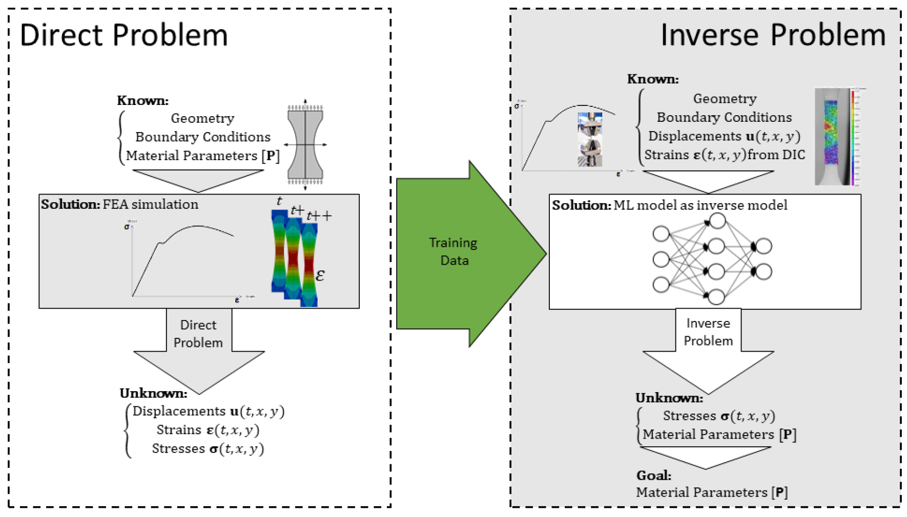
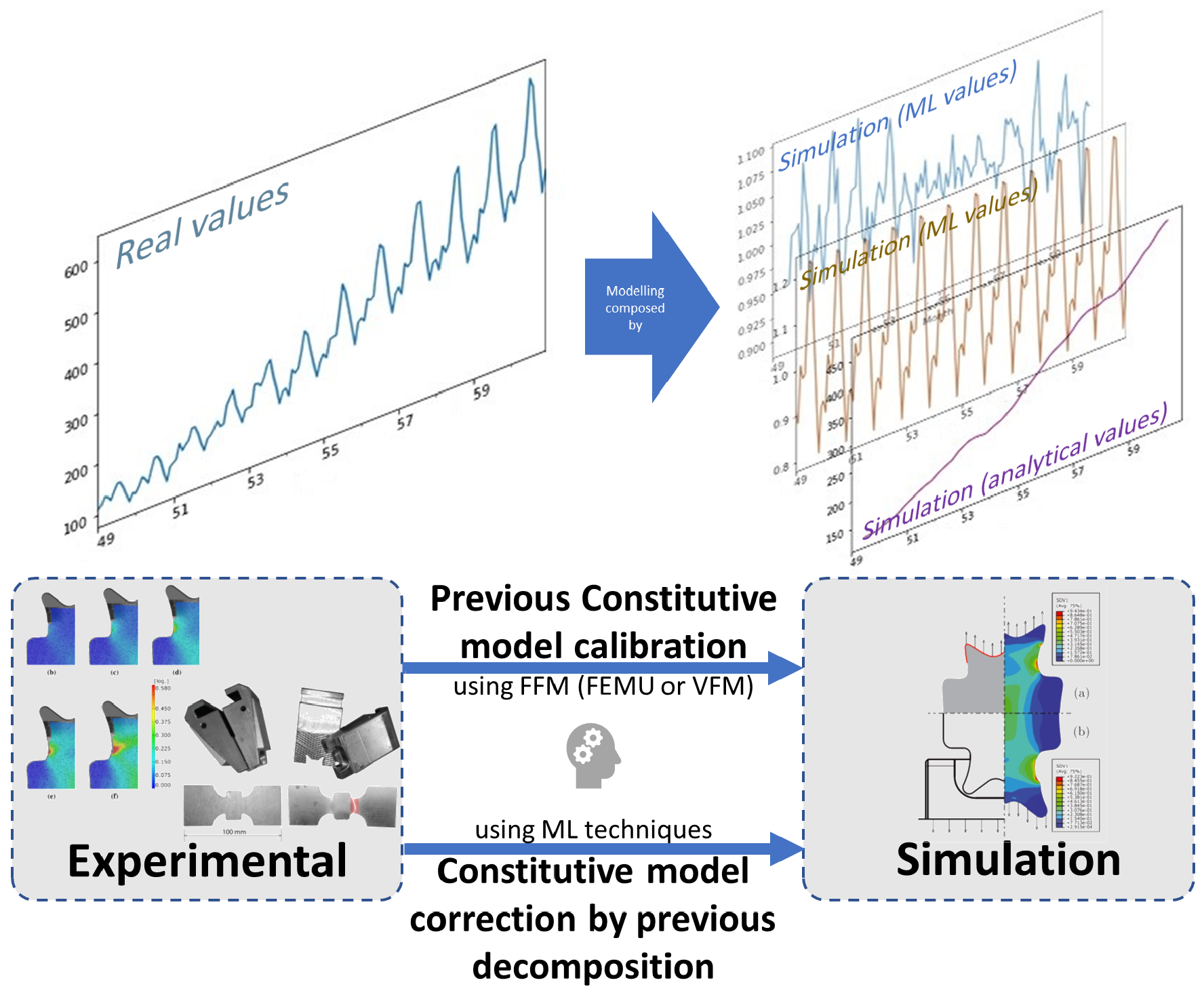
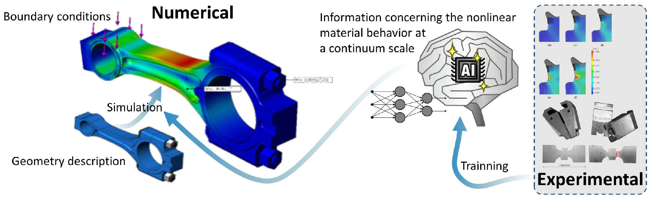
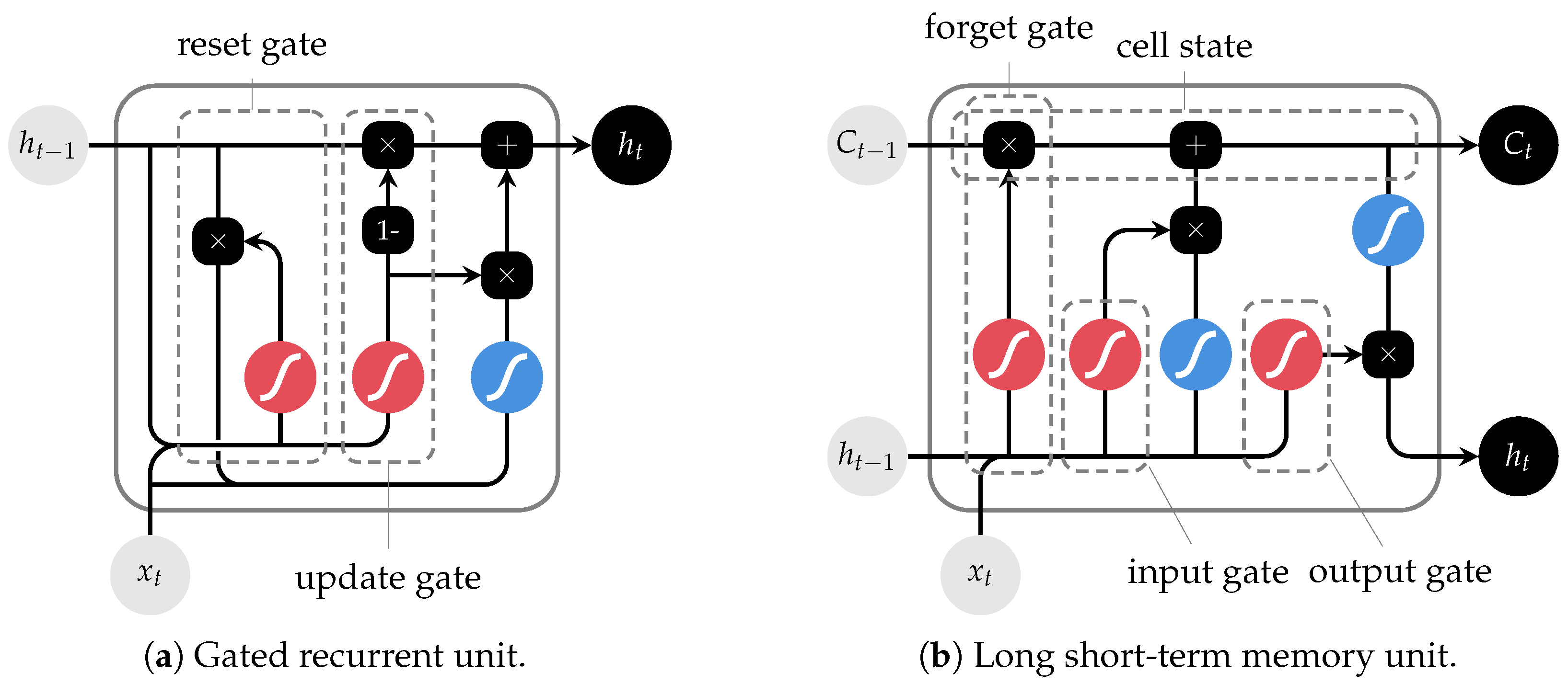
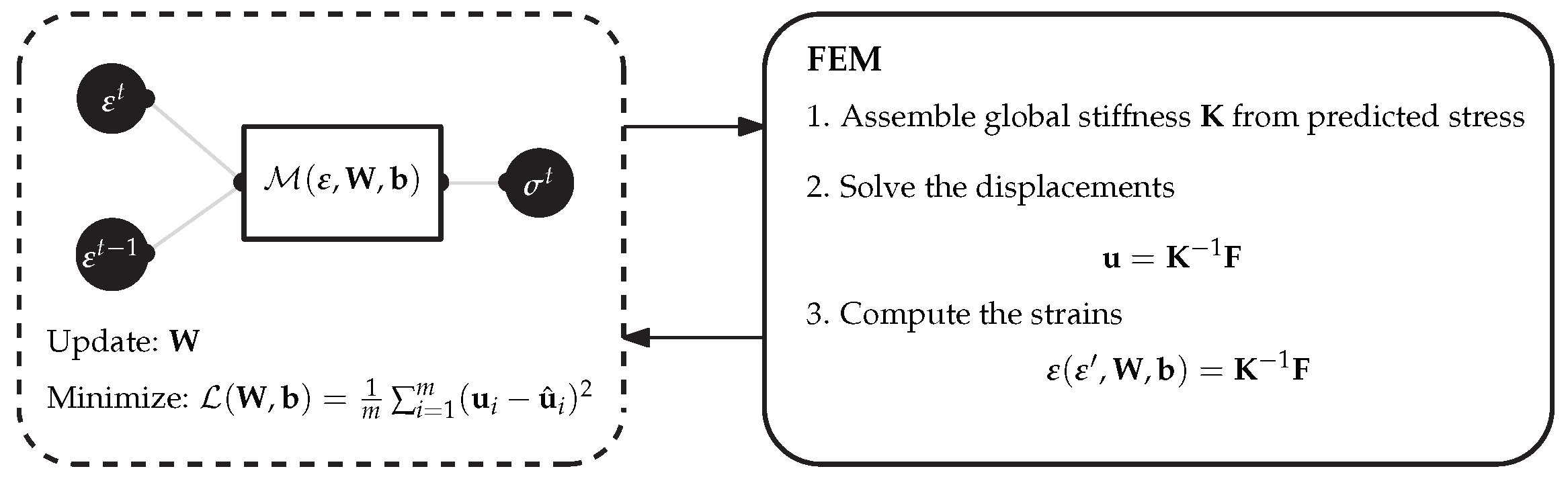
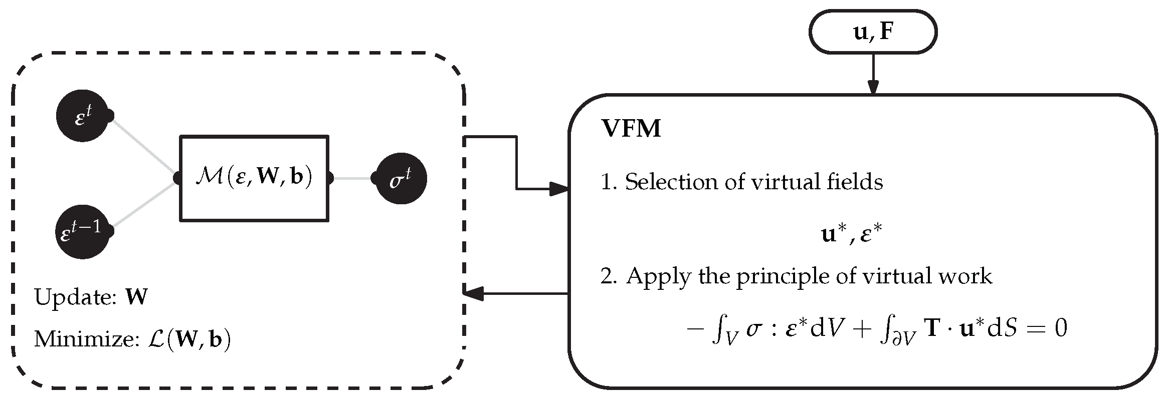
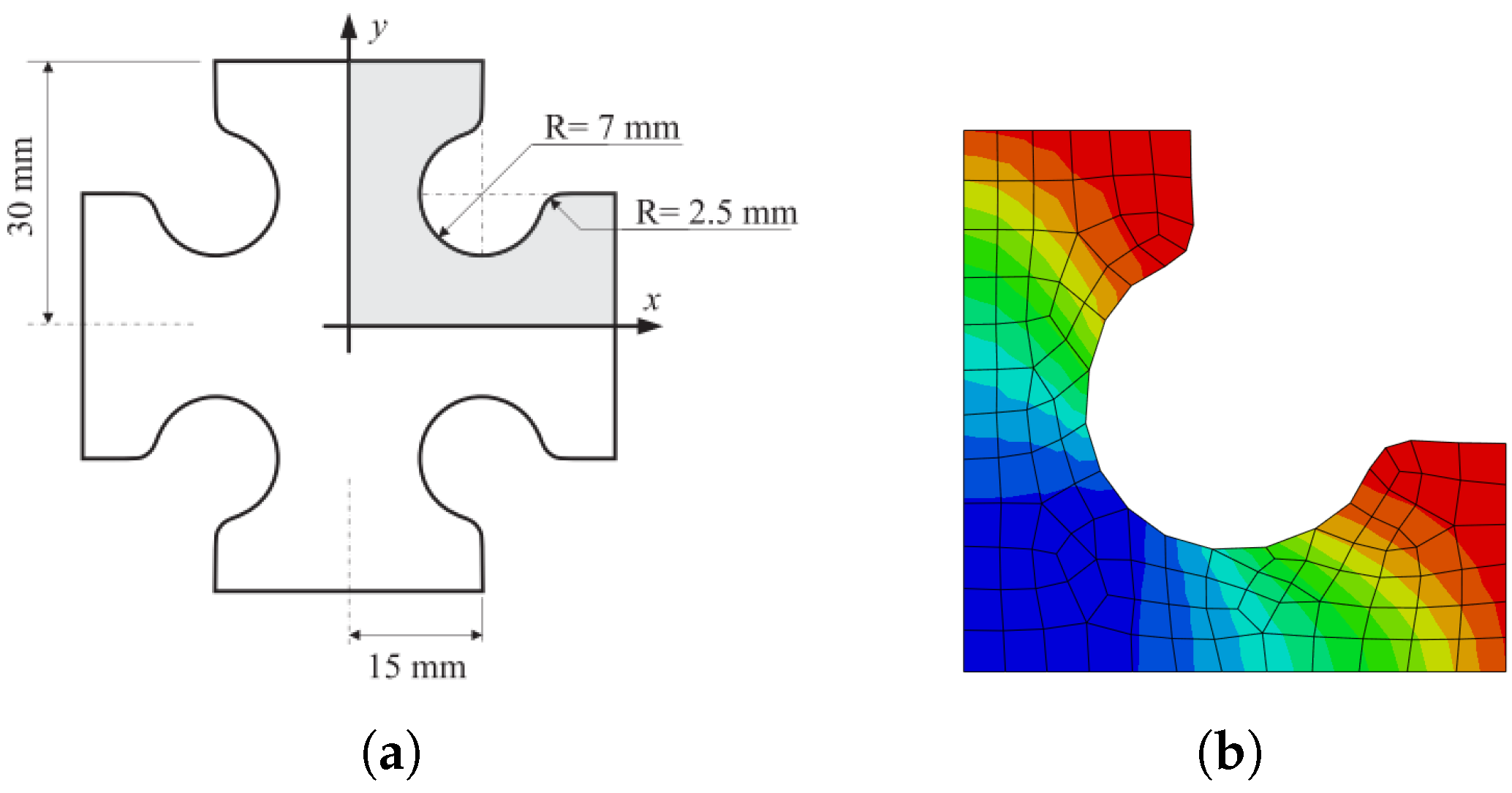
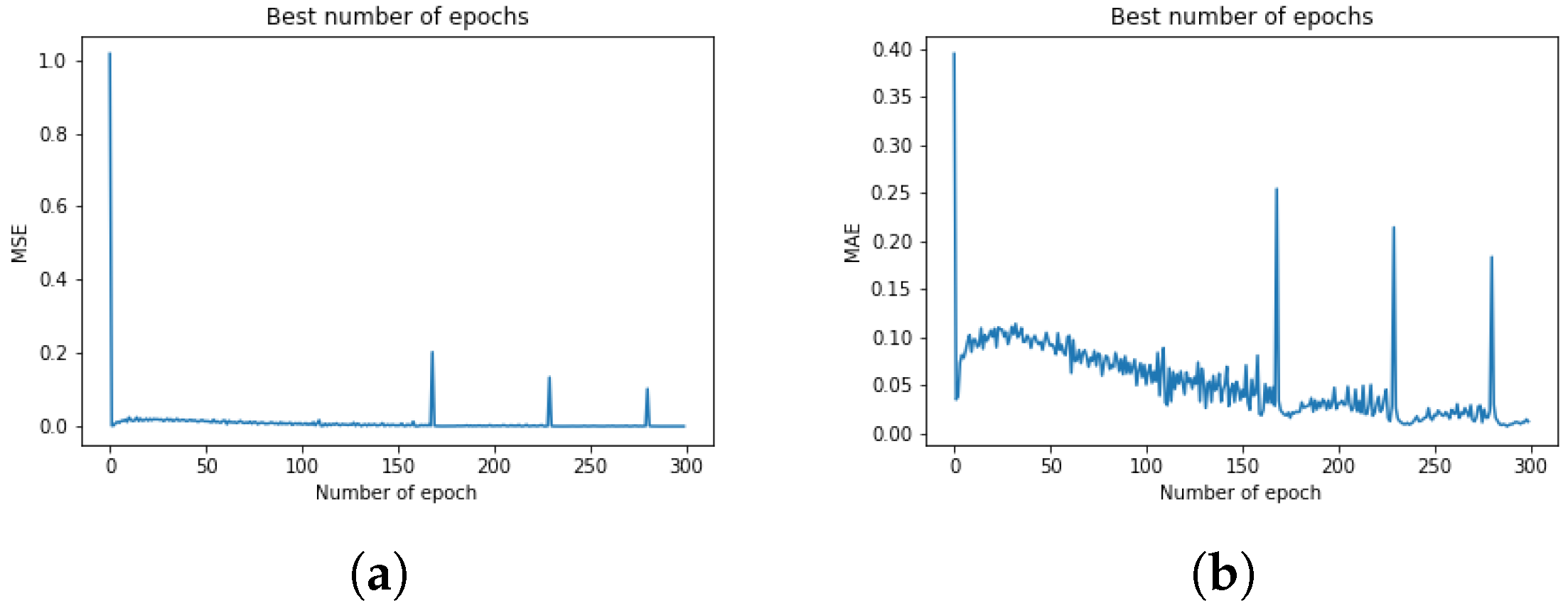
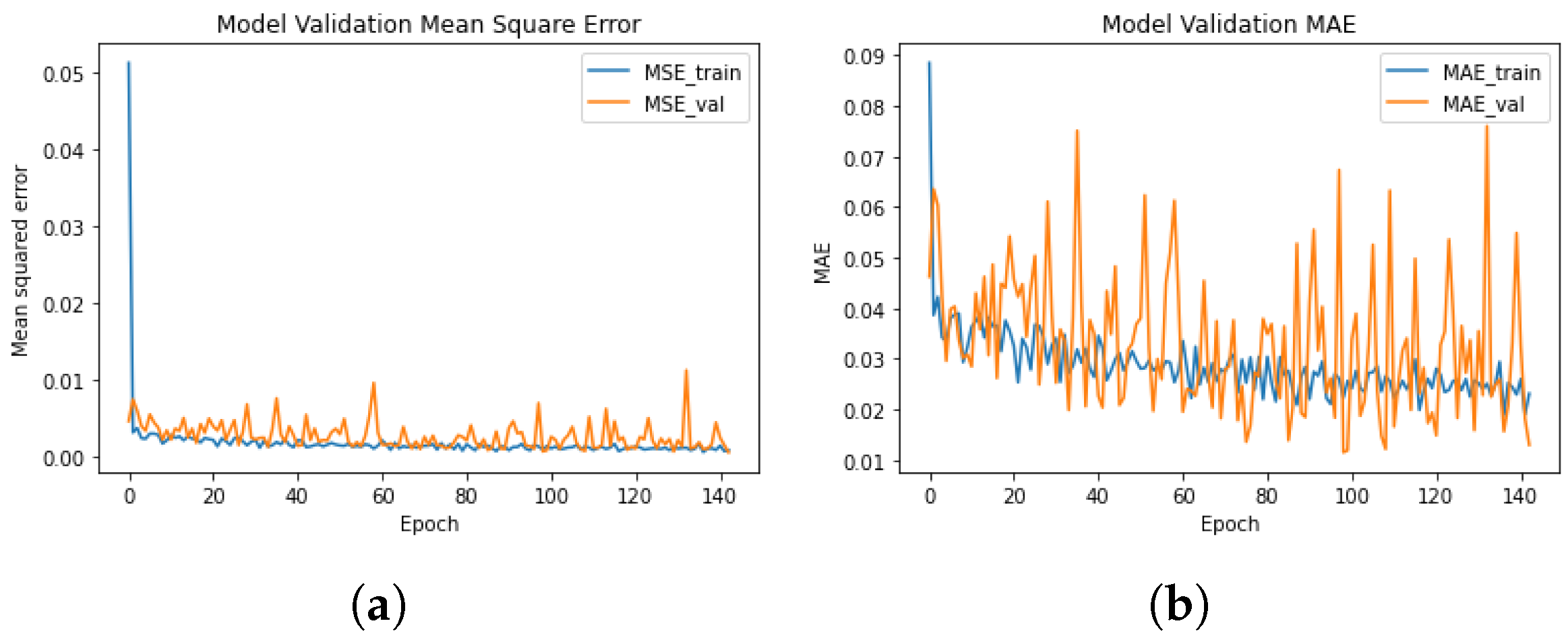
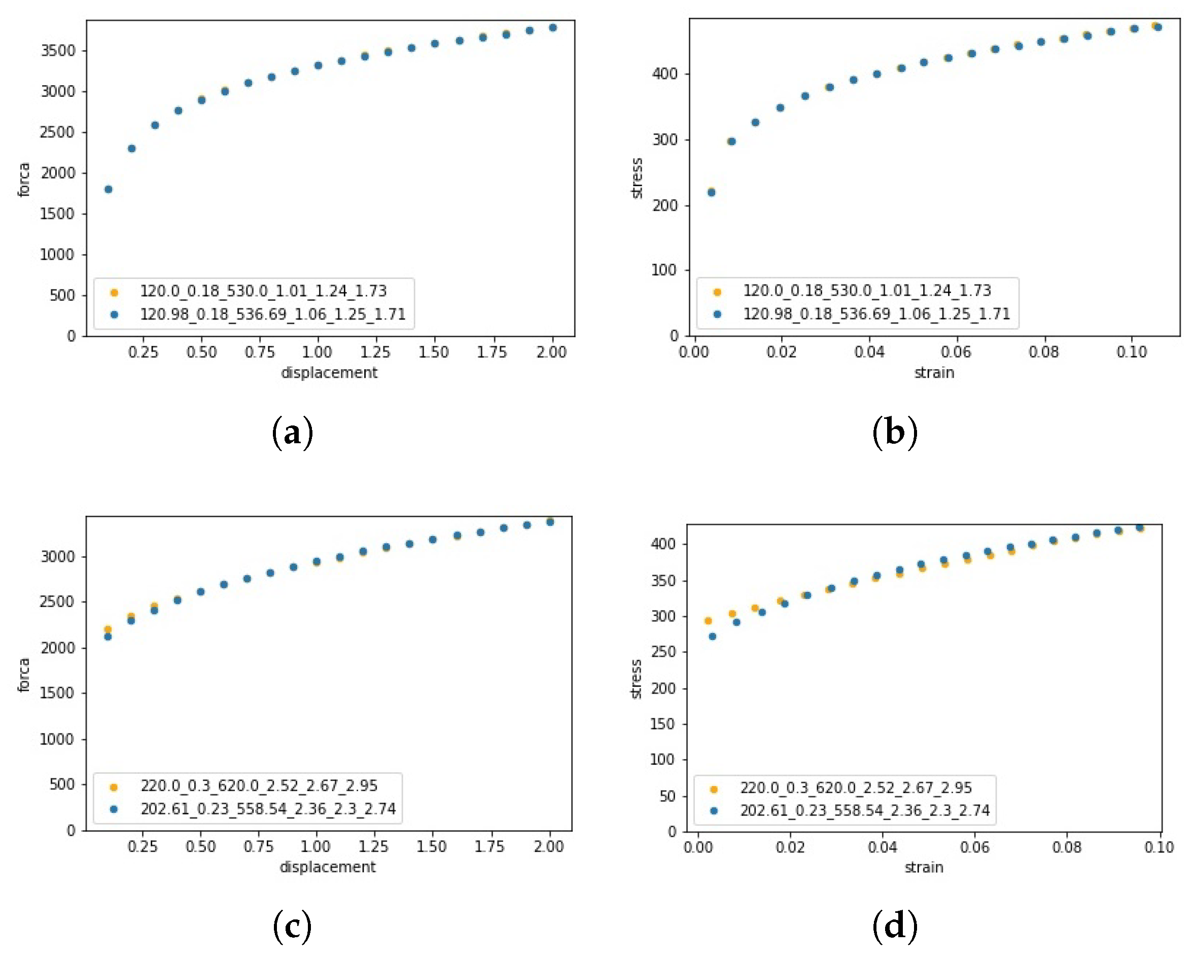
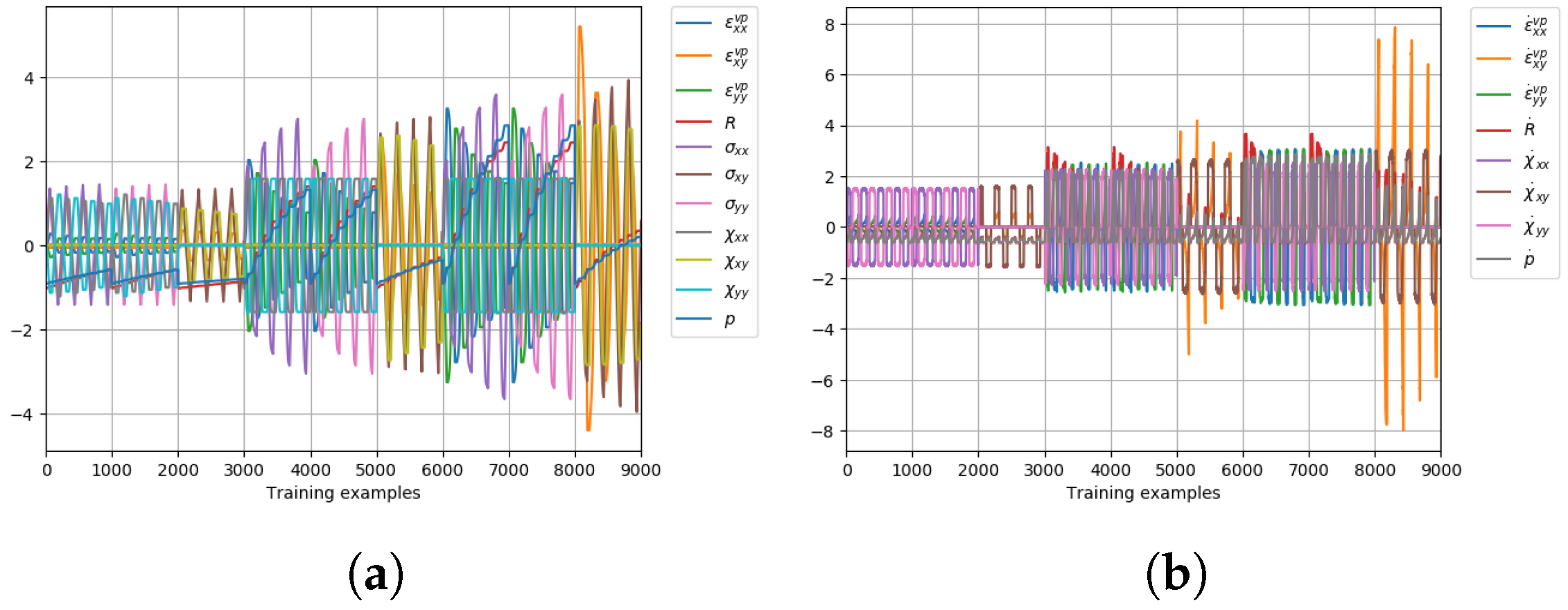
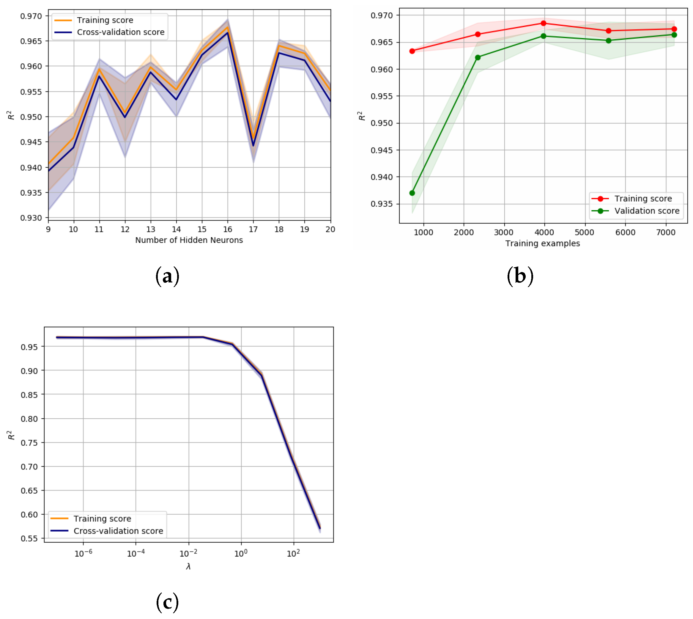
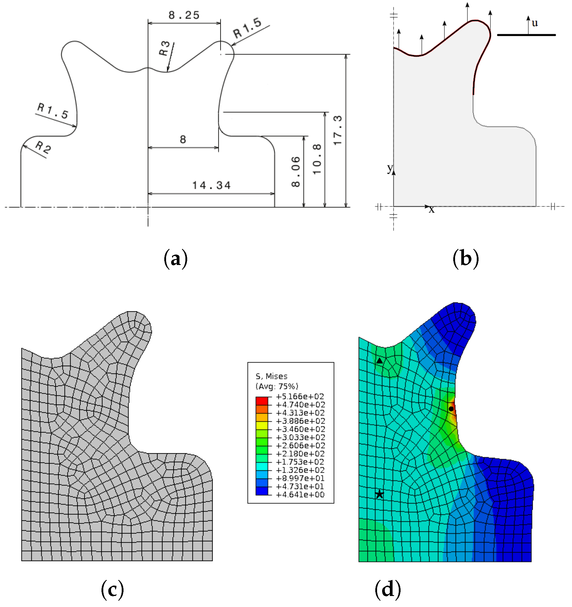
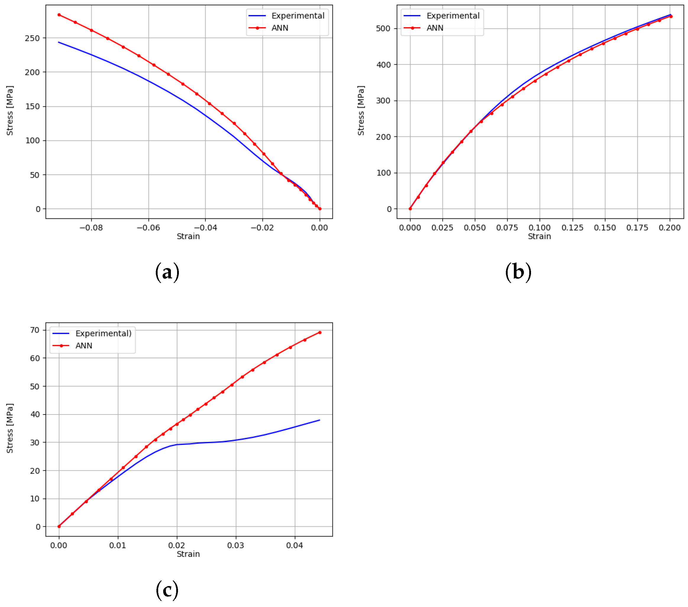
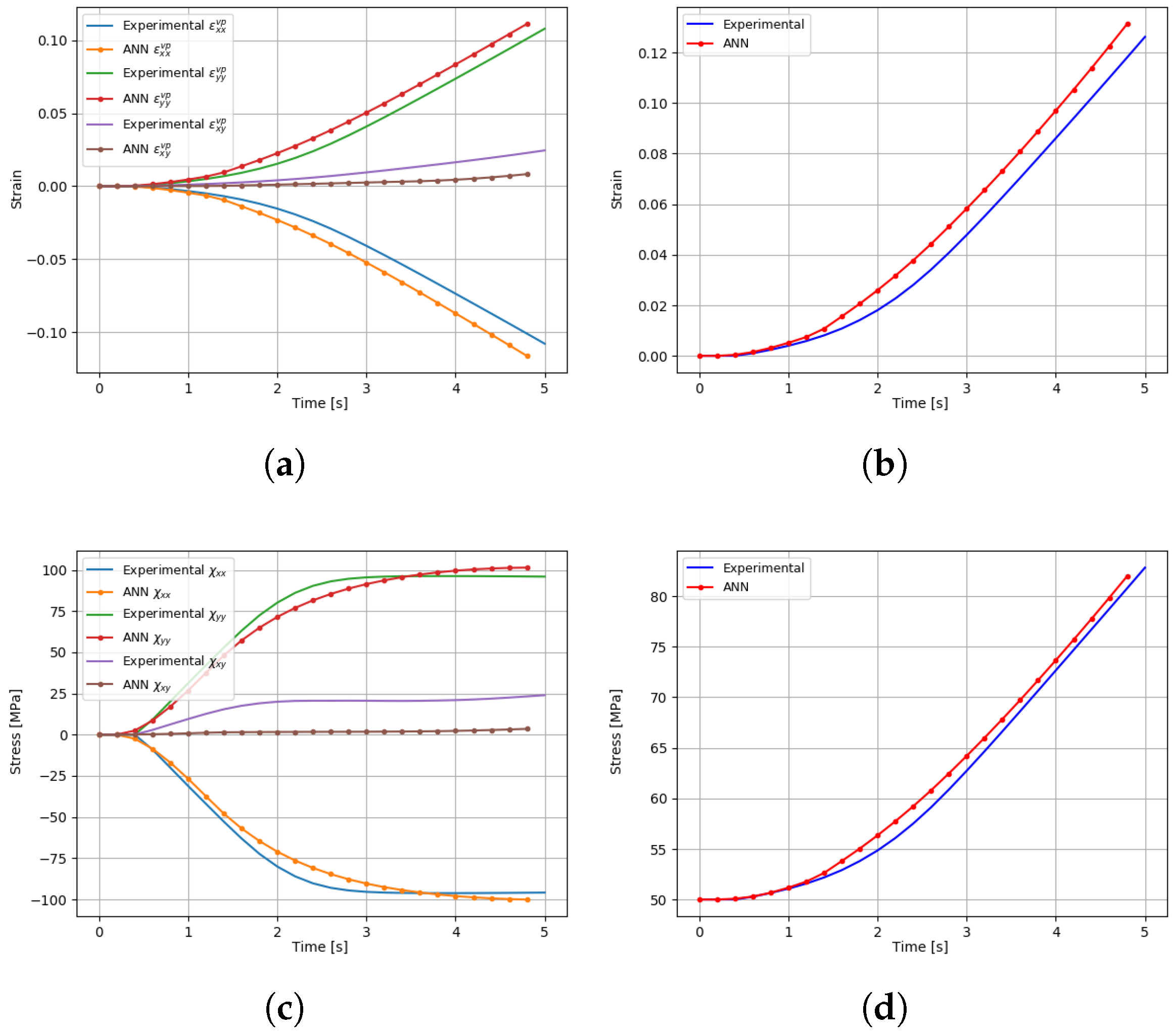
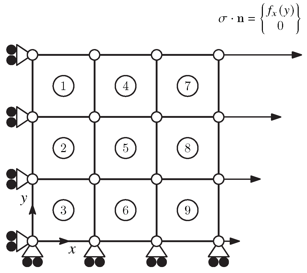
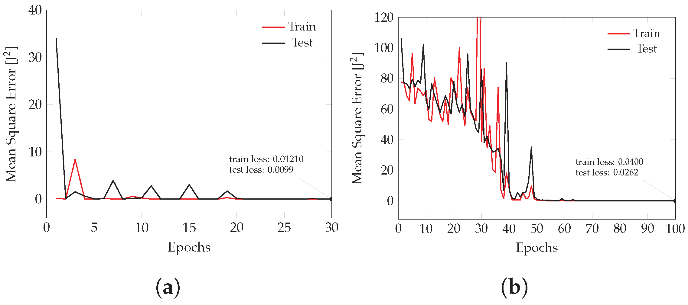
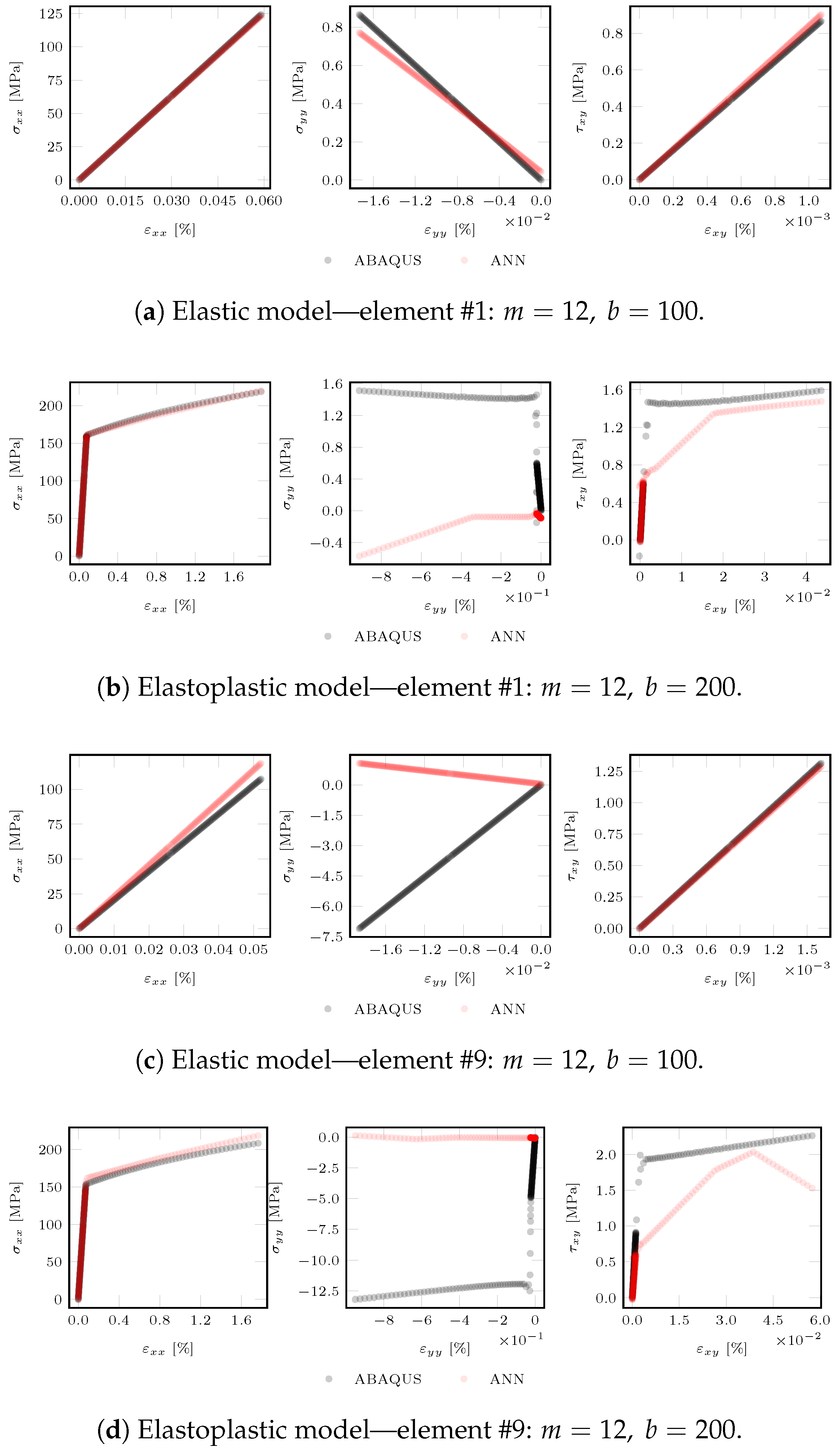
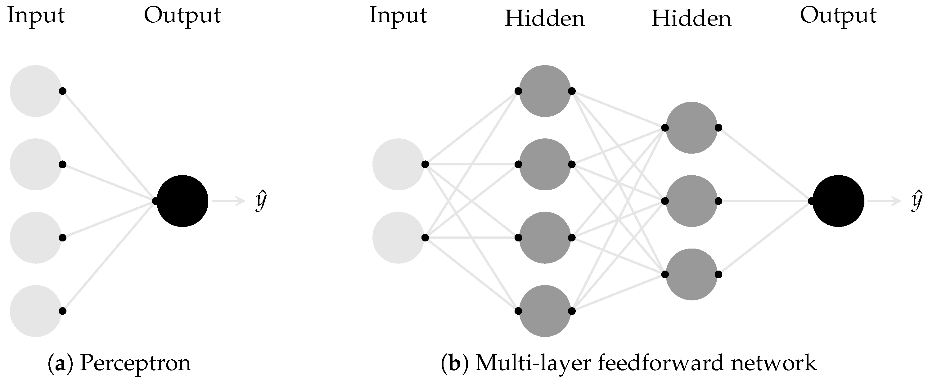
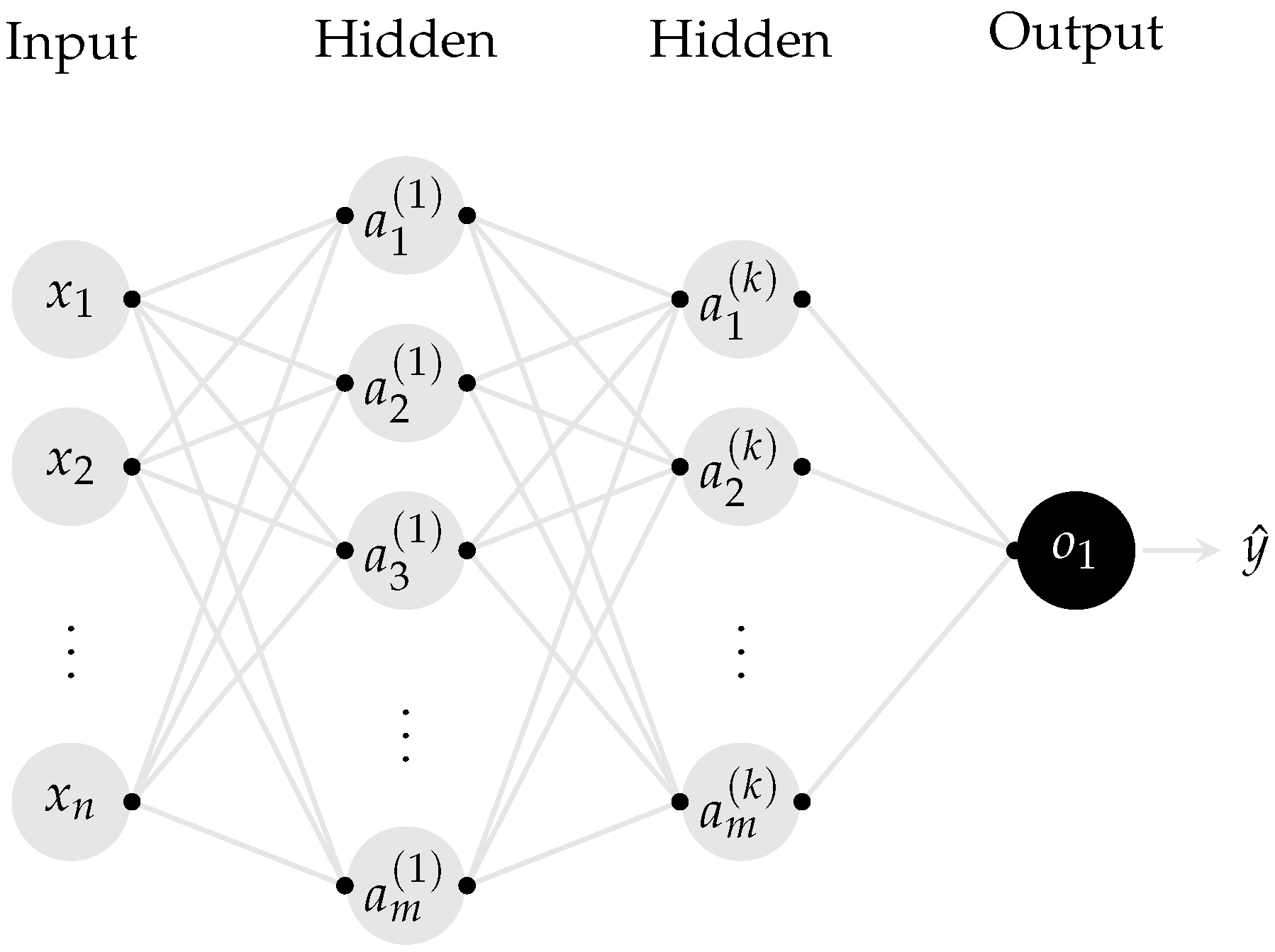
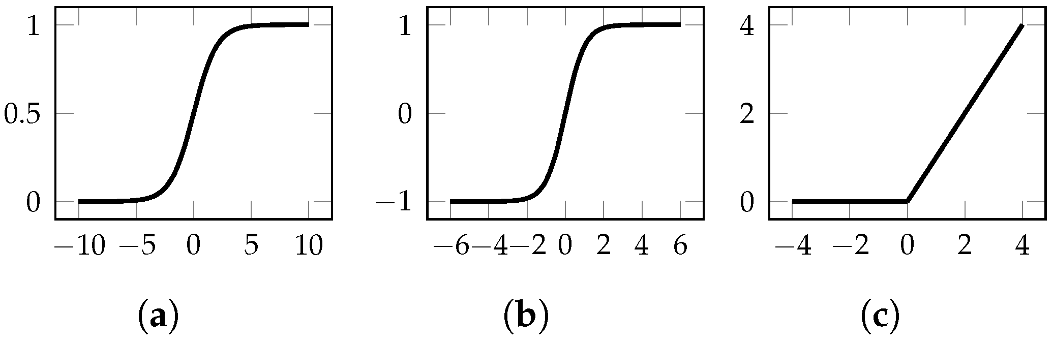
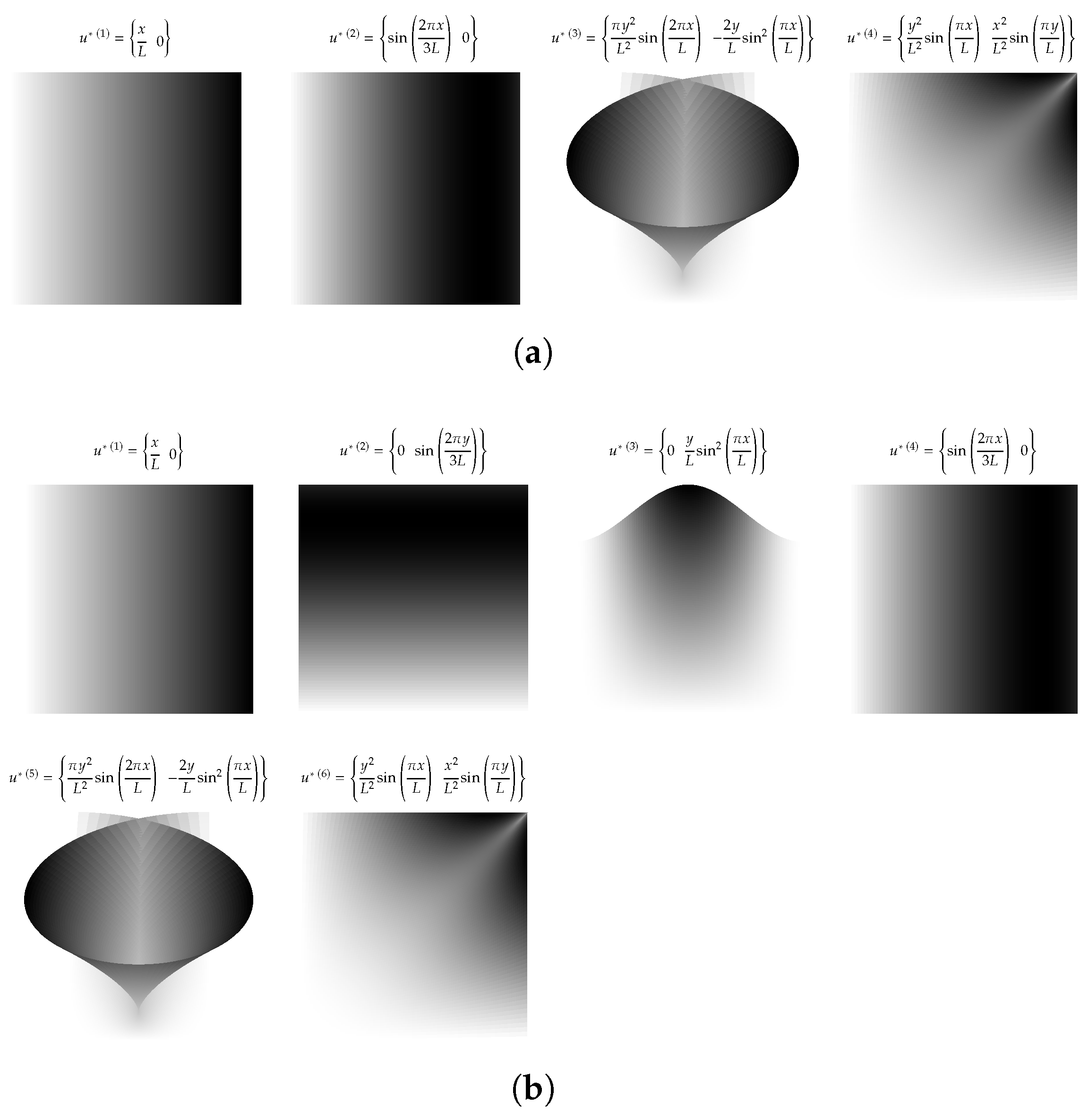
Table 1.
Plastic anisotropy coefficients used for obtaining the reference cruciform biaxial test [63].
Table 1.
Plastic anisotropy coefficients used for obtaining the reference cruciform biaxial test [63].
| Hill’48 Parameters | Reference Values |
|---|---|
| 1.680 | |
| 1.890 | |
| 2.253 |
Table 2.
Input space of constitutive parameters for the biaxial test.
| Constitutive Parameters | Input Space |
|---|---|
| [MPa] | 120–200 |
| n | 0.175–0.275 |
| K [MPa] | 480–570 |
| 1.0–2.5 | |
| 1.0–2.5 | |
| 1.0–2.5 |
Table 3.
ANN architecture for the biaxial test.
| Layer | Neurons | Activation | Kernel_Initializer |
|---|---|---|---|
| Input | 7203 | - | - |
| Dense 1 | 7000 | tanh | Orthogonal |
| Dense 2 | 3000 | tanh | Truncated normal |
| Dense 3 | 5000 | tanh | Truncated normal |
| Dense 4 | 5000 | selu | Variance scaling |
| Dense 5 | 6000 | selu | Variance scaling |
| Output | 6 | - | - |
Table 4.
Predictions and corresponding errors for inverse cruciform test model.
| [MPa] | n | K [MPa] | |||||
|---|---|---|---|---|---|---|---|
| Test 1 | Reference | 120.00 | 0.18 | 530.00 | 1.01 | 1.24 | 1.73 |
| Predicted | 120.98 | 0.18 | 536.69 | 1.06 | 1.25 | 1.71 | |
| Error [%] | 0.82 | 1.67 | 1.26 | 4.95 | 0.81 | 1.16 | |
| Test 2 | Reference | 160.00 | 0.26 | 565.00 | 1.68 | 1.89 | 2.253 |
| Predicted | 160.34 | 0.26 | 565.60 | 1.69 | 1.88 | 2.27 | |
| Error [%] | 0.21 | 1.15 | 0.11 | 0.60 | 0.53 | 0.75 | |
| Test 3 | Reference | 220.00 | 0.30 | 620.00 | 2.52 | 2.67 | 2.95 |
| Predicted | 202.61 | 0.24 | 558.54 | 2.36 | 2.30 | 2.74 | |
| Error [%] | 7.90 | 21.67 | 9.91 | 6.35 | 13.86 | 7.12 |
Table 5.
Comparison of the ANN approach with other approaches presented in [63] for the parameter identification using the biaxial cruciform test for the test case 2.
Table 5.
Comparison of the ANN approach with other approaches presented in [63] for the parameter identification using the biaxial cruciform test for the test case 2.
| [MPa] | n | K [MPa] | |||||
|---|---|---|---|---|---|---|---|
| Reference | 160.00 | 0.26 | 565.00 | 1.68 | 1.89 | 2.25 | |
| ANN approach (96 h) | Predicted | 160.34 | 0.26 | 565.60 | 1.69 | 1.88 | 2.27 |
| Error [%] | 0.21 | 1.15 | 0.11 | 0.60 | 0.53 | 0.75 | |
| VFM (<5 min) | Predicted | 159.76 | 0.26 | 566.16 | 1.67 | 1.91 | 2.24 |
| Error [%] | 0.15 | 0.44 | 0.25 | 0.16 | 1.11 | 0.26 |
Table 6.
Predictions with the ANN inverse cruciform model using the noise-polluted dataset.
| [MPa] | n | K [MPa] | |||||
|---|---|---|---|---|---|---|---|
| Test 1 | Reference | 120.00 | 0.18 | 530.00 | 1.01 | 1.24 | 1.73 |
| Predicted | 146.82 | 0.197 | 568.02 | 1.66 | 1.72 | 1.98 | |
| Error | 22.35 | 9.44 | 7.17 | 64.36 | 38.71 | 14.45 | |
| Test 2 | Reference | 160.00 | 0.26 | 565.00 | 1.68 | 1.89 | 2.25 |
| Predicted | 152.79 | 0.23 | 558.82 | 1.66 | 1.72 | 1.98 | |
| Error | 4.51 | 10.00 | 1.09 | 8.93 | 8.47 | 18.77 | |
| Test 3 | Reference | 220.00 | 0.30 | 620.00 | 2.52 | 2.67 | 2.95 |
| Predicted | 166.61 | 0.23 | 554.62 | 1.77 | 1.73 | 1.93 | |
| Error | 24.27 | 24.27 | 10.55 | 29.76 | 35.21 | 34.58 |
Table 7.
Comparison between the ANN model and the (virtual) experimental values at the end of the butterfly test for selected points: stress comparison [22].
Table 7.
Comparison between the ANN model and the (virtual) experimental values at the end of the butterfly test for selected points: stress comparison [22].
[MPa] | [MPa] | [MPa] | [MPa] | [MPa] | [MPa] | R [MPa] | ||
|---|---|---|---|---|---|---|---|---|
Point 1  | ANN | 283.88 | 533.31 | 69.08 | −100.18 | 101.41 | 3.49 | 81.97 |
| Experiment | 243.42 | 537.35 | 37.83 | −95.94 | 95.94 | 23.94 | 82.81 | |
| Error [%] | 16.62 | 0.75 | 82.61 | 4.42 | 5.7 | 85.42 | 1.01 | |
Point 2  | ANN | −29.96 | 180.21 | 0.96 | −64.34 | 64.08 | 1.72 | 52.49 |
| Experiment | −25.78 | 180.33 | 1.05 | −69.35 | 69.35 | 0.77 | 53.35 | |
| Error [%] | 0.16 | 0.07 | 8.57 | 7.22 | 7.60 | 0.01 | 1.61 | |
Point 3  | ANN | 0.62 | 163.06 | 7.47 | −48.62 | 48.28 | 1.25 | 51.80 |
| Experiment | −0.66 | 168.67 | 6.61 | −52.11 | 52.11 | 4.18 | 52.07 | |
| Error [%] | 193.94 | 3.33 | 13.01 | 6.7 | 7.35 | 70.1 | 0.52 |
Table 8.
Comparison between the ANN model and the (virtual) experimental values at the end of the butterfly test for selected points: strain comparison [22].
Table 8.
Comparison between the ANN model and the (virtual) experimental values at the end of the butterfly test for selected points: strain comparison [22].
| p | |||||
|---|---|---|---|---|---|
Point 1  | ANN | −1.162 | 1.111 | 8.266 | 1.313 |
| Experiment | −1.079 | 1.079 | 2.452 | 1.262 | |
| Error [%] | 7.69 | 2.97 | 66.29 | 4.04 | |
Point 2  | ANN | −9.948 | 1.055 | 1.798 | 1.162 |
| Experiment | −1.077 | 1.077 | 1.400 | 1.244 | |
| Error [%] | 7.63 | 2.04 | 28.43 | 6.59 | |
Point 3  | ANN | −7.230 | 7.836 | 9.220 | 8.538 |
| Experiment | −6.630 | 6.630 | 5.400 | 7.670 | |
| Error [%] | 9.05 | 18.19 | 82.93 | 11.32 |
Table 9.
Virtual fields used to train both ANN models. Virtual fields 1 through 4 were used to train the elastic model, while the whole set was used to trained the elastoplastic model.
Table 9.
Virtual fields used to train both ANN models. Virtual fields 1 through 4 were used to train the elastic model, while the whole set was used to trained the elastoplastic model.
| Virtual Field | 1 | 2 | 3 | 4 | 5 | 6 |
|---|---|---|---|---|---|---|
| 0 | 0 | |||||
| 0 | 0 | |||||
| 0 | 0 | |||||
| 0 | 0 | |||||
| 0 | 0 | 0 | 0 |
Publisher’s Note: MDPI stays neutral with regard to jurisdictional claims in published maps and institutional affiliations. |
© 2022 by the authors. Licensee MDPI, Basel, Switzerland. This article is an open access article distributed under the terms and conditions of the Creative Commons Attribution (CC BY) license (https://creativecommons.org/licenses/by/4.0/).
Share and Cite
MDPI and ACS Style
Lourenço, R.; Andrade-Campos, A.; Georgieva, P. The Use of Machine-Learning Techniques in Material Constitutive Modelling for Metal Forming Processes. Metals 2022, 12, 427. https://0-doi-org.brum.beds.ac.uk/10.3390/met12030427
AMA Style
Lourenço R, Andrade-Campos A, Georgieva P. The Use of Machine-Learning Techniques in Material Constitutive Modelling for Metal Forming Processes. Metals. 2022; 12(3):427. https://0-doi-org.brum.beds.ac.uk/10.3390/met12030427
Chicago/Turabian StyleLourenço, Rúben, António Andrade-Campos, and Pétia Georgieva. 2022. "The Use of Machine-Learning Techniques in Material Constitutive Modelling for Metal Forming Processes" Metals 12, no. 3: 427. https://0-doi-org.brum.beds.ac.uk/10.3390/met12030427
Note that from the first issue of 2016, this journal uses article numbers instead of page numbers. See further details here.