Research on Normal Contact Stiffness of Rough Joint Surfaces Machined by Turning and Grinding

Abstract

In order to accurately obtain the contact stiffness of rough joint surfaces machined by turning and grinding, a research simulation is carried out by using the finite element method. Based on the surface modeling method under the combined machining mode, the three-dimensional (3D) solid model is constructed. Then, the finite element results of the normal contact stiffness were obtained through contact analysis. The comparative analysis was carried out with the analytical results of the KE model and the experimental results. The comparison results show that three results have the same trend of change. However, the maximum relative error of the finite element results is 6.03%, while that of the analytical results for the KE model is 60.07%. After that, the finite element results under different machining parameters are compared. The normal contact stiffness increases with the increase in the turning tool arc radius, grinding depth, and fractal dimension, but decreases with the increase in the turning feed rate and scale coefficient. The rationality of the results is explained by the distribution of the asperities and the contact deformation law of the asperities on the rough surface.

1. Introduction

The normal contact stiffness is the key parameter to describe the contact characteristics of mechanical joint surfaces and directly affects the connection performance of mechanical parts [1,2]. In practice, due to the lack of accurate normal contact stiffness parameters, it is difficult to carry out the design of the mechanical structure for precision equipment. How to accurately and effectively obtain the normal contact stiffness of mechanical joint surfaces has become an urgent problem to be solved [3,4].

The normal contact stiffness of rough interfaces has always been an important topic in the field of tribology [1,5]. The research on normal contact stiffness can be traced back to the 1960s [6]. In terms of the different shapes of asperities, Greenwood and Williamson first proposed an analytical model of contact stiffness (GW model) [7] based on the assumption of hemispherical asperities. Bush used a parabola to simulate the profile of asperities on the rough surface and studied the normal contact stiffness of the rough joint surface based on the parabolic asperities [8]. Komvopoulos regarded the asperities on the machined surface as cylindrical and studied the normal contact stiffness of the rough joint based on the cylindrical asperities [9]. Horng extended the GW model in combination with semi-elliptical asperities and established a normal contact stiffness model based on semi-elliptical asperities [10]. An fitted the measured shape of asperities on rough surfaces and proposed a normal contact stiffness model based on sinusoidal asperities [11]. In terms of the contact deformation of the asperities, the asperities will undergo three processes of elastic, elastic–plastic, and plastic deformation during the compression deformation process. Chang considered elastic–plastic contact based on the volume conservation theory of plastic deformation, and then established the contact model (CEB model) [12]. Zhao used the template function to realize the transition from elastic deformation to plastic deformation of asperity and proposed the contact model (ZMC model) considering elastic, elastic–plastic, and plastic deformation [13,14]. Ciavarella introduced the interaction of asperities on rough surfaces into the theoretical analytical model and improved the previous GW model [15].

With the development of finite element technology, Kogut used the finite element method to analyze the contact between the hemisphere and the rigid plane. The empirical formula of the contact parameters changing with the indentation depth is obtained, and the finite element contact model (KE model) of the rough surface is established [16]. Based on the KE model, Chandrasekar considered the interaction of asperities in the deformation process of asperities and proposed a KE model considering the interaction of asperities [17]. After that, a simple contact model in which the mechanical bonding surfaces are close to complete contact was proposed [18]. Gao introduced the lateral contact problem of asperities into the KE model and established a contact stiffness model considering the contact angle of asperities [19]. In the process of establishing the contact stiffness model, Li combined the continuous smoothness of asperities on rough surfaces with the interaction of asperities [5].

The above research seems to be more inclined to research on the general contact model of rough joint surfaces, and the research process is not related to the processing method and processing parameters. The general model may not be able to meet the calculation accuracy for the contact stiffness, resulting in a deviation between the theoretical and experimental results. This fact has also been confirmed in the ultrasonic reflection coefficient experiments [20] and digital image correlation (DIC) experiments [21]. In addition, the deformation law of asperities on rough surfaces is more complicated. Due to the lack of a contact mechanics theory, there is no accurate and recognized analytical formula for the normal contact stiffness of rough joint surfaces. More importantly, the above research results cannot form guiding recommendations for the machining process.

The quality of the machined surface is the fundamental reason that affects the connection characteristics of the mechanical joint surface. The study of machining parameters and surface roughness can make people better understand the formation mechanism of rough surfaces, which is of great significance to the study of contact parameters of rough joint surfaces. The development of micro-measurement technology provides a basis for the research on the relationship between machining methods and the roughness of the machined surface. Yazman studied the effect of cutting speeds on the macrostructure, microstructure, and work hardening of as-cast and isothermal-quenched ductile iron chips [22]. Subsequently, Yazman discussed the influence of cold chamber die casting parameters on the machinability of AZ91 magnesium alloy high-speed drilling through experimental research [23,24]. Uludağ changed the microstructure of the Al–7Si alloy by adding AlSr15, AlTi5B1, and Al3B, and discussed the correlation between the bifilm index and the surface roughness of machined parts [25]. Aamir investigated the effects of uncoated tools and four tool coatings (TiN-, TiCN-, TiAlN-, and TiSiN) on hole quality and the microstructure [26]. The above research was based on the actual machining parameters and materials, and the research results have a guiding role for actual machining and have important engineering value.

Based on the above research, two issues seem to be overlooked. Firstly, most researchers seem to be limited to research on the normal contact stiffness of rough joint surfaces under a single processing mode. Secondly, the contact stiffness calculation results are not linked to the actual machining parameters. Both of the above issues will lead to discrepancies between analytical and experimental results. Therefore, based on the surface topography obtained by the machining parameters, the normal contact stiffness of rough joint surfaces machined by turning and grinding is calculated by the finite element method. Meanwhile, the variation law of the normal contact stiffness of rough joint surfaces with machining parameters will be explored, which has guiding significance for machining production.

2. Surface Modeling Method under the Combined Machining Mode

2.1. Turning Mode

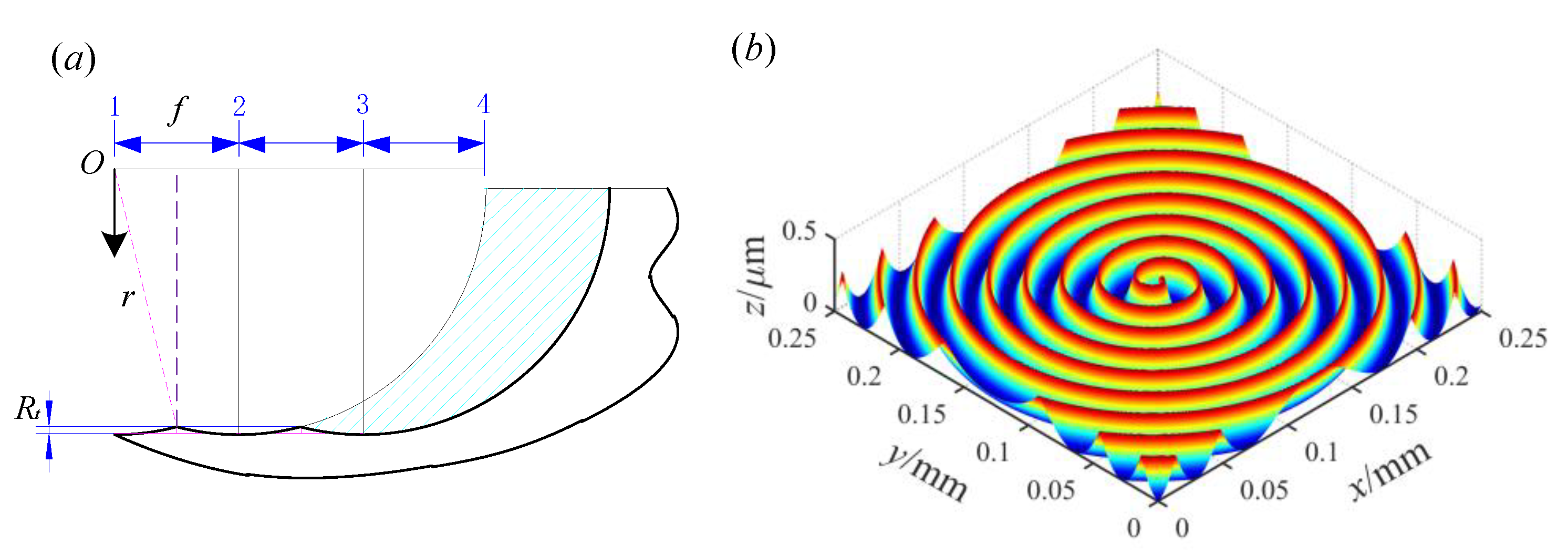
The shape of the tool used in turning mode is regular, and the topography of the turning surface can be constructed based on the principle of turning kinematics [27]. It is worth noting that the turning surface topography is produced under longitudinal turning conditions. Figure 1a shows the schematic diagram of the modeling of the surface topography under turning mode based on the principle of turning kinematics. Suppose that the turning tool arc radius is r and the turning feed rate is f. As can be seen from Figure 1a, during the turning process, the turning tool and the work-piece move relative to each other, and the turning tool will remove the surface material of the work-piece.

With the rotation of the work-piece, the corresponding turning profile is left on the surface of the work-piece. The maximum height of the profile is defined as the residual height R_t. From the geometric relationship, the relationship between the residual height R_t, the turning tool arc radius r, and the feed rate f can be obtained, as shown in Equation (1).

$$R_t=r-\sqrt{r^2-f^2/4}$$

(1)

Based on the above analysis, when the arc radius and the turning feed rate are set, the turning surface’s topography can be determined. The formation process of the 3D topography of turning surfaces is introduced in detail in references [27,28], which will not be repeated here. According to the surface modeling process described in the literature, the 3D topography of turning surfaces can be constructed by using MATLAB software (R2018b, MathWorks, Natick, MA, USA). The 3D topography under the condition of r = 0.2 mm and f = 0.2 mm/r is shown in Figure 1b. The plan view of the measured topography for the turning surface and the 3D topography of the measured turning surface can be found in Figure S1. Since the contact pressure in the final result is within the unit area, the area of the 3D topography has no effect on the result. Considering the running efficiency and cost of the simulation software, the area of the 3D topography is taken as 0.25 mm × 0.25 mm, and this size is applicable to the following topography display graphics.

2.2. Grinding Mode

Different from the tools used in cutting, the formation of the topography of the grinding surface is essentially different from the turning mode. The shape of abrasive grains on the grinding wheel is disordered and irregular, so the construction process of the grinding surface is more complex. Aiming at this problem, fractal surfaces can well satisfy the complex topography of grinding surfaces [29]. Moreover, the relevant literature also confirmed that using a fractal surface to simulate a grinding surface has the advantage of fewer errors compared to other surfaces [30]. Therefore, the 3D fractal surface is used to simulate the grinding surface in this paper. The 3D fractal surface was proposed by Yan and Komvopoulos [31], and the functional expression of the 3D fractal surface was given in the literature, as shown in Equation (2).

$$\begin{array}{l}z\left(x,y\right)=L\cdot {\left(\frac{G}{L}\right)}^{D_s-2}\cdot {\left(\frac{\ln \gamma }{M}\right)}^{1/2}\cdot \\ {\displaystyle \sum _{m=1}^M{\displaystyle \sum _{n=0}^{n_{\max }}\left\{{\gamma }^{\left(D_s-3\right)n}\times \left[\cos {\varphi }_{m,n}-\cos \left(\frac{2\mathsf{\pi }{\gamma }^n{\left(x^2+y^2\right)}^{1/2}}{L}\times \cos \left(\arctan \left(\frac{y}{x}\right)-\frac{\mathsf{\pi }m}{M}\right)+{\varphi }_{m,n}\right)\right]\right\}}}\end{array}$$

(2)

where z is the vertical height of the fractal surface, x and y are the coordinates of the data points in the X and Y directions, respectively, D_s is the fractal dimension of the fractal surface and 2 < D_s < 3, G is the scale coefficient of the fractal surface, γ is the frequency density parameter of fractal surface and γ > 1, L is the sampling length of the fractal surface, M is the number of overlapping wrinkles on the fractal surface, m and n are random phases, the value range is [0, 2π], n_l is the minimum frequency, usually n_l = 0, n_max is the maximum frequency and n_max = int[log(L/L_s)/log γ], L_s is the cut-off length, and φ_m,n is the initial phase.

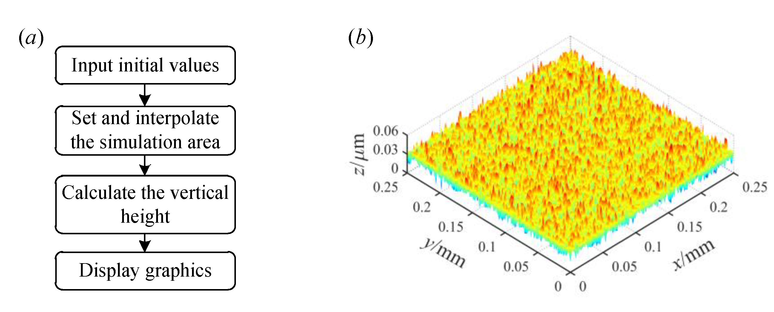
Based on Equation (2), the construction of the 3D fractal surface can be realized by programming with MatlabR2018b software. The 3D fractal surface simulation process is shown in Figure 2a.

The modeling process of the 3D fractal surface can be divided into the following four steps. Firstly, the initial values of the simulation needs to be inputted: the initial values are M = 10, γ = 1.5, L = 1 × 10⁻³ m, L_s = 5 × 10⁻⁹ m, D = 2.5, G = 10⁻⁸, and φ_m,n = π/6, respectively [31]. Secondly, the simulation area is set and interpolated. 256 × 256 interpolation is performed on the simulation area in this paper, and the data after interpolation are taken as the x and y coordinate values. The next step is to use m and n as loop variables to calculate the vertical height z of the fractal surface. Through the above process, the topography of the 3D fractal surface can be obtained. Finally, the vertical height under the corresponding coordinates is displayed graphically. Figure 2b shows the 3D fractal surface under D = 2.5 and G = 10⁻⁸. The plan view of the measured topography for the grinding surface and the 3D topography of the measured grinding surface can be found in Figure S1.

2.3. Combined Machining Mode

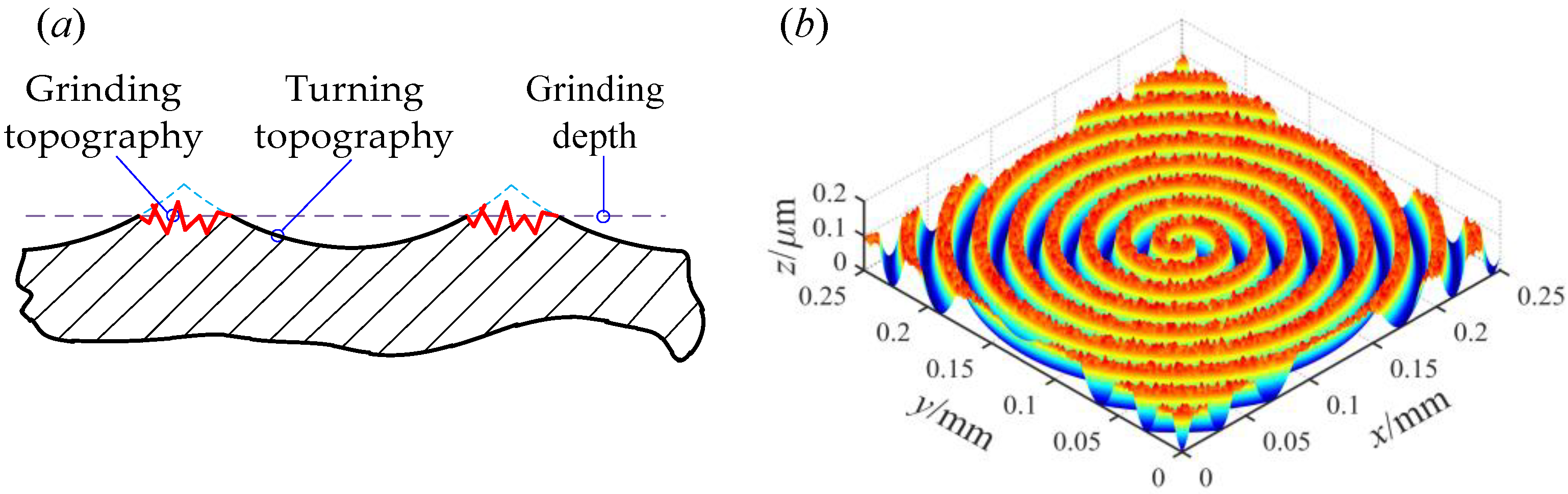
Combined machining mode refers to a single work-piece that has undergone two machining processes. Turning and grinding are two commonly used combined machining modes. During actual machining, for large machining allowances, the turning method can remove surface material faster. However, it is difficult for a single turning method to meet the high surface quality. The combined machining method of turning and grinding can improve the efficiency of machining and meet the needs of higher surface quality. The surface modeling method under the combined machining mode is described below. Figure 3a shows the two-dimensional (2D) topography under the combined machining mode.

It can be seen from Figure 3a that the combined machining topography is a secondary grinding of the surface asperities on the basis of the original turning topography. Based on the cutting theory, during the secondary grinding process of the turning surface, the top area of the residual height of the turning surface will be cut off by the abrasive grains of the grinding wheel. That is, the secondary grinding process will leave the grinding topography on the top area of the original turning topography.

It should be noted that the combined machining mode involves the problem of grinding depth. In order to facilitate the comparison of the normal contact stiffness under different grinding depths, the parameter of the grinding depth ratio (δ_d) is defined. The δ_d is defined as the ratio of the grinding depth to the turning residual height R_t. The grinding depth coincides with the base height of the fractal surface, as shown by the dotted line in Figure 3a.

In the process of secondary grinding of the turning surface, not all the abrasive grains of the grinding wheel are involved in the grinding. For the part involved in grinding, the profile height of the grinding topography will be lower than the turning residual height. For the part not involved in grinding, the profile height of the grinding topography will be higher than the turning residual height.

Therefore, combining the turning topography, the grinding topography, and the grinding depth ratio (δ_d), the 3D surface topography under the combined machining mode can be obtained, as shown in Figure 3b. It can be seen from Figure 3b that after the work-piece has undergone two machining processes, the asperities on the original turning surface will be cut by the abrasive grains of the grinding wheel. Through this combined machining mode, the number of asperities on the surface can be increased, and the distribution of asperities can be more dispersed. Further, the purpose of reducing the surface roughness and improving the surface processing quality can be achieved.

3. Finite Element Contact Simulation

Based on the analysis in Section 2, the 3D topography under the combined machining mode can be obtained. Meanwhile, the point cloud data of the surface topography can be obtained. In this section, the inverse modeling method is used to realize the construction of the point cloud data into to a 3D solid model. Then, the contact analysis of the 3D model is carried out using the finite element method.

3.1. Construction of 3D Solid Model

The 3D solid model is the basis of finite element simulation. Based on the method described in Section 2, the point cloud data of the surface topography can be obtained. The modeling method of the 3D solid model based on the point cloud data will be introduced in this section. The modeling method based on point cloud data is also called inverse modeling, which is widely used in the field of construction machinery [32,33]. In this paper, this method is introduced into a 3D solid model.

The 3D solid model based on point cloud data is different from the modeling of traditional macroscopic objects. For rough surfaces, the microscopic topography has the characteristics of many detailed features and complex feature structures. The accuracy of the model is the basis to ensure the accuracy of the finite element results. Because of the poor modeling accuracy of finite element simulation software, other professional software is required for the modeling process.

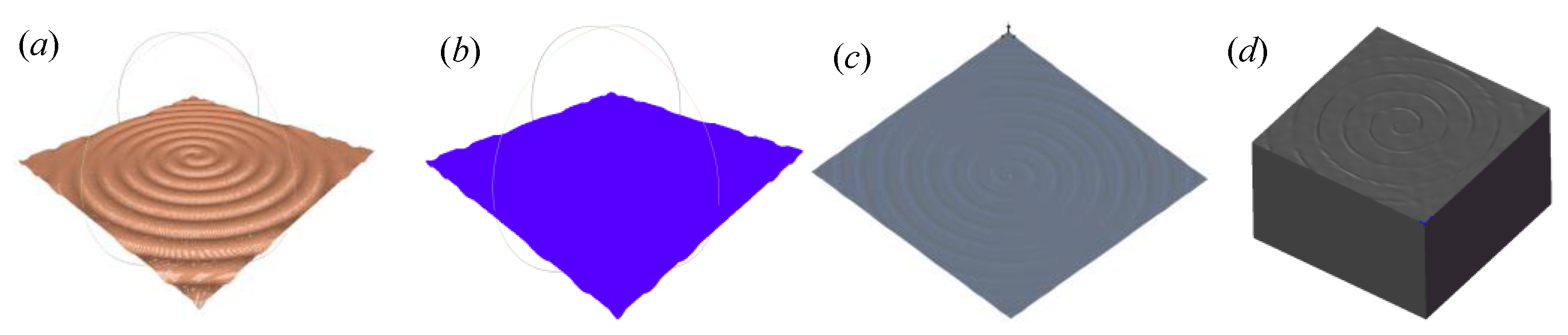
The following is the modeling method of the 3D solid model based on point cloud data. Firstly, the point cloud data needs to be converted into a mesh file. Import the 3D topography point cloud data in the format .stl into the Meshlab software (2016, University of Pisa, Tuscany, Italy). Then, the point cloud data was converted into a mesh file in .ply format. In the process of creating the mesh file, the normal values of the point cloud data point set need to be calculated. After that, the rolling ball method is used to convert the point cloud data into a mesh file. Secondly, the mesh file needs to be converted into a 3D solid model. Import the obtained mesh file into the Solidwork modeling software (2018, Solidwork, Waltham, MA, USA). The 3D solid model based on point cloud data can be obtained by surface modeling, surface stitching, and materialization. Figure 4 shows the reverse modeling results based on point cloud data. Based on the above analysis, the construction of point cloud data into a 3D solid model can be realized, which provides a model basis for finite element simulation.

3.2. Finite Element Analysis

From the modeling process described in Section 3.1, the 3D solid model based on point cloud data can be obtained. Based on the solid model, the contact simulation process of the rough joint surface will be introduced in this section.

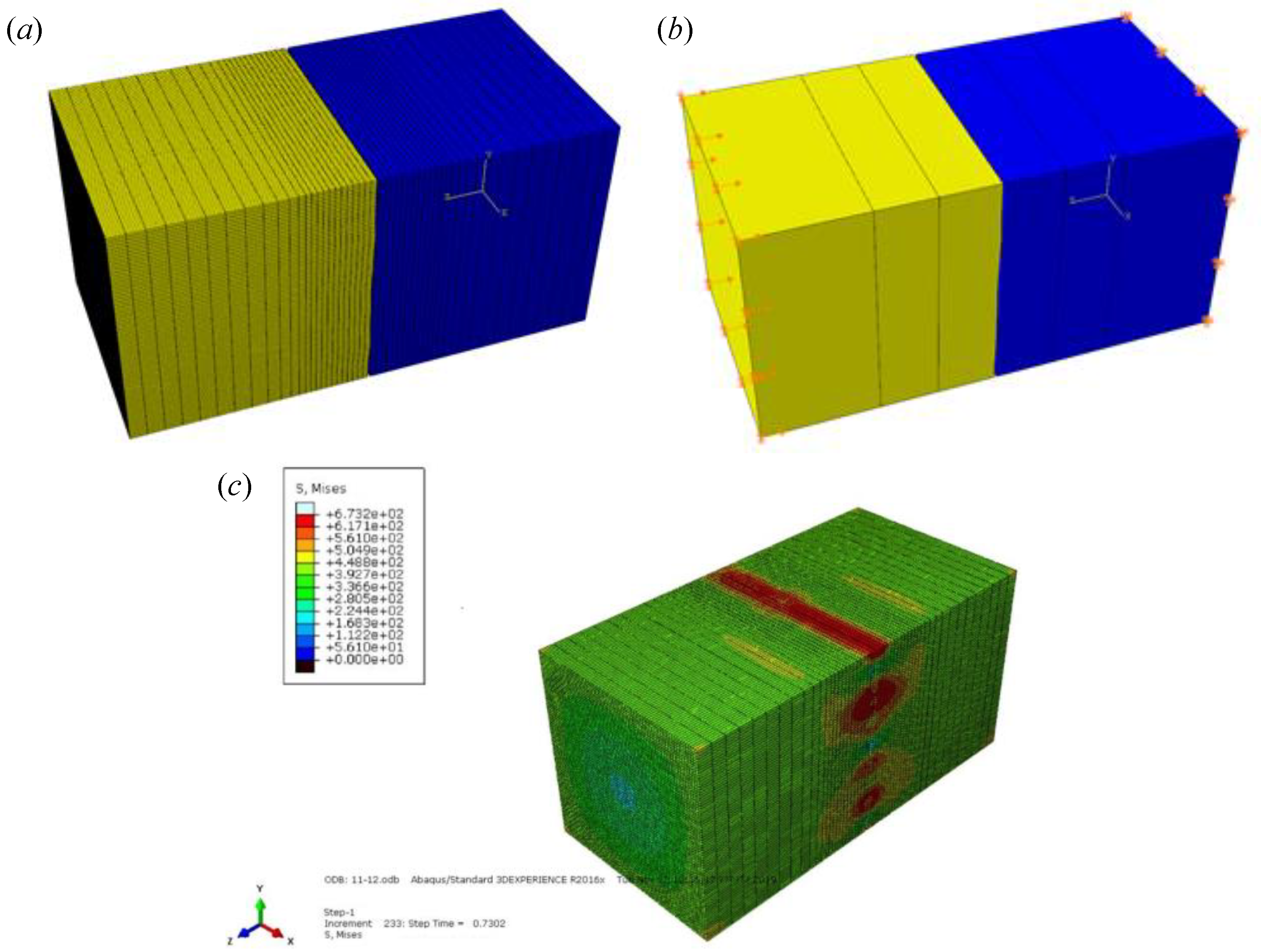
The finite element simulation process includes importing the model, defining contact material properties, assembling the contact model, defining contact types, setting boundary conditions, and outputting the final results. Import the 3D solid model obtained in Section 3.1 into the Abaqus software (6.14, Dassault Systemes S.A, Paris, France). Then, the material properties are defined as follows: elastic modulus E = 210 GPa and Poisson’s ratio ν = 0.3. During the contact process of the rough joint surface, the asperities on the rough surface will participate in the contact firstly. With the increase in contact pressure, the asperities will undergo a transition from elastic deformation to plastic deformation. It should be noted that the contact pressure during plastic deformation of the asperities is far from reaching the yield limit of macro-object deformation. Therefore, combined with the actual contact conditions, it is necessary to define the contact pressure and plastic strain in the plastic deformation. In order to ensure the accuracy of the simulation data, the plastic deformation of the sample is tested by a universal testing machine, and the obtained data are shown in

Table 1. The stress–strain correspondence of plastic deformation.

Stress (MPa)	418	500	605	695	780	829	882	908	921	932	955
Plastic strain (%)	0	1.6	3.0	5.6	9.5	15.8	25.1	35.6	45.5	55.9	65.3

.

After the material properties are defined, the two imported solid models are assembled. Two rough surfaces are set as contact pairs during assembly. In order to avoid interference at the initial position, an initial gap of 30 μm is set between the two rough surfaces. After the assembly is completed, the assembly is meshed. In order to improve the simulation’s efficiency and reduce the software’s running cost, the C3D8R hexahedral grid element is selected as the grid type. In addition, it is worth noting that in order to ensure the accuracy of the simulation results and improve the simulation’s efficiency, during the meshing process, the single 3D model is divided into three regions, and different mesh densities are set in the three regions. The grid sizes set in this paper are 0.001 mm, 0.005 mm, and 0.01 mm. The total number of grids for the two models is 153,260 and 142,852, respectively. The meshing result is shown in Figure 5a.

After meshing, the analysis steps are set as follows: the initial increment step is 1 × 10⁻²⁰, the minimum increment step is 1 × 10⁻²⁰, the maximum increment step is 1 × 10⁻⁵, and the increase in the number of incremental steps is 40,000.

$$k=\frac{\Delta F}{A\cdot \Delta x}$$

(3)

where A is the nominal contact area, ΔF is the variation of contact pressure, and Δx is the variation of contact displacement.

The definition equation of normal contact stiffness is shown in Equation (3). Since the normal contact stiffness cannot be obtained directly from the simulation results, two history outputs of contact pressure and contact displacement need to be created according to Equation (3). In combination with Equation (3), the variation curve of contact stiffness with contact pressure can be obtained. Meanwhile, the field output selects the stress, which is convenient to judge the correctness of the simulation results in the later stage.

After the above process setting is completed, the contact type and boundary conditions need to be set. Set the rough joint surface as face-to-face contact, and the interaction attribute is defined as tangential. The friction formula is set as a penalty function and the friction coefficient is set as 0.15 [34]. The load application results are shown in Figure 5b. The boundary condition is set as the load form with one end fixed and one end set with displacement. The displacement is set at four times the turning residual height R_t.

After the above process settings are completed, the simulation results can be obtained by submitting the job. The stress cloud diagram of the simulation results is shown in Figure 5c.

4. Comparison and Analysis of Results

In order to verify the accuracy of the finite element results in this paper, the finite element results, the analytical results of the KE model, and the experimental results are compared and analyzed. Then, the finite element simulation results under different machining parameters are compared, and the influence of machining parameters on the normal contact stiffness is explored.

4.1. Comparison Results under Different Methods

In order to ensure the comparability of different results, the work-piece is first processed by the combined machining mode. Meanwhile, the processing parameters are recorded, which is convenient for modeling the surface topography under the combined processing mode. In addition, the ZYGONexView non-contact micro-topography measurement system (ZYGO Corporation, Middlefield, CT, USA) is used to measure the micro-surface topography of the work-piece, which is convenient to obtain the initial value for the analytical calculation of the KE model. The analytical calculation process of the KE model is carried out according to the literature [16]. Due to space limitations, the specific process will not be repeated here. After the measurement of the surface topography, the experimental test can be carried out, and the experimental process is carried out according to the literature [11]. A schematic diagram and physical drawings of the contact stiffness test rig are shown in Figure S2. The experimental process is described in detail in the supplementary material. After processing the experimental data, the experimental results for the normal contact stiffness can be obtained. Furthermore, in order to ensure the reliability of the comparison results, each result is calculated three times respectively, and the average value of the three results is taken as the final result for display.

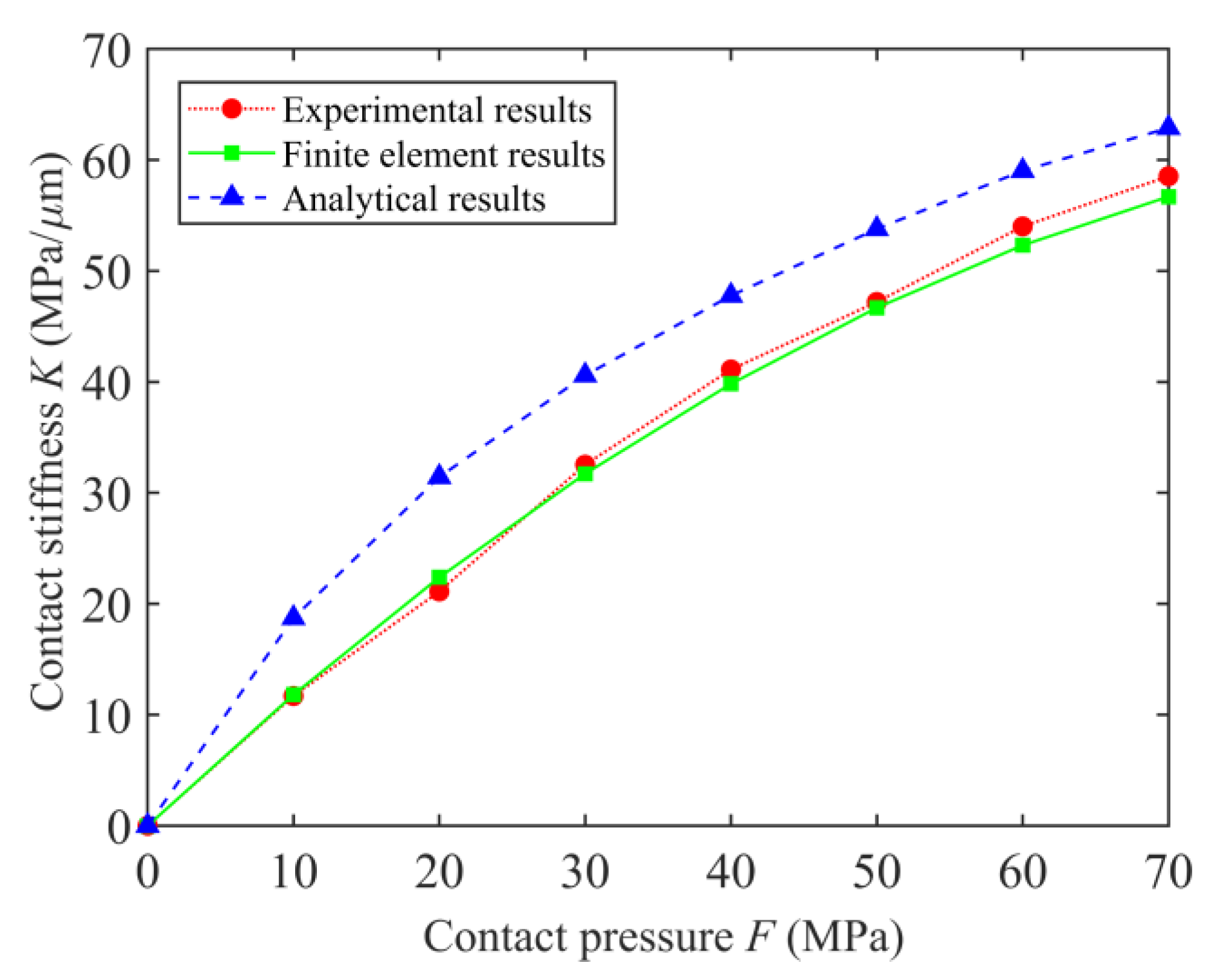
The finite element results, the analytical results of the KE model, and the experimental results are compared and analyzed firstly. The initial machining parameters are r = 0.2 mm, f = 0.2 mm/r, D = 2.5, G = 1 × 10⁻⁸, and δ_d = 80% respectively. The comparison results of normal contact stiffness under different methods are shown in Figure 6.

Based on the comparison results in Figure 6, the finite element results and the analytical results of the KE model have the same change trend as the experimental results. The comparison values of the contact stiffness and the relative error can be found in Table S1. The normal contact stiffness increases with the increase in contact pressure. When the contact pressure F = 70 MPa, the contact stiffness reaches the maximum values, which are 56.69 MPa/μm, 57.54 MPa/μm, and 62.89 MPa/μm, respectively. However, under the same contact pressure, there are differences among the three results, and this difference changes with the change in contact pressure. It can be seen from Figure 6 that under the same contact pressure, the analytical results of the KE model have larger values than other results. What is exciting is that the finite element results in this paper differ slightly from the experimental results. Segmental analysis of the results was performed. When F < 30 MPa, the difference between the three results gradually increased. However, with the further increase in the contact pressure, the difference between the three showed a decreasing trend. The maximum relative error between the finite element results and the experimental results is 6.03%, while the maximum relative error between the analytical results of the the KE model and experimental results is 60.07%.

The above results are analyzed in combination with the distribution and deformation laws of asperities on the rough surface. Firstly, with the continuous increase in the contact pressure, the number of asperities involved in the contact on the rough surface increases, resulting in a gradual increase in the contact stiffness. Secondly, when the contact pressure is small, the asperities that actually participate in the contact are formed by grinding. For the KE model, the model adopts the assumption of asperities with a uniform shape. The size of the asperities is obtained by averaging, and the contact process does not involve changes in the types of asperities. More importantly, in the process of calculating the asperity parameters, the turning topography that does not participate in the contact is included. The above reasons lead to an increase in the number of asperities involved in the contact during the analytical calculation process, which in turn causes the analytical results obtained at the initial stage of contact to be much larger than the real working conditions. With the increase in the contact pressure, the number of asperities participating in the contact increases. The difference between the analytical results and the other results will also gradually decrease. Finally, under the same contact pressure, the finite element results are slightly smaller than the experimental results, and the relative error between them is small. This phenomenon can also be attributed to asperities on the rough surface. In the process of surface modeling, some approximations are made for the surface topography. The built model fails to fully reflect all the details of the actual surface, resulting in the finite element results being slightly smaller than the experimental results.

4.2. Comparison Results under Different Machining Parameters

The following is the comparative analysis of the finite element results under different machining parameters. The machining parameters include the arc radius of the turning tools, the turning feed rate, the grinding depth, the fractal dimension, and the scale coefficient. The comparison values of the contact stiffness can be found in Tables S2–S6.

4.2.1. Turning Tool Arc Radius

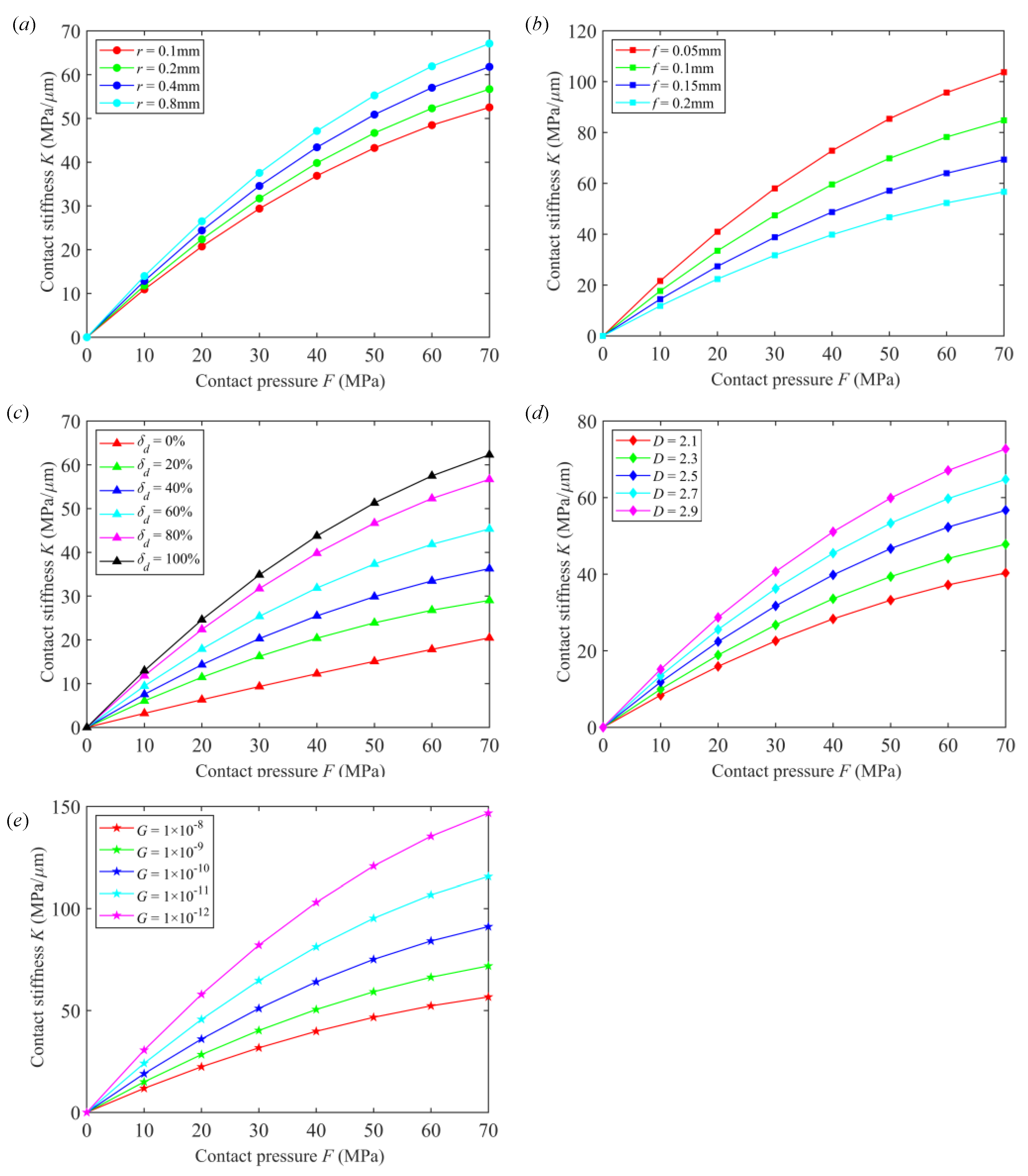
Figure 7a shows the comparison results for the contact stiffness under different turning tool arc radii. The arc radii of the turning tool are 0.1 mm, 0.2 mm, 0.4 mm, and 0.8 mm, respectively, and the other machining parameters are f = 0.2 mm/r, D = 2.5, G = 1 × 10⁻⁸, and δ_d = 80%, respectively.

Based on the comparison results in Figure 7a, under the condition of the turning tool having the same arc radius, the normal contact stiffness increases with the increase in the contact pressure. When the contact pressure F = 70 MPa, the contact stiffness reaches the maximum values, which are 52.53 MPa/μm, 56.69 MPa/μm, 61.80 MPa/μm, and 67.11 MPa/μm, respectively. The above results can be analyzed in combination with the distribution and deformation laws of asperities on the rough surface. Under the condition of the same arc radius and with the continuous increase in the contact pressure, the number of asperities involved in the contact on the rough surface increases, resulting in a gradual increase in the contact stiffness.

Meanwhile, under the same contact pressure, the contact stiffness increases gradually with the increase in the arc radius. Under the condition of the same contact pressure, there are differences in the asperities involved in the contact under the conditions of different arc radii. Combined with Equation (1), with the increase in the arc radius, the residual height R_t of the turning surface decreases gradually. The decrease in R_t will increase the stability of the rough interface, which in turn leads to an increase in the normal contact stiffness.

4.2.2. Turning Feed Rate

Figure 7b shows the comparison results for contact stiffness under different turning feed rates. The turning feed rates are 0.05 mm/r, 0.1 mm/r, 0.15 mm/r, and 0.2 mm/r, respectively. Other parameters are r = 0.2 mm, D = 2.5, G = 1 × 10⁻⁸, and δ_d = 80%, respectively.

Based on the comparison results in Figure 7b, under the condition of the same turning feed rate, the normal contact stiffness increases with the increase in the contact pressure. When the contact pressure F = 70 MPa, the contact stiffness reaches the maximum values, which are 56.69 MPa/μm, 69.34 MPa/μm, 84.80 MPa/μm, and 103.71 MPa/μm, respectively. The above results can be analyzed in combination with the distribution and deformation laws of asperities on the rough surface. Under the same turning feed rate and with the continuous increase in the contact pressure, the number of asperities involved in the contact on the rough surface increases, resulting in an increase in the contact stiffness.

Meanwhile, under the same contact pressure, the contact stiffness decreases gradually with the increase in the turning feed rate. Under the same contact pressure, there are differences in the asperities involved in the contact under different turning feed rates. Combined with Equation (1), with the increase in the turning feed rate, the residual height R_t of the turning surface decreases gradually. The decrease of R_t will increase the stability of the rough joint surface, which in turn leads to an increase in the normal contact stiffness.

Moreover, for different contact pressures, the difference in contact stiffness under different feed rates is different, and this difference increases gradually with the increase in contact pressure. The difference in contact stiffness under different contact pressures is explained as follows. When the contact pressure is small, the asperities that actually participate in the contact are formed by grinding. Since the model surface is basically identical to the actual surface, the results for the normal contact stiffness will be almost the same. However, with the increase in contact pressure, the asperities produced by turning will occupy a dominant position. With the increase in the turning feed rate, the residual height of the asperities on the turning surface increases, and the density of the asperities on the turning surface per unit area decreases. In turn, the difference in normal contact stiffness increases gradually with the increase in contact pressure.

4.2.3. Grinding Depth

Figure 7c shows the comparison results for contact stiffness under different grinding depths. The grinding depth is taken as 0%, 20%, 40%, 60%, 80%, and 100% of the turning residual height, respectively. Other machining parameters are r = 0.2 mm, f = 0.2 mm/r, D = 2.5 and, G = 1 × 10⁻⁸, respectively.

Based on the comparison results in Figure 7c, under the condition of the same grinding depth, the normal contact stiffness increases with the increase in the contact pressure. When the contact pressure F = 70 MPa, the contact stiffness reaches the maximum values, which are 20.47 MPa/μm, 29.03 MPa/μm, 36.28 MPa/μm, 45.35 MPa/μm, 56.69 MPa/μm, and 62.30 MPa/μm, respectively. The above results can be analyzed in combination with the distribution and deformation laws of asperities on the rough surface. Under the condition of the same arc radius and with the continuous increase in the contact pressure, the number of asperities involved in the contact on the rough surface increases, resulting in a gradual increase in the contact stiffness.

Meanwhile, under the same contact pressure, the contact stiffness increases gradually with the increase in the grinding depth. Under the condition of the same contact pressure, there are differences in the asperities involved in the contact under the condition of different grinding depths. With the increase in the grinding depth, the proportion of the grinding surface in the combined machining surface increases gradually. Combined with the asperities on the rough surface, as the grinding depth increases, the size of the asperities on the rough surface is smaller, and the distribution density of the asperities is greater. The above factors will cause the normal contact stiffness to increase gradually with the increase in grinding depth.

4.2.4. Fractal Dimension

Figure 7d shows the comparison results for contact stiffness under different fractal dimensions. The fractal dimensions are 2.1, 2.3, 2.5, 2.7, and 2.9, respectively. Other machining parameters are r = 0.2 mm, f = 0.2 mm/r, G = 1 × 10⁻⁸, and δ_d = 80%, respectively.

Based on the comparison results in Figure 7d, under the condition of the same fractal dimension, the normal contact stiffness increases with the increase in the contact pressure. When the contact pressure F = 70 MPa, the contact stiffness reaches the maximum values, which are 40.33 MPa/μm, 47.82 MPa/μm, 56.69 MPa/μm, 64.76 MPa/μm, and72.73 MPa/μm, respectively. The above results can be analyzed in combination with the distribution and deformation laws of asperities on the rough surface. Under the condition of the same fractal dimension and with the continuous increase in the contact pressure, the number of asperities involved in the contact on the rough surface increases, resulting in a gradual increase in the contact stiffness.

Meanwhile, under the same contact pressure, the contact stiffness increases gradually with the increase in the grinding depth. Under the condition of the same contact pressure, there are differences in the asperities involved in the contact under the conditions of different fractal dimensions. With the increase in the fractal dimension, the density and number of asperities on the rough surface increase. The above factors will cause the normal contact stiffness to increase gradually with the increase in the fractal dimension.

4.2.5. Scale Coefficient

Figure 7e shows the comparison results for contact stiffness under different scale coefficients. The scale coefficients are 10⁻⁸, 10⁻⁹, 10⁻¹⁰, 10⁻¹¹, and 10⁻¹², respectively. Other parameters are r = 0.2 mm, f = 0.2 mm/r, D = 2.5, and δ_d = 80%, respectively.

Based on the comparison results in Figure 7e, under the condition of the same scale coefficient, the normal contact stiffness increases with the increase in the contact pressure. When the contact pressure F = 70 MPa, the contact stiffness reaches the maximum values, which are 56.69 MPa/μm, 71.91 MPa/μm, 91.21 MPa/μm, 115.69 MPa/μm, and 146.74 MPa/μm, respectively. The above results can be analyzed in combination with the distribution and deformation laws of asperities on the rough surface. Under the condition of the same scale coefficient, with the continuous increase in the contact pressure, the number of asperities involved in the contact on the rough surface increases, resulting in a gradual increase in the contact stiffness.

Meanwhile, under the same contact pressure, the contact stiffness decreases gradually with the increase in the scale coefficient. Under the condition of the same contact pressure, there are differences in the asperities involved in the contact under the conditions of different scale coefficients. With the increase in the scale factor, the contour amplitude of the asperities on the rough surface increases. The increase in the profile amplitude will lead to a decrease in the stability of the joint surface, which will cause the normal contact stiffness to gradually decrease with the increase in the scale coefficient.

5. Conclusions

The normal contact stiffness of the joint surface machined by turning and grinding is studied by the finite element method. The comparison results show that the finite element results are more accurate than the analytical results of the KE model. In addition, the finite element calculation results of normal contact stiffness under different machining parameters are compared. The normal contact stiffness increases with the increase in the turning tool arc radius, the grinding depth, and the fractal dimension, and decreases with the increase in the feed rate and the proportional coefficient. The method proposed in this paper provides a novel method for accurately obtaining the normal contact stiffness of rough joint surfaces under a combined machining mode and has guiding significance for machining production.

However, the modeling process fails to fully reflect the full details of the actual topography, which leads to deviations between the finite element results and the experimental results. How to improve the modeling accuracy will be carried out in future work.

References

- Zhou, H.; Long, X.H.; Meng, G.; Liu, X.B. A stiffness model for bolted joints considering asperity interactions of rough surface contact. J. Tribol. Trans. Asme 2022, 144, 011501. [Google Scholar] [CrossRef]
- Liu, Y.; Suo, S.; Meng, G.; Li, D. Study on the resonance restraint of a large hoist system headframe. Int. J. Struct. Stab. Dyn. 2020, 20, 2050109. [Google Scholar] [CrossRef]
- Zhang, K.; Li, G.; Gong, J.Z.; Zhang, M. Normal contact stiffness of rough surfaces considering oblique asperity contact. Adv. Mech. Eng. 2019, 11, 1–14. [Google Scholar] [CrossRef] [Green Version]
- Yu, X.; Sun, Y.Y.; Zhao, D.; Wu, S.J. A revised contact stiffness model of rough curved surfaces based on the length scale. Tribol. Int. 2021, 164, 107206. [Google Scholar] [CrossRef]
- Li, L.; Wang, J.J.; Shi, X.H.; Ma, S.L.; Cai, A.J. Contact stiffness model of joint surface considering continuous smooth characteristics and asperity interaction. TriL 2021, 69, 43. [Google Scholar] [CrossRef]
- Ghaednia, H.; Wang, X.; Saha, S.; Xu, Y.; Sharma, A.; Jackson, R. A review of elastic-plastic contact mechanics. ApMRv 2018, 69, 060804. [Google Scholar] [CrossRef] [Green Version]
- Greenwood, J.A.; Williamson, J.B.P. Contact of nominally flat surfaces. Proc. R. Soc. A Math. Phys. Eng. Sci. 1966, 295, 300–319. [Google Scholar] [CrossRef]
- Bush, A.W.; Gibson, R.D.; Thomas, T.R. The elastic contact of a rough surface. Wear 1975, 35, 87–111. [Google Scholar] [CrossRef]
- Komvopoulos, K.; Choi, D.H. Elastic finite element analysis of multi-asperity contacts. J. Tribol. 1992, 114, 823–831. [Google Scholar] [CrossRef]
- Horng, J.H. An elliptic elastic-plastic asperity microcontact model for rough surfaces. J. Tribol. 1998, 120, 82–88. [Google Scholar] [CrossRef]
- An, Q.; Suo, S.F.; Lin, F.Y.; Shi, J.W. A novel micro-contact stiffness model for the grinding surfaces of steel materials based on cosine curve-shaped asperities. Materials 2019, 12, 3561. [Google Scholar] [CrossRef] [PubMed] [Green Version]
- Chang, W.R.; Etsion, I.; Bogy, D.B. An elastic-plastic model for the contact of rough surfaces. J. Tribol. 1987, 109, 257–263. [Google Scholar] [CrossRef]
- Zhao, Y.; Maietta, D.M.; Chang, L. An asperity microcontact model incorporating the transition from elastic deformation to fully plastic flow. J. Tribol. 2000, 122, 86–93. [Google Scholar] [CrossRef]
- Zhao, Y.; Chang, L. A model of asperity interactions in elastic-plastic contact of rough surfaces. J. Tribol. 2001, 123, 857–864. [Google Scholar] [CrossRef]
- Ciavarella, M.; Greenwood, J.A.; Paggi, M. Inclusion of “interaction” in the Greenwood and Williamson contact theory. Wear 2008, 265, 729–734. [Google Scholar] [CrossRef]
- Kogut, L.; Etsion, I. A finite element based elastic-plastic model for the contact of rough surfaces. Tribol. Trans. 2003, 46, 383–390. [Google Scholar] [CrossRef]
- Chandrasekar, S.; Eriten, M.; Polycarpou, A.A. An improved model of asperity interaction in normal contact of rough surfaces. J. Appl. Mech. 2013, 80, 011025. [Google Scholar] [CrossRef]
- Ciavarella, M. Rough contacts near full contact with a very simple asperity model. Tribol. Int. 2016, 93, 464–469. [Google Scholar] [CrossRef]
- Gao, Z.; Fu, W.; Wen, W.; Kang, W.; Liu, Y. The study of anisotropic rough surfaces contact considering lateral contact and interaction between asperities. Tribol. Int. 2018, 126, 270–282. [Google Scholar] [CrossRef]
- Du, F.; Hong, J.; Xu, Y. An acoustic model for stiffness measurement of tribological interface using ultrasound. Tribol. Int. 2014, 73, 70–77. [Google Scholar] [CrossRef]
- Mulvihill, D.M.; Brunskill, H.; Kartal, M.E.; Dwyer-Joyce, R.S.; Nowell, D. A comparison of contact stiffness measurements obtained by the digital Image correlation and ultrasound techniques. ExM 2013, 53, 1245–1263. [Google Scholar] [CrossRef] [Green Version]
- Yazman, Ş.; Gemı, L.; Uludağ, M.; Akdemır, A.; Uyaner, M.; Dişpinar, D. Correlation Between Machinability and Chip Morphology of Austempered Ductile Iron. J. Test. Eval. 2018, 46, 20160490. [Google Scholar] [CrossRef]
- Yazman, Ş.; Köklü, U.; Urtekin, L.; Morkavuk, S.; Gemi, L. Experimental study on the effects of cold chamber die casting parameters on high-speed drilling machinability of casted AZ91 alloy. J. Manuf. Processes 2020, 57, 136–152. [Google Scholar] [CrossRef]
- Yazman, Ş. The effects of back-up on drilling machinability of filament wound GFRP composite pipes: Mechanical characterization and drilling tests. J. Manuf. Processes 2021, 68, 1535–1552. [Google Scholar] [CrossRef]
- Uludağ, M.; Yazman, Ş.; Gemi, L.; Bakircioğlu, B.; Erzi, E.; Dispinar, D. Relationship Between Machinability, Microstructure, and Mechanical Properties of Al-7Si Alloy. J. Test. Eval. 2018, 46. [Google Scholar] [CrossRef]
- Aamir, M.; Davis, A.; Keeble, W.; Koklu, U.; Giasin, K.; Vafadar, A.; Tolouei-Rad, M. The Effect of TiN-, TiCN-, TiAlN-, and TiSiN Coated Tools on the Surface Defects and Geometric Tolerances of Holes in Multi-Spindle Drilling of Al2024 Alloy. Metals 2021, 11, 1103. [Google Scholar] [CrossRef]
- Lee, W.B.; Cheung, C.F. A dynamic surface topography model for the prediction of nano-surface generation in ultra-precision machining. Int. J. Mech. Sci. 2001, 43, 961–991. [Google Scholar] [CrossRef]
- Qi, A.; Suo, S.; Yan, L.; Li, Y.; Shi, J. Feature decoupling and shape simulation of turning rough surface. J. Mech. Eng. 2019, 55, 200–209. [Google Scholar] [CrossRef]
- Chen, B.; Luo, L.; Jiao, H.; Li, S.; Deng, Z.; Yao, H. Affecting factors, optimization, and suppression of grinding marks: A review. Int. J. Adv. Manuf. Technol. 2021, 115, 1–29. [Google Scholar] [CrossRef]
- Chen, C.; Tang, J.; Chen, H.; Zhu, C. Research about modeling of grinding workpiece surface topography based on real topography of grinding wheel. Int. J. Adv. Manuf. Technol. 2017, 93, 2411–2421. [Google Scholar] [CrossRef]
- Yan, W.; Komvopoulos, K. Contact analysis of elastic-plastic fractal surfaces. J. Appl. Phys. 1998, 84, 3617–3624. [Google Scholar] [CrossRef]
- Yu, Z.Q.; Wang, T.Y.; Wang, P.; Tian, Y.; Li, H.B. Rapid and precise reverse engineering of complex geometry through multi-sensor data fusion. IEEE Access 2019, 7, 165793–165813. [Google Scholar] [CrossRef]
- Huang, W.H.; Jiang, Z.G.; Wang, T.; Wang, Y.; Hu, X.L. Remanufacturing scheme design for used parts based on incomplete information reconstruction. Chin. J. Mech. Eng. 2020, 33, 1–14. [Google Scholar] [CrossRef]
- Shi, W.B.; Zhang, Z.S. Contact characteristic parameters modeling for the assembled structure with bolted joints. Tribol. Int. 2022, 165, 107272. [Google Scholar] [CrossRef]
Figure 1.
Turning mode. (a) The schematic diagram of the modeling principle; (b) 3D turning topography under r = 0.2 mm and f = 0.2 mm/r.
Figure 2.
3D fractal surface. (a) Modeling process; (b) 3D fractal surface under D = 2.5 and G = 1 × 10⁻⁸.
Figure 3.
Surface topography under the combined machining mode. (a) The schematic diagram of the 2D topography; (b) The schematic diagram of the 3D topography.
Figure 4.
Reverse modeling results. (a) Point cloud data; (b) Mesh file; (c) Feature surface; (d) Solid mode.
Figure 5.
Finite element processing flow. (a) Meshing result; (b) Load application and boundary conditions; (c) Stress cloud diagram of the simulation result.
Figure 6.
Comparison results of normal contact stiffness under different methods.
Figure 7.
Comparison results for normal contact stiffness. (a) Different arc radii of turning tools; (b) Different turning feed rates; (c) Different grinding depths; (d) Different fractal dimensions; (e) Different scale coefficients.