
Prediction of Fracture Toughness Scatter Based on Weibull Stress Using Crystal Plasticity Finite Element Method


1
College of Mechanical Engineering, Zhejiang University of Technology, Hangzhou 310032, China
2
Shanghai Nuclear Engineering Research & Design Institute Co., Ltd., Shanghai 200233, China
3
Engineering Research Center of Process Equipment and Re-Manufacturing, Ministry of Education, Hangzhou 310032, China
*
Author to whom correspondence should be addressed.
Metals 2022, 12(5), 872; https://0-doi-org.brum.beds.ac.uk/10.3390/met12050872
Submission received: 1 March 2022
/
Revised: 17 May 2022
/
Accepted: 18 May 2022
/
Published: 20 May 2022
Abstract
:A multi-scale prediction method was proposed to investigate the scatter of fracture toughness by combining the local approach (LA) to cleavage fracture and the crystal plasticity finite element method (CPFEM). The parameters in the crystal plasticity constitutive model were firstly determined by comparing the simulated stress-strain curves with tested curves for SA508-III steel. Then CT samples were modeled using the CPFEM to calculate Weibull stress. Using the calibration process of local approach, the relevant parameters of the Beremin model were obtained with m = 30 and σu = 2590 MPa. The fracture toughness was analyzed including the scatter for a given temperature, the master curve in a temperature range. The distribution of predicted fracture toughness shows good agreement with the test results. All of the tested fracture toughness value are fall in the range of 5% to 95% that precited using the proposed combined approach.
1. Introduction
In nuclear power plants, reactor pressure vessels (RPVs) play an important significant role in protecting reservation of reactor safety. It is necessary to be ensured the structural integrity of RPVs for the safe operation of nuclear power plants. A major input parameter for assessing the structural integrity of the RPV is the fracture toughness of ferritic steels generally adopted for RPVs, which present significant scatter in the ductile-to-brittle transition (DTB) region [1]. In addition, neutron irradiation during RPV operation will produce an embrittlement effect, inducing the reduction of fracture toughness, which may be related to the microstructure evolution of RPV steel, referring to the change of pores and grain orientation [2,3,4,5]. The microstructure change will affect the fracture toughness of materials, so it is very important to study the fracture toughness from the microscopic point of view.
The theory of crystal plasticity with the consideration of microstructure has been applied and researched in the study of fracture behavior of metals, which can be traced back to Taylor’s crystal plasticity dislocation motion theory in 1938 [6]. Subsequently, Hill, Rice, Peirce, and many other scholars continued to study and modify the crystal plasticity theory with Voronoi technology combined, widely introducing the crystal plasticity theory in various fields [7,8,9].
Wan [10] studied the fracture mechanism of SA508-III steel and found that the decrease in fracture toughness is caused by material hardening, and indicated that dislocation ring voids inside the material will affect dislocation slip. Li and Zhou [11,12] established a microscopic finite element model by correlating the microstructure with the fracture toughness of materials to analyze the effect of microstructure changes on fracture toughness, and showed that the fine microstructure size can effectively elevate the material’s fracture toughness. Vincent [13] proposed a new crystal plasticity model to discuss the effect of temperature and irradiation hardening on fracture toughness based on the stress heterogeneity. Liu [14] simulated the three-point bending test process through crystal plastic finite element. They studied the fracture toughness of SA508-III steel at different temperatures in combination with the Beremin local approach. Chen [15] proposed a constitutive probability model of fracture toughness associated with temperature depending on crystal plasticity theory and explored the cleavage and competition between pores of ferrite or martensite at different temperatures. Roy [16] studied the effect of microstructure orientation on the fracture behavior of polycrystalline metal, and established a prediction method of the fracture toughness of metal based on the microstructure properties.
For the scatter of fracture toughness, a commonly used method is the Beremin cleavage fracture local approach (LA) [17], where the cleavage fracture of materials is predicted from a micromechanics perspective using a Weibull distribution. Mathieu [18] took 16MND5 as the model material to study the application of the Beremin local approach in the brittle fracture of low alloy steel. Qian [19,20] used two finite element models, namely ideal elastic-plastic model and actual elastic-plastic model, to study the influence of temperature on model parameters in the local method of induced fracture. The results showed the model parameters were independent of temperature. Cao [21] investigated the fracture toughness of 16MnDR by the master curve approach, as well as the effect of temperature on Beremin model parameters, and the temperature dependency of critical parameters. Chang [22] explored the relationship of Beremin parameters with temperature, loading speed, and constraint, reporting that the related parameters can be considered material constants independent from temperature, acceleration, and constraint.
In summary, the crystal plasticity finite element method and the local approach have been widely applied to studies on material fracture toughness. However, it is necessary to explain the effect of crystallographic feature on the fracture toughness, especially for the temperature dependency and the randomness. The combination of CPFEM and LA is proposed to investigate these effects for the typical RPV steel SA508-III.
The paper is organized as follows. In Section 2, the crystal plasticity constitutive model and the slip system of SA508-III steel are described. In Section 3, a 2D crystal plasticity finite element model is established based on crystal plasticity theory. In addition, the tensile test is simulated to determine the material parameters at different temperatures. Then compact tensile samples of different sizes are analyzed using the material parameters that calibrated crystal plasticity model. In Section 4, fracture toughness experiments are carried out from −100 °C to 20 °C. The Beremin local approach is introduced to describe the scatter of fracture toughness values. In Section 5, the model parameters of the local approach are calibrated on the test results using the stress field obtained by the CPFEM. The randomness and the temperature dependency are discussed on the predicted fracture toughness. In Section 6, some conclusions are drawn.
2. Crystal Plasticity Theory
2.1. Crystal Plastic Constitutive Model
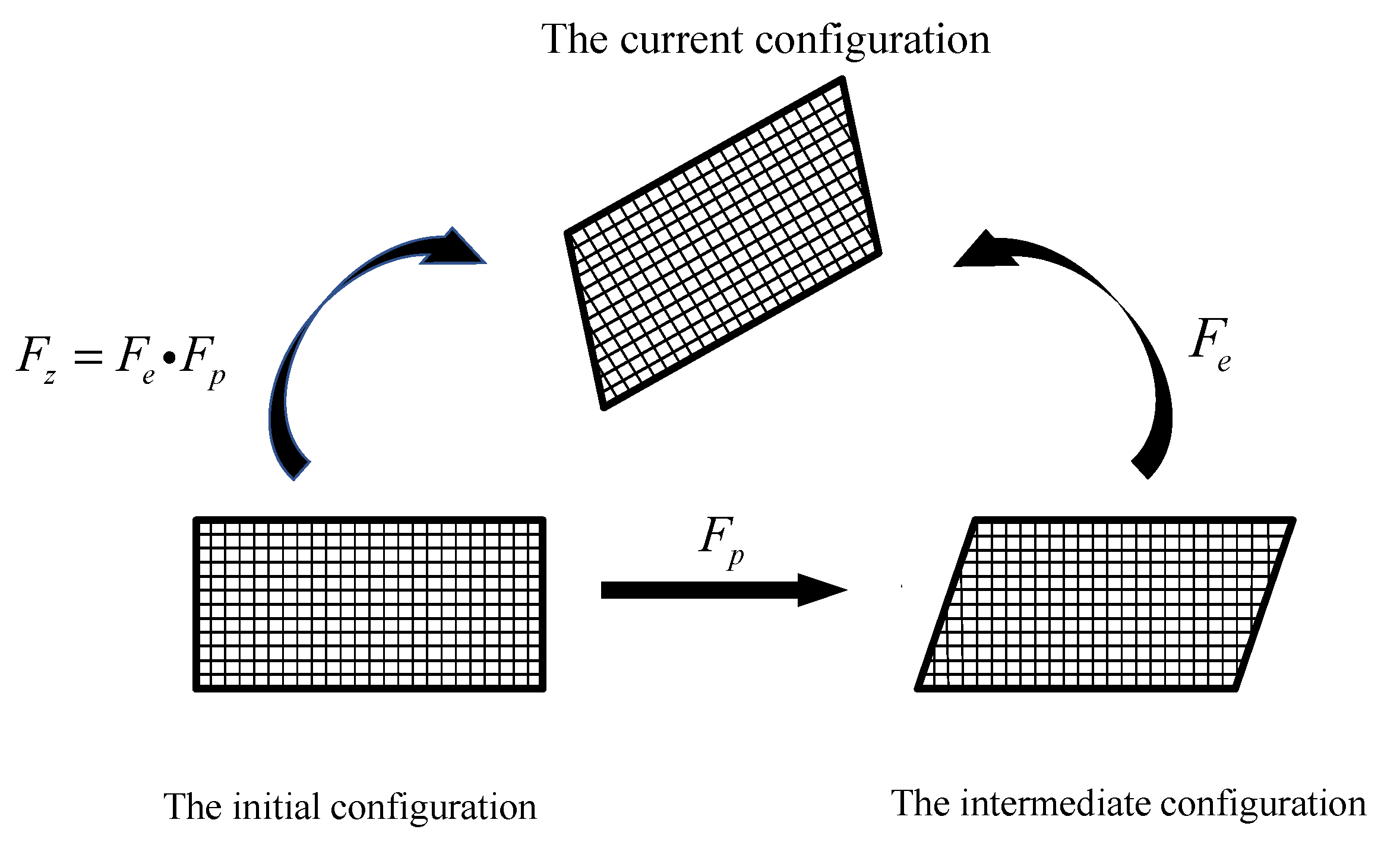
In this research, the elastic plastic finite deformation analysis theory of Hill and Rice [7] is used to explore the deformation behavior of SA508-III steel. The crystal deformation under external force can be decomposed into elastic deformation and plastic deformation. Then crystal deformation gradient F can be decomposed as [23]:
where is the elastic deformation gradient generated during crystal deformation, is the plastic deformation gradient corresponding to uniform shear of crystal along the slip direction. Therefore, through the influence of the above two deformation gradients, the deformation of grains can be divided into three configurations: initial configuration, intermediate configuration and current configuration. First, the material moves from the initial configuration to the intermediate configuration through the deformation gradient . This process only produces plastic shear deformation and crystal slip. Then the intermediate configuration moves to the current configuration through the deformation gradient , and lattice distortion and rotation occur in this process. The grain deformation process is shown in Figure 1 [7].
Similar to the deformation gradient, the velocity gradient can also be decomposed into two parts corresponding to slip and lattice distortion plus rigid body rotation:
where, L is the velocity gradient, is the velocity gradient caused by elastic deformation, and is the velocity gradient caused by plastic deformation, which can be determined by the sum of shear strain rates in all slip systems, following [7]:
where, is the dislocation slip rate of the α slip system, is the unit vector of the slip direction in the α slip system, is the unit normal vector of the slip surface on the α slip system, and N is the total number of slip systems. is the Schmid tensor.
The dislocation slip rate is the key to the realization of the crystal plastic constitutive model. The relationship between the dislocation slip rate and the shear stress can be obtained through the hardening Equation [8].
where, is the reference dislocation slip rate. is the critical resolved shear stress of slip system α. is a material constant for all slip systems when . n is a rate sensitive parameter of slip system α. The model reverts to a rate-independent plastic state with a large value of n, and the material tends to be viscoelastic for n = 1. The shear stress , also known as Schmid stress.
In general, the reference shear stress increases with the deformation and reference shear stress rate can be characterized by the hardness of the slip system [8], as follows:
where, is the n × n hardening coefficient matrix, an instantaneous value that changes continuously during the deformation process. The hardening coefficient can be determined according to Peirce [8] as follows:
where, is Kronecker matrix, if α = β, = 1, otherwise = 0. is a self-hardening coefficient, which indicates the change rate of critical shear stress with shear strain. ratio of latent hardening rates to self-hardening rates was assumed to be 1.0, which will be degenerated to the original work by Taylor [6]. Asaro [24] used the corresponding formula for the self-hardening coefficient:
where, is the initial hardening rate, is the deformation resistance of the slip system at the initial yield of the material (the initial flow stress), is the saturation value of the deformation resistance of the slip system (the saturated flow stress). All of the three parameters are material constants.
2.2. Determination of Crystal Slip System
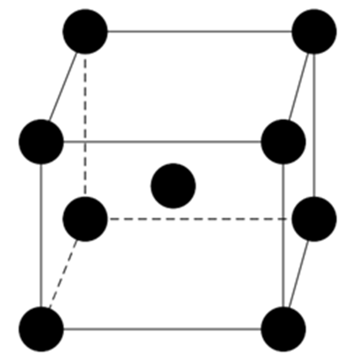
The slip systems vary with different crystal types. The main research object of this paper is SA508-III steel, which is ferritic steel with a body-centered cubic (bcc) structure, as shown in Figure 2. A bcc crystal has three slip planes, {110}, {112} and {123}, with the initial slip direction of <111>. The slip usually occurs on the slip planes {110} and {112}, so the slip systems located on {110} or {112} slip planes are defined as potential slip systems. The slip plane will change with the influence of temperature, which is generally {112} at low temperature and {110} at medium temperature [25]. Therefore, this work focused on the two slip systems, {110} <111> and {112} <111>, as listed in Table 1 and Table 2.
3. Determination of Model Parameters
3.1. Voronoi Model
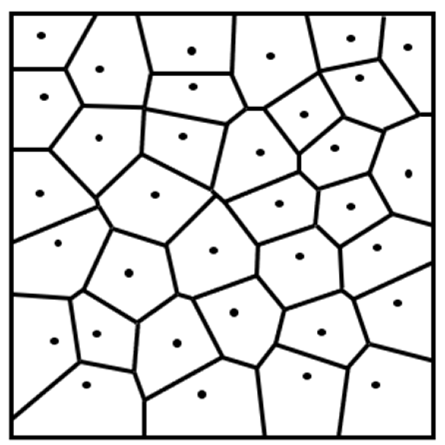
Most of the metals are polycrystalline materials with metal grains of various sizes and shapes, where the grain orientations of some polycrystalline materials have a certain orientation tendency, while others belong to random orientations [25]. To simulate the grains, the Voronoi method is adopted to construct the polycrystalline model, which was proposed by Voronoi [9]. A typical 2D Voronoi is shown in Figure 3.
3.2. Tension Simulation
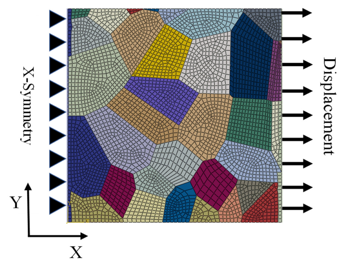
Firstly, the uniaxial tensile test is simulated using a 2D plane model. Compared with the test results, the material parameters in the crystal plastic constitutive model can be determined depending on the trials with tension simulations [26]. According to Zhang [25] and He [27], the grain size of SA508-III steel is about 20~30 μm. A 2D Voronoi tensile model was established as shown in Figure 3. The Voronoi model of the stretch simulation with boundary conditions and mesh is depicted in Figure 4. A local square model with 0.15 × 0.15 mm2 is adopted containing 35 grains with random orientation. The tensile test was conducted according to American Society of Testing Materials E8/E8M-16ae1 [28], (ASTM E8/E8M-16ae1) [28], with the strain rate of 4 × 10⁻⁴/s, and the maximum displacement deformation of 20% of the overall size. The simulation was run in the ABAQUS finite element software (Le Groupe Dassault, Vaucresson, France), applying the UMAT subroutine designed by Huang [29].
The UMAT subroutine requires material parameters as described in Section 2, include three independent elastic constants C11, C12, and C44 that define the elastic stiffness matrix, and material constants that describe the rate-dependent hardening criterion: , , , h0, n. Referencing Liu and Raabe’s simulation process [14,30], these material parameters at different temperatures are determined through trial and error.
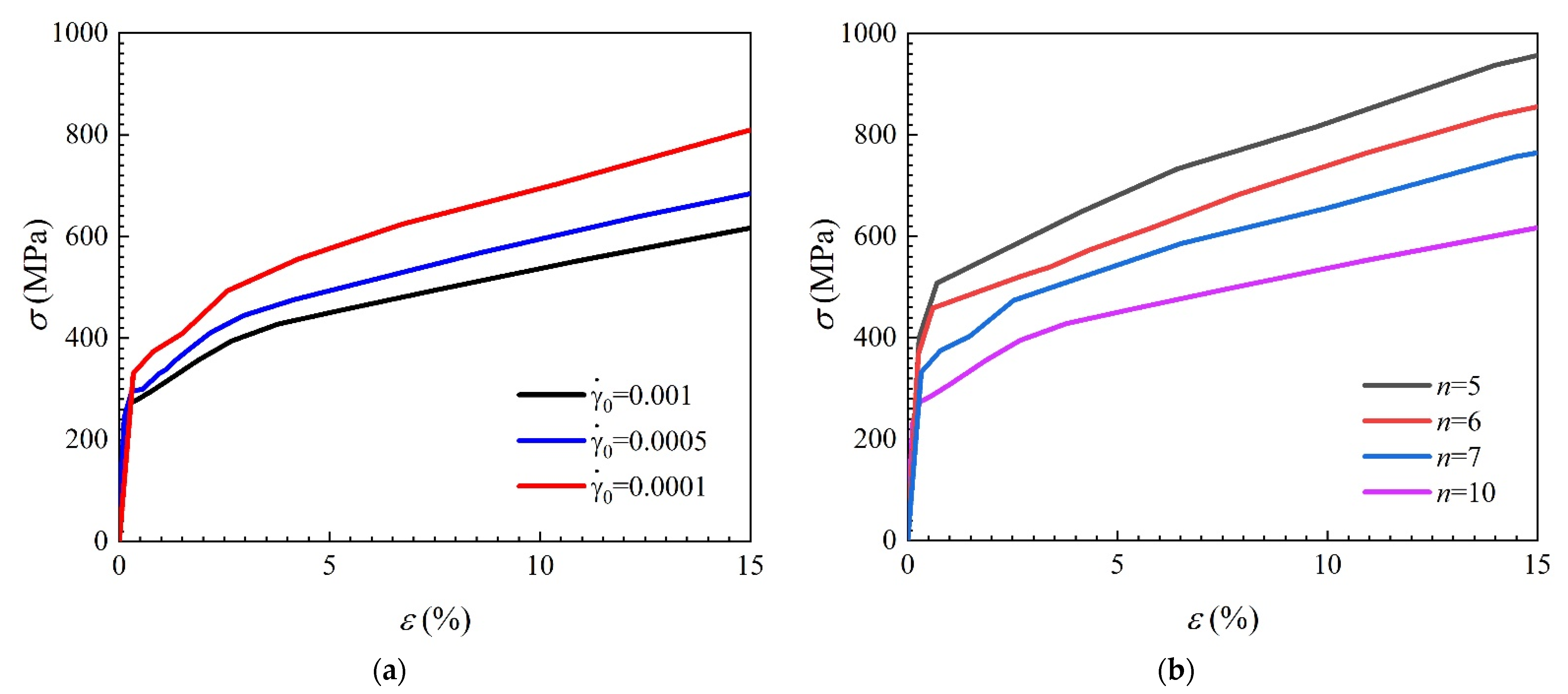
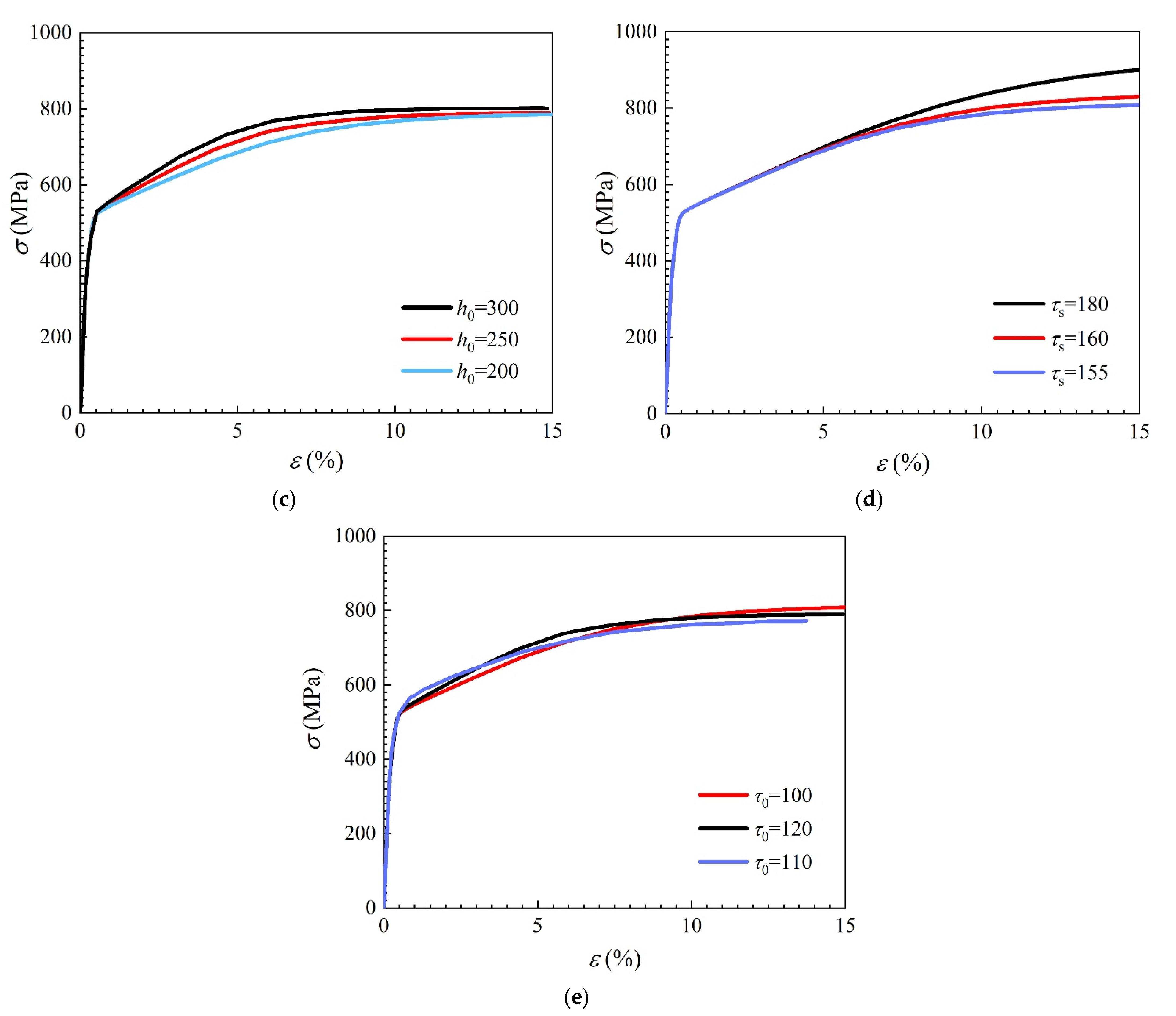
Using several trials of these parameters, the stress-strain curves can be simulated as shown in Figure 5. The rate sensitive parameter n affects the yield strength of the material. During the tensile process, the smaller n is, the more stress is required to reach the yield state. The reference shear rate affects the plastic hardening process of the crystal. With the decrease of , the material shows much more obvious hardening behaviors. The hardening modulus h0 does not affect the ultimate strength, but the strength becomes more stable easily with a large modulus. The initial slip system strength and the saturated critical partial shear stress affect the hardening process. The strength increases with the shear stress of the critical part , while the initial flow stress shows an opposite feature.
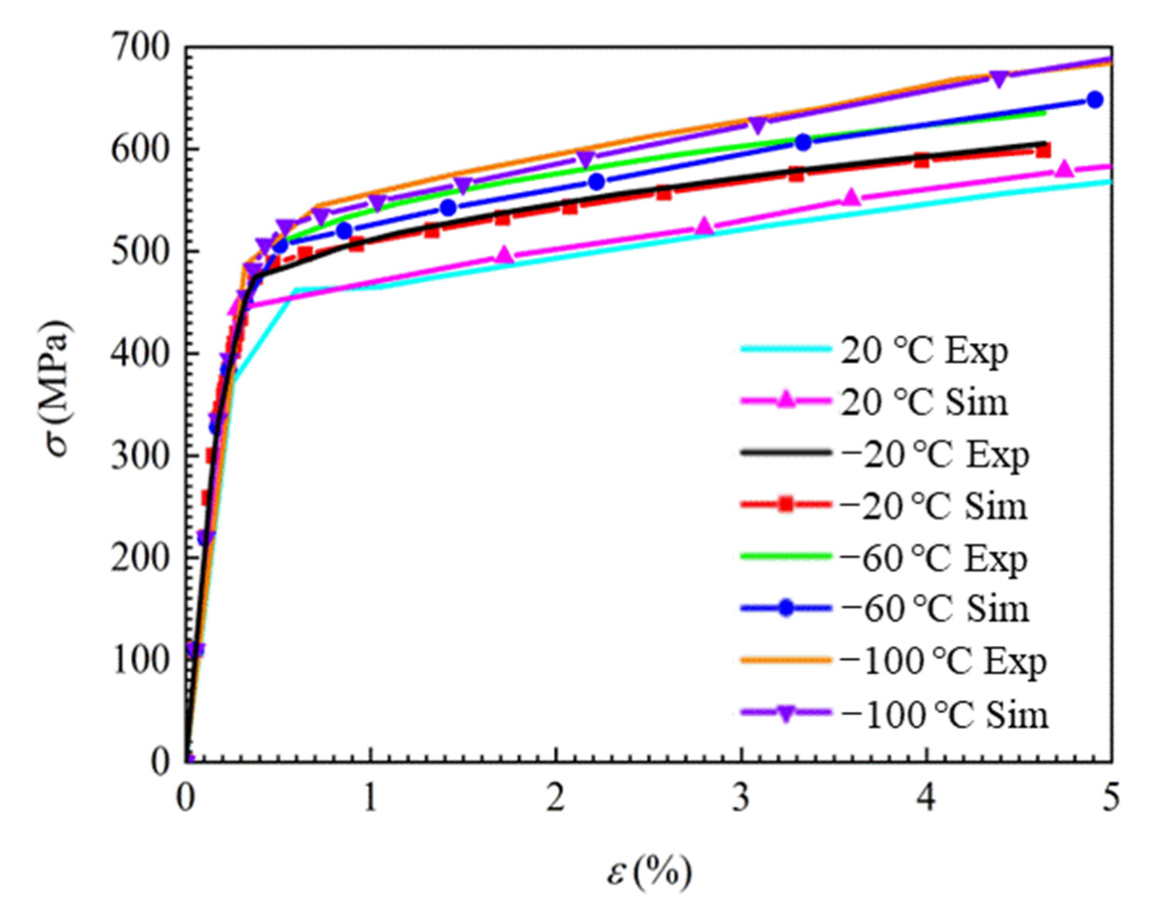
The trial-and-error method obtained the simulation results and compared them with the test results [14], as shown in Figure 6. The test stress in the figure is compared with Cauchy stress. It can be seen from the figure that the tensile simulation results are consistent with the experimental results within the strain range of 5%, which indicates that the CPFEM can better simulate the uniaxial tensile process of SA508-III steel. The material parameters of the crystal plasticity model are finally determined in Table 3. The simulated stress field is shown in Figure 7. It can be obviously found that the concentrated stress presents near the grain boundary.
4. Fracture Tests and Simulation
4.1. Material
In this research, the fracture toughness of SA508-III steel was tested, and other elements in the material except Fe are shown in Table 4. The material is utilized after normalizing, quenching, high temperature tempering, and other heat treatment process, which was transformed into austenite at 880 °C and held for 10.5 h. Then the material was quenched by water spray, tempered at 660 °C for 10 h, and finally cooled to room temperature in air [31].
4.2. Fracture Tests
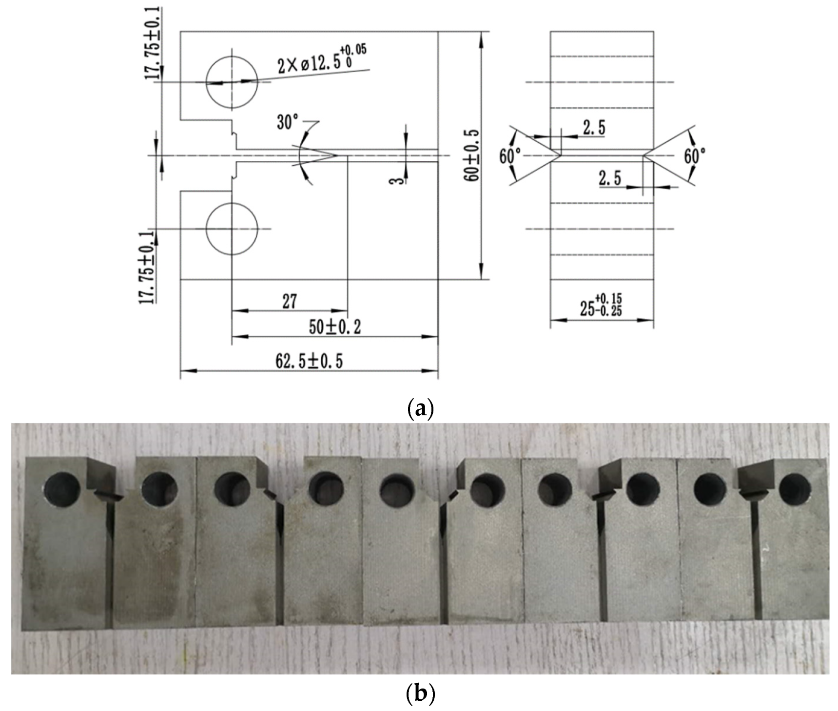
The fracture toughness tests of 1-inch standard compact tensile samples (1T-CT) were conducted according to American Society of Testing Materials E1820-17 (ASME E1820-17) [32]. The design parameters and physical figure of 1T-CT sample are shown in Figure 8. The side grooves were processed on both sides. The depth of the side grooves is 20% of the thickness (10% of each thickness on both sides), adopting the recommended value of ASTM E1820-17.
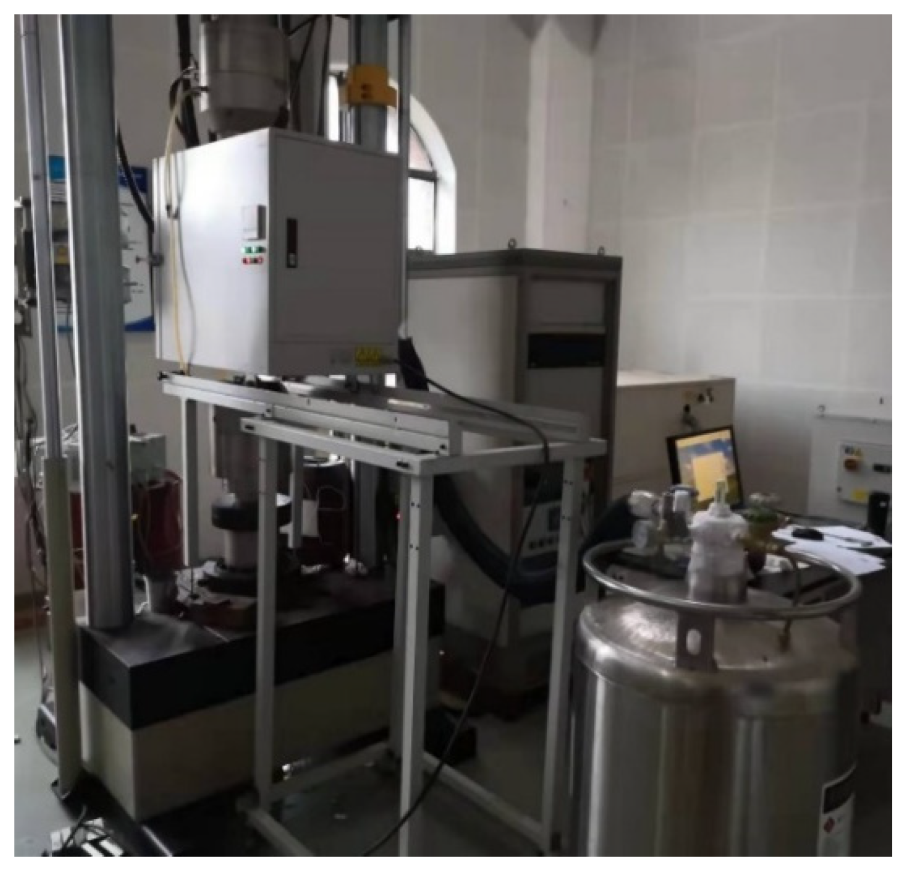
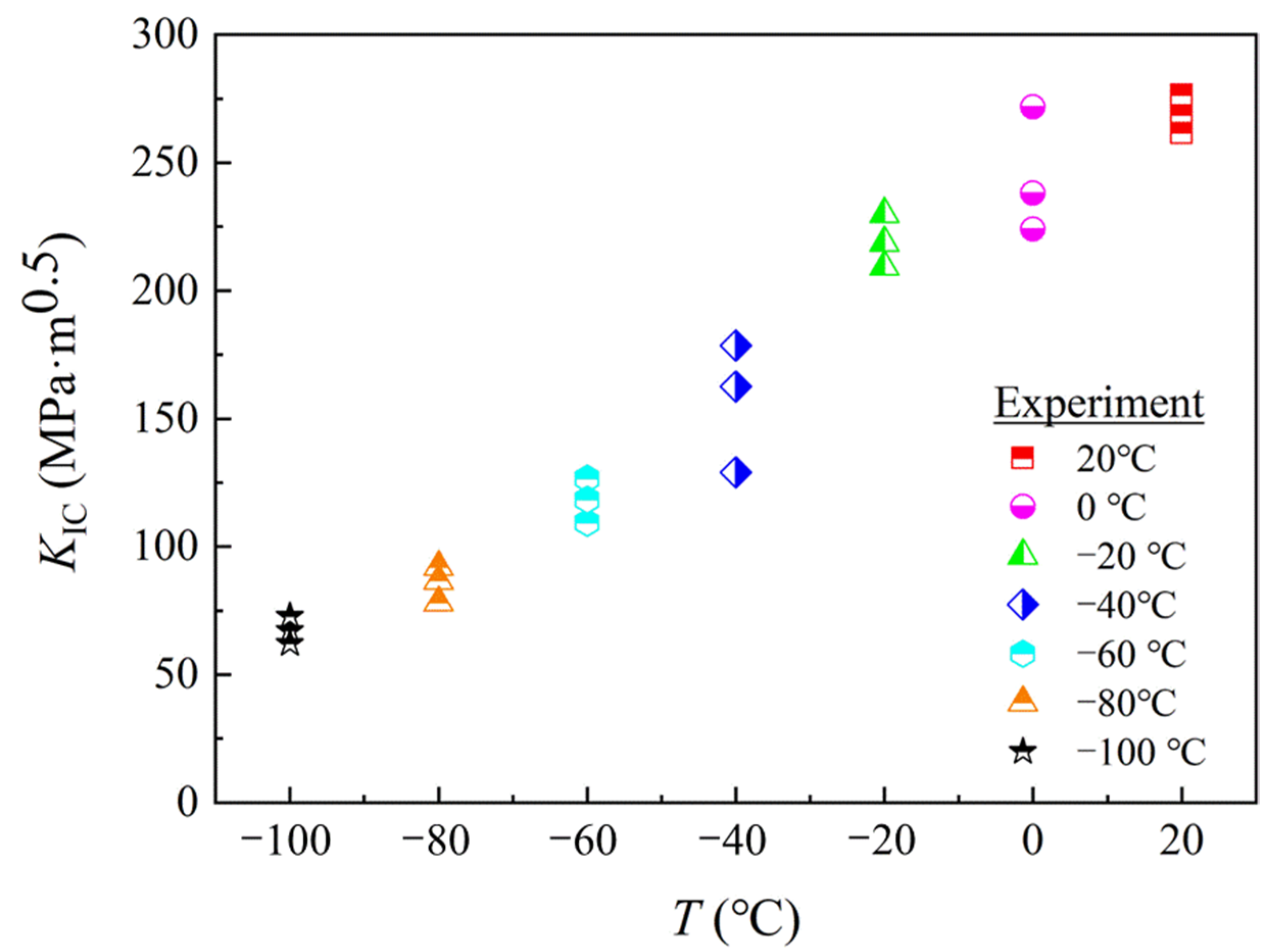
The fracture toughness test was carried out on an Instron 8850 test machine (Instron Corporation, Canton, OH, USA) with a cryostat cooled by liquid nitrogen, as shown in Figure 9. The test temperature ranges from −100 °C to 20 °C, with one temperature point set every 20 °C. Before the experiment, the sample was cooled for 30 min, so that the sample was fully cooled. The test results at different temperatures are shown in Figure 10.
4.3. Crack Tip Stress Distribution
Using the material parameters of crystal plasticity constitutive model calibrated in Section 2, the crack models were established to obtain the stress field. The Voronoi model is also utilized to create a crystal plasticity finite element model when creating a crack model of CT specimen. A 2D half CT model was established with assuming the plane strain condition. To simulate the effect of grain, a crack tip fracture zone with 1 × 0.5 mm2 was considered with real grain characterize. The other part outside the zone was coarse-grained for reducing the process of calculation. According to Liu [14], modeling with large grains outside the crack tip has little influence on the calculation of the whole model. The grains in the zone at the crack tip were refined and simulated. The symmetry restrictions in the Voronoi model of the CT samples were imposed. The configuration and load of the 0.5-inch CT (0.5T-CT) model and the 1-inch CT (1T-CT) model were similar.
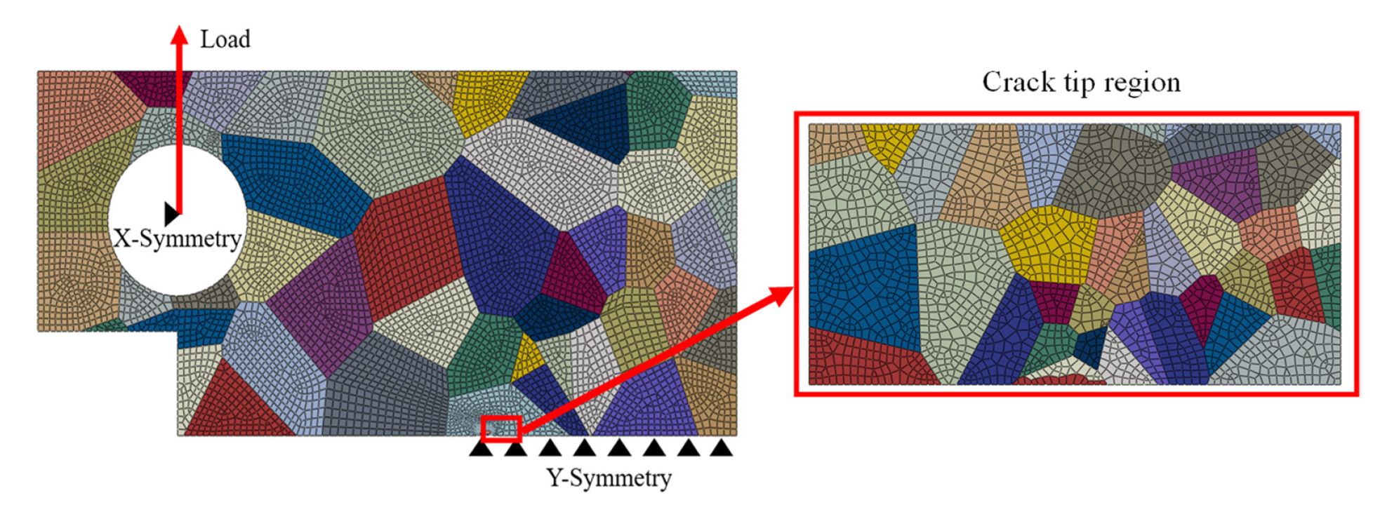
The Voronoi model and boundary conditions of a 1T-CT sample are described in Figure 11. A symmetry constraint was applied on the crack line with the Y direction. To ensure the displacement in Y direction during loading, a displacement constraint in the X direction at the center of the hole which coupled the node on the hole line. A force was applied to the center of the circular hole. The crack tip region contained 38 grains with elements of 2480.
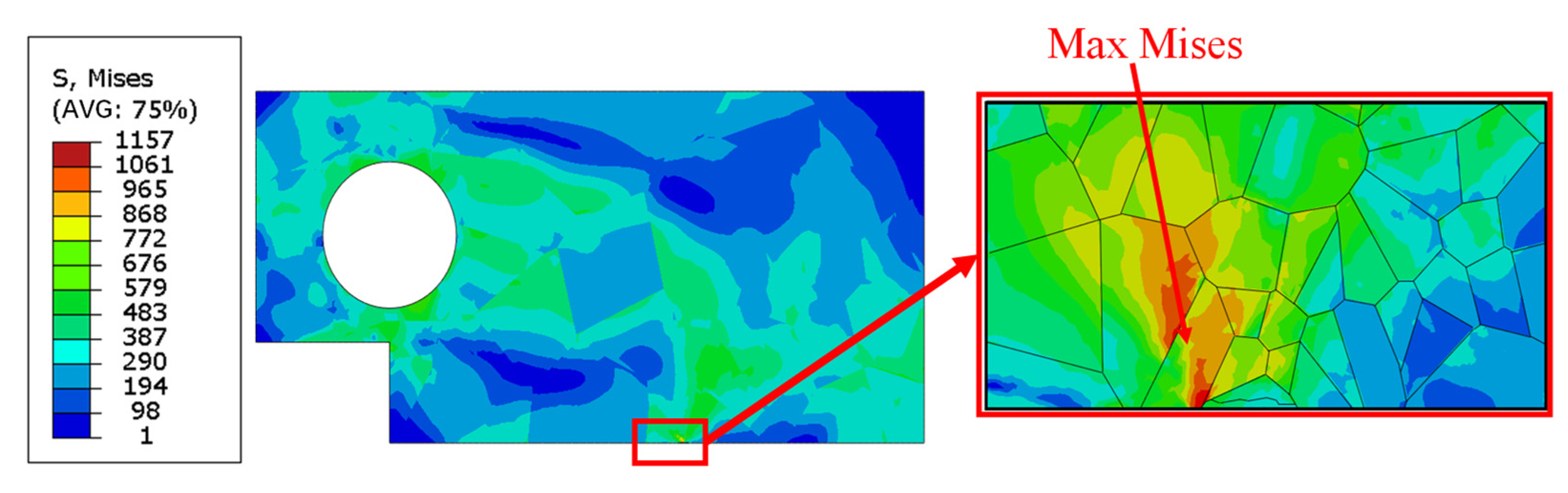
The computed stress distribution of the CT model was shown in Figure 12, exhibiting the overall model and the stress field at the crack tip. Moreover, the image of the crack tip area is enlarged to observe of the grain deformation after deformation. It can be obviously found that the stress concentration occurred on the grain boundary.
4.4. Beremin Local Approach to Cleavage Fracture
The CPFEM simulates the mechanical behavior of materials from a microscopic point of view, and the Beremin local approach to cleavage fracture is a microscopic mathematical model method of fracture toughness based on stress field. Therefore, this study introduced the Beremin local approach to cleavage fracture combined with the CPFEM to study the fracture toughness of SA508-III steel at different temperatures.
The formula of Beremin’s [17] cleavage fracture probability is expressed by the following:
where is Weibull stress which can be determined by the stress field and is the driving force of cleavage fracture. and m are the characteristic parameters of the local cleavage fracture method, and they are both boundary or load independent material constants. m is Weibull slope, which is related to the size distribution of microcracks in ferritic steel. is the quantity reflecting the microscopic toughness of the material, which is equal to the value of when = 0.63.
Weibull stress can be calculated using the maximum principal stress by the following:
where is the volume of the ith element in the crack tip, and is the maximum principal stress on ; is the total number of mesh elements in the crack tip; is the reference volume used to reflect the microstructure of materials, and the reference value of this research is 0.000125 mm3.
There are many parameter calibration methods for the Beremin model [17], such as the Minami calibration method, the TSM calibration method, etc. The above methods all have certain shortcomings and deficiencies. This work applied the m- curve intersection calibration method to calibrate the Beremin parameters proposed by Cao [21]. This method is a simplification of the above method. It only needs to intersect the m- curves of samples with different restraint degrees, and the intersection of the curves is the calibrated m and values. According to the integrity assessment standard R6 [33] of defective structures, the cleavage local fracture characteristic parameter m of most nuclear steels is between 10 and 60.
To study the fracture toughness of SA508-III steel, the sample size used in this research with 1T-CT sample and 0.5T-CT sample to calibrate the parameters. In order to obtain the m- characteristic curve, the corresponding parameter calibration calculation process has the following steps:
- (1)
- Create CT specimen models with difference constraints, using CPFEM;
- (2)
- Obtain the fracture toughness scale parameter of 1T-CT and 0.5T-CT, and , based on the existing fracture toughness experimental data with two different restraints;
- (3)
- Assuming multiple values of m, the force F can be determined when the corrected test results equal to or . Then substituting it into the CPFEM model, Weibull stress can be calculated. One can get , while . two m- characteristic curves can be obtained, and the intersection of the characteristic curves is the m value and obtained.
According to the research [34], the fracture toughness scale parameter of 1T-CT and 0.5T-CT at T = −60 °C can be calculated by:
where N is the number of existing experimental data; is the fracture toughness value obtained in the experiment; is the minimum value of fracture toughness, = 20 MPa·m0.5. Through calculation: = 100.67 MPa·m0.5, = 118.39 MPa·m0.5.
According to the standard ASME E1820-17, the relationship between the fracture toughness and the load F of the CT sample can be obtained.
Due to the elastic plastic behavior of SA508-III, the fracture toughness should be corrected by fracture surface energy. The study of Mathieu [17,35] shows that the fracture surface energy is related to temperature, so the temperature variable is introduced to correct the fracture toughness based on the study of Griffth [36]. According to the definition of stress intensity factor , the conversion relationship between stress intensity factor and fracture toughness with temperature T as a variable is obtained, as shown in Equation (12).
5. Discussions
5.1. Parameter Calibration
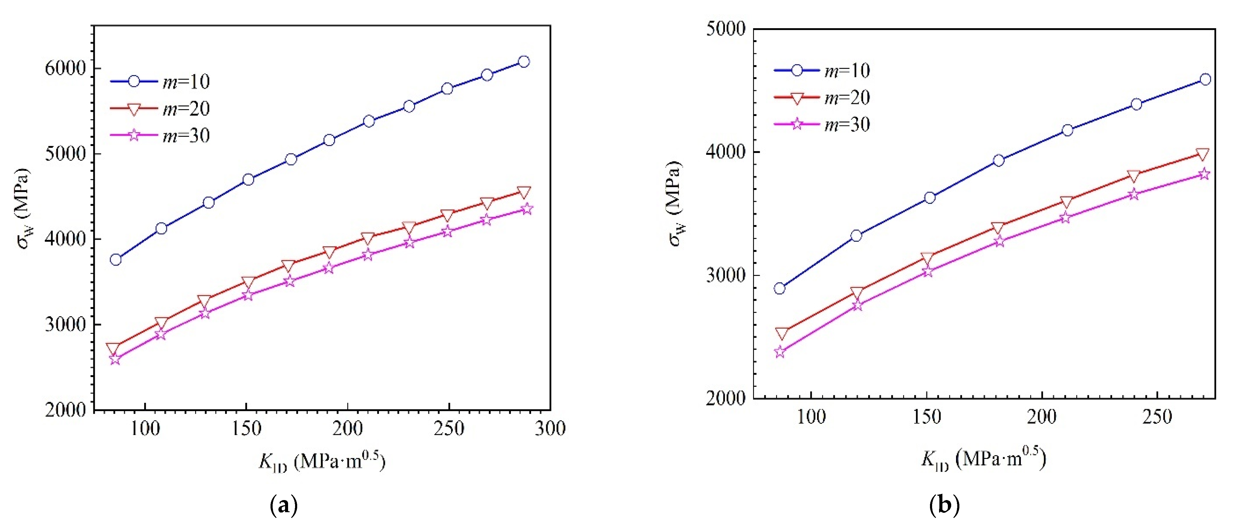
The relation between Weibull stress and m can be obtained according to the above modified formula. The calculation of Weibull stress is completed by a Python program [37]. The results of fracture toughness and Weibull stress varying with m are shown in Figure 13. It can be seen from the figure that the Weibull stress decreases as the increase of m value under the same load.
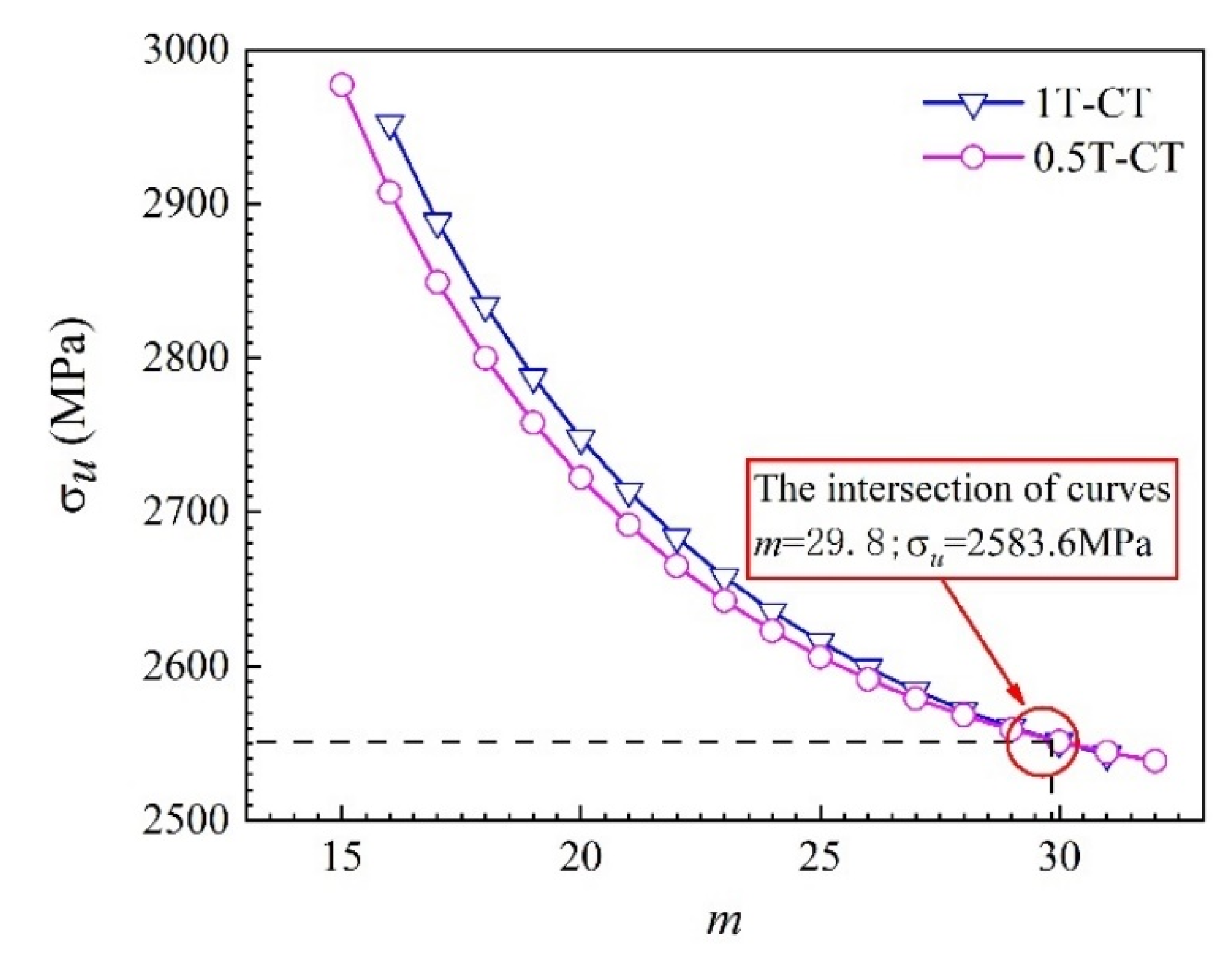
Meanwhile, the corresponding force F of the 1T-CT sample and the 0.5T-CT sample at −60 °C can be obtained by the Equation (11), = 48.75 kN, = 9.36 kN. Then, we can calculate the stress and strain field under these loads for the CT models with the CPFEM. With the assumption of a series values of m, Weibull stress is evaluated and plotted in Figure 14. The intersection of the two curves in the figure is the required m, indicating that the fracture toughness of the 1T-CT sample and the fracture toughness of the 0.5T-CT sample can be better converted at this value. Rounding and correcting the values of m and , the final related parameters are determined as m = 30, = 2590 MPa. Moreover, there is little difference between this study and the results obtained by Zhou [38] with m = 31 and = 2520 MPa. Therefore, the fracture probability model of SA508-III steel obtained by Beremin local approach model can be written as:
5.2. Prediction of Fracture Toughness
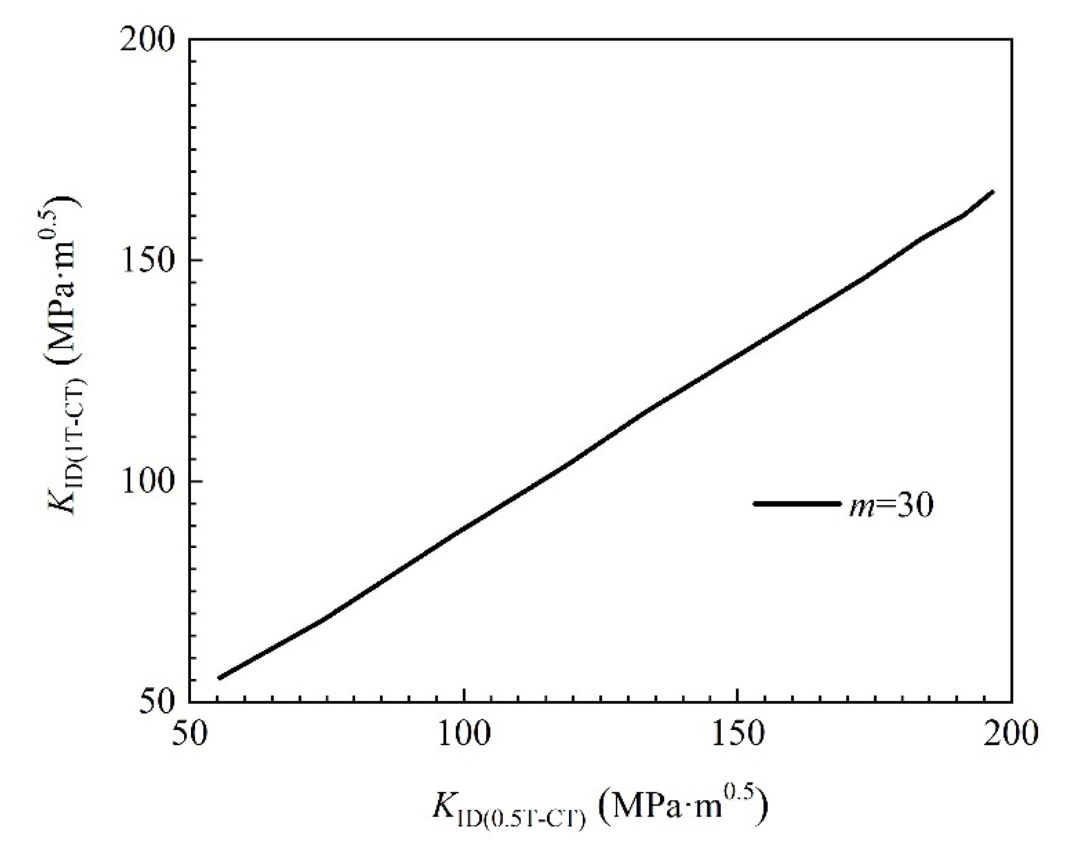
After obtaining m = 30, the fracture toughness values of the 1T-CT sample and the 0.5T-CT sample were converted, and the conversion results are shown in Figure 15. It can be seen from the figure that the transformation curve can be approximately regarded as a straight line, indicating that the conversion relationship between the 1T-CT sample and 0.5T-CT sample is linear. The fracture toughness value of the 0.5T-CT sample is usually larger than that of the 1T-CT sample.
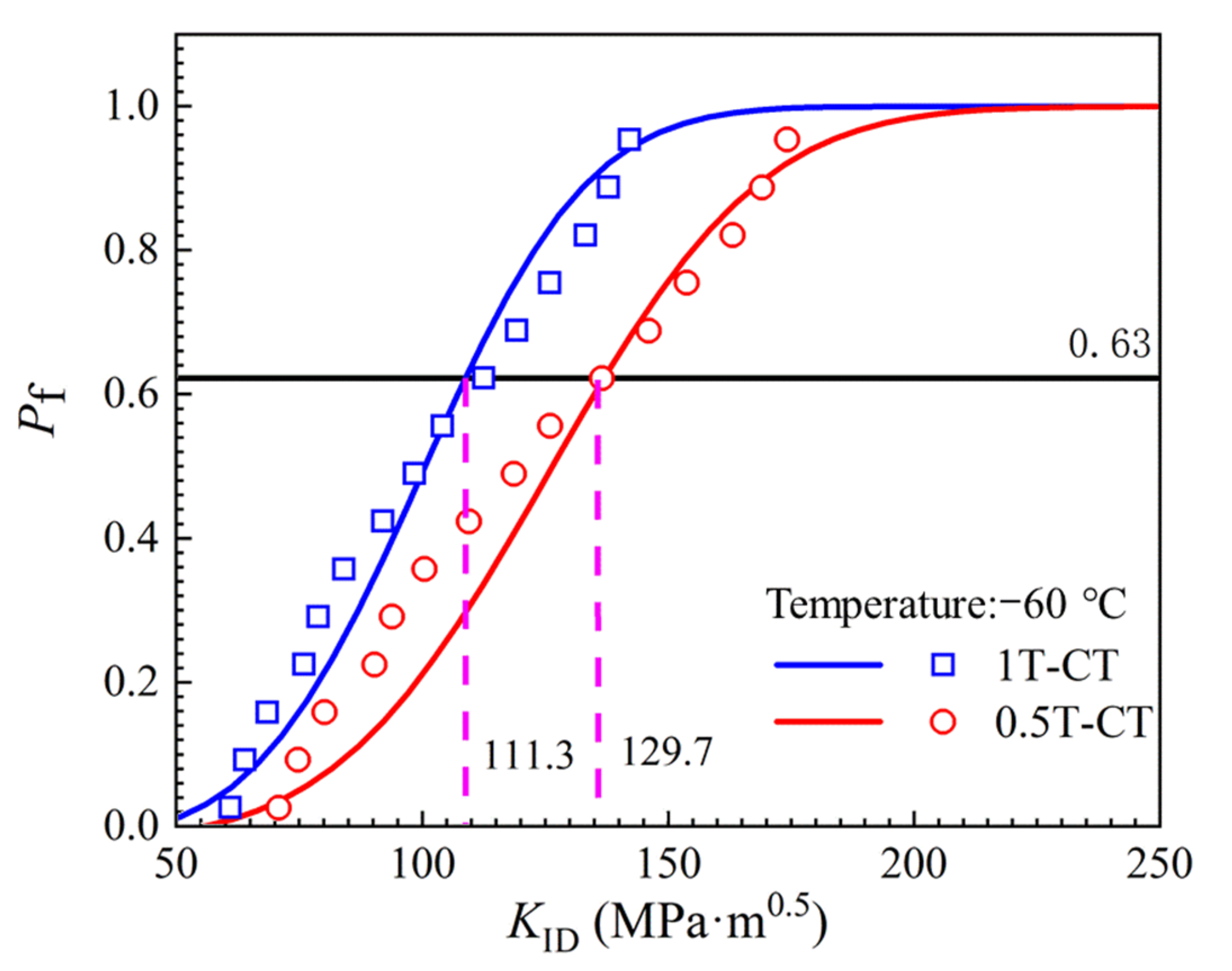
The m and obtained through calibration can be used to calculate the cumulative failure probability as shown in Figure 16. The prediction curve is consistent with test results. Therefore, it can be concluded that the relevant parameters of the Beremin model m = 30, = 2590 MPa can well meet the differences of fracture toughness caused by different constraints. It can be seen from the Figure 15 that when the temperature is −60 °C, the fracture toughness value of the 1T-CT sample is 111.3 MPa·m0.5, and the fracture toughness value of the 0.5T-CT sample is 129.7 MPa·m0.5. The fracture toughness of −20 °C and −100 °C was predicted by the same method after −60 °C. The fracture toughness of −20 °C was 175.9 MPa·m0.5, and that of −100 °C was 65.0 MPa·m0.5.
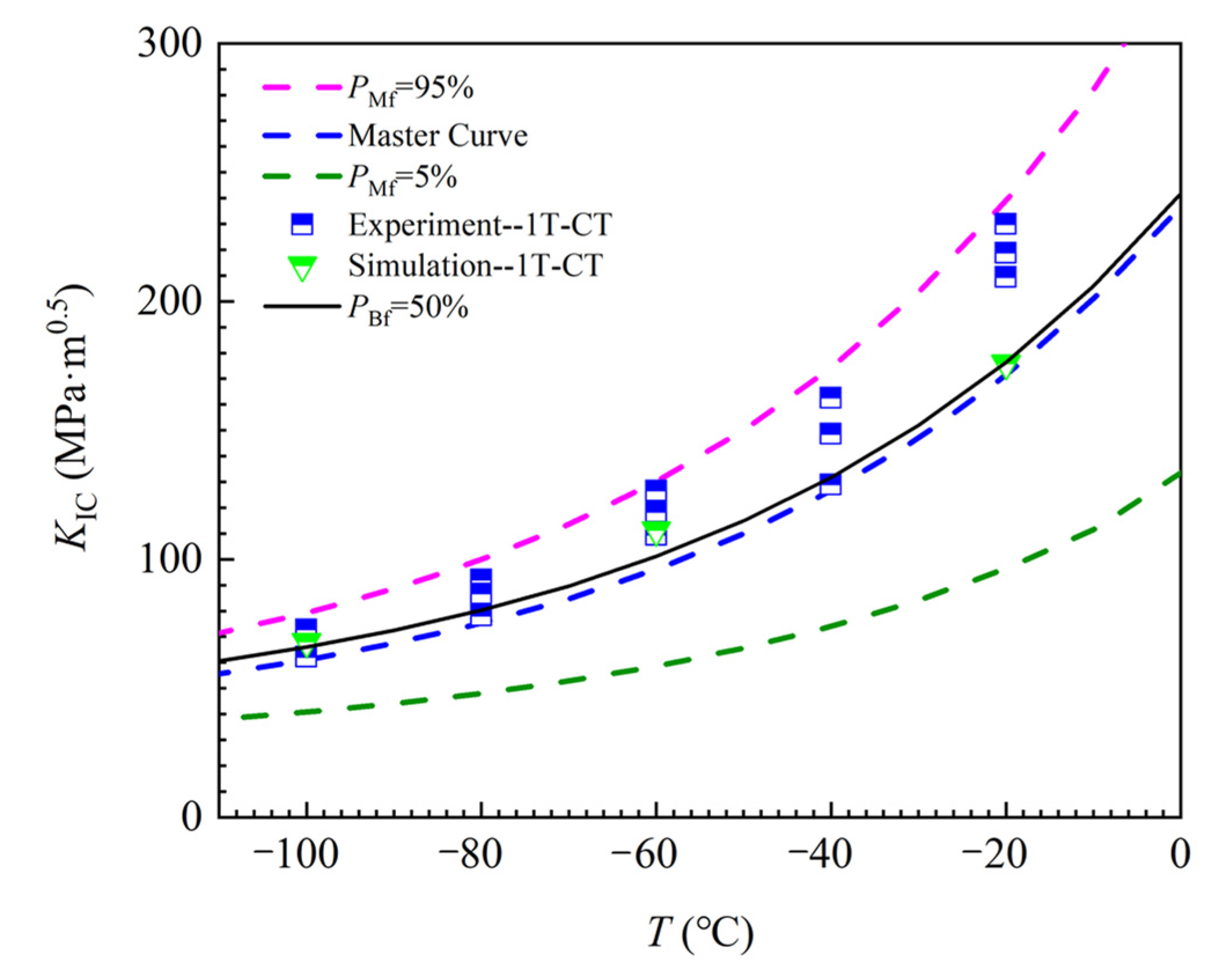
For the temperature dependence of fracture toughness, the master curve method is used in this work. According to the above test, simulation results, and the fracture toughness test data of SA508-III steel obtained by Lee [34], the reference temperature T0 = −63.1 °C is determined, and the master curve can be written as,
The curve with a cumulative failure probability of 50% was obtained based on the calibrated local approach, which was represented by PBf, as shown in Figure 17. The curves with a cumulative failure probability of 5%, 50%, and 95% in the master curve method are also included in Figure 17, which is represented by PMf. In addition, the scatter interval between 5% and 95% is also reduced with temperature. At the same time, the fracture toughness obtained by experiment and simulation in this study is located in the range of 5% curve and 95% curve, but higher than the 50% curve, especially the simulation results of the 0.5T-CT model. The curve with the 50% cumulative failure probability obtained by LA is slightly larger than that obtained by the master curve method, which may be related to the test data used.
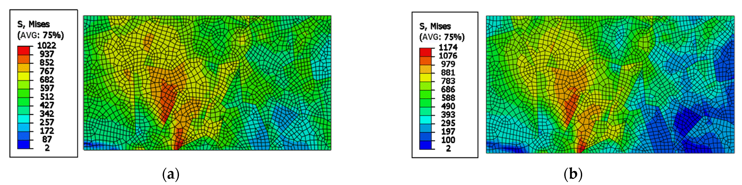
Figure 18 shows the stress results in the crack tip at −20 °C and −100 °C under a load of 43 kN. It can be seen that the stress mainly concentrates on the boundary due to the different orientations of grain. At the same time, the maximum stress at −100 °C is larger than that at −20 °C under the same load, indicating that the material is more prone to fracture at −100 °C than −20 °C under the same load. Meanwhile, it can be seen from the overall stress distribution that the stress distribution at −20 °C is more uniform.
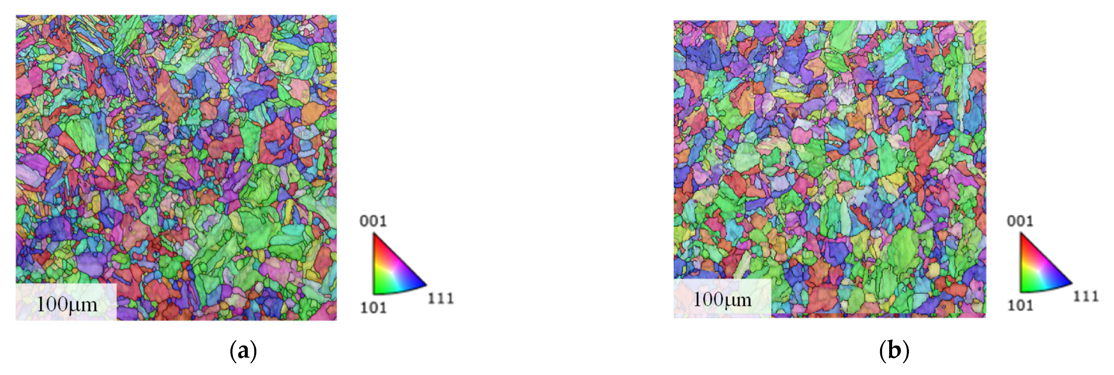
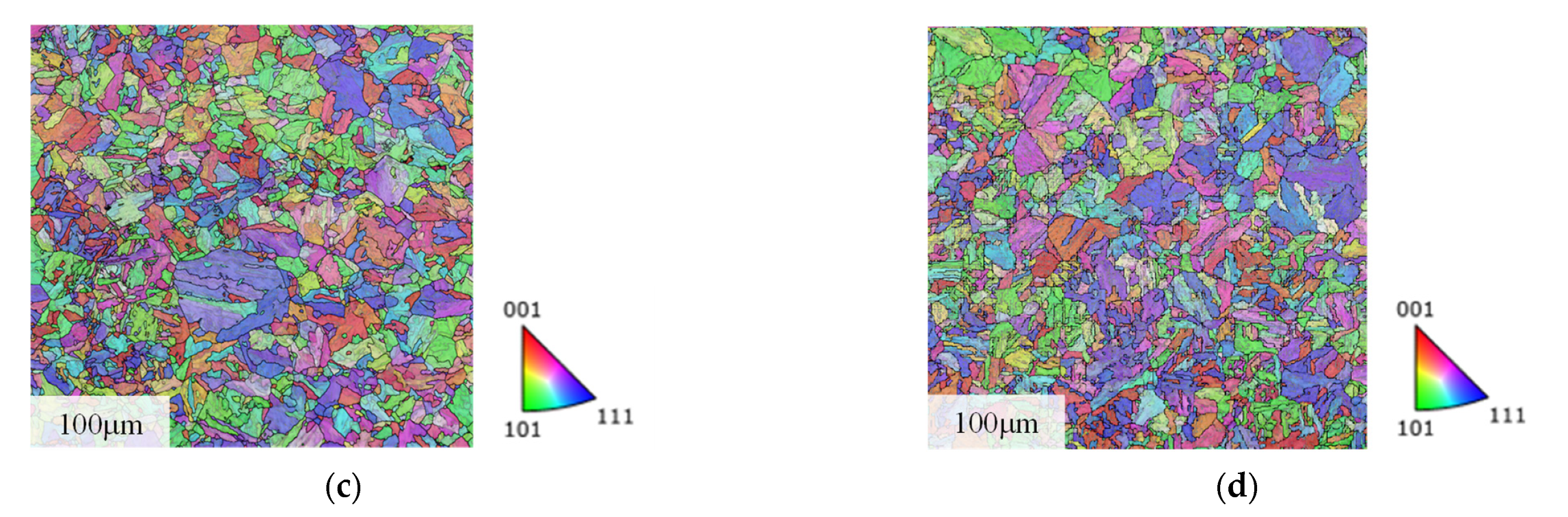
As a material property, the fracture toughness presents scatter, especially under the ductile brittle transition temperature, which is related to the internal grain structure of the material. In order to further illustrate the relationship between fracture toughness and grain orientation, the internal grain information of SA508-III steel at 20 °C, −20 °C, −60 °C, and −100 °C was obtained by electron backscatter diffraction technique, as shown in Figure 19. It can be seen that the grain configuration is not uniform, and the grain orientation distribution is also not consistent at different temperatures. The distribution of colors in the figure indicates the orientation trend of the modified particles. It can be seen that the grains at 20 °C tend to concentrate in the <101> direction, and the grains at −100 °C tend to concentrate in the <111> direction. However, it is still a phenomenon of random distribution as a whole. However, a −20 °C grain orientation and −60 °C grain orientation has no obvious orientation tendency. Combined with the research of Roy [15], it can be concluded that there are certain differences in the changes of different grain orientations and grain shapes of the same material during loading, and the specific orientation of the grains will affect the fracture toughness of the material. The change in the random orientation distribution will influence the material’s fracture toughness. Therefore, the fracture toughness values in the ductile-brittle transition zone are more dispersed.
6. Conclusions
In this research, the fracture toughness of SA508-III steel at different temperatures was studied by using a combination of crystal-plastic finite element and Beremin cleavage fracture local approach model. The following conclusions are drawn:
- (a)
- In order to determine the material parameters in CPFEM, the simulated stress-strain curves are compared with the test results. The calibrated material parameters can agree well with the tensile properties of SA508-III steel at the corresponding temperature.
- (b)
- Several fracture toughness tests were performed at −100 °C to room temperature. The fracture toughness values obtained from the experiment and CPFEM were used to calibrate the relevant parameters of the local method model. Finally, m = 30 and σu = 2590 MPa were obtained, and the fracture toughness conversion between the 0.5T-CT sample and 1T-CT sample was realized.
- (c)
- The cumulative failure probability of fracture toughness was analyzed, and the predicted values of fracture toughness at −20 °C, −60 °C, and −100 °C were obtained when the cumulative failure probability was 0.63. The results show that the predicted fracture toughness values are valid and conform to the Weibull probability distribution.
Author Contributions
Conceptualization, Z.G. and Y.L.; data curation, Z.H.; formal analysis, W.J.; funding acquisition, Y.L.; investigation, Z.H., Y.L., W.J., C.L.; methodology, Z.G.; supervision, Z.G. and Y.L.; writing original draft, Z.H.; writing review and editing, Z.H. and Y.L. All authors have read and agreed to the published version of the manuscript.
Funding
This research was funded by Major National Science and Technology Projects of China, grant number 2017ZX06002006.
Data Availability Statement
Not applicable.
Conflicts of Interest
The authors declare no conflict of interest.
References
- ASME XI: Rules for Inservice Inspection of Nuclear Power Plant Components; American Society of Mechanical Engineers: New York, NY, USA, 2017.
- Miller, M.K.; Burke, M.G. An atom probe field ion microscopy study of neutron irradiated pressure vessel steels. J. Nucl. Mater. 1992, 195, 68–82. [Google Scholar] [CrossRef]
- Brimbal, D.; Decamps, B.; Barbu, A. Dual-beam irradiation of α-iron: Heterogeneous bubble formation on dislocation loops. J. Nucl. Mater. 2011, 418, 313–315. [Google Scholar] [CrossRef]
- Domain, C.; Becquar, C.S.; Maplerba, L. Simulation of radiation damage in Fealloys: An object kinetic Monte Carlo approach. J. Nucl. Mater. 2004, 335, 121–145. [Google Scholar] [CrossRef]
- Song, Y.X.; Ma, Y.; Chen, H.F.; He, Z.B.; Chen, H.; Zhang, T.H. The effects of tensile and compressive dwells on creep-fatigue behavior and fracture mechanism in welded joint of P92 steel. Mater. Sci. Eng. A 2021, 813, 141129. [Google Scholar] [CrossRef]
- Taylor, G.I. Plastic strain in metals. J. Inst. Met. 1938, 307, 62. [Google Scholar]
- Hill, R.; Rice, J.R. Constitutive analysis od elastic-plastic crystals at arbitrary strain. J. Mech. Phys. Solids. 1972, 20, 401–413. [Google Scholar] [CrossRef]
- Peirce, D.; Asaro, R.J.; Needleman, A. An analysis of nonuniform and localized deformation in ductile single crystals. Acta Metall. 1982, 30, 1087–1119. [Google Scholar] [CrossRef]
- Vorono, G. Nouvelles applications des parametres countinus a la theorie des forms quadratiques. Deuxieme memoire: Recherches sur les parallelloedres primitifs. J. Reine. Angew. Math. 1908, 134, 198–287. [Google Scholar] [CrossRef]
- Wan, Q.; Shu, G.; Wang, R.; Ding, H. Study on microstructure evoltion of SA508-3 steel under proton irradiation. Acta Metall. Sin. 2012, 48, 929–934. [Google Scholar] [CrossRef]
- Li, Y.; Zhou, M. Prediction of fracture toughness of ceramic composites as function of microstructure: I. numerical simulations. J. Mech. Phys. Solids. 2013, 61, 472–488. [Google Scholar] [CrossRef]
- Li, Y.; Zhou, M. Prediction of fracturess toughness of ceramic composites as function of microstructure: II. analytical model. J. Mech. Phys. Solids. 2013, 61, 489–503. [Google Scholar] [CrossRef]
- Vincent, L.; Libert, M.; Marini, B.; Rey, C. Towards a modelling of RPV steel brittle fracture using crystal plasticity computations on polycrystalline aggregates. J. Nucl. Mater. 2010, 406, 91–96. [Google Scholar] [CrossRef]
- Liu, Y.P.; Nie, J.F.; Lin, P.D.; Liu, M.D. Irradiation tensile property and fracture toughness evaluation study of A508-3 steel based on multi-scale approach. Ann. Nucl. Energy 2020, 138, 107157. [Google Scholar] [CrossRef]
- Chen, L.R.; Liu, W.B.; Yu, L.; Cheng, Y.Y.; Ren, k.; Sui, H.N.; Yi, X.; Duan, H.L. Probabilistic and constitutive models for ductile-to-brittle transition in steels: A competition between cleavage and ductile fracture. J. Mech. Phys. Solids. 2020, 135, 103809. [Google Scholar] [CrossRef]
- Roy, U.; McDowell, D.L.; Zhou, M. Effect of grain orientations on fracture behavior of polycrystalline metals. J. Mech. Phys. Solids. 2021, 151, 104384. [Google Scholar] [CrossRef]
- Beremin, F.M.; Pineau, A.; Mudry, F. A local approach to cleavage fracture of nuclear pressure vessel steel. Metall. Trans. 1983, 14, 2277–2287. [Google Scholar] [CrossRef]
- Mathieu, J.P.; Inal, K.; Berveiller, S.; Diard, O. A micromechanical interpretation of the temperature dependence of Beremin model parameters for french RPV steel. J. Nucl. Mater. 2010, 406, 97–112. [Google Scholar] [CrossRef] [Green Version]
- Qian, G.A.; Lei, W.S. A statistical model of fatigue failure incorporating effects of specimen size and load amplitude on fatigue life. Philos. Mag. 2019, 99, 2089–2125. [Google Scholar] [CrossRef] [Green Version]
- Qian, G.A.; Lei, W.S.; Niffenegger, M.; Gonzalez, V.F. On the temperature independence of statistical model parameters for cleavage fracture in ferritic steels. Philos. Mag. 2018, 98, 959–1004. [Google Scholar] [CrossRef] [Green Version]
- Cao, Y.P.; Hui, H.; Wang, G.Z.; Xuan, F.Z. Inferring the temperature dependence of Beremin cleavage model parameters from the Master Curve. Nucl. Eng. Technol. 2011, 241, 29–45. [Google Scholar] [CrossRef]
- Chang, Y.S.; Kim, J.M.; Ko, H.O. Experimental and numerical investigations on brittle failure probability and ductileresistance property. Int. J. Pres. Ves. Pip. 2005, 85, 647–654. [Google Scholar] [CrossRef]
- Roters, F.; Eisenlohr, P.; Hantcherli, L.; Tjahjanto, D.D.; Bieler, T.R.; Raabe, D. Overvive of constitutive laws, kinematics, homogenization and multiscale in crystal plasticity finite-element modeling: Theory, experiments, applications. Acta Mater. 2010, 58, 1152–1211. [Google Scholar] [CrossRef]
- Asaro, R.J. Micromechanics of crystals and pilycrystals. Adv. Appl. Mech. 1983, 23, 1–115. [Google Scholar]
- Zhang, C.; Zhang, W.L.; Shen, W.F.; Xia, Y.N.; Yan, Y.T. 3D Crystal Plasticity Finite Element Modeling of the Tensile Deformation of Polycrystalline Ferritic Stainless Steel. Acta. Metall. Sin. 2017, 30, 79–88. [Google Scholar] [CrossRef] [Green Version]
- Tikhovskiy, I.; Raabe, D.; Roters, F. 159 A practical method for simulation of deep cup-drawing based on crystal plasticity model. Scr. Mater. 2006, 54, 1537. [Google Scholar] [CrossRef]
- He, X.K.; Bai, T.; Liu, Z.D. Effect of Heating Rate and Cooling Mode on Austenite Grain Size of 508-3 Steel. Hot Work. Technol. 2013, 42, 204–205. [Google Scholar]
- ASTM E8/E8M-16ae1; Standard Test Methods for Tension Testing of Metallic Materials. ASTM International: West Conshohocken, PA, USA, 2017.
- Huang, Y.G. A User-Material Subroutine Incorporating Single Crystal Plasticity in the ABAQUS Finite Element Program; Harvard: Harvard University Report, MECH178; Harvard University: Cambridge, MA, USA, 1991. [Google Scholar]
- Raabe, D.; Wang, Y.; Roters, F. Crystal Plasticity Simulation Study on the Influence of Texture on Earing in Steel. In Proceedings of the 3 Computational Microstructure Evolution in Steels: Papers from Symposium of the Materials Science and Technology 2004 Meeting, New Orleans, LA, USA, 26–30 September 2005; Elsevier: Amsterdam, The Netherlands, 2005; p. 221. [Google Scholar]
- Ahn, Y.S.; Kim, H.D.; Byun, T.S.; Oh, Y.J.; Kim, G.M.; Hong, J.H. Application of intercritical heat treatment to improve toughness of SA508 Cl. 3 reactor pressure vessel steel. Nucl. Eng. Technol. 1999, 194, 161–177. [Google Scholar] [CrossRef]
- ASTM E1820; Standard Test Method for Measurement of Fracture Toughness. ASTM International: New York, NY, USA, 2018.
- Cai, L.X.; Liu, Y.J.; Ye, Y.M.; Niu, Q.Y. Uniaxial Ratcheting Behavior of Stainless Steels: Experiments and Modeling. Key. Eng. Mater. 2004, 274–276, 823–828. [Google Scholar] [CrossRef]
- Lee, B.S.; Kim, M.C.; Kim, M.W.; Yoon, J.H.; Hong, J.H. Master curve techniques to evaluate an irradiation embrittlement of nuclear reactor pressure vessels for a long-term operation. Int. J. Pres. Ves. 2008, 85, 593–599. [Google Scholar] [CrossRef]
- Mathieu, J.P. Analyse et Modélisation Micromécanique du Comportement et dela Rupture Fragile de L’acier 16MND5: Prise en Compte des Hétérogénéités Microstructurales. Ph.D. Thesis, ENSAM Metz, Metz, France, 2006. [Google Scholar]
- Griffith, A.A. The phenomena of rupture and flow in solids. Philos. Trans. R. Soc. Lond. 1920, 221, 163–198. [Google Scholar]
- Li, Y.B.; Zhu, L.Y.; Zhou, M.J.; Lei, Y.B.; Wang, W.H.; He, Z.B.; Gao, Z.L. Weibull stress solutions for 2D cracks under mode II loading. Int. J. Fract. 2020, 225, 31–45. [Google Scholar] [CrossRef]
- Zhou, H.H.; Zhong, W.H.; Ning, G.S.; Liu, H.; Yang, W. Size effect on fracture toughness of A508-3 steel predicted by using beremin model. At. Energy Sci. Technol. 2022, 56, 185–192. [Google Scholar]
Figure 1.
Grain deformation process.

Figure 2.
Body centroid cubic cell.

Figure 3.
Schematic diagram of 2D Voronoi.

Figure 4.
Voronoi grid diagram and boundary conditions simulated by tensile test.

Figure 5.
Comparison of the effects of various parameters on the mechanical properties of crystal. (a) Reference shear rate ; (b) rate sensitive parameter n; (c) Initial hardening modulus h0; (d) Saturated critical shear stress ; (e) Initial flow stress .
Figure 5.
Comparison of the effects of various parameters on the mechanical properties of crystal. (a) Reference shear rate ; (b) rate sensitive parameter n; (c) Initial hardening modulus h0; (d) Saturated critical shear stress ; (e) Initial flow stress .


Figure 6.
Comparison between tensile test and simulation results.

Figure 7.
The stress field of the tensile model at −100 °C.

Figure 8.
1T-CT sample. (a) 1T-CT sample design parameters. (b) 1T-CT real sample.

Figure 9.
Experimental equipment.

Figure 10.
Test results.

Figure 11.
Voronoi model and boundary conditions of CT model.

Figure 12.
Calculation results of 40 kN CT model at −100 °C.

Figure 13.
- curve of CT sample (a) 1T-CT sample and (b) 0.5T-CT sample.

Figure 14.
m- curve of 1T-CT and 0.5T-CT samples.

Figure 15.
Fracture toughness conversion curves of 1T-CT and 0.5T-CT samples.

Figure 16.
Cumulative failure probability distribution of fracture toughness of 0.5T-CT sample and 1T-CT sample.
Figure 16.
Cumulative failure probability distribution of fracture toughness of 0.5T-CT sample and 1T-CT sample.

Figure 17.
Master curve of fracture toughness.

Figure 18.
Stress result diagram of crack tip region under 43 kN load (a) −20 °C; (b) −100 °C.

Figure 19.
Information on grain structure of SA508-III steel. (a) 20 °C; (b) −20 °C; (c) −60 °C; (d) −100 °C.
Figure 19.
Information on grain structure of SA508-III steel. (a) 20 °C; (b) −20 °C; (c) −60 °C; (d) −100 °C.


Table 1.
{110} <111> slip system.
| lip plane | 11 | 01 | 10 | 01 | 11 | 10 | 1 | 10 | 10 | 01 | 10 | 10 |
Table 2.
{112} <111> slip system.
| lip plane | 21 | 21 | 11 | 1 | 1 | 21 | 12 | 2 | 2 | 2 | ||
Table 3.
Material parameters used in the simulation model.
| Temperature (°C) | Slip System | C11 (GPa) | C22 (GPa) | C44 (GPa) | h0 (MPa) | n | |||
|---|---|---|---|---|---|---|---|---|---|
| 20 | {110} <111> | 236 | 134 | 119 | 155 | 100 | 65 | 5 | 0.001 |
| −20 | {112} <111> | 236 | 134 | 119 | 200 | 130 | 100 | 20 | 0.001 |
| −60 | {112} <111> | 236 | 134 | 119 | 200 | 140 | 100 | 17 | 0.001 |
| −100 | {112} <111> | 236 | 134 | 119 | 200 | 155 | 100 | 15 | 0.001 |
Table 4.
SA508-III steel composition. (wt%, mass fraction).
| Element | C | Si | Mn | Ni | Cr | Mo | P | S | Cu | V |
|---|---|---|---|---|---|---|---|---|---|---|
| Content | 0.240 | 0.081 | 1.350 | 0.820 | 0.160 | 0.510 | 0.008 | ≤0.001 | 0.017 | 0.003 |
Publisher’s Note: MDPI stays neutral with regard to jurisdictional claims in published maps and institutional affiliations. |
© 2022 by the authors. Licensee MDPI, Basel, Switzerland. This article is an open access article distributed under the terms and conditions of the Creative Commons Attribution (CC BY) license (https://creativecommons.org/licenses/by/4.0/).
Share and Cite
MDPI and ACS Style
He, Z.; Li, C.; Li, Y.; Jin, W.; Gao, Z. Prediction of Fracture Toughness Scatter Based on Weibull Stress Using Crystal Plasticity Finite Element Method. Metals 2022, 12, 872. https://0-doi-org.brum.beds.ac.uk/10.3390/met12050872
AMA Style
He Z, Li C, Li Y, Jin W, Gao Z. Prediction of Fracture Toughness Scatter Based on Weibull Stress Using Crystal Plasticity Finite Element Method. Metals. 2022; 12(5):872. https://0-doi-org.brum.beds.ac.uk/10.3390/met12050872
Chicago/Turabian StyleHe, Zhibo, Chen Li, Yuebing Li, Weiya Jin, and Zengliang Gao. 2022. "Prediction of Fracture Toughness Scatter Based on Weibull Stress Using Crystal Plasticity Finite Element Method" Metals 12, no. 5: 872. https://0-doi-org.brum.beds.ac.uk/10.3390/met12050872
Note that from the first issue of 2016, this journal uses article numbers instead of page numbers. See further details here.