
Energy Performance Evaluation of Historical Building


Department of Building Engineering, Energy Systems, and Sustainability Science, Faculty of Engineering and Sustainable Development, University of Gävle, 801 76 Gävle, Sweden
*
Author to whom correspondence should be addressed.
Buildings 2022, 12(10), 1667; https://0-doi-org.brum.beds.ac.uk/10.3390/buildings12101667
Submission received: 9 September 2022
/
Revised: 22 September 2022
/
Accepted: 9 October 2022
/
Published: 12 October 2022
(This article belongs to the Section Building Energy, Physics, Environment, and Systems)
Abstract
:Retrofitting measures in old buildings aimed at reducing energy usage have become important procedures meant to counteract the effects of climate change and greenhouse gas emissions. The aim of this study is to evaluate energy usage, thermal comfort, and CO2 emissions of an old building by changing parameters such as building orientation, shading systems, location, low energy film application, and alternative energy supply in the form of a geothermal heat pump. When evaluating the buildings in terms of geographical location with or without applying the low energy film, the results show that the city of Gävle in Sweden requires the most heating energy, 150.3 kWh/m2∙year (B0) compared to Jakarta (L0), which requires 23.8 kWh/m2∙year. When examining the thermal comfort, cases B4 and L4 demonstrate the best results in their respective categories (B0–B4 are cases without low energy film and L0–L4 are cases with applied low energy film). The results for the CO2 emissions levels for B0–B4 and L0–L4 indicate that B4 has the highest value, 400 kg CO2 eq/year higher than B0, and L1 has the lowest value, 731 kg CO2 eq/year lower than B0. The economic feasibility study illustrates that the installation of a geothermal heat pump with at least a coefficient of performance of 4.0 leads to a shorter payback period than solely applying LEF.
1. Introduction
Measures to reduce the energy usage of old buildings have become increasingly necessary due to the importance of lowering the total energy usage in Sweden, especially in the light of global climate change as well as the current energy crisis in Europe. Climate change is one of the most important challenges faced by today’s society. Researchers have shown concerns about the probability of an irreversible transformation of the planet in the near future. The Intergovernmental Panel on Climate Change (IPCC) has collectively agreed that warming of the Earth’s different biospheres was due to an increase in the concentration of greenhouse gases (GHGs) due to anthropogenic activities [1]. Decisions to counter climate change have been the result of international efforts in the Paris Agreement, in Paris COP21 in 2015, and later, in Glasgow COP26 in 2021.
Most global energy usage originates from fossil fuels, such as natural gas, oil, and coal, which are considered harmful to the environment, and consequently, to humans and biodiversity [2]. The primary goal now is to mitigate the effects of global warming and climate change by implementing fast and sustained reductions in GHG emissions; this includes reducing global CO2 emissions by 45% by 2030 to the levels of 2010 [3]. One of the sectors responsible for around 40% of global energy usage is the building sector, which uses mainly non-renewable sources and contributes up to 30% of annual GHG emissions globally [4].
To combat climate change and fossil fuel dependency, it is important to explore possibilities for reducing energy usage and improving the energy efficiency in the existing building stock by means of retrofitting techniques and measures [5]. It has been demonstrated that buildings are affected by global warming during their lifespan due to changes in outdoor conditions that result in a degradation of building energy performance (BEP) and thermal comfort [1]. For this reason, the emissions from the building stock that arise primarily from the demand for space cooling and heating need to be reduced substantially throughout their lifecycle through a dedicated strategy that not only reduces the energy demand through behavioral changes and energy efficiency measures, but also transitions the energy usage toward a reliance on renewable energy sources (decarbonization) [6].
A building can be described as a shelter that protects its inhabitants from the external or surrounding outdoor environment, such as excessive heat (sun), cold, wind, rain, or snow [7]. This establishes an interrelationship between the building and the occupant in the form of interactions with the building envelope, the HVAC system and the occupant’s behavior, operating hours, and number of appliances within the envelope. This interrelationship can lead to high cooling/heating depending on the mentioned parameter configurations, which, in turn, translates into a rise or reduction of the energy demand [7,8].
Morelli et al. [9] retrofitted an old multi-family building from 1896 to reduce the energy usage. Three types of retrofitting measures were implemented, such as installing two different types of interior insulation, retrofitting of windows, and installation of a decentralized mechanical ventilation system with heat recovery. The results illustrated that the retrofit reduced the energy usage from 162.5 kWh/(m2∙year) to 51.5 kWh/(m2∙year), corresponding to 68% reduction of the energy usage. Harrestrup and Svendsen [10] carried out a holistic energy renovation on an old multi-story building with heritage value. The primary focus of the energy-saving measures was to preserve the original architectural expression of the building. The researchers managed to reduce the energy demand by 47%, whereas the theoretical reduction was estimated to be about 39–61%, depending on which room set-point temperature was used (20–24 °C). Curto et al. [11] conducted an energy retrofitting of the Santi Romano Dormitory at Palermo University in Italy. They started with carrying out an energy audit to examine the energy usage, energy load, and other important energy related aspects of the building. Based on the energy audit evaluation, they proposed several retrofit proposals that would reduce the building energy usage; specifically, 65% of the electrical energy and 33% of the thermal energy could be saved by replacing the generation systems, installing a co-generator, replacing windows, and replacing the existing lighting with LED type lighting. Cho et al. [12] proposed several retrofitting measures to improve the energy efficiency and reduce the energy usage of used historic buildings in South Korea. The purposed retrofit package, which had the lowest impact on the historical value, resulted in a 15.9% reduction of the energy usage.
It can also be important to evaluate the building not just from an energy saving point of view, but from a deeper dive into the sustainability of a building, where several considerations are made in terms of the building material and life cycle assessment [13,14].
However, in the current study, the City Hall (Rådhuset) in Gävle, which is used as an office building for the municipality of Gävle, is evaluated for possible energy saving measures, as well as for an energy sensitivity analysis. The main goal in this study is to examine changes in energy performance and thermal comfort by changing various parameters, such as (1) facade orientation (sensitivity analysis), (2) window shadings and low energy film (LEF) (energy saving measure), (3) locations (sensitivity analysis), and (4) alternative energy supply, geothermal heat pump (GHP) (energy saving measure).
The evaluation not only focuses on possible energy saving measures but also on the possibility of this building being in other climate regions as well as having a different facade orientation. This is important due to the possible impending climate change that is currently happening in the world, and it is interesting to see how this historical building is affected by these changes. The secondary goal is to assess the economic feasibility of the investment in the newly added parameters if the implemented parameters result in energy savings, i.e., a successful reduction of the energy usage.
2. Methodology
2.1. Case Study
The City Hall (Rådhuset) is a three-story building located in Gävle, Sweden. It was built in the late 1700s and is being used as an office building for the municipality of Gävle. According to Moghaddam et al. [15], the building is classified as a historical structure, and as a result, it must follow very strict retrofitting protocols forbidding any modifications to the external envelope of the building. The building has a total of 76 double glazed windows with wooden frames, which constitute about 11.7% window-to-wall ratio (WWR). Figure 1 shows the southeast side of the building. The building is connected to the local district heating (DH) company that satisfies the heating energy for space heating and for domestic hot water.
2.2. Parametric Evaluations
The building was investigated in this study to evaluate which parameter or set of parameters were best suited to generate energy savings, i.e., energy performance without compromising the thermal comfort aspect of its occupants. The reason why BEP was put in focus is because energy savings can lead to a reduction of GHG emissions. The results of the applied parameters were evaluated and compared to each other according to four fundaments:
- Energy saving
- Thermal comfort
- Carbon dioxide emissions (GHGs in general)
- Economic feasibility
The parametric evaluation was built on several factors that are listed below:
- Geographical location and climate
- Gävle, Sweden
- Sapporo, Japan
- Beirut, Lebanon
- Jakarta, Indonesia
- Building orientation
- 90° clockwise
- Shading
- Internal shading (IS)
- External shading (ES)
- Installation of LEF
- Alternative energy supply
- GHP with coefficient of performance (COP) of 4.0
2.3. Software
The numerical evaluation was run using a building performance simulation software (BPS) called Indoor Climate and Energy, or IDA ICE, version 4.8 SP2. It is a dynamic simulation software developed by EQUA that supports multiple or single zones to simulate thermal comfort and moisture transfer, and to evaluate energy loads and usage. The simulation can be done on room level or for an entire building. The software is validated according to CEN standards EN 15255-2007, 15265-2007, and 13791, as well as ASHRAE Standard 140-2004. The software has also been validated in other studies [16]. The IDA ICE simulation software is widely used in Scandinavian countries and Europe for simulating energy performance estimates and thermal comfort [17,18,19,20], and for comparing energy performance in different climate regions [21].
2.4. Numerical Model, Setup, and Validation
The base model used in this study is displayed in Figure 2. This model has been validated and utilized [15] as a base model for simulating different LEFs applied on windows. The model was constructed according to a comprehensive data collection of the properties of the building. Once the building was modeled and all the input values were set, a one-year simulation was conducted and validated against the energy usage of the building. The input data for the building are listed in Table 1, Table 2, Table 3 and Table 4. The building has a heavy construction with an average floor-to-ceiling height of 4 m. The ventilation rate was set to 1.66 ACH (old building with very high ceiling). The external wall is made of brick and render. The roof, on the other hand, is composed of wood, chip board, coating, brick, and insulation. The composition of the external floor is concrete, wood, chip board, and floor coating.
A schedule was applied to the operation time of the building when it was occupied, and lights and the equipment were used. The schedule is depicted in Figure 3. The occupants together with the equipment and lighting were available during weekdays Monday–Friday between 6 a.m. and 6 p.m. All other times, including Saturday and Sunday, they were not available (“absence”) in the model. The building air supply temperature was set to a fixed temperature of 16 °C. The space heating and domestic water were set to be connected to DH, which was setup with a COP of 0.9. The cooling effect was only achieved through the HVAC that supplied fresh air to the building. This means that the cooling capacity was limited only to the inlet air. Hence, the needed cooling energy only refers to the energy that the HVAC needed to cool down the outdoor air to 16 °C. The indoor temperature was adjusted with the setpoint of 21–23 °C. The infiltration was chosen to be according to the wind driven flow with an air tightness of 0.84 L/(s∙m2 external surface) at a pressure difference of 50 Pa. Other settings, such as extra energy delivered and heat losses, are demonstrated in Figure 4.
2.5. Thermal Comfort
PPD is the percentage of total occupant hours with thermal dissatisfaction on average for a one-year simulation. PPD was the main indicator of the thermal comfort in this study. It was also used to generate a term of satisfaction per delivered energy index (SDEI), which is expressed below:
However, in this index, the predicted percentage of satisfaction is of interest, so this will be 1 − PPD. This value is then divided by the total energy usage per floor area and year. The higher this number is the more comfortable the dwelling is per used energy unit. Two other indexes were also evaluated, percentage of hours when operative temperature was above 27 °C in the worst zone and percentage of hours when operative temperature was above 27 °C in the average zone.
2.6. Locations
In total, four locations were evaluated to investigate the impact of different climates on BEP and thermal comfort. These cities have different temperature profiles and wind profiles, as well as different solar radiation profiles. Figure 5 illustrates an overview of the solar angles in the cities. The cities and locations were Gävle (Sweden), Sapporo (Japan), Beirut (Lebanon), and Jakarta (Indonesia). A more in-depth information about each city, climate type, and climate file source can be found in Table 5.
2.7. Orientation
The orientation of the model was rotated 90° clockwise to examine its impact on the energy usage and thermal comfort. The south and north facades, windows 24 and 29, faced the west and east, respectively.
2.8. Shading
One way to remove excessive heat during summertime is to block and/or to diminish the intensity of the incident solar radiation by shading. Anything that obstructs and/or attenuates the influx of solar radiation should result in reduced solar gains through the windows. In this study, two types of shading were used, IS and ES. The chosen type of IS was light colored and lightly woven curtains. The reason was that some sunlight should penetrate into the room and allow part of the solar heat gain (SHG) in the original model to pass through and to contribute to the reduction of the heating load, especially for the cases evaluated in Gävle. At the same time, dark curtains would generate too much heat in warmer countries and increase the cooling load [23]. The curtain settings used are elaborated in Figure 6. The multipliers for the g-value, T value, and U-value were set to 0.71, 0.67, and 0.87, respectively.
Despite the prohibition that the building has regarding external changes in the facade, ES was evaluated only to gather more information and data about the building. In addition, the alternation rule only applies to Sweden and does not necessary apply to historical buildings in other countries. ESs used in this model were controlled in two different ways, as seen in Figure 7.
One mode is controlled by the outdoor and indoor temperatures; when either temperature exceeds 25 °C, the awning is lowered. The other mode is controlled by the sun radiation. In the sun-controlled mode, the sun shading is drawn when the incident solar radiation exceeds 100 W/m2 on the outside of the glazing. For IS, only sun-controlled was used.
2.9. LEF
The total number of windows was 71 panes divided by: north side (29), south side (24), east side (9), and west side (9). The type of used LEF was CC75 Low-E (3M) from Thinsulate with a 15-year guarantee [15]. Detailed information on how this film affected the window once it was installed can be observed in Table 6.
LEFs are a type of advanced material that are spectrally selective, designed to prevent the near infrared radiation of the sun, and are applied on windows to improve the thermal comfort and BEP. They are characterized with low U-value and relatively low g-value, which are related to the amount of solar radiation that passes through a glazing, and consequently, is released as heat indoors [24,25]. These films are easy to apply on already existing windows, such as the object of this study. They are less intrusive and easy to install, enabling the user to mitigate the energy usage without compromising the benefits of natural light into the office room. When LEFs are installed, it should improve the insulating performance of windows that leads to an enhanced thermal comfort, especially in hot climates [26,27].
2.10. Economic Evaluation
It is important to evaluate the economic aspect of any investment with the purpose of reducing the energy usage in a building. An investment should, in the best of words, pay for itself and ensure a surplus of profit, if possible. Two different methods were utilized herein to assess the maximum payback period.
- Undiscounted payback time (UPT)
- Discounted payback time (DPB)
The UPT is calculated for investment without discounting; the total value of the investment, sometimes referred as initial value, Pinitial, is divided by the annual return of cash flow (CF), and is expressed in the following equation [15,28]:
The DPB is calculated iteratively by taking the cumulative effect of annual CF from each consecutive year on the net present value (NPV) and the discount rate (D%) into consideration [28]:
At the start, NPV had a negative value (only Pinitial existed), then CFs were accumulated until the term NPV changed from negative to positive. If NPVt−1 were the last negative term and NPVt were the first positive term, DPB could be calculated according to the equation below [28]:
2.11. DH, Electricity Generation, and GHG Emissions
In the present study, DH was used as the base of delivered energy in the form of heat transfer through heat exchanger that transfers heating energy from the DH network to the building heating system, this includes heating and domestic hot water. The electricity for the building was assumed to be delivered by the connected electricity grid.
DH has become an important part of utilizing environmental benefits in reducing GHG emissions, which is one of the main goals in reducing the climate impact. This can be done in two ways [29]: (1) accelerating the utilization of non-fossil energy forms for heating and cooling and (2) using better central heating systems that have superior efficiency instead. DH has proven to be flexible when it comes to the type of fuel sources used to produce energy. However, DH is not perfect, even though it uses biomass and waste, which reduces the use of non-renewables. There are still some concerns about air quality, CO2 emissions from the DH facility, and the transportation of the aforementioned fuel to the DH facility. In Sweden, the fuel mix has changed during the last 20 years, and today the emission level for DH is about 52 g CO2 eq/kWh, when the emissions of transport, production, and energy transformation are internalized. The reduction of GHG emissions was calculated in 2020 to be one fifth of those in 1990 [30]. However, when evaluating the local DH company (Gävle Energi AB) in Gävle and its emissions, the levels were much lower, it was 4 g CO2 eq/kWh in 2021 [31]. For evaluating the emissions of the electricity use, the values from the Swedish Environmental Research Institute are used which considers all types of energy resources as well as import and export factors. The latest available value is 93.2 g CO2 eq/kWh which is for 2018 [32].
2.12. Case Studies and Configurations
The cases and their respective parametric configurations are summarized in Table 7. In the table, all the cases with the letter B are without any LEF. These models are B0 as the base model (BM), B1 as BM with 90° clockwise rotation, B2 as BM having IS with sun control, B3 as BM having ES with temperature control, and B4 as BM having ES with sun control.
The cases listed under “Model Post LEF” are the same as Bs but with added LEF. Finally, two other cases were evaluated which are CB0 and CL0. These cases are B0 and L0 with the heating system being replaced by GHP with a COP of 4.0.
3. Results and Discussion
3.1. B-Case Evaluations
In order to evaluate the energy usage of the building without any modifications, B0 was simulated, and the results are displayed in Figure 8. The results are consistent with those obtained in [15]. The building in its base form has the total energy usage of about 194.5 kWh/m2∙year.
In B0, the energy usage is divided into three parts: heating, cooling, and electric usage. The heating includes space heating and domestic hot water from DH. In Sweden, DH has an emission of 52 g CO2 eq/kWh according to [30]. In B0, 150.3 kWh/m2∙year (77.2%) was used for heating, 43.3 kWh/m2∙year (22.3%) for electricity, and only 0.9 kWh/m2∙year for cooling. It is worth pointing out that the electricity includes lighting, equipment, and HVAC aux.
Figure 9 shows the delivered energy comparison between B cases for Gävle. Here, B1 indicates the lowest energy usage of 149.6 kWh/m2∙year, whilst B4 the highest energy usage of 155.5 kWh/m2∙year. The increase in heating use for B4 is related to the cutoff of solar radiation at a certain level, which imposes an additional load to the heating system to compensate for it.
Figure 10 presents the results of B0 evaluation in different geographical locations and climate regions. Gävle as the coldest climate region of the study had the highest heating need, whilst in a warmer and more humid climate region such as Jakarta, more energy was needed for cooling than for heating. It is also interesting that the cumulative heating and cooling energy usage for Beirut was lower than all other locations.
B0 in Gävle used most of the delivered energy in the form of heating services, about 77.2%. When the rest of the configurations were evaluated, B1 revealed a slight decrease in the required energy for heating, while B4 had the highest total energy usage of about 200 kWh/m2∙year. In B1, the north facade had access to more SHG due to the rotation of the building, and at the same time, the south facade had less access to SHG. However, the rotation benefited the building by increasing the total SHG for the building as a whole. B1 also demonstrated the highest value when evaluating SHG during both the heating and cooling seasons, as illustrated in Figure 11.
When B0 was considered in the evaluation of geographical locations, the results provided the expected values. When the building is located in a cold climate, it requires a substantial amount of energy to maintain an acceptable level of thermal comfort. On the flipside, when the building is located in warmer climate, the need for cooling is increased instead. Since the base model is originating from and built for a cold climate, it is not equipped with any cooling units. The only cooling capacity available is to cool down the outdoor air to 16 °C when the fresh air is supplied to the building. This setup is not effective when the outdoor temperature is high in combination with a high SHG.
The results of the heat gains for the building in B-cases are reported in Figure 11. B1 had the highest SHG, followed by B0 and B3. The reason why SHGs of B1 and B0 were higher than B2–B4 was owing to shading that applied for those cases. The SHG is mostly needed at wintertime or during heating season for Gävle, and the results clarified that SHG was consistent during all cases for this season. The “rest of the time” in Figure 11 refers to a middle period when there is no heating or cooling required, thanks to an equilibrium temperature state between indoor and outdoor temperatures.
The results of the heat gains for the building in B0 are presented in Figure 12 for different locations. Here, the geographical location had a strong influence on SHG. Jakarta and Beirut had the highest level of SHG due to their locations being close to the equator. This also created a greater need for cooling demand in these two locations.
Heat gains from the sun played a vital role when deciding the best configuration that suited each location. It also proved to be a sensitive parameter to consider when applying ISs and ESs in cold regions. Any heat gain during the heating season in the colder climates, Gävle and Sapporo, means less purchased energy for heating, which, in turn, leads to a decrease in the emission output. It was crucial to carefully examine the measures that helped reduce the energy usage, while also making sure to achieve the required thermal comfort standard. For Jakarta, the results showed zero energy usage for heating season and for the rest of the time, which means that in this climate region, there is no need for heating from the heating system. All the necessary heating is provided by the internal heating generated from occupants, equipment, and lighting.
Figure 13 presents the results of the comfort levels in the building. B4 showed the best performance. When comparing PPD for B4, it was 36% lower than B0. The figure displays SDEI as well. Here again B4 had the best comfort per delivered energy per floor area. The cases B2, B3 and B4, which included some type of shading strategy, augmented the thermal comfort level to some degree. B3 and B4 demonstrated the least and most changes, respectively. In terms of SDEI, the configurations that involved shading resulted in the best performance based on the following order: B4 > B2 > B3.
3.2. L-Case Evaluations
Figure 14 depicts the energy usage for the L0 configuration, which is B0 with the applied LEF on the windows. Comparing L0 with B0, the total amount of the used energy decreased to about 185.6 kWh/m2∙year, which was a reduction of 4.6% with similar energy distribution.
When evaluating L0−L4 which are the same as B0–B4 with the applied LEF, the results in Figure 15 show that the required energy needed for heating was reduced for L0 by 5.9%, L1 by 5.9%, L2 by 6.3%, L3 by 5.9%, and L4 by 6.7%. Since LEF gives a “constant” reduction of SHGs of about 32%, the variations of L-cases reveal similar behavior as B-cases, but at a lower energy level. The two scenarios behaved similarly with L-cases leading to a reduction of the total delivered energy usage, which has also been reported in [15].
Figure 16 compares delivered energy for L0 in different locations. The differences between B-cases (Figure 10) and L-cases in terms of location were a reduction of the total energy usage of about 4.6% in Gävle, 3.4% in Sapporo, and almost none in Beirut and Jakarta. The comparison between the two setups, one without and one with LEF, with respect to the locations, showed that warmer locations, i.e., Beirut and Jakarta, practically had no difference in their energy usage after the application of LEF, which was expected.
Since the primary objective of applying LEF is to increase insulation and stop the longwave radiation from escaping to the outside, this film is mostly beneficial for cold climates. There was a reduction of SHGs for all the L-cases after the application of LEF as represented in Figure 17. The average reduction of the total SHGs between the corresponding B- and L-cases was around 32%. There were also average reductions of 22% and 37% in SHGs during the cold and warm/hot seasons, respectively.
The same reduction of SHGs with respect to the locations can be seen in Figure 18, except for a 32% reduction for Beirut and Jakarta during the hot season. L1– L4 replicated the same pattern as B, but at a lower level of SHG. In other parts of the world, outside Sweden, the results indicated the same reduction pattern in the range of a 32–37% reduction of SHG.
Figure 19 demonstrates a reduction of levels of dissatisfaction compared to B0. L0 had 21.5% improvement in the PPD compared to B0. The resulting PPDs ranged from 9–14% which are below the acceptable level of 20% stipulated in the ASHRAE 55 standard [33]. L0, L2, L3, and L4 gave a very similar SDEI value, which was close to 0.48. Overall, the SDEIs for the L configurations were increased in comparison to their B counterparts, as were observed in Figure 13.
3.3. Best Possible Thermal Comfort Configuration
Figure 20 clarifies the configuration that resulted in the best possible thermal comfort outcome for each geographical location. Based on the results, L4 was the best configuration for Gävle and Beirut, and L3 for Sapporo. However, it was tied between L3 and L4 for Jakarta. It is worth mentioning that since the building has no cooling equipment installed other than HVAC being able to cool down the air to 16 °C, this building would not be able to fulfill the thermal comfort requirements in the warmer climate settings such as Beirut and Jakarta.
3.4. Comparison of CO2 Emissions for DH
In Figure 21, B and L configurations are compared with respect to the CO2 emissions difference with B0. The results were calculated based on the value of 52 g CO2 eq/kWh∙year, which is the average value for DH in Sweden. The evaluated energy was only limited to the heating energy usage, which includes only space heating and domestic hot water. Higher levels in the figure indicate an increase of emissions, while lower levels indicate a decrease. The worst configuration was found to be B4 and the next was B2. The best configuration was L1, which includes a rotation of 90°, including the applied LEF on all the windows.
3.5. Heat Pump Evaluation
Four cases: B0, L0, CB0, and CL0, were examined in Figure 22. The figure includes the total energy usage, PPD, SDEI, and emission levels based on the average values for the energy mix in Sweden and the local energy company, Gävle Energi AB. This was done to investigate the impact of changing the energy source from DH to GHP. This change only affected the heating need (heating and domestic hot water). Comparing B0 to L0, there were a small reduction of the energy usage by 4.6%, a reduction of the CO2 emissions when using the Swedish average by 3.9% and an increase in SDEI by 8.5%. Comparing B0 to CB0, there were a large reduction of the energy usage by 57.5%, a reduction of the CO2 emissions by 35.4% (when using the Swedish average), and an increase in SDEI by 137.9%. The change in SDEI was primarily achieved by the reduction of the total energy usage. The biggest positive difference was obtained between B0 and CL0 when comparing these four cases. The reductions of the energy usage and the CO2 emissions (when using the Swedish average) were 59.2% and 38.0%, respectively, whilst the increase in SDEI was about 153.6%. However, since the building is in Gävle, it was important to evaluate the company that delivers energy to the building and what their CO2 emissions levels are at present. As can be seen, when using the emission levels of the local energy company of Gävle, the CO2 emissions were lowered substantially for B0 and L0, a reduction by 152.8% and 144.7%, respectively.
3.6. Economic Feasibility—Investment in LEF
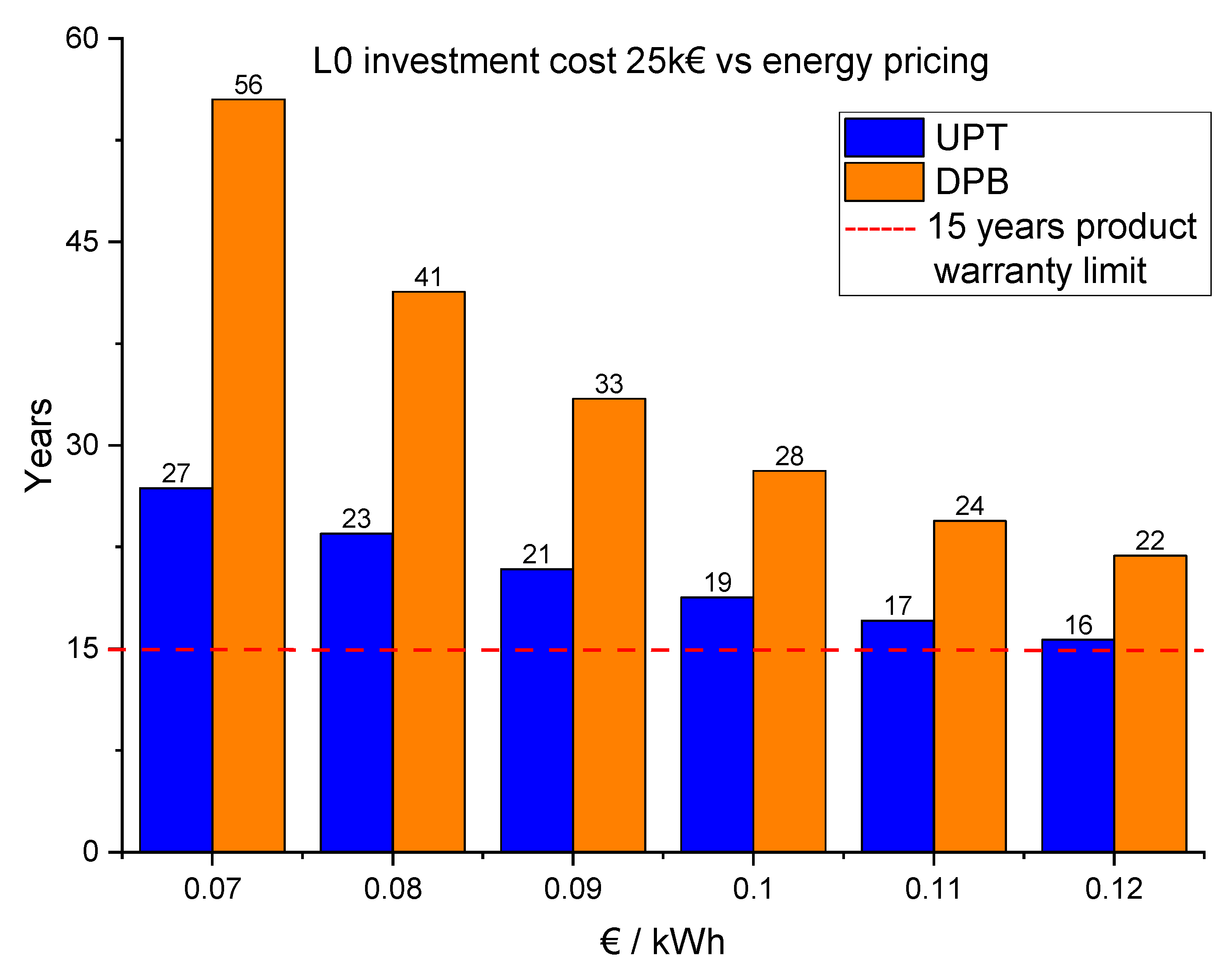
The payback period calculated in the previous research [15] (LEF cost 152 €/m2 and in total 25 k€) was around 30 years, which was beyond the product warranty of 15 years. However, that calculation was based on a very low energy price, which was around 0.07–0.08 €/kWh. The recent pricing in Sweden was an average of 0.12 €/kWh, which made the UPT around 16 years (Figure 23). As the energy crisis is looming in Europe, the prices in Sweden will follow suit, and these investments will have a much better payback time for the scenarios. For the same investment, using DPB with the internal rate of return (D%) of 3%, it would take about 22 years to pay off the investment. In some research [34], the D% used is as high as 5%, which would result in a DPB of 31 years. The UPT and DPB of L0 were revisited, given the understanding that energy prices have been rising steadily during the year 2022 in Sweden, as well as across Europe. The forecasted prices are way beyond what was reported in [15], and therefore, the prices chosen for the feasibility study did not exceed 0.12 €/kWh. The results were still beyond the 15 years warranty that the manufacturing company gave as the UPT of 16 years and DPB of 22 years at the price of 0.12 €/kWh. Now that the prices in Sweden as well as across Europe have risen dramatically due to the instability of the energy markets, both of the payback periods should decrease.
3.7. Economic Feasibility—Investment in GHP
The energy savings in CB0 and CL0 with B0 were found to be 165.1 and 170 MWh/year, respectively. These savings were converted into monetary savings, listed in Table 8, that would consequently be used as CFs in the UPT and DPB analysis. The energy savings of GHP (CB0 and CL0) were more than ten times the value of L0. If the total price of GHP unit(s) with a COP of 4.0 or higher (to cover the heating load of the building) were around 60 k€ with an installation and maintenance cost of 20 k€ for 15 years, the total price would become 80 k€ for CB0. For CL0, the price of L0 as 25 k€ was added to the sum, which led to a total of 105 k€. An extended energy price range of 0.07–0.18 €/kWh and its effects on the savings can be seen in Table 8.
The UPT and DPB for both CB0 and CL0 were calculated in Figure 24. Three different D% were used: 3, 8, and 11%. The investment of a GHP of CB0 would barely make it through the 15 years mark at D% of 11%. CL0 had longer UPT and DPB at the beginning, but then it became relatively close, as the energy price started to increase. The energy savings of both CB0 and CL0 were found to be around 20 k€ per year at the energy price of 0.12 €/kWh with a UPT and DPB that were much less than that of the LEF case at D% of 3 and 5%. In fact, the energy savings each year with GHP in both cases were about 80% of the investment and installation costs of LEF alone. This result, in combination with the reduced energy usage and emissions, makes GHPs a very attractive retrofitting measure that fulfills the visions of an increased BEP while sustaining an acceptable thermal comfort level.
4. Conclusions
This research evaluated the possibility of implementing energy saving measures by changing various parameters in a building as well as an energy sensitivity analysis based on geographical locations that involved different climate regions. This was done for a historical building, the City Hall (Rådhuset), in Gävle, which is used as an office building for the municipality. The various parameters evaluated were facade orientation, window shadings, LEF, different geographical locations, and alternative energy supply. Another goal would be to examine the economic feasibility of the investment in the newly added parameters if the parameters resulted in energy savings. Comparisons between B cases showed the largest difference between B0, the base case, and B4, which was the case with ES that was sun-controlled. This difference was an increase of 5.2 kWh/m2∙year. In evaluating B0, when focusing on geographical locations, the results demonstrated that the building required much more energy for heating in Gävle compared to the locations that were in warmer climate regions such as Beirut and Jakarta, where more cooling was required.
A reduction of SHGs was observed when comparing the cases without shading, B0–B1 to B2–B4. The largest reduction of SHG was made by B4 which was ES with sun-controlled configuration. It was also demonstrated that SHG for B0 was affected significantly by the location of the city and its closeness to the equator. Jakarta and Beirut had the highest level of SHG, while Gävle had the lowest. The total SHG for Jakarta was 48.1 kWh/m2∙year, compared to Gävle, which was 34.9 kWh/m2∙year. B4 had the best overall thermal comfort level as well as higher SDEI level amongst B0–B4. The PPD obtained for B4 was 36% lower than for B0.
When evaluating the energy usage for L cases (L0–L4) and looking specifically into L0, the largest difference between L0 and other L configurations was L4, which was similar to B0–B4. A similar development was also witnessed when assessing L0 cases in different geographical locations compared to their B0 counterparts. Once again, the evaluation of SHG, both locally with L0–L4 and with different geographical locations for L0, follows the same pattern as their B counterparts, but with a lower level of SHG, owing to LEF. In terms of the thermal comfort evaluation for L0–L4, the results indicated that L4 had the best overall thermal comfort level, as well as the highest level of SDEI compared to other L cases.
The results from investigating the best thermal comfort configuration for each location demonstrated that the building was not equipped with any cooling unit beside the HVAC that was able to cool down the supply air to 16 °C. However, this did not provide enough cooling for locations such as Beirut and Jakarta.
The CO2 emissions of B0 compared to all other B and L configurations illustrated that only B4 and B2 had higher emission levels than B0, and all other cases had lower emissions, with L1 having the lowest emission. The difference between B0 and L1 was 731 kg CO2 eq/year.
The impact of installing a GHP for B0 (CB0) and L0 (CL0) was examined, which indicated that there is a large reduction of the energy usage between B0 and CB0 by 57.5%, a reduction of the CO2 emissions by 35.4% (when using the Swedish average), and an increase of SDEI by 137.9%. Comparing B0 and CL0, the reductions of the energy usage and the CO2 emissions (when using the Swedish average) were 59.2% and 38.0%, respectively, while the increase of SDEI was 153.6%.
The economic feasibility of investing in LEF was calculated to 16 years when using the UPT method, and 22 years when utilizing the DPB method (D% = 3%), with the energy price of 0.12 €/kWh. The economic feasibility of investing in GHP for B0 (CB0) was calculated to 4.04 years when using the UPT method, and 4.36 years when applying the DPB method (D% = 3%), with the energy price of 0.12 €/kWh. Investing in GHP for L0 (CL0) was calculated to 5.2 years when using the UPT method, and 5.7 years when using the DPB method (D% = 3%), with the energy price of 0.12 €/kWh.
Lessons learned from this study were that one building code does not fit all, meaning that different locations require unique building specifications to ensure the comfort of occupants and to reduce the energy usage. When planning for a retrofit of old buildings, or any structures, it is important to investigate the portion of energy wasted in relation to energy consumed i.e., bought, so that correct measures and investments are prioritized instead of marginal ones. The building sector is facing drastic and dire times with energy prices on the rise.
It is worth mentioning some limitations as well. The model did not include any cooling systems that are required for hot climate regions, and this would have changed the outcome of the results. One possibility to expand this research would be to evaluate the installation of a photovoltaic system on the roof of the building, which could generate free electricity for the building.
Author Contributions
A.A.: Writing—Original Draft, Software, Conceptualization, Methodology, Visualization, Resources; A.B.: Formal analysis, Writing—Review and Editing; K.E.T.: Writing—Original Draft, Formal analysis, Visualization. All authors have read and agreed to the published version of the manuscript.
Funding
This research received no external funding.
Institutional Review Board Statement
Not applicable.
Informed Consent Statement
Not applicable.
Data Availability Statement
The data presented in this study are shown in the paper.
Acknowledgments
University of Gävle’s laboratory and technical staff for providing assistance with measuring equipment.
Conflicts of Interest
The authors declare no conflict of interest.
Nomenclature
| ACH | old building with very high ceiling |
| BEP | building energy performance |
| BPS | building performance simulation software |
| CF | cash flow |
| COP | coefficient of performance |
| DH | district heating |
| DPB | discounted payback time |
| D% | discount rate |
| ES | external shading |
| GHGs | greenhouse gases |
| GHP | geothermal heat pump |
| HVAC | heating, ventilation, and air conditioning |
| IS | internal shading |
| LEF | low energy film |
| NPV | net present value |
| PPD | percentage of total occupant hours with thermal dissatisfaction [%] |
| SDEI | satisfaction per delivered energy index [1/(kWh/m2∙year)] |
| SHG | solar heat gain |
| UPT | undiscounted payback time |
| WWR | window to wall ratio |
References
- Campagna, L.M.; Fiorito, F. On the Impact of Climate Change on Building Energy Consumptions: A Meta-Analysis. Energies 2022, 15, 354. [Google Scholar] [CrossRef]
- Barbir, F.; Veziroǧlu, T.N.; Plass, H.J. Environmental Damage Due to Fossil Fuels Use. Int. J. Hydrog. Energy 1990, 15, 739–749. [Google Scholar] [CrossRef]
- Pörtner, H.O.; Roberts, D.C.; Adams, H.; Adler, C.; Aldunce, P.; Ali, E.; Begum, R.A.; Betts, R.; Kerr, R.B.; Biesbroek, R.; et al. Climate Change 2022: Impacts, Adaptation and Vulnerability. IPCC Sixth Assess. Rep. 2022. [Google Scholar] [CrossRef]
- Zhai, Z.J.; Helman, J.M. Implications of Climate Changes to Building Energy and Design. Sustain. Cities Soc. 2019, 44, 511–519. [Google Scholar] [CrossRef]
- Sharma, S.K.; Mohapatra, S.; Sharma, R.C.; Alturjman, S.; Altrjman, C.; Mostarda, L.; Stephan, T. Retrofitting Existing Buildings to Improve Energy Performance. Sustainability 2022, 14, 666. [Google Scholar] [CrossRef]
- Fosas, D.; Coley, D.A.; Natarajan, S.; Herrera, M.; Fosas de Pando, M.; Ramallo-Gonzalez, A. Mitigation versus Adaptation: Does Insulating Dwellings Increase Overheating Risk? Build. Environ. 2018, 143, 740–759. [Google Scholar] [CrossRef]
- Fitton, R.; Swan, W.; Hughes, T.; Benjaber, M. The thermal performance of window coverings in a whole house test facility with single-glazed sash windows. Energy Effic. 2017, 10, 1419–1431. [Google Scholar] [CrossRef] [Green Version]
- Mohammed, A.; Tariq, M.A.U.R.; Ng, A.W.M.; Zaheer, Z.; Sadeq, S.; Mohammed, M.; Mehdizadeh-Rad, H. Reducing the Cooling Loads of Buildings Using Shading Devices: A Case Study in Darwin. Sustainability 2022, 14, 3775. [Google Scholar] [CrossRef]
- Morelli, M.; Rønby, L.; Mikkelsen, S.E.; Minzari, M.G.; Kildemoes, T.; Tommerup, H.M. Energy Retrofitting of a Typical Old Danish Multi-Family Building to a “Nearly-Zero” Energy Building Based on Experiences from a Test Apartment. Energy Build. 2012, 54, 395–406. [Google Scholar] [CrossRef]
- Harrestrup, M.; Svendsen, S. Full-Scale Test of an Old Heritage Multi-Storey Building Undergoing Energy Retrofitting with Focus on Internal Insulation and Moisture. Build. Environ. 2015, 85, 123–133. [Google Scholar] [CrossRef]
- Curto, D.; Franzitta, V.; Guercio, A.; Panno, D. Energy Retrofit. A Case Study—Santi Romano Dormitory on the Palermo University. Sustainability 2021, 13, 13524. [Google Scholar] [CrossRef]
- Cho, H.M.; Yun, B.Y.; Kim, Y.U.; Yuk, H.; Kim, S. Integrated Retrofit Solutions for Improving the Energy Performance of Historic Buildings through Energy Technology Suitability Analyses: Retrofit Plan of Wooden Truss and Masonry Composite Structure in Korea in the 1920s. Renew. Sustain. Energy Rev. 2022, 168, 112800. [Google Scholar] [CrossRef]
- Esteghamati, M.Z.; Sharifnia, H.; Ton, D.; Asiatico, P.; Reichard, G.; Flint, M.M. Sustainable Early Design Exploration of Mid-Rise Office Buildings with Different Subsystems Using Comparative Life Cycle Assessment. J. Build. Eng. 2022, 48, 104004. [Google Scholar] [CrossRef]
- Angrisano, M.; Fabbrocino, F.; Iodice, P.; Girard, L.F.; Ruello, M.L.; Mobili, A. The Evaluation of Historic Building Energy Retrofit Projects through the Life Cycle Assessment. Appl. Sci. 2021, 11, 7145. [Google Scholar] [CrossRef]
- Moghaddam, S.A.; Mattsson, M.; Ameen, A.; Akander, J.; Gameiro Da Silva, M.; Simões, N. Low-Emissivity Window Films as an Energy Retrofit Option for a Historical Stone Building in Cold Climate. Energies 2021, 14, 7584. [Google Scholar] [CrossRef]
- Woloszyn, M.; Rode, C. Tools for Performance Simulation of Heat, Air and Moisture Conditions of Whole Buildings. In Building Simulation; Springer: Berlin/Heidelberg, Germany, 2008; Volume 1, pp. 5–24. [Google Scholar]
- Ahmed, K.; Carlier, M.; Feldmann, C.; Kurnitski, J. A New Method for Contrasting Energy Performance and Near-Zero Energy Building Requirements in Different Climates and Countries. Energies 2018, 11, 1334. [Google Scholar] [CrossRef] [Green Version]
- Pieskä, H.; PLoSkić, A.; Wang, Q. Design Requirements for Condensation-Free Operation of High-Temperature Cooling Systems in Mediterranean Climate. Build. Environ. 2020, 185, 107273. [Google Scholar] [CrossRef]
- Kabanshi, A.; Ameen, A.; Hayati, A.; Yang, B. Cooling energy simulation and analysis of an intermittent ventilation strategy under different climates. Energy 2018, 156, 84–94. [Google Scholar] [CrossRef] [Green Version]
- Bakhtiari, H.; Akander, J.; Cehlin, M.; Hayati, A. On the Performance of Night Ventilation in a Historic Office Building in Nordic Climate. Energies 2020, 13, 4159. [Google Scholar] [CrossRef]
- Soleimani-Mohseni, M.; Nair, G.; Hasselrot, R. Energy Simulation for a High-Rise Building Using IDA ICE: Investigations in Different Climates. In Building Simulation; Springer: Berlin/Heidelberg, Germany, 2016; Volume 9, pp. 629–640. [Google Scholar]
- Hoffmann, T. SunCalc: Sun Position and Sunlight Phases Calculator. Available online: https://www.suncalc.org/ (accessed on 3 September 2022).
- Atzeri, A.; Cappelletti, F.; Gasparella, A. Internal Versus External Shading Devices Performance in Office Buildings. Energy Procedia 2014, 45, 463–472. [Google Scholar] [CrossRef]
- Hens, H.S.L. Building Physics-Heat, Air and Moisture: Fundamentals and Engineering Methods with Examples and Exercises; John Wiley & Sons: New York, NY, USA, 2017. [Google Scholar]
- Moreno, B.; Gonzalo, F.D.A.; Fernandez, J.A.; Lauret, B.; Hernandez, J.A. A Building energy simulation methodology to validate energy balance and comfort in zero energy buildings. J. Energy Syst. 2019, 3, 168–182. [Google Scholar] [CrossRef]
- Tzempelikos, A.; Athienitis, A.K. The Impact of Shading Design and Control on Building Cooling and Lighting Demand. Sol. Energy 2007, 81, 369–382. [Google Scholar] [CrossRef]
- Heydari, A.; Sadati, S.E.; Gharib, M.R. Effects of Different Window Configurations on Energy Consumption in Building: Optimization and Economic Analysis. J. Build. Eng. 2021, 35, 102099. [Google Scholar] [CrossRef]
- Vanek, F.M.; Albright, L.D.; Angenent, L.T. Energy Systems Engineering: Evaluation and Implementation; McGraw-Hill Education: New York, NY, USA, 2016. [Google Scholar]
- Rezaie, B.; Rosen, M.A. District Heating and Cooling: Review of Technology and Potential Enhancements. Appl. Energy 2012, 93, 2–10. [Google Scholar] [CrossRef]
- Rydegran, E. Fjärrvärmens Minskade Koldioxidutsläpp. Available online: https://www.energiforetagen.se/statistik/fjarrvarmestatistik/fjarrvarmens-koldioxidutslapp/ (accessed on 31 August 2022).
- Gävle Energi AB Gävle Energi-Productionmix. Available online: https://www.gavleenergi.se/om-oss/miljo-och-hallbarhet/fjarrvarme/ (accessed on 3 September 2022).
- Sandgren, A.; Nilsson, J. Emissionsfaktor För Nordisk Elmix Med Hänsyn till Import Och Export. Utredning Av Lämplig Systemgräns För Elmix Samt Beräkning Av Det Nordiska Elsystemets Klimatpåverkan. Norrköping. Nat. 2021. Available online: http://urn.kb.se/resolve?urn=urn%3Anbn%3Ase%3Anaturvardsverket%3Adiva-8809 (accessed on 26 August 2022).
- ANSI/ASHRAE Standard 55-2017; American Society of Heating and Refrigerating and Air-Conditioning Engineers Thermal Environmental Conditions for Human Occupancy. American National Standard: New York, NY, USA, 2017.
- Arnaoutakis, G.E.; Katsaprakakis, D.A.; Christakis, D.G. Dynamic Modeling of Combined Concentrating Solar Tower and Parabolic Trough for Increased Day-to-Day Performance. Appl. Energy 2022, 323, 119450. [Google Scholar] [CrossRef]
Figure 1.
Studied building; (a) plan of first floor, (b) southeast side of building [15].
Figure 1.
Studied building; (a) plan of first floor, (b) southeast side of building [15].

Figure 2.
Side view of southwest part of modeled building.

Figure 3.
Schedule for occupants, lighting, and equipment.

Figure 4.
Distribution system losses in model as well as hot water usage.

Figure 5.
Solar angles in various locations: (A) Gävle, (B) Sapporo, (C) Beirut, and (D) Jakarta [22].
Figure 5.
Solar angles in various locations: (A) Gävle, (B) Sapporo, (C) Beirut, and (D) Jakarta [22].

Figure 6.
Details of lightly woven curtains used for internal shading.

Figure 7.
Used ESs; temperature-controlled on the left and sun-controlled on the right.

Figure 8.
Breakdown of building’s annual energy usage for B0.

Figure 9.
Gävle—Delivered energy profile for B0–B4.

Figure 10.
Comparison between energy usage for B0 in different locations.

Figure 11.
SHG for Gävle under effect of different parameters.

Figure 12.
SHG for B0 in different locations.

Figure 13.
Thermal comfort main indicators as well as SDEIs for B0–B4 in Gävle.

Figure 14.
Breakdown of building’s annual energy usage for L0.

Figure 15.
Gävle—Delivered energy profile L0–L4.

Figure 16.
Comparison between energy usage for L0 in different locations.

Figure 17.
SHGs for Gävle under effect of L parameters including LEF windows.

Figure 18.
SHGs for L0 in different locations.

Figure 19.
Thermal comfort main indicators as well as SDEIs for L0–L4 in Gävle.

Figure 20.
Best possible thermal comfort configuration for each location.

Figure 21.
Difference between B0 and other configurations based on emission levels.

Figure 22.
Collective results for B0, L0, and C-cases.

Figure 23.
Different payback times: UPT and DPB (D% = 3%) of LEF investment.

Figure 24.
UPT and DPB with D% (3%, 8%, and 11%) for CB0 and CL0.


Table 1.
Thermal transmittance of building’s structural components.
| Structural Component | U-Value (W/(m2·K)) |
|---|---|
| External walls | 0.81 |
| Internal walls | 1.16 |
| Internal floors | 2.90 |
| External floors | 0.37 |
| Roof | 0.23 |
| Basement wall toward ground | 3.30 |
| Heated floor area: 1480 m2 Envelope area: 1910 m2 WWR: 11.7% | |
Table 2.
Linear heat loss coefficient of thermal bridges (W/(K·m)) for different types of joints in building.
Table 2.
Linear heat loss coefficient of thermal bridges (W/(K·m)) for different types of joints in building.
| Type of Joint | External Wall/Internal Slab | External Wall/Internal Wall | External Wall/External Wall | External Window Perimeter |
|---|---|---|---|---|
| Thermal bridges (W/(K·m)) | 0.58 | 0.23 | 0.25 | 0.05 |
Table 3.
Detailed properties of window.
| Type | U-Value (W/(m2·K)) | g-Value | Transmitted Visible Light |
|---|---|---|---|
| Double-Pane Window | 2.30 | 0.76 | 0.81 |
Table 4.
Internal gains in building.
| Type | Total | W |
|---|---|---|
| Occupants | 59 | 90 W |
| Lights | 450 | 24 W |
| Equipment | 59 | 125 W |
Table 5.
Evaluated locations (cities and countries), climate type, and climate file source.
| Location | Coordinates | Climate (M, P, T) | Climate File Source |
|---|---|---|---|
| Gävle Sweden | 60.6749° N 17.1413° E | Dfc (Snow, F. humidity, C. Summer) | SMHI Sveby |
| Sapporo Japan | 43.0618° N 141.3545° E | Dfb (Snow, F. Humidity, W. Summer) | ASHRAE IWEC2 |
| Beirut Lebanon | 33.8938° N 35.5018° E | Csa (Warm temperature, Dry warm summer) | ASHRAE IWEC2 |
| Jakarta Indonesia | 6.2088° S 106.8456° E | Af-Am (Equatorial, F. humid/Monsoonal) | ASHRAE IWEC2 |
Table 6.
Window data when LEF was applied.
| Type | U-Value (W/(m2·K)) | g-Value | Transmitted Visible Light |
|---|---|---|---|
| Window with applied LEF | 1.55 | 0.51 | 0.66 |
Table 7.
Case configuration list for B, L, and C-cases.
| Model Pre-LEF | Model Post LEF | Models with GHP |
|---|---|---|
| B0: Base model (BM) | L0: B0 + LEF | CB0: GHP + B0 |
| B1: (BM) + 90° clockwise rotation | L1: B1 + LEF | CL0: GHP + L0 |
| B2: BM + IS + sun control | L2: B2 + LEF | |
| B3: BM + ES + temperature control | L3: B3 + LEF | |
| B4: BM + ES + sun control | L4: B4 + LEF |
Table 8.
Energy price per kWh and corresponding energy savings in Euro for CB0 and CL0.
| Energy Price (€/kWh) | CB0 | CL0 |
|---|---|---|
| 0.07 | € 11,556 | € 11,901 |
| 0.08 | € 13,206 | € 13,601 |
| 0.09 | € 14,857 | € 15,301 |
| 0.10 | € 16,508 | € 17,001 |
| 0.11 | € 18,159 | € 18,701 |
| 0.12 | € 19,810 | € 20,401 |
| 0.13 | € 21,461 | € 22,101 |
| 0.14 | € 23,111 | € 23,802 |
| 0.15 | € 24,762 | € 25,502 |
| 0.16 | € 26,413 | € 27,202 |
| 0.17 | € 28,064 | € 28,902 |
| 0.18 | € 29,715 | € 30,602 |
Publisher’s Note: MDPI stays neutral with regard to jurisdictional claims in published maps and institutional affiliations. |
© 2022 by the authors. Licensee MDPI, Basel, Switzerland. This article is an open access article distributed under the terms and conditions of the Creative Commons Attribution (CC BY) license (https://creativecommons.org/licenses/by/4.0/).
Share and Cite
MDPI and ACS Style
Ameen, A.; Bahrami, A.; El Tayara, K. Energy Performance Evaluation of Historical Building. Buildings 2022, 12, 1667. https://0-doi-org.brum.beds.ac.uk/10.3390/buildings12101667
AMA Style
Ameen A, Bahrami A, El Tayara K. Energy Performance Evaluation of Historical Building. Buildings. 2022; 12(10):1667. https://0-doi-org.brum.beds.ac.uk/10.3390/buildings12101667
Chicago/Turabian StyleAmeen, Arman, Alireza Bahrami, and Khaled El Tayara. 2022. "Energy Performance Evaluation of Historical Building" Buildings 12, no. 10: 1667. https://0-doi-org.brum.beds.ac.uk/10.3390/buildings12101667
Note that from the first issue of 2016, this journal uses article numbers instead of page numbers. See further details here.