Compressive Strength Prediction of High-Strength Concrete Using Long Short-Term Memory and Machine Learning Algorithms

Abstract

Compressive strength is an important mechanical property of high-strength concrete (HSC), but testing methods are usually uneconomical, time-consuming, and labor-intensive. To this end, in this paper, a long short-term memory (LSTM) model was proposed to predict the HSC compressive strength using 324 data sets with five input independent variables, namely water, cement, fine aggregate, coarse aggregate, and superplasticizer. The prediction results were compared with those of the conventional support vector regression (SVR) model using four metrics, root mean square error (RMSE), mean absolute error (MAE), mean absolute percentage error (MAPE), and correlation coefficient (R²). The results showed that the prediction accuracy and reliability of LSTM were higher with R² = 0.997, RMSE = 0.508, MAE = 0.08, and MAPE = 0.653 compared to the evaluation metrics R² = 0.973, RMSE = 1.595, MAE = 0.312, MAPE = 2.469 of the SVR model. The LSTM model is recommended for the pre-estimation of HSC compressive strength under a given mix ratio before the laboratory compression test. Additionally, the Shapley additive explanations (SHAP)-based approach was performed to analyze the relative importance and contribution of the input variables to the output compressive strength.

1. Introduction

Concrete has been widely used worldwide with its economic, monolithic, modular, and durable advantages. High-strength concrete (HSC), which is defined by the compressive strength of more than 40 MPa [1], was developed in the late 1950s and early 1960s in the field of cementitious materials. The American Concrete Institute (ACI) defines HSC as “concrete that meets specific performance and homogeneity requirements that cannot always be achieved through the use of conventional materials and conventional mixing, placing and curing procedures”. Nowadays, HSC has been widely used in large-span bridges, high-rise buildings, and piers due to its uniform high density, low impermeability, and high durability [2].

To better understand design methods and the performance of concrete structures under external loads, it is of great importance to study the mechanical properties of concrete. Among the wide variety of concrete properties, the most important property is the compressive strength, as it is directly related to the safety of the structure and is necessary to assess the performance of the structure throughout its life cycle. However, concrete is a non-homogeneous mixture of cement, sand, gravel, supplementary raw materials, and admixtures. These ingredients are randomly distributed in the concrete mix ratio. Many factors affect the compressive strength of concrete, including waste composition, particle size, water-cement ratio, and aggregate ratio. Therefore, it is quite difficult to accurately predict the concrete compressive strength in such a complex matrix. The currently accepted method is to determine the compressive load-bearing capacity of concrete by physical tests. Generally, cubic and cylindrical concrete specimens are prepared according to certain mix ratios and cured for a period of time, and then the compressive strength of concrete is measured by a compressive testing machine. This method has been standardized around the world and is widely used for laboratory and field testing, but it is inefficient, economical, and time-consuming. In fact, for any kind of concrete with expected strength, the reasonable design of the mix ratio needs many attempts and laboratory tests. Moreover, the design procedure for HSC concrete is more complex than that for normal strength concrete, requiring experience and more in-depth knowledge of the chemical and mechanical properties of the components, and usually, several batches of tests are required to obtain the concrete with the desired properties. Thus, time and cost can be saved if the compressive strength can be estimated early and accurately through calculations before implementing the compression tests.

Empirical regression methods seem to be more suitable for assessing the compressive load-carrying capacity of concrete than traditional experimental techniques. With the development of artificial intelligence, it is very common and convenient to estimate the compressive strength of concrete using machine learning methods. Actually, machine learning algorithms such as artificial neural networks (ANN), random forest (RF), support vector machine (SVM), and decision tree (DT) have been widely used for the prediction of compressive strength of concrete [3,4,5,6,7,8,9,10,11]. Hai et al. [12] proposed a deep neural network (DNN) to predict the compressive strength of rubber concrete, and achieved high accuracy and reliability with R = 0.9874. Abobakr et al. [13] developed an extreme learning machine (ELM) model to predict the compressive strength of high-strength concrete, and the results showed that the ELM method has good prediction accuracy and fast learning speed compared with the traditional back-propagation (BP) neural network. Muliauwan et al. [14] employed three intelligent algorithms, linear regression, ANN, and SVM on 1030 samples to investigate the most accurate mapping relationships between input and output in concrete mixtures, and results showed that these intelligent methods can predict compressive strength with high accuracy in predictive models without expensive laboratory experiments. Song et al. [15] utilized gene expression programming (GEP), ANN, DT, and bagging algorithms to predict the compressive strength of fly ash admixture concrete. The results indicated that the bagging algorithm outperformed the other three algorithms with the highest prediction correlation coefficient R² = 0.95. To explore the applicability of integrated learning models, Furqan et al. [16] employed machine intelligence algorithms with individual learners and integrated learners on 1030 data samples to predict the compressive strength of sustainable high-performance concrete prepared from waste materials. It was found that the use of integrated models in machine learning can improve the model performance compared to traditional machine learning algorithms. The results of these studies mentioned above demonstrated that machine learning showed good prediction performance in regression prediction of concrete strength. However, the algorithms in these studies are mostly traditional machine learning algorithms with limited predictive capability. To get better prediction performance, model tuning is needed to get the appropriate model parameters, but this task is also a considerable challenge. Compared with conventional machine learning algorithms, it may be a better choice to explore a deep learning model with better prediction performance.

With the application of deep learning in civil engineering, as a special form of recurrent neural network (RNN), long short-term memory network (LSTM) has been well performed in many regression problems which has the ability to learn long-term dependencies. Harun et al. [17] estimated the geopolymerization process of fly ash-based polymers using deep LSTM and machine learning models. The results showed that compared to the prediction accuracy of 98.83%, and 91.62% for SVR and K-nearest neighbor (KNN), the deep LSTM achieved a higher accuracy of 99.55%. Sarmad [18] used the LSTM model on 1030 samples to predict the compressive strength of high-performance concrete achieving high accuracy with R² = 0.98. Harun et al. [19] employed two deep learning methods, namely stacked autoencoders and LSTM network, to predict the compressive strength and ultrasonic pulse velocity of concrete containing silica fume at high temperatures, and the results showed that LSTM achieved better prediction results. Overall, the LSTM model has exhibited good performance in the prediction of mechanical properties of concrete, but there is still relatively little research in concrete strength prediction, and in-depth analysis and research are needed before further popularization and application. For this reason, this paper attempts to propose an LSTM-based prediction model to predict the HSC compressive strength and compare the prediction results with the conventional support vector regression (SVR) model.

2. Methodology

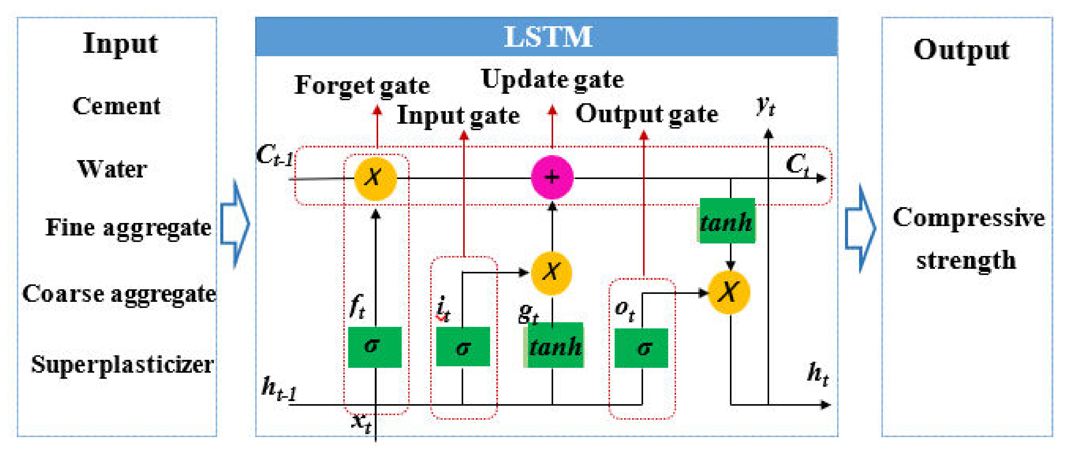
2.1. LSTM

The LSTM network was proposed by Hochreiter and Schmidhuber in 1997 [20], which aims to solve the problems of “gradient disappearance” and “gradient explosion” by introducing the gating function mechanism. As a powerful recurrent neural network model, LSTM can extract the long and short-term dependencies of time series, to achieve effective feature extraction of time-series data [21,22,23]. As shown in Figure 1, the LSTM includes the forget gate, input gate, update gate, and output gate in the principal structure. The main formulas of the LSTM structure are as follows [24,25]:

$$\left\{\begin{array}{l}{f}_t=\sigma (W_f(h_{t-1},x_t)+b_f)\\ i_t=\sigma (W_i(h_{t-1},x_t)+b_i)\\ g_t=\tanh (W_g(h_{t-1},x_t)+b_g)\\ c_t=f_t{c}_{t-1}+i_t{g}_t\\ o_t=\sigma (W_o(h_{t-1},x_t)+b_o)\\ h_t=o_t\tanh (c_t)\end{array}\right.$$

(1)

where f_t, i_t, g_t, and o_t determine the output values of the forget, input, update, and output gates, respectively; W_f, W_i, W_g, and W_o are weight vectors, b_f, b_i, b_g, and b_o are bias vectors; c_t and σ are memory cell and sigmoid activation functions, respectively.

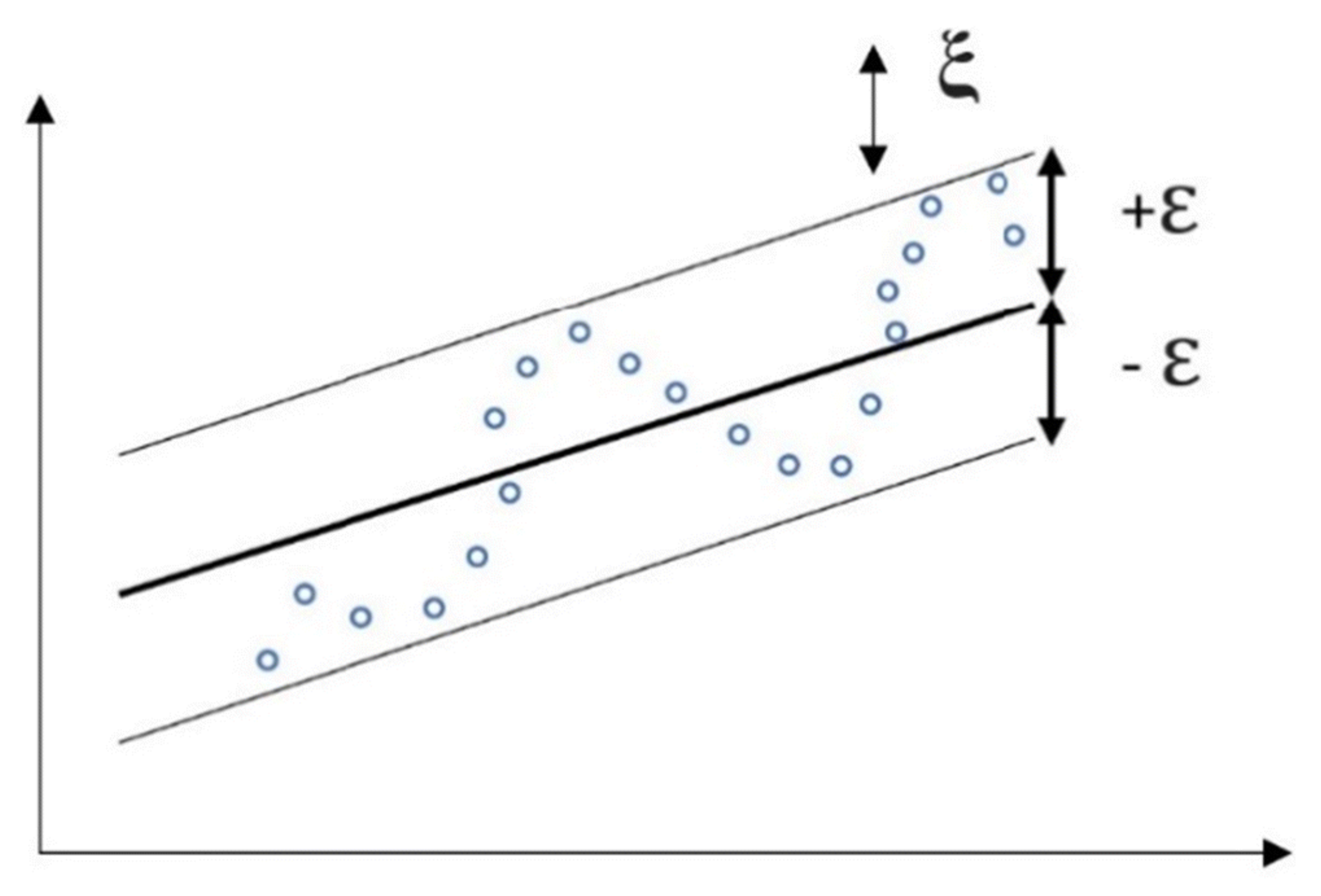
2.2. Support Vector Regression

Support vector regression (SVR) is an application of SVM in regression problems. Compared with ANN, SVM can handle nonlinear regression problems better and has the advantage of obtaining better global optimal solutions rather than local optimal solutions. Moreover, this model is accurate in prediction strength and easy to implement compared to other methods [26]. As shown in Figure 2, SVR adopts the concept of the ε-insensitive zone, in which a margin is defined to control the deviation of the prediction points. In linear SVR, the function f(x) is used as the solution of the problem [27]:

$$f(x)=w^{T}x+b$$

(2)

where w is the weight vector, x is the input vector, and b is the bias. For the nonlinear case, a kernel function $\varphi (x)$ can be used to map the data to a high-dimensional space with a nonlinear kernel.

$$f(x)=w^T\varphi (x)+b$$

(3)

The linear regression algorithm can be implemented by mapping the data to a higher dimensional feature space. The coefficients w and b can be determined by minimizing the following functions [28].

$$\left\{\begin{array}{l}\mathrm{Minimize} \frac{1}{2}{w}^T+C{\displaystyle \sum _{i=1}^n({\xi }_i+{\xi }_i^{*})}\\ y_i-w^T\varphi (x)-b\le \epsilon +{\xi }_i\\ w^T\varphi (x)+b-y_i\le \epsilon +{\xi }_i^{*}\\ {\xi }_i,{\xi }_i^{*}\ge 0\end{array}\right.$$

(4)

where n is the number of samples, C is the penalty parameter, and C is greater than 0. ${\xi }_i$ and ${\xi }_i^{*}$ are two slack variables. Considering that the Gaussian radial basis function is the most widely used, it is adopted as the kernel function in this paper. Its expression can be expressed as follows [29].

$$K(x_i,x)=\exp (-g{‖x_i-x‖}^2)$$

(5)

3. Materials and Dataset

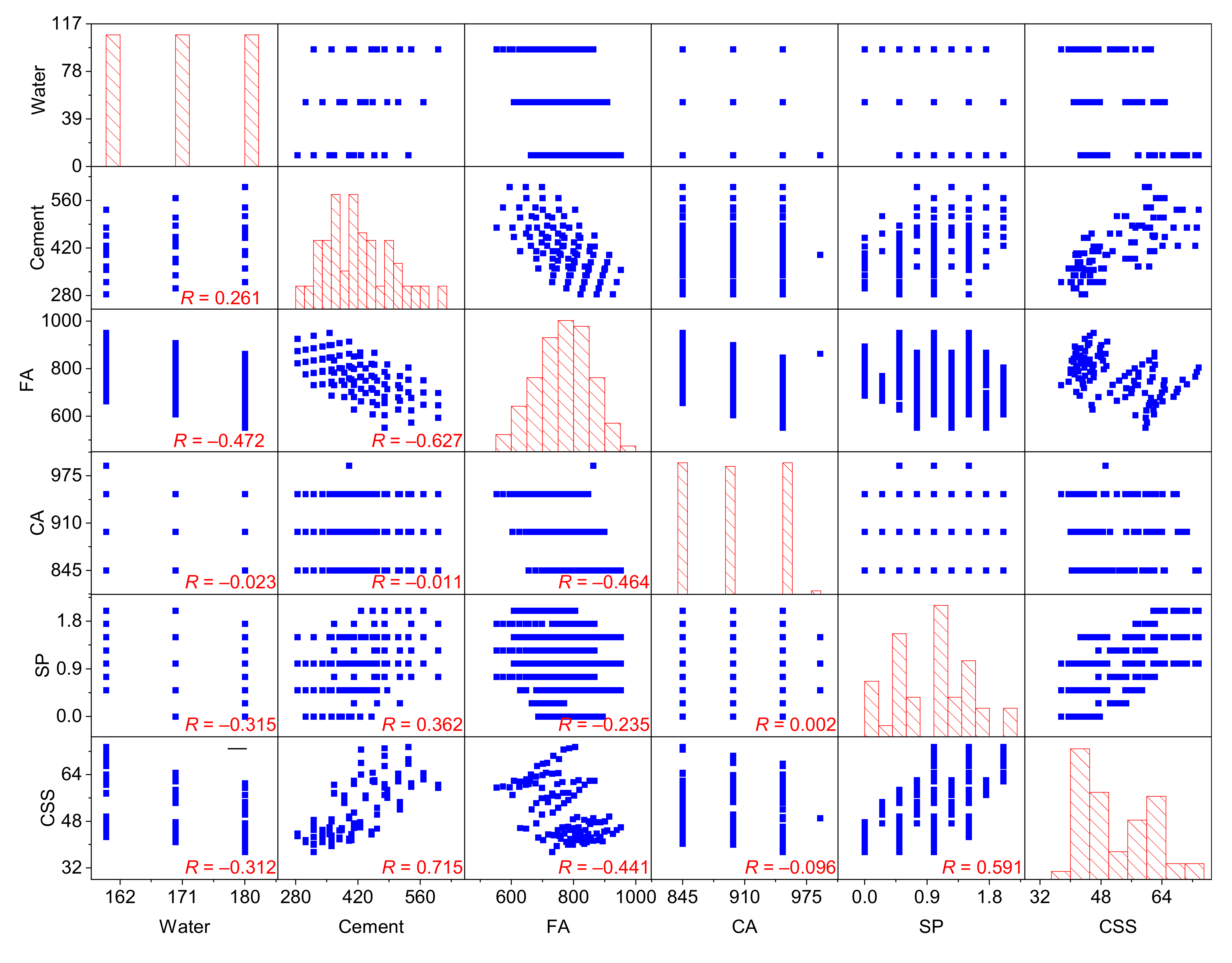
3.1. Dataset Description

The data set consists of 324 sets of samples collected from the literature [13], each containing 5 input variables and 1 output compressive strength. The input variables are water, cement, fine aggregate, coarse aggregate, and superplasticizer. For convenience, the abbreviations of all variables can be found in the Abbreviations. Figure 3 shows the distribution of these variables and the Pearson correlation coefficients between them. The linear correlation between the individual input variables and the output was found to be weak, indicating a complex nonlinear regression relationship between the five input variables and the compressive strength. About 80% of the samples were randomly selected and used for training, and the remaining 20% for testing. The statistical characteristics of these data sets are shown in

Table 1. Statistical characteristics of input and output parameters.

Variable		Water	Cement	Fine Aggregate	Coarse Aggregate	Superplasticizer	Compressive Strength
Abbreviation		Water	Cement	FA	CA	SP	CSS
Unit		kg/m3	kg/m3	kg/m3	kg/m3	kg/m3	MPa
Training set	max	180	600	951	989	2	73.6
	min	160	284	552	845	0	37.5
	average	168.02	410.76	712.05	902.76	0.80	51.98
	standard deviation	5.19	81.93	103.45	37.34	0.52	9.36
	kurtosis	−1.01	−1.01	−1.01	−1.01	−1.01	−1.01
	skewness	0.46	0.46	0.46	0.46	0.46	0.46
Test set	max	180	600	951	989	2	73.6
	min	160	284	552	845	0	37.5
	average	167.89	408.68	709.42	901.81	0.79	51.74
	standard deviation	5.38	84.99	107.31	38.73	0.54	9.71
	kurtosis	−1.05	−1.05	−1.05	−1.05	−1.05	−1.05
	skewness	0.40	0.40	0.40	0.40	0.40	0.40

.

3.2. Performance-Evaluation Methods

In general, when assessing the implementation of a prediction model, it is important to use various measures of evaluation metrics to assess the model’s effectiveness. In this paper, four metrics, root mean square error (RMSE), mean absolute error (MAE), mean absolute percentage error (MAPE), and correlation coefficient (R²), were used to analyze the predictive performance. These metrics are defined as follows [31]:

$$RMSE=\sqrt{\frac{1}{n}{\displaystyle \sum _{i=1}^n{(t-y)}^2}}$$

(6)

$$MAE=\frac{1}{n}{\displaystyle \sum _{i=1}^n(t-y)}$$

(7)

$$MAPE=\frac{1}{n}{\displaystyle \sum _{i=1}^n\left|\frac{t-y}{y}\right|}$$

(8)

$$R^2=\frac{{({\displaystyle \sum _{i=1}^n(t-\overline{t})}(y-\overline{y}))}^2}{{{\displaystyle \sum _{i=1}^n(t-\overline{t})}}^2{\displaystyle \sum _{i=1}^n{(y-\overline{y})}^2}}$$

(9)

where t is the experimental value, y is the predicted value, $\overline{t}$ is the mean value of t, $\overline{y}$ is the mean value of y.

4. Model Building and Training

4.1. Model Building

The LSTM model developed has five inputs and one output. The number of hidden units was 300, and fully connected layers were 100 [18]. For the SVR model with RBF kernel function, the parameters c and g have a great effect on the predictive performance. Usually, the SVR model requires some optimization algorithms to obtain the best combination of parameters, but this is not in the scope of this paper. For this reason, a basic SVR model was used in this paper. According to the reference [32], the two parameters c and g were set to 1 and 0.1, respectively.

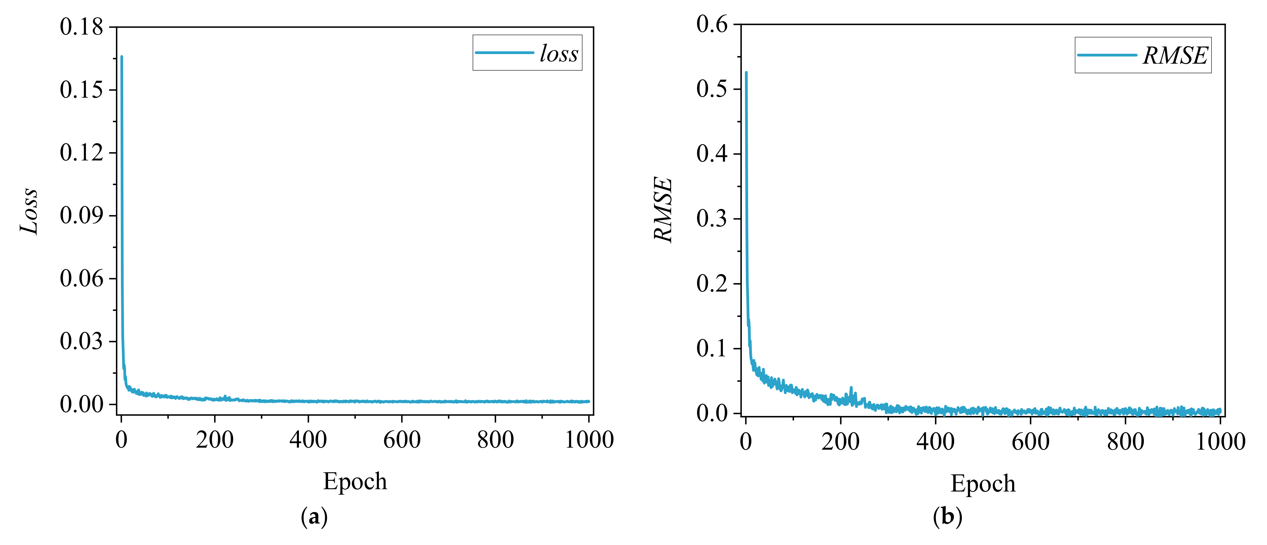
4.2. Model Training

First, the SVR model was performed to train the training set using ten-fold cross-validation. For comparison, the same training set was trained by the LSTM model. For the LSTM model, the training method was selected as the “adam”. Moreover, the mini-batch size was 64, the training epoch was 1000, and the gradient threshold used was 1. The initial learning rate was 0.001. The learning rate was used as a dropped factor 0.1 during the training with 250 epoch periods. The model was trained using MATLAB R2021a (The MathWorks Inc., Natick, MA, USA) on a laptop with Intel (R) Core (TM) i7 and 16 GB memory. Additionally, to speed up the training process, an NVIDIA™ GPU was used. The training process of the model is shown in Figure 4. It can be found that both RMSE and loss converged around 0 during the model training process, indicating that the model was well trained.

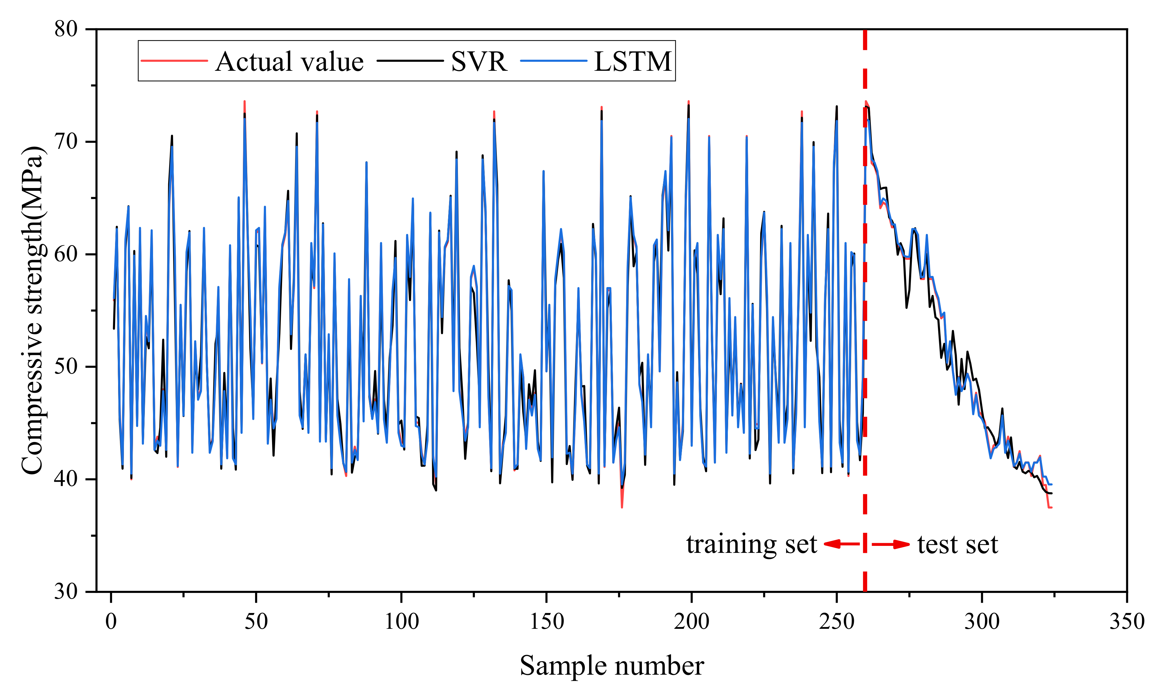
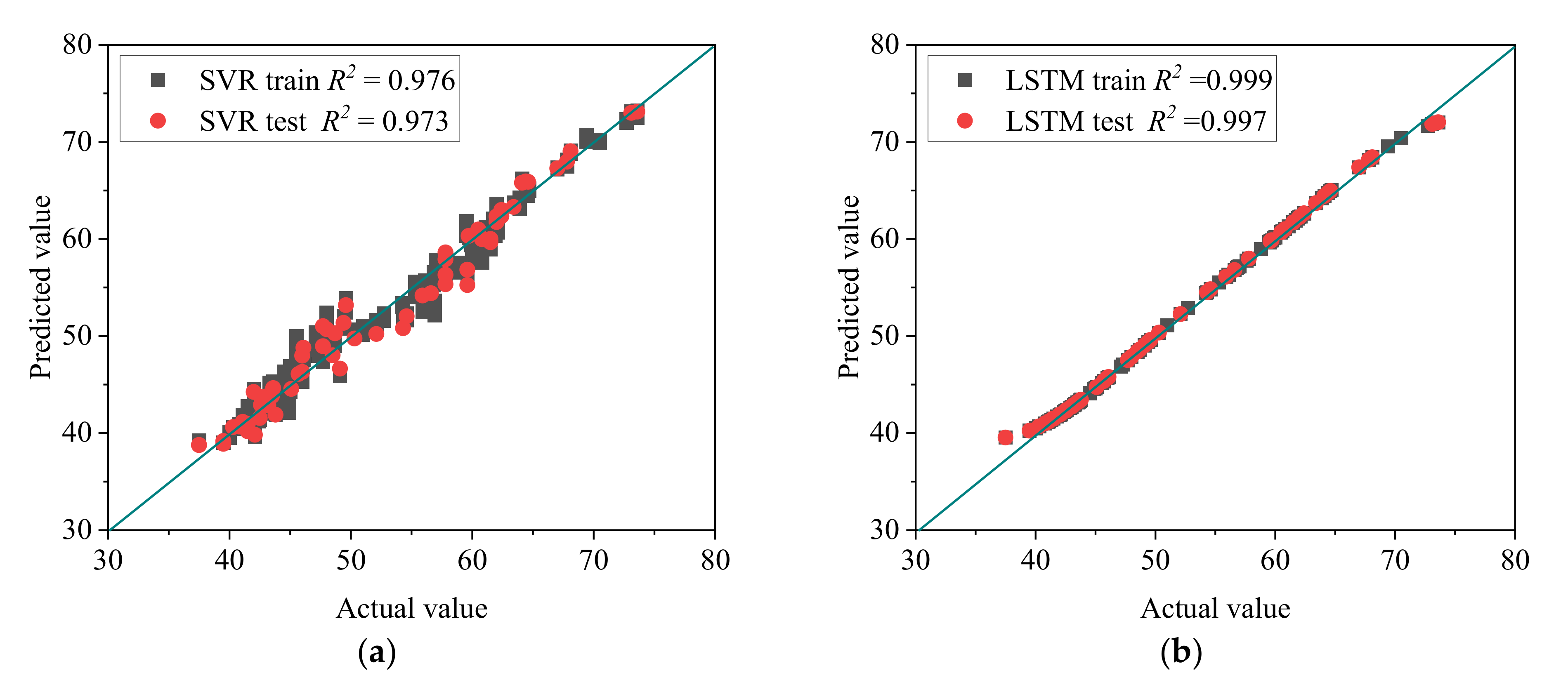
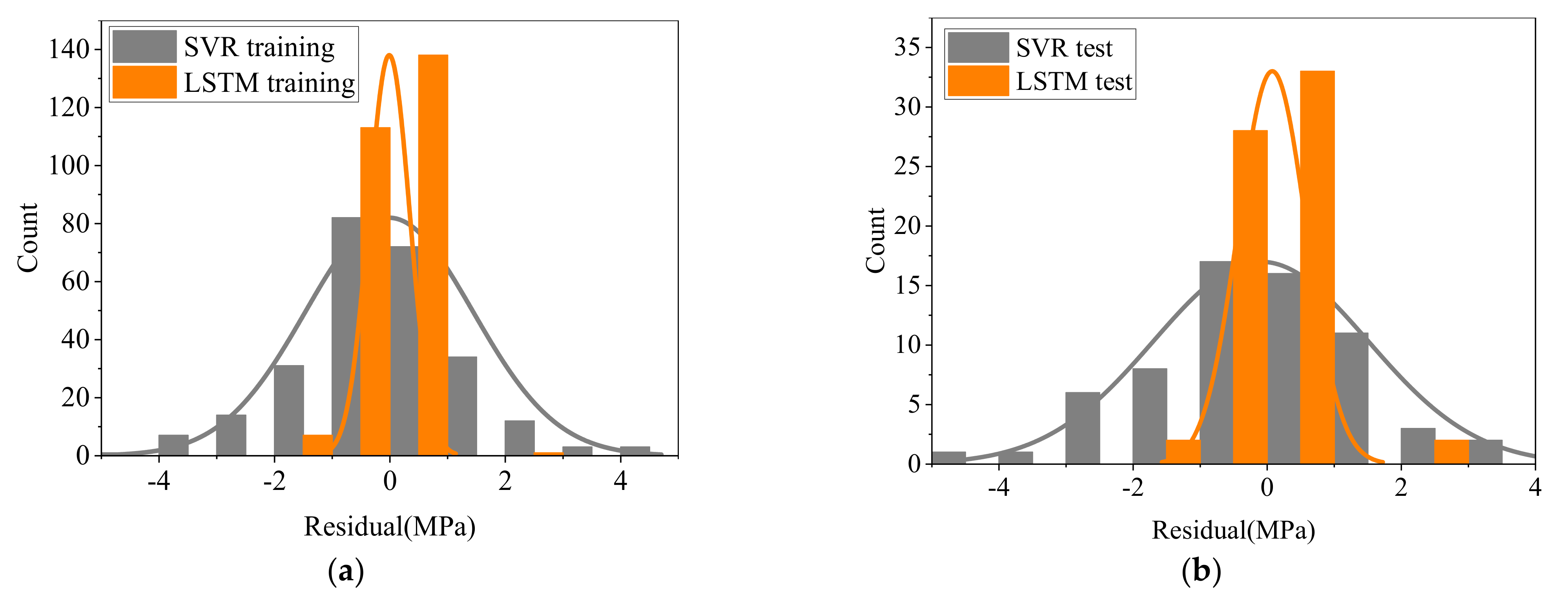
5. Comparison of Prediction Results

The predictions of the two models for the dataset are shown in Figure 5. It is obvious from the test set that the predicted values of the LSTM model match better with the actual values. For a more visual representation, the scatter plot of the prediction effect for each sample is shown in Figure 6. Compared with the SVR model, the scatter points in the LSTM model are closer to the diagonal, indicating that the model prediction accuracy is higher, which can also be seen from the fitted correlation coefficient between the predicted and actual values. Meanwhile, the residuals histogram of the statistical distribution is shown in Figure 7. The normal distribution curve of the residuals shows that the mean value of the predicted residuals of the LSTM model is closer to zero and the standard deviation is smaller.

The prediction output was statistically analyzed and the list of evaluation metrics is shown in

Table 2. Performance comparison of two models.

Model Type	Dataset	RMSE	MAE	MAPE(%)	R2
SVR	Training set	1.447	1.083	2.134	0.976
	Test set	1.595	0.312	2.469	0.973
LSTM	Training set	0.354	0.271	0.528	0.999
	Test set	0.508	0.080	0.653	0.997

. Compared with SVR, higher model prediction accuracy was obtained by the LSTM model with R² = 0.997, RMSE = 0.508, MAE = 0.08, and MAPE = 0.653, which could be recommended as a candidate for the compressive strength prediction tool of HSC. Moreover, these results further validate the ability of the LSTM model to capture the complex nonlinear relationship between the five input parameters and the compressive strength of the HSC.

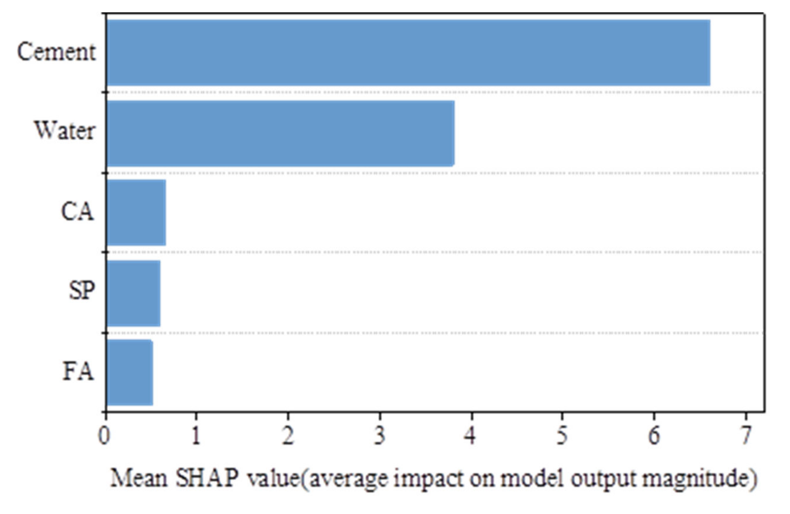
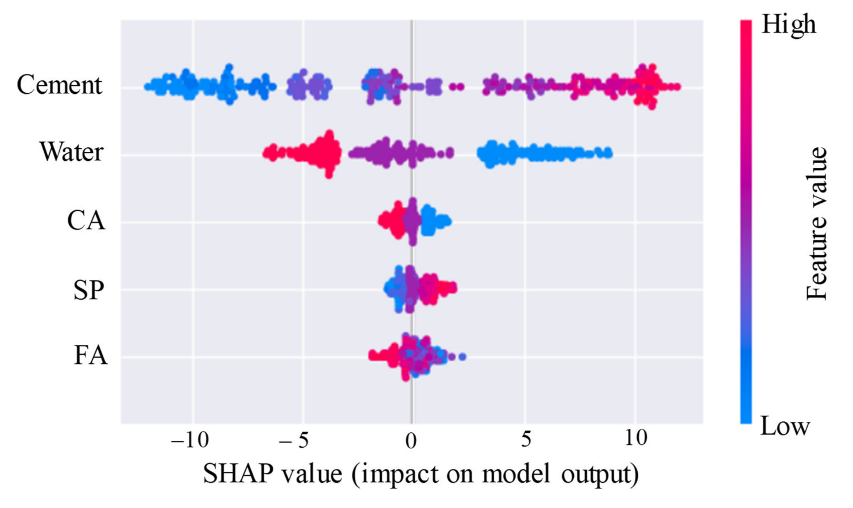
6. Importance Analysis of Input Variables on Output

The results of Section 4 show that given a mix ratio, a more accurate compressive strength estimate can be obtained based on the LSTM model. For HSC, if the pre-estimated compressive strength of the mix-design does not meet the designer’s expectation, then the content of each ingredient needs to be continuously adjusted to re-form a suitable mix-design. However, without knowing the effect and contribution of each input variable to the predicted output, these attempts are blind and require a lot of trial and error. For this reason, a Shapley additive explanations(SHAP)-based method was proposed to investigate the relative importance of each input variable to the output results and whether each variable contributes positively or negatively to the output results [33]. A detailed description of the SHAP approach can be seen in references [34,35].

As shown in Figure 8, the average SHAP values shown represent the relative importance of the input variables on the output. It can be clearly observed that among the five variables listed in this paper, cement has the greatest effect on HSC compressive strength, followed closely by water, coarse aggregate, superplasticizer, and fine aggregate. In addition, the summary plot used to elucidate the influence of the global characteristics of the input features is shown in Figure 9, where each point represents the Shapley value of a feature and a separate observation in the dataset. The position of each point on the x-axis represents the Shapley value for each factor, showing the effect of each factor on compressive strength, while the y-axis provides the order of importance of each factor. A high feature value for each sample in Figure 9 indicates that this input variable is positive for the output compressive strength. Conversely, the smaller the feature value, the more negative the input variable is on the output. It can be clearly observed that cement and superplasticizer are positive for the compressive strength and the compressive strength increases with the increase of their amount. On the contrary, water, coarse aggregate, and fine aggregate are negative for compressive strength, and an increase in the amount of these three ingredients leads to a decrease in the compressive strength of HSC.

The findings in this section can help designers and constructors understand the importance of each component in concrete to the output compressive strength and whether it is positive or negative to the output compressive strength. Moreover, it can help operators significantly reduce the time and cost of adjusting the amount of each component when preparing a mix ratio for the desired strength concrete.

7. Conclusions

In this paper, the LSTM model was employed to predict the HSC compressive strength, and the predicted results were compared with a conventional SVR model. The main conclusions are summarized as follows.

(1)

The LSTM model can capture the complex nonlinear relationship between the five input parameters and the compressive strength of HSC with R² exceeding 0.99 in both training and testing stages.

(2)

Compared with the conventional SVR model, the prediction capacity of the LSTM model is superior, which is recommended as an alternative method for the compressive strength prediction of HSC. The pre-estimate HSC compressive strength can be obtained prior to the implementation of laboratory compression tests using the LSTM model, which will greatly reduce the time and cost of laboratory compression tests.

(3)

Among the five input variables shown in this paper, cement and water are the two most sensitive and important variables for compressive strength.

(4)

Cement and superplasticizer are positive for compressive strength, the value of compressive strength increases with their increase, while water, coarse aggregate, and fine aggregate are negative for compressive strength, their increase will lead to the decrease of compressive strength of HSC.

References

- Henry, G.R. ACI Defines High-Performance Concrete. Concr. Int. 1999, 21, 56–57. [Google Scholar]
- Mbessa, M.; Péra, J. Durability of high-strength concrete in ammonium sulfate solution. Cem. Concr. Res. 2001, 31, 1227–1231. [Google Scholar] [CrossRef]
- Moradi, M.J.; Khaleghi, M.; Salimi, J.; Farhangi, V.; Ramezanianpour, A.M. Predicting the compressive strength of concrete containing metakaolin with different properties using ANN. Measurement 2021, 183, 109790. [Google Scholar] [CrossRef]
- Azimi-Pour, M.; Eskandari-Naddaf, H.; Pakzad, A. Linear and non-linear SVM prediction for fresh properties and compressive strength of high volume fly ash self-compacting concrete. Constr. Build. Mater. 2020, 230, 117021. [Google Scholar] [CrossRef]
- Nguyen-Sy, T.; Wakim, J.; To, Q.-D.; Vu, M.-N.; Nguyen, T.-D.; Nguyen, T.-T. Predicting the compressive strength of concrete from its compositions and age using the extreme gradient boosting method. Constr. Build. Mater. 2020, 260, 119757. [Google Scholar] [CrossRef]
- Han, Q.; Gui, C.; Xu, J.; Lacidogna, G. A generalized method to predict the compressive strength of high-performance concrete by improved random forest algorithm. Constr. Build. Mater. 2019, 226, 734–742. [Google Scholar] [CrossRef]
- Li, H.; Lin, J.; Lei, X.; Wei, T. Compressive strength prediction of basalt fiber reinforced concrete via random forest algorithm. Mater. Today Commun. 2022, 30, 103117. [Google Scholar] [CrossRef]
- Ahmad, A.; Ahmad, W.; Aslam, F.; Joyklad, P. Compressive strength prediction of fly ash-based geopolymer concrete via advanced machine learning techniques. Case Stud. Constr. Mater. 2022, 16, e00840. [Google Scholar] [CrossRef]
- Barkhordari, M.S.; Armaghani, D.J.; Mohammed, A.S.; Ulrikh, D.V. Data-Driven Compressive Strength Prediction of Fly Ash Concrete Using Ensemble Learner Algorithms. Buildings 2022, 12, 132. [Google Scholar] [CrossRef]
- Silva, F.A.N.; Delgado, J.M.P.Q.; Cavalcanti, R.S.; Azevedo, A.C.; Guimarães, A.S.; Lima, A.G.B. Use of Nondestructive Testing of Ultrasound and Artificial Neural Networks to Estimate Compressive Strength of Concrete. Buildings 2021, 11, 44. [Google Scholar] [CrossRef]
- Ahmad, A.; Chaiyasarn, K.; Farooq, F.; Ahmad, W.; Suparp, S.; Aslam, F. Compressive Strength Prediction via Gene Expression Programming (GEP) and Artificial Neural Network (ANN) for Concrete Containing RCA. Buildings 2021, 11, 324. [Google Scholar] [CrossRef]
- Ly, H.-B.; Nguyen, T.-A.; Thi Mai, H.-V.; Tran, V.Q. Development of deep neural network model to predict the compressive strength of rubber concrete. Constr. Build. Mater. 2021, 301, 124081. [Google Scholar] [CrossRef]
- Al-Shamiri, A.K.; Kim, J.H.; Yuan, T.-F.; Yoon, Y.S. Modeling the compressive strength of high-strength concrete: An extreme learning approach. Constr. Build. Mater. 2019, 208, 204–219. [Google Scholar] [CrossRef]
- Muliauwan, H.N.; Prayogo, D.; Gaby, G.; Harsono, K. Prediction of Concrete Compressive Strength Using Artificial Intelligence Methods. J. Phys. Conf. Ser. 2020, 1625, 012018. [Google Scholar] [CrossRef]
- Song, H.; Ahmad, A.; Farooq, F.; Ostrowski, K.A.; Maślak, M.; Czarnecki, S.; Aslam, F. Predicting the compressive strength of concrete with fly ash admixture using machine learning algorithms. Constr. Build. Mater. 2021, 308, 125021. [Google Scholar] [CrossRef]
- Farooq, F.; Ahmed, W.; Akbar, A.; Aslam, F.; Alyousef, R. Predictive modeling for sustainable high-performance concrete from industrial wastes: A comparison and optimization of models using ensemble learners. J. Clean. Prod. 2021, 292, 126032. [Google Scholar] [CrossRef]
- Tanyildizi, H. Predicting the geopolymerization process of fly ash-based geopolymer using deep long short-term memory and machine learning. Cem. Concr. Compos. 2021, 123, 104177. [Google Scholar] [CrossRef]
- Latif, S.D. Concrete compressive strength prediction modeling utilizing deep learning long short-term memory algorithm for a sustainable environment. Environ. Sci. Pollut. Res. 2021, 28, 30294–30302. [Google Scholar] [CrossRef]
- Tanyildizi, H.; Şengür, A.; Akbulut, Y.; Şahin, M. Deep learning model for estimating the mechanical properties of concrete containing silica fume exposed to high temperatures. Front. Struct. Civ. Eng. 2020, 14, 1316–1330. [Google Scholar] [CrossRef]
- Hochreiter, S.; Schmidhuber, J. Long Short-Term Memory. Neural Comput. 1997, 9, 1735–1780. [Google Scholar] [CrossRef]
- Greff, K.; Srivastava, R.K.; Koutník, J.; Steunebrink, B.R.; Schmidhuber, J. LSTM: A Search Space Odyssey. IEEE Trans. Neural Netw. Learn. Syst. 2017, 28, 2222–2232. [Google Scholar] [CrossRef] [Green Version]
- Shrestha, A.; Mahmood, A. Review of Deep Learning Algorithms and Architectures. IEEE Access 2019, 7, 53040–53065. [Google Scholar] [CrossRef]
- Wang, K.; Qi, X.; Liu, H. Photovoltaic power forecasting based LSTM-Convolutional Network. Energy 2019, 189, 116225. [Google Scholar] [CrossRef]
- Moradzadeh, A.; Teimourzadeh, H.; Mohammadi-Ivatloo, B.; Pourhossein, K. Hybrid CNN-LSTM approaches for identification of type and locations of transmission line faults. Int. J. Electr. Power Energy Syst. 2022, 135, 107563. [Google Scholar] [CrossRef]
- Moradzadeh, A.; Zakeri, S.; Shoaran, M.; Mohammadi-Ivatloo, B.; Mohammadi, F. Short-Term Load Forecasting of Microgrid via Hybrid Support Vector Regression and Long Short-Term Memory Algorithms. Sustainability 2020, 12, 7076. [Google Scholar] [CrossRef]
- Naderpour, H.; Rafiean, A.H.; Fakharian, P. Compressive strength prediction of environmentally friendly concrete using artificial neural networks. J. Build. Eng. 2018, 16, 213–219. [Google Scholar] [CrossRef]
- Wu, Y.; Li, S. Damage degree evaluation of masonry using optimized SVM-based acoustic emission monitoring and rate process theory. Measurement 2022, 190, 110729. [Google Scholar] [CrossRef]
- Jiang, W.; Xie, Y.; Li, W.; Wu, J.; Long, G. Prediction of the splitting tensile strength of the bonding interface by combining the support vector machine with the particle swarm optimization algorithm. Eng. Struct. 2021, 230, 111696. [Google Scholar] [CrossRef]
- Ahmad, M.; Kamiński, P.; Olczak, P.; Alam, M.; Iqbal, M.J.; Ahmad, F.; Sasui, S.; Khan, B.J. Development of Prediction Models for Shear Strength of Rockfill Material Using Machine Learning Techniques. Appl. Sci. 2021, 11, 6167. [Google Scholar] [CrossRef]
- Ray, S.; Haque, M.; Rahman, M.M.; Sakib, M.N.; Al Rakib, K. Experimental investigation and SVM-based prediction of compressive and splitting tensile strength of ceramic waste aggregate concrete. J. King Saud Univ.-Eng. Sci. 2021; in press. [Google Scholar] [CrossRef]
- Nguyen, M.S.T.; Kim, S.-E. A hybrid machine learning approach in prediction and uncertainty quantification of ultimate compressive strength of RCFST columns. Constr. Build. Mater. 2021, 302, 124208. [Google Scholar] [CrossRef]
- Ling, H.; Qian, C.; Kang, W.; Liang, C.; Chen, H. Combination of Support Vector Machine and K-Fold cross validation to predict compressive strength of concrete in marine environment. Constr. Build. Mater. 2019, 206, 355–363. [Google Scholar] [CrossRef]
- Chakraborty, D.; Awolusi, I.; Gutierrez, L. An explainable machine learning model to predict and elucidate the compressive behavior of high-performance concrete. Results Eng. 2021, 11, 100245. [Google Scholar] [CrossRef]
- Mangalathu, S.; Hwang, S.-H.; Jeon, J.-S. Failure mode and effects analysis of RC members based on machine-learning-based SHapley Additive exPlanations (SHAP) approach. Eng. Struct. 2020, 219, 110927. [Google Scholar] [CrossRef]
- Bakouregui, A.S.; Mohamed, H.M.; Yahia, A.; Benmokrane, B. Explainable extreme gradient boosting tree-based prediction of load-carrying capacity of FRP-RC columns. Eng. Struct. 2021, 245, 112836. [Google Scholar] [CrossRef]