Multiple Defects Inspection of Dam Spillway Surface Using Deep Learning and 3D Reconstruction Techniques

Abstract

After a lengthy period of scouring, the reinforced concrete surface of the dam spillway (i.e., drift spillways and flood discharge spillways) will suffer from deterioration and damage. Regular manual inspection is time-consuming and dangerous. This paper presents a robotic solution to detect automatically, count defect instance numbers, and reconstruct the surface of dam spillways by incorporating the deep learning method with a visual 3D reconstruction method. The lack of a real dam defect dataset and incomplete registration of minor defects on the 3D mesh model in fusion step are two challenges addressed in the paper. We created a multi-class semantic segmentation dataset of 1711 images (with resolutions of 848 × 480 and 1280 × 720 pixels) acquired by a wall-climbing robot, including cracks, erosion, spots, patched areas, and power safety cable. Then, the architecture of the U-net is modified with pixel-adaptive convolution (PAC) and conditional random field (CRF) to segment different scales of defects, trained, validated, and tested using this dataset. The reconstruction and recovery of minor defect instances in the flow surface and sidewall are facilitated using a keyframe back-projection method. By generating an instance adjacency matrix within the class, the intersection over union (IoU) of 3D voxels is calculated to fuse multiple instances. Our segmentation model achieves an average IoU of 60% for five defect class. For the surface model’s semantic recovery and instance statistics, our method achieves accurate statistics of patched area and erosion instances in an environment of 200 m${}^2$, and the average absolute error of the number of spots and cracks has reduced from the original 13.5 to 3.5.

1. Introduction

As the most important water conservancy project, a dam will cause significant loss of life and property if it fails. As of December 2011, there were 98,002 reservoirs in China, with a total storage capacity of over 930 billion m${}^3$. Between 1954 and 2006, 3498 dams failed due to dam quality and overtopping [1]. With the construction of the Three Gorges Dam, flood discharge facilities will need regular maintenance and overhaul [2]. The defects are categorized as follows, during the inspection process: the interior of the concrete, the surface, and the leaking. Operator visual inspection and recording are the primary way to monitor surface defects. Interior and leaking flaws are usually identified using a combination of physical methods such as drilling cores, acoustic computed tomography (CT) testing, and pressurized water testing. Detecting surface defects is easier to carry out, but the impact of interior and leaking defects on the structure is more serious. Since surface data is easier to obtain for computer vision, some prominent defect areas can be preliminarily judged. For this reason, the detection and statistics of surface defects can provide a reference for the subsequent detection of more severe interior and leaking defects. In recent years, computer vision approaches have gradually been applied to tasks such as surface flaw detection and overall dam reconstruction. Drones were employed in Khaloo’s [3] study to establish a general 3D model of the dam using the structure from motion (SFM) approach. Improving the resolution makes it possible to detect surface flaws down to the millimeter scale [4]. Khaloo uses space color hue to detect the relevant transformation of gravity dams [5], Angeli provides operators with a convenient interface for defect marking by constructing a dense point cloud on the dam’s surface [6]. Some researchers only built the overall point cloud model of the dam using images and set calibration facilities [7,8]. Image stitching can also be used for the downstream section of the dam, image reconstruction of the dam sidewalls, and the underwater section of the dam [9,10]. The dam’s flood discharge spillways and drift spillways are also the focus of the maintenance procedure, in comparison to the long-term monitoring of the dam, because they frequently experience scouring by water flow. Our previous work used the SLAM approach to reconstruct the sidewall of drift spillways with crack flaws [11]. Dam surface monitoring needs to realize defects’ segmentation, statistics, and reconstruction. There are two challenges in the application of the deep learning-based defect segmentation and truncated signed distance field(TSDF) fusion 3D reconstruction method: First, there is a lack of multi-defect dataset suitable for training of deep learning for dam surface inspection, and the simple deep learning network is difficult to distinguish defects classes that have large scale difference on the dam surface (e.g., small spot vs. large patched area). Second, the incomplete registration of sparse defect pixels in the TSDF fusion step affects the three-dimensional visualization and statistics count of different defects. The following is an overview of our contributions:

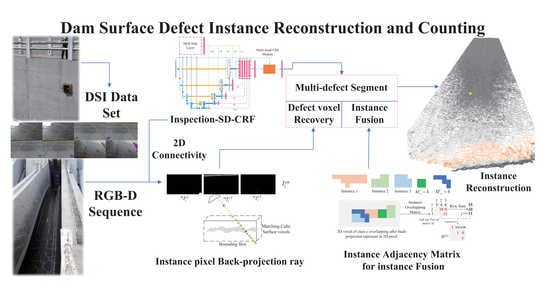
• We use the images collected by the wall-climbing robot to build the first pixel-level segmentation dataset of dam surface defects, including patched area, spot, erosion, crack, and spalling. Moreover, we propose a multi-level side-out structure with CRF layers optimization to improve the IoU of the model segmentation results for multiple classes.
• We solve the defects incomplete registration problem by proposing the class instance rays back-projection approach to re-register the disappeared defects pixels onto the surface 3D mesh model.
• We propose an instance adjacency matrix to fuse the same defect class instance by setting a 3D intersection over union threshold, which can facilitate the defect instance statistic problem.

The rest of the paper is organized as follows: Section 2 introduces related works. Section 3 introduces the wall-climbing robot’s image collection system and dataset. Section 4 and Section 5 describe PAC-based multi-level structure and keyframes back-projection-based defect instance voxel fusion. Section 6 presents the experimental results of defect segmentation, defect instance voxel recovery, and defect instance counting. Section 7 summarizes the paper and discusses further research.

2. Related Works

2.1. Concrete Surface Defect Detection Based on Deep Learning

Defect detection is a significant part of the inspection task. Deep learning-based methods have been applied to concrete tunnels, bridges, and buildings, not just dams. Some researchers use target detection for quick multi-defect localization and identification. Yeum et al. employs AlexNet to detect post-disaster collapse, spalling, building column, and façade damage [12]. Gao detects spalling, building column, shear damage, and other building defects using VGG combined with transfer learning [13]. Li et al. detects cracks and rebar exposure of concrete surface using Faster R-CNN [14]. Gao segment tunnel cracks and leaks using Faster R-CNN in conjunction with fully convolution network(FCN) [15]. Inspection-Net [16] is used to segment spalling and cracking within a tunnel. Hong investigates a more suitable loss function for Inspection-Net [11]. As an advanced crack and spalling segmentation network, Inspection-Net achieves the best recognition accuracy on the CSSC dataset. Still, on the proposed multi-defect dataset, it can only perform an average IoU of 51%. Our proposed improved model increases this indicator by 9%, and only increases the number of parameters by 75 Kb. Tang et al. propose a valuable definition of crack width that combines the macroscale and microscale characteristics of the backbone to obtain accurate and objective sample points for width description [17]. Zhang uses YOLO (you only look once network) in conjunction with FCN for fast crack, spalling, and rebar segmentation [18]. Azimi and Eslamlou et al. outline some defect detection and segmentation dataset [19], and Yang creates a semantic segmentation dataset that includes concrete surface spalling and cracks (CSSC) [16]. Li and Zhou provide a concrete multi-defect segmentation dataset [20]; however, the multi-class images in their dataset are insufficient, and most images were collected in a laboratory environment with a look-down camera, which is not favorable for complex work in practice. Spencer indicates that the deep learning model lacks the generalization ability to segment flaws on different types of surfaces such as concrete and asphalt [21]. Our research establishes the first multi-defect dataset specifically for concrete surface by combining CSSC dataset with the data we collect from spillway sidewalls, which will be discussed in Section 3.

2.2. 3D Reconstruction and Modeling

In addition to the defect detection based on 2D images, the inspection task of the dam surface also requires to determine the location of the defects in 3D space and obtain metric information such as the length, area, and the number of defects. Therefore, registering 2D semantic information into a 3D model is necessary. Most of the traditional methods use dense point cloud for 3D reconstruction. Izadi et al. uses the image pose and scale information to calculate the TSDF and combines the marching cube theory [22] to construct a surface mesh [23]. Poisson reconstruction method uses indicator function to make point clouds more smooth. SLAM++ [24] and TSDF++ [25] construct a 3D semantic model using the deep neural network to obtain semantic labels. Aiming at constructing a surface semantic model of concrete buildings, Jahanshahi uses the method of keyframes combined with SFM to reconstruct the 3D point cloud of defects on walls [26]. Yang uses TSDF to connect the semantic segmentation model and the CRF fusion method between keyframes to perform a 3D semantic reconstruction of the tunnel surface [27]. This mesh model is beneficial to the follow-up defect assessment and measurement. Our previous research uses ORB-SLAM2 [28] for localization and mapping and uses neural network for crack segmentation to construct a 3D model of dam surface. Insa-Iglesias uses SFM combined with virtual reality to realize a remote real-world monitoring method for tunnel assessment [29]. Tang et al. propose a four-ocular vision system for the three-dimensional (3D) reconstruction of large-scale concrete-filled steel tube(CFST) under complex testing conditions [30]. Most researches have not involve the study of defects counting. Due to the inaccuracy of depth measurement, the TSDF-based method in the dam surface semantic reconstruction mission sometimes may experience semantic information loss; we called it incomplete registration from 2D segmentation results to the 3D model. Section 4 presents keyframes back-projection and voxel IoU threshold approaches to realize complete instance registration and instance counting of different classes.

3. Robotic Visual Inspection System

We use a wall-climbing robot to collect visual image data from the Three Gorges Dam’ No. 3 drift spillway and No. 1 deep spillway. Figure 1 shows the field testing environment and the climbing robot.

3.1. Image Data Collection

As illustrated in Figure 1c,d, the robot uses negative pressure adsorption to stick on a vertical dam surface. It carries a front-facing RGB-D camera and a rear-facing stereo camera for image collection. The RGB-D camera resolution is 848 × 480 pixels, whereas the stereo camera resolution is 1280 × 720 pixels. The robot is deployed on the vertical surface to collect visual images through safety and power cables.

3.2. Dam Surface Inspection (DSI) Data Set

The characteristic strength of concrete used in the dam is much higher than that of ordinary concrete, so there is rarely spalling. However, various surface erosion, spots, cracks, and patched areas have occurred on the sidewall of spillways. From the collected photographs, we chose 450 images with typical flaws and label them as erosion, spots, cracks, and patched areas. There is also a label for the robot’s safety power cable and results in a total of six classes including background. Scaling, random angle selection, projection transformation, and mirror transformation are used to augment images for photos with multiple defects, yielding 1711 semantic segmentation images as show in Figure 2. To increase the diversity of the dataset, we combine the CSSC dataset’s 2218 crack and spalling images which uses common symmetry and flipping images augmentation strategy. We will open-source the DSI dataset soon.

3.3. Data Processing Pipeline of Inspection

The overall system includes two parts: image acquisition by wall-climbing robot and offline data processing. The offline processing is divided into four steps: extracting keyframes, obtaining image pose, semantic segmentation of keyframes, and 3D reconstruction of semantic results. As shown in Figure 3, color and depth image sequences are collected through robot operation system (ROS), and then keyframes and corresponding poses are extracted through ORB-SLAM2. Then, the improved Inspection-Net with PAC-CRF methods is used as a semantic segmentation model for class segmentation. Finally, a 3D instance reconstruction method creates a surface mesh semantic representation of the inspection environment.

4. Multi-Class Defect Segmentation

The main deep learning model for concrete surface defect detection is mainly improved based on four categories: Mask-Rcnn-related area detection, U-Net-related semantic segmentation, Deeplab-related semantic segmentation with atrous separable convolution, and the recently emerging Transformer model for crack detection.

Since we need to perform subsequent pixel-to-voxel semantic 3D reconstruction, and the multi-defect detection frame labeling is too complicated, we did not choose to use the method based on Mask-Rcnn. For the emerging Transformer model its performance on large-scale semantic segmentation dataset is outstanding, but it requires a large amount of data for training. We currently do not have many concrete surface multi-defect semantic segmentation samples in the dataset, as it is mostly a small-sample dataset. Currently, the most defect-ridden segmentation using Transformer is crack defect data because there are many datasets of cracks. In the model selection of U-Net and Deeplab, our dataset contains the feature that the smallest defect type spot can reach one pixel. The dilate convolution may not be able to describe such a small pixel feature at a multi-dilate level. Hence, we choose the classic multi-level model U-Net as the base model for improvement. However, in the up-sampling process, U-Net and Inspection-Net adopt the cascading method from encoder to decoder. This method can maintain multi-scale encoding features, but the convolution scope of the channel space is fixed. For the segmentation of multi-scale defect categories, this is not conducive to learning features of different scales in each layer. We make three improvements to the neural network called Inspection-Net [27] and modify its architecture as shown in Figure 4 to solve the problem of scale difference between multiple defect classes. The original architecture of Inspection-Net is a combination of holistically-nested edge detection (HED) [31] and U-shape network [32] decoder, as shown in Figure 4. Our modifications are: first, we perform 1 × 1 convolution on the output of the HED to obtain the segmentation result; second, the result through multi-level pooling is used as the guide layer of the PAC [33] to guide each level of the decoder to output the segmentation results of the corresponding size. Results are interpolated into the original input size and weighted according to the learnable ratio as the coarse output; third, we introduce CRF layers in the MH module to optimize each head’s class iteratively using different kernel settings. Finally, we combine MH output as the final segmentation result.

4.1. PAC Layer Guides Multi-Level Side-Out

The principle of PAC is shown in Figure 5. Pixel-adaptive convolution layer can alleviate the spatial invariance of standard convolution $W\in {\mathbb{R}}^{c^{{}^{\prime }}\times c\times s\times s}$ by adding guide layer features f and a filter kernel K. The features transform is shown in Equation (1), where $p_i={\left(x_i,y_i\right)}^T$ are pixel coordinates, $\mathsf{\Omega }\left(·\right)$ defines an $s\times s$ window, $v=\left({\upsilon }_1,{\upsilon }_2,\cdots ,{\upsilon }_n\right)$, ${\upsilon }_i\in {\mathbb{R}}^c$, ${{\upsilon }^{{}^{\prime }}}_i\in {\mathbb{R}}^{c^{{}^{\prime }}}$ represents the output corresponding to input feature map ${\upsilon }_i$ on feature i, f represents the feature of the guide layer, $b\in {\mathbb{R}}^{c^{{}^{\prime }}}$ denotes biases and the K is a filter, usually using a Gaussian function, $\left[p_i-p_j\right]$ represents the indexing of an array with 2D spatial offsets of W. The guiding role of the PAC is achieved because W is adapted at each pixel using guide layer features f via kernel K. By incorporating different HED output pooling as the $\mathrm{PAC}$ guidance layer f in each level of the decoder, each level’s side-out improves the ability to recover multi-scale classes information. After each level’s output weighted summing, it alleviates the limitations of the original Inspection-Net.

$$\begin{array}{c}\hfill {{\upsilon }^{{}^{\prime }}}_i=\sum _{j\in \mathsf{\Omega }\left(i\right)}K\left(f_i,f_j\right)W\left[p_i-p_j\right]v_j+b.\end{array}$$

(1)

4.2. Multi-Head CRF

After getting coarse output, we introduce CRF layers [34], which can submit extra original surrounding information for different classes to optimize the coarse preliminary results. Additionally, we use different CRF kernel sizes and dilation parameters in each CRF head for different class channels, as shown in Figure 4.

$$\begin{array}{c}\hfill P\left(l|I\right)=exp(-\sum {}_i{\psi }_u\left(l_i\right)-\sum {}_{i<j}{\psi }_p\left(l_i,l_j\right))\end{array}$$

(2)

The CRF’s key idea is to maximizing the Gibbs distribution in Equation (2). I represents features and l is pixel’s class label. p represents the position information of the corresponding feature value. ${\psi }_u$ usually adopts the output value of CNN, ${\psi }_p\left(l_i,l_j\right)=\mu \left(l_i,l_j\right)K\left(f_i,f_j\right)$ defines the pairwise potentials between two pixels, the common set of compatibility function $\mu$ is the Potts model:$\mu \left(l_i,l_j\right)=\left[l_i\ne l_j\right]$, $K\left(f_i,f_j\right)$ is the kernel equation of feature. Exact inference from the Gibbs distribution is hard; Ref. [35] uses mean-field(MF) approximation in Equation (3) to iteratively update the label related energy $Q^n$; n presents iteration steps. We replace the $\mu$ with convolution layers $W_{l^{\prime }l}^k$. The original images are standard features in K separating pixel distance $f^{xy}$ and pixel colors $f^{rgbxy}$.

As shown in Figure 4, our model has four CRF head modules. The first two are called $F_1^{normal}$ and $F_2^{normal}$, use different kernel sizes to deal with all classes. The last two CRF heads $F_1^{large}$ and $F_2^{large}$ with large kernel and dilation parameters optimize large and similar to each other classes. At last, the processed results are cascaded together in the order of classes as the final output.

$$\begin{array}{ccc}& Q^{\left(t+1\right)}\left(l\right)\leftarrow \frac{1}{Z_i}exp\left\{-{\psi }_u\left(l\right)-\right.& \sum _k\sum _{l^{\prime }\in L}\sum _{j\in {\mathsf{\Omega }}^k\left(i\right)}{K}^k\left(f_i,f_j\right)W_{l^{\prime }l}^k\left[p_j-p_i\right]Q^{\left(t\right)}\left(l^{\prime }\right)\}\hfill \end{array}$$

(3)

4.3. Joint Partial Boundary Loss Function

We introduce a joint loss function in our research, composed of Lovasz loss [36], focal loss [37], and boundary loss, as shown in the Equation (4). ${\mathcal{L}}_{Lovasz}$ is the primary loss can directly optimize IoU, and ${\mathcal{L}}_{Focal}$ can improve the performance of pixel segmentation that is difficult to classify and can alleviate the problem of class imbalance. The improved ${\mathcal{L}}_B$ based on boundary loss [38] can make the segmentation result more accurate as the training progresses.

$$\begin{array}{c}\hfill {\mathcal{L}}_{combined}=\alpha \left({\mathcal{L}}_{Focal}+{\mathcal{L}}_B\right)+\beta {\mathcal{L}}_{Lovasz}.\end{array}$$

(4)

5. 3D Multi-Class Defect Instance Reconstruction

To solve the incomplete registration problem and realize consistent reconstruction for class instance counting, we take the following steps: first, use ORB-SLAM2 to obtain keyframes’ poses; second, use the 2D image connectivity principle to initialize the network output images into instance image sets of defect classes $I_i^{cn}$; third, use TSDF to creates a 3D mesh model; fourth, we recover the defect instance information (e.g., class label and instance index) by back-projecting the instance image sets $I_i^{cn}$ into 3D voxel model; finally, class instances are fused using the adjacency matrix generated by the 3D IoU to facilitate instance counting. Algorithm 1 summarizes the back-projection and adjacency matrix methods in detail in Section 5.2 and Section 5.3.

Algorithm1: Pseudo code for our algorithm

Input: Labeled images: $I_i=\left\{I_i^{c1},I_i^{c2},I_i^{c3},\dots ,I_i^{cn}\right\}$, surface voxel set: $V_S$, volume scene bounding box: $V_{Box}$, Initial matrix $M^c$, N: image number, n: class number Output: Adjacency matrix: ${}_{}^{adja}{M}_{ij}^{cIoU}$, updated surface voxel set: $V_S$.     while $i<N$do        for each class $I_i^{cn}\in I_i$ do           Using 2D connectivity principle convert $I_i^{cn}\underset{2Dconnectivity}{\to }\left\{{{}_{}^{l}I}_i^{cn},{{}_{}^{l+1}I}_i^{cn},{\dots ,{}_{}^{m}I}_i^{cn}\right\}$           (Section 5.2)           for each instance ${{}_{}^{l}I}_i^{cn}\in I_i^{cn}$ do             Back-projection process: Update $V_S$’s instance $V_{instance}$, class $V_{class}$ and score $V_{score}$ attributes using Equations (5)–(7)             (Section 5.3)             if $V_{class}^{old}=V_{class}^{new}$ and $V_{instance}^{old}\ne V_{instance}^{new}$ then                 Rewrite $V_{instance}^{old}=V_{instance}^{new}$                 Sum total number of $V_{instance}^{old}=i$ covered by $V_{instance}^{new}=j$                 Use the total number to update matrix $M_{ij}^c$             end if         end for     end for end while (Section 5.3) for$c\in 1\dots n$do     Calculate original instance i’s number, $C_i^{origin}={\displaystyle \sum _j}{M}_{ij}^c$     Use Equation (8) to calculate $M_{ij}^{cIoU}$     Use Equation (9) to calculate ${}_{}^{adja}{M}_{ij}^{cIoU}$ end for

5.1. Disadvantages of TSDF in Sparse Keyframes Instance Reconstruction

Because TSDF method uses a truncated distance field in the initialization process, the class label of the pixel may not be registered onto the 3D model when the distance measurement error is greater than the truncated range, as shown by the red voxel point on the left side of Figure 6. Most of the time, the sparse keyframes can’t provide enough TSDF accurate values to fuse the incorrect TSDF value in a big 3D volume space.

5.2. Keyframes Back-Projection and Voxel Attribute Update

We propose a keyframes back-projection approach to restore the labels of instance pixels on the surface of the 3D mesh. The key idea is to reproject all defect instance pixels of keyframes to the 3D mesh model that is already constructed. The specific operation of the algorithm is shown on the right side of Figure 6. First, extract the bounding box $V_{Box}$ of the TSDF voxel set. At the same time, each keyframes $K_i$ is initialized to a group of class picture sets $I_i=\left\{I_i^{c1},I_i^{c2},I_i^{c3},\dots ,I_i^{cn}\right\}$. $cn$ represents the index of classes other than background. $I_i^{cn}=\left\{{{}_{}^{l}I}_i^{cn},{{}_{}^{l+1}I}_i^{cn},{\dots ,{}_{}^{m}I}_i^{cn}\right\}$ represents a set contains $m-l$ instance pictures in the class n of the keyframes i. The pixel p in ${{}_{}^{m}I}_i^{cn}$ takes the value either m or 0 to represent the instance index or background. Then, we calculate the direction set of rays ${{}_{}^{m}Ray}_i^{cn}$ corresponding to each defect instance pixel in ${{}_{}^{m}I}_i^{cn}$. After that, we calculate two points of each ray intersecting with $V_{Box}$ by the axis-aligned bounding box (AABB) method. Then, use the ratio of the longest intersection line segment and actual voxel size to determine the number of sampling voxels $sample\_n$. Finally, according to $sample\_n$, calculate the sampling voxel set $S_i^{cn}=\left\{{{}_{}^{l}S}_i^{cn},{{}_{}^{l+1}S}_i^{cn},{\dots ,{}_{}^{m}S}_i^{cn}\right\}$ for $I_i^{cn}$. After obtaining $S_i^{cn}$, we remain the intersection of ${{}_{}^{m}S}_i^{cn}$ and the surface voxel set $V_S$ for each instance image ${{}_{}^{m}I}_i^{cn}$, and finally update the $V^{old}$’s attributes using $V^{new}$’s attributes contained in all ${{}_{}^{m}I}_i^{cn}$.

Our voxel model has multiple attributes: TSDF weight $V_{tsdf}$, voxel color $V_{color}$, class label $V_{class}\in \left\{0,1,\cdots 6\right\}$ in which 0 represents background and other integer values represent defects and safety rope class, instance number $V_{instance}$ which upper limit depends on all classes’ maximum number of initialization instances, set to 255 in the program, and predicted probability score $V_{score}$ which is mapped from the interval [0, 1] of predicted probabilities to the integer space of [0, 255]. In the process of keyframes back-projection, $V_{score}$, $V_{instance}$, and $V_{class}$ are updated according to Equations (5)–(7). We use Equation (5) to update $V_{score}^{old}$. If the old class is background, we replace its score value directly with new score value. When old class is not background, and if $V_{class}^{old}=V_{class}^{new}$, we add their scores; if $V_{class}^{old}\ne V_{class}^{new}$, and $V_{class}^{new}$ is not background, then we use the absolute value of the difference between old and new score; if $V_{class}^{new}$ is background, we minus $V_{score}^{old}$ by 2 to alleviate score of old prediction on this voxel.

$$\begin{array}{c}\hfill V_{score}^{old}=\left\{\begin{array}{c}{V}_{score}^{new},if{V}_{class}^{old}=0\\ \\ V_{score}^{new}+V_{score}^{old},if0\ne V_{class}^{old}=V_{class}^{new}\\ \\ \left|V_{score}^{new}-\left.V_{score}^{old}\right|\right.,if0\ne V_{class}^{old}\ne V_{class}^{new}\ne 0\\ \\ V_{score}^{old}-2,if0\ne V_{class}^{old}\ne V_{class}^{new}=0\end{array}\right.\end{array}$$

(5)

We use Equation (6) to update voxel class after score updating. If the score is less than a threshold (set to 10 in Equation (5)), which means the prediction is not creditable, then we update class label to 0 representing background; if the old class is different to the new class, we choose the maximum score class to update the old class value; when the score is larger than the threshold, and if the old class takes the same value as the new class or the old class is background, then update the old class to new class value; if the old class is not the same as the new class, we choose the largest score class to update the old class value.

$$\begin{array}{c}\hfill V_{class}^{old}=\left\{\begin{array}{c}\underset{class}{max}\left(V_{score}^{new},V_{score}^{old}\right),if0\ne V_{class}^{old}\ne V_{class}^{new}\ne 0\\ \\ 0,if{V}_{score}^{old}<10\\ \\ V_{class}^{new},if{V}_{class}^{old}=0or{V}_{class}^{old}=V_{class}^{new}\end{array}\right.\end{array}$$

(6)

We use Equation (7) to update instance attribute after the voxel class is updated: if the old class is different to the new class, we choose the largest score instance to update the old instance; if the new class is the same as the old class or the old class is background, we update the old instance to new instance value.

$$\begin{array}{c}\hfill V_{instance}^{old}=\left\{\begin{array}{c}\underset{instance}{max}\left(V_{score}^{new},V_{score}^{old}\right),if{V}_{class}^{old}\ne V_{class}^{new}\\ \\ \\ V_{instance}^{new},if{V}_{class}^{old}=0or{V}_{class}^{old}=V_{class}^{new}\end{array}\right.\end{array}$$

(7)

5.3. Instance Fusion Using Volumetric IoU Threshold

Inspection of dam surface safety requires defect statistics (i.e., counting the number of instances in different classes) [1]. The initial instance between different keyframes $I_i^{cn}$ and $I_j^{cn}$ usually has overlap. Therefore, we need to construct a consistent instance 3D model by fusing instances of the same class from different keyframes. For each class, we use a 255 × 255 matrix $M^c$ to represent the number of overlaps between instances in this class, with 255 representing the biggest instance index number.

Figure 7 illustrates how to convert 3D voxels overlapping to the matrix element. We proposed the instance overlapping matrix $M^c$ which is an upper triangular matrix. $M_{ij}^c$ represents the number of overlapping voxels between instance i and instance j($i<j$). After each $S_i^{cn}$ back-projection procedure, we update the voxels’ attributes $V_{score}$, $V_{instance}$, and $V_{class}$. When new voxel instance $V_{instance}^{new}$ replaces old instance $V_{instance}^{old}$ by Equation (7), we can calculate $M_{ij}^c$ using the principle illustrating in Figure 7. Then, the overlapping IoU matrix $M_{ij}^{cIoU}$ is generated by Equation (8) to represent the intersection over union between updated instance i and j. Next, by setting the threshold ${\theta }_c$ of 3D IoU for different classes, the adjacent instance matrix ${}_{}^{adja}{M}_{}^{cIoU}$ of the class is obtained (see Equation (9)). ${}_{}^{adja}{M}_{ij}^{cIoU}$ indicates whether each instance number i, j as a vertex in graph theory is connected. Finally, the connected instances are merged and fused to one instance to improve the consistency of instance reconstruction.

$$\begin{array}{c}\hfill \left.M_{ij}^{cIoU}=M_{ij}^c/{\left(C\right.}_i^{origin}+C_j^{origin}-M_{ij}^c\right)where{C}_i^{origin}=\sum _j{M}_{ij}^c\end{array}$$

(8)

$$\begin{array}{c}\hfill {}_{}^{adja}{M}_{ij}^{cIoU}=\left\{\begin{array}{c}1,if{M}_{ij}^{cIoU}>{\theta }_c\\ 0,if{M}_{ij}^{cIoU}<{\theta }_c\end{array}\right.\end{array}$$

(9)

6. Experiment and Result

6.1. DSI Defect Segmentation Test

6.1.1. Model Implementation and Training

During the data collection process, ROS is installed on the wall-climbing robot to store image data and control the robot. After decompressing the images, manual labeling of semantic labels was performed using image annotation software. We use the initial version of the Inspection-Net as the baseline. The baseline network, Inspection-Net with decoder side-out (Inspection-SD), and Inspection-Net with side-out CRF(Inspection-SD-CRF) are compared. We also compare the U-Net, DeepLabV3 plus [39], U2Net [40], and PSPNet [41] models. We set the batch size to 2, the initial learning rate to 0.01, the optimizer to SGD (stochastic gradient descent) with weight decay equals $1\times {10}^{-4}$, and momentum equals 0.9. We use Pytorch to create a network structure for training on the NVIDIA TITAN V. The 3529 DSI images are trained, and validated, in a 7:2 ratio. The test set contains 400 images without augmentation.

Table 1. Number of class pixels statistic in DSI and CSSC.

Class	Background	Crack	Spalling	Patched	Erosion	Spot
index	0	1	2	3	4	5
Train pixels (10${}^5$)	10,505	110.5	888.1	109.8	17.2	1.2
Validate pixels (10${}^5$)	2971.2	51	233.4	52.8	8.76	0.76
Test pixels (10${}^5$)	1666.7	26.5	120.2	28.9	6.97	0.41

shows the class pixel statistics in the three-part dataset. It takes 23 h to train and validate a standard Inspection-SD for 150 epochs. After fixing the parameters of Inspection-SD, it takes 20 h to train and validate 150 epochs of Inspection-SD-CRF with two MF iterations. Figure 8 shows the results of the training procedure where Inspection-SD always produces a high IoU value. After adding multi-head CRF modules, the Inspection-SD-CRF has improved spot segmentation and less training loss.

On the test set, the results are compared in

Table 2. Result comparison of different networks on test set best second best.

	mIoU	Defect mIoU	Background	Crack	Spalling	Patch Area	Rope	Erosion	Spot	Model Size
U-Net	0.486	0.478	0.939	0.344	0.588	0.51	0.536	0.105	0.379	124.3 Mb
Inspection-Net	0.529	0.51	0.946	0.467	0.724	0.404	0.646	0.315	0.182	164.5 Mb
Inspection-SD	0.584	0.575	0.953	0.427	0.736	0.504	0.638	0.467	0.364	164.5 Mb + 30 Kb
Inspection-SD-CRF	0.61	0.6	0.95	0.473	0.704	0.537	0.670	0.471	0.467	164.5 Mb + 74.74 Kb
DeepLab V3+	0.591	0.582	0.964	0.53	0.82	0.693	0.644	0.324	0.168	238 Mb
U2Net	0.412	0.435	0.946	0.344	0.678	0.437	0.276	0.042	0.217	176.8 Mb
PSPNet	0.61	0.599	0.972	0.491	0.861	0.823	0.676	0.428	0.021	345.2 Mb
PSPNet-PAC-CRF	0.618	0.603	0.978	0.503	0.860	0.821	0.703	0.438	0.038	345.2 Mb + 74.74 Kb

, including IoU, mIoU (mean IoU), and defect mIoU (except rope class). The mIoU is the average of all classes IoU, and defect mIoU is the average of all defect classes IoU. The model size column describes the total storage of model parameters. We divide the comparison models into two parts, the bottom two models are PSPNet and its variants using our CRF layers both have two times parameters. It can be seen from the results, that our model segmentation mIoU (second best mIoU and defect mIoU) is very close to the PSPNet and its variants, and has better segmentation of irregular defect erosion and small defect spot ability. It is weaker than PSPNet and DeeplabV3 plus in the segmentation of large defects. Compared with the number of parameters of the same level, our model has the best segmentation mIoU. Our Inspectio-n-SD–CRF model uses the smaller model to obtain better segmentation result on spot, mIoU, and defect mIoU, and also makes a big improvement for baseline Inspection-Net. As a method of side-out fusion results, U2Net can show the importance of the PAC layer in the comparison process with our model. DeeplabV3 plus and PSPNet use atrous separable convolution and pyramid parsing structures to learn multi-scale features and can also be compared with our model horizontally. These two networks have achieved higher accuracy for segmenting large-scale defects on our dataset through their respective multi-scale learning methods. Still, the segmentation results for irregular and small defects such as erosion and spot have not been better than the Inspection-SD-CRF network structure with fewer parameters. This is because PAC has better spatial adaptability to irregular patterns, and the U-Net structure combined with CRF is more suitable for extracting and learning small features.

Figure 9 shows the effect of segmentation using different methods on sample images from DSI and CSSC dataset, where the colors of different classes use the same color definition in Figure 2. The orange ellipse shows the details between different model results and ground truth. Inspection-SD-CRF’s result is closer to ground truth. The last row shows Inspection-SD-CRF has less of an area of green coloring(spalling) which means it can avoid the wrong spalling segmentation from the background by considering original image information. On the fourth row, it indicates that Inspection-SD-CRF can segment a more complete patched area and crack classes than other models do. The first three rows show that Inspection-Net has big spots in its segmentation results, while our model can obtain more detailed spot and erosion results. Adding the CRF method can make the model further consider the original characteristics of the pixels around the small class. Therefore, CRF structure can reduce the excessive redundancy of the spot class segmentation results and greatly improve the IoU of the spot class.

6.1.2. Multi-Head CRF Experimental Study

We conducted an experimental study on different CRF head numbers, including one-head, two-heads, our four-heads, and six-heads. The experimental results are shown in

Table 3. Result Comparison of Different CRF kernels on Test Set.

Models	No CRF	Ours 4 Head	2 Head	1 Head	6 Head
Head Class	-	[0123456] × 2 [0235] [035]	[0146] [0235]	All class	[0x], x $\in [1,6]$
mIoU	0.583	0.610	0.595	0.589	0.596

. The head class of Table 3 represents the class label corresponding to each single head structure. The one-head structure uses a single CRF to predict all classes. The two-heads structure separate the classes into two groups, which are represented in two square brackets. Each bracket corresponds to one head, and the number indicates the class index is the same as Table 1 (e.g., [04] means background and safety rope). The six-heads structure uses each head to optimize only one class and background. Still, in the defect class, the six-heads CRF is no better than four-heads in the mIoU segmentation results. We believe this is because the head contains multiple classes that can balance the segmentation results between similar classes, and the head in the six-heads structure contains a single class that can only optimize each part alone.

6.2. Defect Surface Reconstruction Test

We use the RGB-D image information collected in the No. 3 drift hole sidewall in the Three Gorges Dam, and pick ten keyframes containing color and depth images with the related poses, describing approximately 10 m × 17 m sidewall range. We manually label these keyframes with class index such as cracks, erosion, patched area, and spot as ground truth (GT) keyframes. For viewing the 3D semantic model and counting the ground truth instance, we use the open3D open-source framework and the trimesh open-source library for processing. The segmentation results are then turned into instance picture sets using 2D-connectivity method. The instance number for each class starts at 1 and goes up to 256. We use our previous naive distance TSDF method [11] as the baseline, which uses the center distance threshold of different initial instances in a class to fuse them together. For our back-projection and adjacency matrix approach, the 3D IoU thresholds ${\theta }_c$ in Equation (9) for crack, patched area, erosion, and spots were set to 0.02, 0.1, 0.1 and 0.01.

Table 4. Result of 3D IoU instance fusion. We count the instance number of different defect class.

Voxel Class	Crack	Spalling	Patched	Cable	Erosion	Spot	MAE
Naive TSDF	25	-	10	-	4	1	9.5
Back-projection	10	-	1	-	2	6	1.75
GT	8	-	1	-	2	11	0

depicts different classes instance numbers of final 3D models using manually labeled images as segmentation ground truth. The $GT$ row presents the number of instances of each class for the ten environment photos counted by the human eye. It can be seen from Table 4 in the last column that we use mean absolute error (MAE) to describe the instance count error directly. Our approach can achieve 100% statistics on the large-type (patched area and erosion) defect instances under the collected surface environment. The statistics on all defects can reduce the original mean absolute error by 9.5 reduced to 1.75. Our back-projection method has the best result that is closer to the human counting ground truth. The 3D IoU threshold used in back-projection method is more reasonable than the center distance threshold used in naive distance TSDF method.

Table 5. Result of recovery class voxels.

Defect Class	Crack	Spalling	Patched	Cable	Erosion	Spot
Naive distance TSDF	97		45078		346	1
Back-projection	228		47132		377	8

shows the number of retained class voxels in final 3D model using naive TSDF and our keyframes back-projection method of different defect classes, respectively. The instance pixel back-projection method has the larger number of voxels in Table 5 which means it has the best recovery ability and can recover the voxels of small defect instances (spot and crack).

In Figure 10, the mesh models (Naive distance TSDF and our back-projection with adjacency matrix method) use GT keyframes to reconstruct the semantic environment. The blue dotted circles in second row indicate that crack instances of naive distance TSDF method are scattered with five colors (orange, yellow, green, light green, and red), while our back-projection method fuses most overlapped crack instances together as three crack instances (yellow, orange, and green). The first row and third row blue circles indicate that our approach can also fuse the patched area and surface erosion defects. The red dotted circles show the class voxels recovery of two methods. The naive distance method produce sparse small defect voxels registration, and the back-projection method on the right side recovers much more spot and crack voxels.

7. Future Work

For the semantic segmentation method in this study, research on large-scale multi-defect semantic dataset generation methods is required. Data is the key to subsequent model studies. This can significantly improve the robustness and accuracy of semantic segmentation models. In the process of 3D semantic reconstruction, trying to combine semantic segmentation probability distributions of different categories with TSDF weights can achieve direct semantic recovery and category fusion. Then, GPU acceleration is used to optimize statistical efficiency. For additional research, operators need to check local images and segmentation results repeatedly, so it is necessary to continuously study rendering methods from the global 3D model to local image details.

8. Conclusions

This paper addresses two fundamental problems of dam side-wall surface inspection tasks: multi-defect segmentation and global reconstruction with defect instance counting. Based on DSI dataset contained 1711 multi-defect labeled images, which we collected by a climbing robot. We propose an Inspection-SD-CRF network to separate different scale defects into the different head structures to improve multi-defect segmentation results, especially improving spot segmentation IoU 9% percent and the mean IoU of five defect classes is 60%. Our back-projection method can recover most of the incomplete-registration class voxels for global reconstruction and instance counting versus the original TSDF method. The adjacency matrix method can fuse the overlapped instances in different keyframes. In the 200 m${}^2$ surface multi-defect environment, large-scale category instances (patched area and erosion) are fused through 3D IoU, and the instance statistics are the same as the ground truth value. For all defects after back-projection and the adjacency matrix fusion, the mean absolute error of instance statistics is reduced from the original average of 9.5 instances to 1.75. From an overall task perspective, our research improves the automation of dam surface defect inspection.

References

1. Huang, S. Development and prospect of defect detection technology for concrete dams. Dam Saf. 2016, 3, 1. [Google Scholar]
2. Wan, G.; Yang, J.; Zhang, Y.; Gu, W.; Liao, X. Selection of the maintenance and repairing equipment for flow surfaces and sidewalls of the drift holes and flood discharge holes in Three Gorges Dam. Hydro Power New Energy 2015, 45–47. [Google Scholar] [CrossRef]
3. Khaloo, A.; Lattanzi, D.; Jachimowicz, A.; Devaney, C. Utilizing UAV and 3D computer vision for visual inspection of a large gravity dam. Front. Built Environ. 2018, 4, 31. [Google Scholar] [CrossRef] [Green Version]
4. Ghahremani, K.; Khaloo, A.; Mohamadi, S.; Lattanzi, D. Damage detection and finite-element model updating of structural components through point cloud analysis. J. Aerosp. Eng. 2018, 31, 04018068. [Google Scholar] [CrossRef]
5. Khaloo, A.; Lattanzi, D. Automatic detection of structural deficiencies using 4D Hue-assisted analysis of color point clouds. In Dynamics of Civil Structures, Volume 2; Springer: Berlin/Heidelberg, Germany, 2019; pp. 197–205. [Google Scholar]
6. Angeli, S.; Lingua, A.M.; Maschio, P.; Piantelli, L.; Dugone, D.; Giorgis, M. Dense 3D model generation of a dam surface using UAV for visual inspection. In Proceedings of the International Conference on Robotics in Alpe-Adria Danube Region, Patras, Greece, 6–8 June 2018; pp. 151–162. [Google Scholar]
7. Buffi, G.; Manciola, P.; Grassi, S.; Barberini, M.; Gambi, A. Survey of the Ridracoli Dam: UAV–based photogrammetry and traditional topographic techniques in the inspection of vertical structures. Geomat. Nat. Hazards Risk 2017, 8, 1562–1579. [Google Scholar] [CrossRef] [Green Version]
8. Ridolfi, E.; Buffi, G.; Venturi, S.; Manciola, P. Accuracy analysis of a dam model from drone surveys. Sensors 2017, 17, 1777. [Google Scholar] [CrossRef] [Green Version]
9. Oliveira, A.; Oliveira, J.F.; Pereira, J.M.; De Araújo, B.R.; Boavida, J. 3D modelling of laser scanned and photogrammetric data for digital documentation: The Mosteiro da Batalha case study. J. Real-Time Image Process. 2014, 9, 673–688. [Google Scholar] [CrossRef]
10. Sakagami, N.; Yumoto, Y.; Takebayashi, T.; Kawamura, S. Development of dam inspection robot with negative pressure effect plate. J. Field Robot. 2019, 36, 1422–1435. [Google Scholar] [CrossRef]
11. Hong, K.; Wang, H.; Zhu, B. Small Defect Instance Reconstruction Based on 2D Connectivity-3D Probabilistic Voting. In Proceedings of the 2021 IEEE International Conference on Robotics and Biomimetics (ROBIO), Sanya, China, 27–31 December 2021; pp. 1448–1453. [Google Scholar]
12. Yeum, C.M.; Dyke, S.J.; Ramirez, J. Visual data classification in post-event building reconnaissance. Eng. Struct. 2018, 155, 16–24. [Google Scholar] [CrossRef]
13. Gao, Y.; Mosalam, K.M. Deep transfer learning for image-based structural damage recognition. Comput. -Aided Civ. Infrastruct. Eng. 2018, 33, 748–768. [Google Scholar] [CrossRef]
14. Li, R.; Yuan, Y.; Zhang, W.; Yuan, Y. Unified vision-based methodology for simultaneous concrete defect detection and geolocalization. Comput. -Aided Civ. Infrastruct. Eng. 2018, 33, 527–544. [Google Scholar] [CrossRef]
15. Gao, Y.; Kong, B.; Mosalam, K.M. Deep leaf-bootstrapping generative adversarial network for structural image data augmentation. Comput. -Aided Civ. Infrastruct. Eng. 2019, 34, 755–773. [Google Scholar] [CrossRef]
16. Yang, L.; Li, B.; Li, W.; Liu, Z.; Yang, G.; Xiao, J. Deep concrete inspection using unmanned aerial vehicle towards cssc database. In Proceedings of the IEEE/RSJ International Conference on Intelligent Robots and Systems, Vancouver, BC, Canada, 24–28 September 2017; pp. 24–28. [Google Scholar]
17. Tang, Y.; Huang, Z.; Chen, Z.; Chen, M.; Zhou, H.; Zhang, H.; Sun, J. Novel visual crack width measurement based on backbone double-scale features for improved detection automation. Eng. Struct. 2023, 274, 115158. [Google Scholar] [CrossRef]
18. Zhang, C.; Chang, C.c.; Jamshidi, M. Simultaneous pixel-level concrete defect detection and grouping using a fully convolutional model. Struct. Health Monit. 2021, 20, 2199–2215. [Google Scholar] [CrossRef]
19. Azimi, M.; Eslamlou, A.D.; Pekcan, G. Data-driven structural health monitoring and damage detection through deep learning: State-of-the-art review. Sensors 2020, 20, 2778. [Google Scholar] [CrossRef] [PubMed]
20. Li, S.; Zhao, X.; Zhou, G. Automatic pixel-level multiple damage detection of concrete structure using fully convolutional network. Comput. -Aided Civ. Infrastruct. Eng. 2019, 34, 616–634. [Google Scholar] [CrossRef]
21. Spencer, B.F., Jr.; Hoskere, V.; Narazaki, Y. Advances in computer vision-based civil infrastructure inspection and monitoring. Engineering 2019, 5, 199–222. [Google Scholar] [CrossRef]
22. Lorensen, W.E.; Cline, H.E. Marching cubes: A high resolution 3D surface construction algorithm. ACM Siggraph Comput. Graph. 1987, 21, 163–169. [Google Scholar] [CrossRef]
23. Izadi, S.; Kim, D.; Hilliges, O.; Molyneaux, D.; Newcombe, R.; Kohli, P.; Shotton, J.; Hodges, S.; Freeman, D.; Davison, A.; et al. KinectFusion: Real-time 3D reconstruction and interaction using a moving depth camera. In Proceedings of the 24th Annual ACM Symposium on User Interface Software and Technology, Santa Barbara, CA, USA, 16–19 October 2011; pp. 559–568. [Google Scholar]
24. Salas-Moreno, R.F.; Newcombe, R.A.; Strasdat, H.; Kelly, P.H.; Davison, A.J. Slam++: Simultaneous localisation and mapping at the level of objects. In Proceedings of the IEEE Conference on Computer Vision and Pattern Recognition, Portland, OR, USA, 23–28 June 2013; pp. 1352–1359. [Google Scholar]
25. Grinvald, M.; Tombari, F.; Siegwart, R.; Nieto, J. TSDF++: A multi-object formulation for dynamic object tracking and reconstruction. In Proceedings of the 2021 IEEE International Conference on Robotics and Automation (ICRA), Xi’an, China, 30 May–5 June 2021; pp. 14192–14198. [Google Scholar]
26. Jahanshahi, M.R.; Masri, S.F. Adaptive vision-based crack detection using 3D scene reconstruction for condition assessment of structures. Autom. Constr. 2012, 22, 567–576. [Google Scholar] [CrossRef]
27. Yang, L.; Li, B.; Yang, G.; Chang, Y.; Liu, Z.; Jiang, B.; Xiaol, J. Deep neural network based visual inspection with 3d metric measurement of concrete defects using wall-climbing robot. In Proceedings of the 2019 IEEE/RSJ International Conference on Intelligent Robots and Systems (IROS), The Venetian Macao, Macau, 3–8 November 2019; pp. 2849–2854. [Google Scholar]
28. Mur-Artal, R.; Tardós, J.D. Orb-slam2: An open-source slam system for monocular, stereo, and rgb-d cameras. IEEE Trans. Robot. 2017, 33, 1255–1262. [Google Scholar] [CrossRef] [Green Version]
29. Insa-Iglesias, M.; Jenkins, M.D.; Morison, G. 3D visual inspection system framework for structural condition monitoring and analysis. Autom. Constr. 2021, 128, 103755. [Google Scholar] [CrossRef]
30. Tang, Y.; Chen, M.; Lin, Y.; Huang, X.; Huang, K.; He, Y.; Li, L. Vision-based three-dimensional reconstruction and monitoring of large-scale steel tubular structures. Adv. Civ. Eng. 2020, 2020, 1236021. [Google Scholar] [CrossRef]
31. Xie, S.; Tu, Z. Holistically-nested edge detection. In Proceedings of the IEEE International Conference on Computer Vision, Santiago, Chile, 7–13 December 2015; pp. 1395–1403. [Google Scholar]
32. Ronneberger, O.; Fischer, P.; Brox, T. U-net: Convolutional networks for biomedical image segmentation. In Proceedings of the International Conference on Medical Image Computing and Computer-Assisted Intervention, Munich, Germany, 5–9 October 2015; pp. 234–241. [Google Scholar]
33. Su, H.; Jampani, V.; Sun, D.; Gallo, O.; Learned-Miller, E.; Kautz, J. Pixel-adaptive convolutional neural networks. In Proceedings of the IEEE/CVF Conference on Computer Vision and Pattern Recognition, Long Beach, CA, USA, 15–20 June 2019; pp. 11166–11175. [Google Scholar]
34. Krähenbühl, P.; Koltun, V. Parameter learning and convergent inference for dense random fields. In Proceedings of the International Conference on Machine Learning, Miami, FL, USA, 4–7 December 2013; pp. 513–521. [Google Scholar]
35. Krähenbühl, P.; Koltun, V. Efficient inference in fully connected crfs with gaussian edge potentials. Adv. Neural Inf. Process. Syst. 2011, 24, 109–117. [Google Scholar]
36. Berman, M.; Triki, A.R.; Blaschko, M.B. The lovász-softmax loss: A tractable surrogate for the optimization of the intersection-over-union measure in neural networks. In Proceedings of the IEEE Conference on Computer Vision and Pattern Recognition, Salt Lake City, UT, USA, 18–22 June 2018; pp. 4413–4421. [Google Scholar]
37. Lin, T.Y.; Goyal, P.; Girshick, R.; He, K.; Dollár, P. Focal loss for dense object detection. In Proceedings of the IEEE International Conference on Computer Vision, Venice, Italy, 22–29 October 2017; pp. 2980–2988. [Google Scholar]
38. Kervadec, H.; Bouchtiba, J.; Desrosiers, C.; Granger, E.; Dolz, J.; Ayed, I.B. Boundary loss for highly unbalanced segmentation. In Proceedings of the International Conference on Medical Imaging with Deep Learning, London, UK, 8–10 July 2019; pp. 285–296. [Google Scholar]
39. Chen, L.C.; Zhu, Y.; Papandreou, G.; Schroff, F.; Adam, H. Encoder-decoder with atrous separable convolution for semantic image segmentation. In Proceedings of the European Conference on Computer Vision (ECCV), Munich, Germany, 8–14 September 2018; pp. 801–818. [Google Scholar]
40. Qin, X.; Zhang, Z.; Huang, C.; Dehghan, M.; Zaiane, O.R.; Jagersand, M. U2-Net: Going deeper with nested U-structure for salient object detection. Pattern Recognit. 2020, 106, 107404. [Google Scholar] [CrossRef]
41. Zhao, H.; Shi, J.; Qi, X.; Wang, X.; Jia, J. Pyramid scene parsing network. In Proceedings of the IEEE Conference on Computer Vision and Pattern Recognition, Honolulu, HI, USA, 21–26 July 2017; pp. 2881–2890. [Google Scholar]
Figure 1. Field testing environment at Three Gorges Dam. (a) deep spillway, (b) drift spillway, (c) robot scanning on a vertical surface, (d) climbing robot.
Buildings 13 00285 g001
Figure 2. Sample images from DSI dataset combined with CSSC dataset. The first two rows are the dam surface multi-defect dataset we collected. Contains crack, patched area, erosion, spot, rope categories, and the two rows in the lower left corner are CSSC datasets, including crack and spalling defect data.
Buildings 13 00285 g002
Figure 3. Pipeline of our algorithm.The algorithm is divided into two parts. The sequence images collected by the wall-climbing robot are selected to establish the DSI dataset, and then the deep neural network model is trained. The 3D reconstruction uses the keyframe and pose data of the sequence images to obtain an initial set of surface voxels through the TSDF method. Then, using the principle of connectivity, the semantic image output is initialized as a collection of instance images of different defects. Finally, the back-projection method and the adjacency matrix are applied to restore and fuse the instance voxels.
Buildings 13 00285 g003
Figure 4. Inspection side-out CRF architecture. We improve Inspection-Net by pooling the output of the HED to the corresponding level size of the U-Net. Then, each pooling feature is the input of the guide layer of the PAC, and each level of the decoder is guided to output the segmentation results. Next, interpolate the results of each level and perform learnable weighting as the initial output result. Finally, through the CRF layer, the original image and the initial result are iteratively optimized, and the final segmentation result is output.
Buildings 13 00285 g004
Figure 5. PAC Module. PAC achieves spatial adaptability through the guide layer because each feature of the guide layer is not limited to a fixed kernel.
Buildings 13 00285 g005
Figure 6. Keyframes back-projection method. The left side shows why the original TSDF method loses semantic voxels during the sparse keyframe reconstruction process. Due to the limitation of the truncated value, the sparse defect semantics will be removed as outliers during the fusion process. On the right, the semantic pixels are restored to the initialized 3D grid using the keyframe instance image pixel back-projection method.
Buildings 13 00285 g006
Figure 7. Instances fusion illustration in one class. (Note: There are three instance examples in color orange, light green, and light blue. We present their overlapping in 2D grid, the green grid represent the overlapping between instance 1 and instance 2, the blue grid represent the overlapping between instance 1 and instance 3. The number of green and blue grids are 4 and 6 which are converted to overlapping matrix element M 12 c and M 13 c . Instance 2 and instance 3 are not overlapping which leads to M 23 c = 0 . The diagonal of M c represent residual instance voxels of smaller instance after being overlapped by bigger instances (e.g., M 11 c = 5 ). Row sum up can obtain each instance original number, and by using Equation (8), we can calculate the IoU matrix for class c.
Buildings 13 00285 g007
Figure 8. Training result comparison of different models. (a) The training Lovasz loss value (directly related to IoU), (b) defect mIoU, and (c) spot IoU changes during training are compared.
Buildings 13 00285 g008
Figure 9. Segment results on different dataset and images. We selected some representative images from the segmentation results of the DSI and CSSC datasets, and the orange ellipses circle the parts with obvious contrast in the segmentation results.
Buildings 13 00285 g009
Figure 10. 3D instance reconstruction comparison. Keyframes GT using manual label to obtain defect segmentation; second and third columns compare naive distance TSDF and our back-projection with adjacency matrix approach, where the second and third rows show the details of instance recovery and reconstruction, the different instance of a class was in a different color. Red dotted circles show the recovery of class voxels, and blue dotted circles show the instance fusion of different classes. Our method shows better consistency.
Buildings 13 00285 g010