Estimating Maintenance Costs of Sewer System

Abstract

Maintenance costs of all types of buildings are most often ignored since they are incurred in the future. Potential investors are interested in capital costs—construction costs—while maintenance costs are considered as unimportant in the life cycle of a building. If there were a larger number of maintenance cost estimation models, it would be possible to estimate these costs and present them to potential investors more easily, thus making it easier and more effective to apply life cycle cost methods. A study on the characteristics and costs of the maintenance of sewer systems in the Republic of Croatia was conducted, wherein questionnaires were sent to companies operating public sewer systems. The data requested in the questionnaires were general data on enterprises, maintenance, data on sewer systems, quantities of sewer discharge, sewer pipes and data on maintenance costs of sewer systems. It was established that it is possible to use linear regression when creating a model for estimating the maintenance costs of a sewer system.

1. Introduction

Building maintenance costs are often neglected since they are relatively difficult to calculate and present to a potential investor since they are incurred in the future. Most frequently, an investor is focused on the costs that appear immediately—these are construction costs that are calculated in the cost book and which everyone thinks of first in regard to building costs. Therefore, the attention of investors and participants in construction used to be focused entirely on reducing construction costs, while few participants paid attention to reducing the costs associated with the maintenance and use of buildings or, more importantly, to reducing the total cost of projects [1]. Until the 1960s, many investors made investment decisions based solely on capital costs. In the public sector in particular, costs were split into capital costs and recurring costs (e.g., maintenance costs), as it was important to construct a building with the lowest possible capital costs, hoping that the funds needed for the maintenance and use costs, which may also increase, will be found later [2].

There is an assumption today that, more than ever, the lack of resources used in the construction of buildings is an important concern; nevertheless, the number of inhabitants has been rapidly growing, and urbanization and construction of new buildings has increased. New buildings occupy arable or green areas, so it is important to think about the maintenance activities associated with existing buildings and to strive to reduce the construction of new structures to the extent possible. It is necessary to make a cost-effective and intelligent use of the available resources. This involves carefully constructing the buildings in terms of the types of materials used, of the proper performance of the planned or designed building, of the proper use of the building—i.e., the use of the building vis a vis the purpose for which it was designed and constructed—and finally, at the end of a building’s service life, on the proper disposal of waste from their demolition.

However, financial resources are of great importance for the realisation of a construction project. Without sufficient financial resources there is no possibility of selecting the materials with which it will be built and it is not possible to propose different solutions for the building’s construction or for anything else. Initially, while the building is visualized, i.e., designed, it is possible to calculate and predict construction costs, usually as part of establishing the cost book. The cost book calculates the price for all the positions of work and, assuming that it is possible, calculates the construction price. Additionally, despite the seemingly accurate calculation of the quantity and cost of works, there are often major failures in the calculation of construction prices—usually the calculated price is exceeded. Most investors or construction participants who directly participate in the construction or in the financing of the construction are interested only in these initial construction costs. However, construction costs are not the only costs that arise in the lifespan of a building. Other emerging costs include those of use and maintenance, though they are often ignored when deciding between different building solutions. Therefore, while the structure is being designed and variant solutions are being selected, it is important to take account of maintenance and use costs.

When building infrastructure projects—such as water supply systems, sewer systems and electricity systems—the price of constructing a building within this infrastructure system is usually considered. As regards to maintenance and the consideration of maintenance costs, this is ignored at the design and construction stages of buildings. However, this is the wrong way of thinking and leads to increased maintenance costs, the inability to calculate and forecast the financial resources necessary for maintenance, the poor operation of the system, and to problems arising for the eventual users of the system. It is clear that if maintenance activities are not planned at all, that it is then very difficult to have the necessary financial resources secured for them. If the financial resources are not secured, it is not possible to carry out or implement proper maintenance. Additionally, if an infrastructure system—such as a sewer system that goes under the ground—is promoted, then regular maintenance is very important because the construction or unplanned repairs of a new sewer system destroys all the layers above the pipes (e.g., asphalt, concrete on the street, pavements, greening surfaces) and are therefore even more expensive due to the need to restore the layers above the sewer pipes to their original condition.

It is estimated that in Europe about 50% of the budget intended for construction is spent annually on costs, i.e., construction repair works [3,4]. In the UK, the annual costs of repairs, maintenance and substitutes for building infrastructure require a large amount of money [5]. The US spends about USD 18 to 21 billion on maintenance, repairs and replacement of deteriorated structures [6].

The assessment of lifecycle costs is very important for infrastructure, where capital costs can be high and savings achieved during years of use and maintenance can also be quite large. The costs of use and maintenance are high and represent a large proportion of the total annual costs, which opens the opportunity for significant savings [7].

Research conducted by the United States General Accounting Office (US GAO) showed that 65% of companies engaged in sewer management do not achieve the planned and desired degree of replacement or renovation of sewer pipes due to insufficient resources. This means that 65% of the maintenance and renewal plans have not been implemented, i.e., they have been implemented below the expected level of maintenance and renewal due to lack of funds [8].

Sewerage systems, together with water supply systems, are classified as municipal hydrotechnics, i.e., as a municipal technical system or as settlement infrastructure [9]. One of the most important infrastructure systems of a city is the sewer system, as it helps to maintain the human health of a city and is a precondition for general hygiene [10]. This is enough to demonstrate its importance, and, since it is of such great importance, it should be properly maintained. As already mentioned, in order to maintain anything, including the sewer system, it is first necessary to consider the required maintenance activities and then to foresee certain funds for this purpose in the budget. It is therefore necessary to arrange for maintenance funds on time, even if they are not sufficient to meet all maintenance needs at the moment, because a certain critical part can be maintained and repaired again. Clearly, it is difficult to foresee the financial resources for future events accurately because the future cannot and will not ever be predicted. However, even though it is hard, it must not be neglected and left to chance.

Sewer systems require large financial investments. In order to justify these large investments and ensure the regular operation of the sewer system, such systems must be properly managed and maintained, with sufficient funding and control [11]. As waste water treatment plants and sewer systems reach the end of their life cycle, the financial resources needed for their use and maintenance increase [12]. According to the American Society of Civil Engineers (ASCE), 56 million new users are expected to be connect to centralized waste water treatment systems in the next 20 years, and it is estimated that USD 271 billion will be needed to meet current and future needs [12,13].

Figure 1 shows the value of information over time. It shows that the most valuable information is that used for estimating and for forecasting. This is followed by real time, which also has a significant value that decreases as time passes and loses significance and importance in the post-operating time [14].

In the beginning, information is very important, but it is not 100% accurate, nor can it be, because of the limited amount of it available and its gradual formation; nevertheless, initial information holds the greatest value. This is applicable to the monetary amount necessary for the maintenance of the sewer system because information about the future budget necessary for maintenance is of great importance as it makes it possible to maintain the sewer system regularly and properly. Such maintenance is much more efficient than if the necessary maintenance budget is determined instantly, i.e., at the time a failure occurs. Then, such information about the money required no longer has any value as information, as the funds for the repair must be immediately found.

Looking at Figure 1, it can be seen how important it is to predict or estimate costs in the life cycle of a building. As stated in [15], information has its value and is economically good, which is just another confirmation of how valuable accurate and accurate information is at the right time.

2. Previous Research on the Estimation of Buildings Maintenance Costs

Estimating construction costs to mitigate risks is an indispensable step in decision making. In addition, cost forecasting/estimating is an essential process for each job since it precedes budgeting and resource allocation in the life cycle of a project. It is challenging to obtain input data for the cost assessment process when the scope of the work is barely known, and information gained during this time could lead to poor and rough estimates. Moreover, the better the project is defined and described, the easier it is to estimate project costs more precisely. However, it must be considered that too much project elaboration complicates the cost control process if the project is based on incorrect cost estimates. In addition, underestimating or overestimating the cost estimate will lead to deviations in the future, i.e., the planned and realized budget will vary [16]. One major maintenance problem is that there are no standards for setting a reasonable budget for use and maintenance activities; the only standards are historical data. Decades ago, the budget was simply allocated according to an ad hoc procedure and only increased by a certain percentage each subsequent year [17].

In order to have a positive impact on maintenance costs, maintenance costs are important to consider at the beginning of the project design process. Therefore, the possibility to have an impact on costs is the greatest at the beginning; as the project progresses (construction phase), the impact is more minor, while in the use phase of buildings, there is minimal possibility to influence costs since the building has already been built. A lot financial resources are required to correct something that could have been corrected or predicted in the beginning phases [18].

In case of sewer systems, it is important at the beginning of the process to take into account all the characteristics of the system that is designed or chosen between different variant solutions. When designing the sewer system, the diameters and types of pipes are determined at the beginning by careful calculation and selection. In this way, it is possible to influence the maintenance costs of the sewer system. It is known and logically understandable, for example, that (pre) smaller-diameter pipes tend to increase the frequency of clogging and thus limits on the minimum diameters of pipes for particular types of sewers must be taken into account. In addition, the type of pipe depends, among other things, on how often it is necessary to clean the pipes (the number of impurities deposited), on the strength of the pipes, and on the resistance, durability, etc. In the beginning phases, in addition to the small costs of altering these characteristics of the sewer system, it is possible to have a significant impact on the cumulative costs of the project and thus on the maintenance costs, as they fall within the total life costs [19].

The possibility to predict and estimate costs, whether of construction, use, and/or maintenance, is very important for various reasons (e.g., investors are interested in building costs of a construction project and users are interested in the costs of use and maintenance). In order to predict maintenance costs, data on building characteristics and historical maintenance costs should be collected [20]. Historical records of maintenance costs and cost trends are the most valuable data when a maintenance budget is being planned [21]. However, cost estimates in the future are only that—estimates. During the planned lifetime of the building, many decisions that are impossible to be known in advance will be made, affecting construction and maintenance costs [22].

Nevertheless, it is useful and necessary to predict and estimate costs. This has always been in the interest of many researches, and it will always be, as the possibility to predict maintenance costs in a timely manner opens up the possibility to prepare a budget for maintenance costs. Where a certain amount of money is budgeted and prepared for the maintenance of buildings, that maintenance may be adequately carried out, thus preventing the deterioration of the property and enabling all users to stay and use the property conveniently.

Historical data on project costs can and have already been used in various surveys to develop a model of monitoring and forecasting performance and different types of costs [23,24]. The costs of use and maintenance play a major role in the building owner’s total costs during the service life of the building. Accurate forecasting of these costs can help the building manager and owner to make decisions and determine the necessary maintenance budget.

In [25], a model was made to predict maintenance costs and repair costs of office buildings. Furthermore, a regression model for maintenance forecasting was developed in [26], and the impact of characteristics on the maintenance of office buildings in Malaysia was studied. The research was conducted by using literature reviews, questionnaires (which proved to be the best method to collect data), and semi-structured interviews. They built two regression models for prediction in SPSS (abbreviation of Statistical Package for the Social Sciences). The authors concluded that the regression model could be used in practice [26].

The authors Krstić and Marenjak [27] researched the possibility of collecting historical data on the costs of maintenance and operation of buildings of Josip Juraj Strossmayer University in Osijek, Croatia. For this research, surveys and questionnaires were prepared. Surveys and questionnaires collected data on maintenance costs, operation costs, and characteristics of buildings.

The two above-mentioned authors, Krstić and Marenjak, also described the development and validation of a model of average annual maintenance costs and operation costs of university buildings with similar characteristics for the Osijek area, Croatia. It has been shown that it is possible to predict the costs of maintenance and operation of similar-purpose buildings on an annual basis. In addition to the required small amount of input data, it was also possible to consult the statistically significant variables needed to predict maintenance and use costs using the proposed maintenance and operations cost prediction model. The proposed model allows for the assessment of maintenance and operations costs already at the project planning stage [28].

Lee and Jeon developed a model for predicting the cost of elementary school maintenance. They studied costs for a period of 30 years, and the modelling was performed by regression [29].

Boussabaine and Kirkham [30] have modelled the costs of maintaining sports centres in the UK. The analysis revealed that variables affecting the maintenance costs of sports centres are floor surfaces, number of users, and the sizes of swimming pools.

Kim et al. dealt with the development of a model for estimating the costs of repairs and maintenance for schools in [31], and the model was made by regression. Mahmoud et al. constructed a model for predicting the maintenance costs of historic buildings, and the accuracy of the regression model was 93% [32].

In his doctoral thesis, the author Nipp [33] conducted research on 34 buildings at the University of Tennessee Martin in Martin, Tennessee, USA. These buildings represent the university campus. The developed regression model is based on historical cost data for a period of ten years. It also stresses the importance of the availability of historical maintenance data. It points out that no cost estimation equation guarantees 100% certainty in the calculation and planning of the budget, but can be of great help.

Author Tijanić Štrok [34] conducted research on the management of public educational institutions in the area of Primorje-Gorski Kotar County, Croatia. Four mathematical models for estimating maintenance costs based on regression analysis were developed for primary and secondary schools. It was concluded that if this model would be implemented in the operation of schools, improvements could be expected in the current practice of the maintenance and management process.

Previous works show that it is possible to develop a model for forecasting and estimating maintenance costs for buildings such as schools, faculties, offices, and sports centres.

Another group of buildings, in this case, bridges, are discussed in the following two works. Bouabaz and Horner investigated the interrelation and impact of maintenance costs and bridge slab surfaces, and they developed a regression-based model. The model was used to forecast maintenance times and estimate these maintenance costs in case of bridges [35]. Shi et al. [36] developed a regression model to estimate the maintenance costs of reinforced concrete beams in Shaanxi Province, China.

In addition to regression cost estimation models, artificial neural networks are used for modelling. Authors Li and Guo investigated maintenance costs for four university buildings. For modelling, they used simple linear regression, multiple regression, and artificial neural networks, and the best model was the one made using an artificial neural network [37,38]. The maintenance costs of the bridges were covered by the authors Bouabaz and Hamami [39].

The model was made using an artificial neural network, and an accuracy of 96% was achieved. Asadi et al. made a model based on an artificial neural network to predict the lifetime costs of bridges. They studied the cost of 14 bridges in Chicago, USA [40].

In the work of author Gudac Hodanić [41], models were developed for estimating the costs of use and life cycle costs of pontoons and the anchor system of a marina, developed by the following machine learning algorithms: random forests, neural networks, support vectors, and raising the gradient. It was concluded that the developed models are applicable and enable an increase in the quality of decision making in the management of marinas.

A summary of the research on the development of models for predicting and estimating maintenance costs of buildings is given in

Table 1. Summary of the chronological survey on models for estimating and prediction of maintenance costs of different types of buildings.

Type of Building	Method-Making Approach	Authors and Year	References
Bridges	Regression	Bouabaz and Horner, 1990	[35]
Sport centers	Multiple linear regression	Boussabaine and Kirkham, 2004	[30]
Office buildings	AHP method, regression	Liu, 2006	[25]
University buildings—faculties	Multiple linear regression	Krstić, 2011	[20]
University buildings	Multiple linear regression	Krstić and Marenjak, 2012	[27]
Office buildings	Multiple linear regression	Shah Ali et al., 2013	[26]
Office buildings	Multiple linear regression	Mahmoud et al., 2015	[32]
University buildings	Multiple linear regression	Krstić and Marenjak, 2017	[28]
Elementary schools	Regression	Lee and Jeon, 2017	[29]
University buildings—university campus	Regression	Nipp, 2017	[33]
Schools	Multiple linear regression	Kim et al., 2018	[31]
Bridges	Regression	Shi et al., 2019	[36]
Primary and secondary schools	Regression	Tijanić Štrok, 2021	[34]
Bridges	Artificial neural network	Bouabaz and Hamami, 2008	[39]
Bridges	Artificial neural network	Asadi et al., 2011	[40]
University buildings	Linear regression, multiple regression, artificial neural network	Li and Guo, 2012	[37,38]
Pontoons and the anchor system of the marina	Machine learning algorithms: random forest, artificial neural network, support vectors, raising the gradient	Gudac Hodanić, 2020	[41]

, including the type of building, the method-making approach, the authors and year, and the reference.

As it can be seen from the previously analyzed works of Table 1, a model for estimating/predicting maintenance costs can be made for many different types of buildings. However, no work was found in which a model was developed to estimate the maintenance costs of a sewer system. Since sewer systems are infrastructure systems, the utility of the water structure, i.e., the public drainage service, is a water service that is of general interest. The importance of this paper is thus even greater because it explores the characteristics of sewer systems that influence the maintenance costs the most.

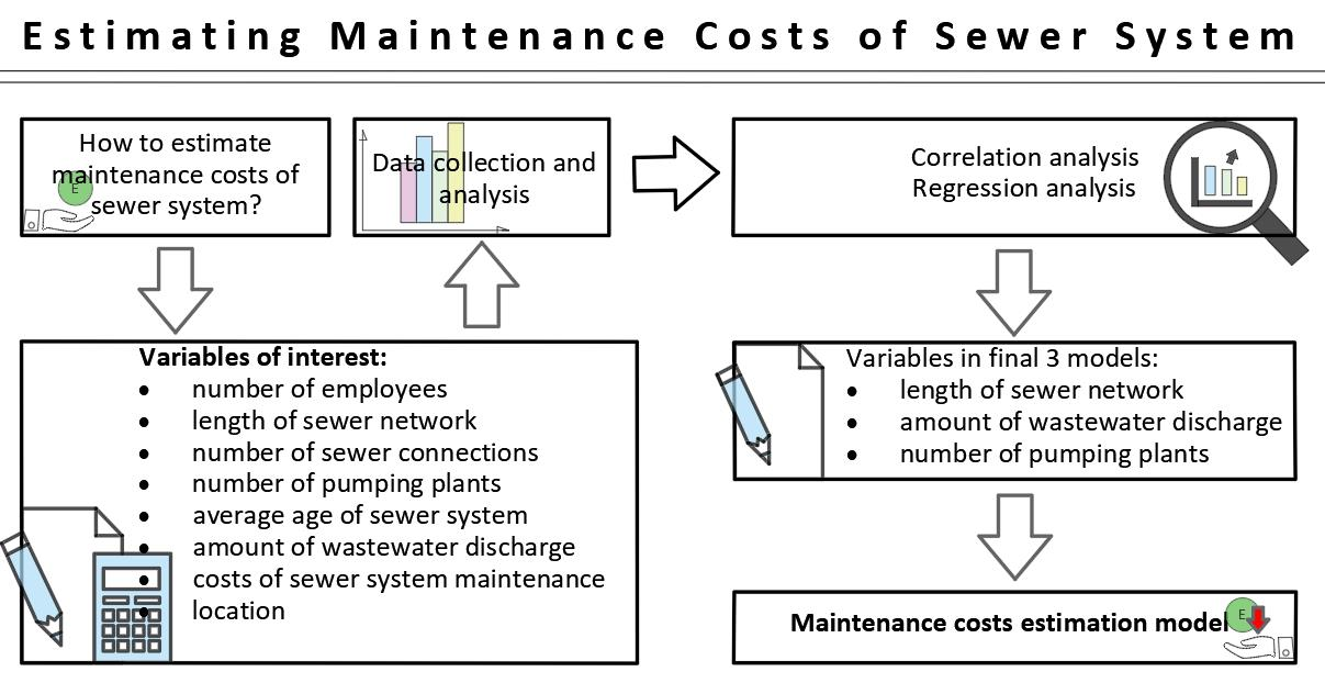
3. Data Collection and Analysis

In order to create the database necessary for drawing up a regression model for estimating the costs of sewer system maintenance, a questionnaire was created. Since the survey was conducted in 2019, data were requested as of 2018 because no complete data were available for 2019. The period for which the data were requested is 10 years, i.e., the first year was 2009 and the last was 2018.

In order to facilitate the collection of data on maintenance costs of a sewer system, the structure of costs and certain data on the functioning of the sewer system have been developed, as presented in

Table 2. Developed data structure and maintenance costs of sewerage system.

Number	Data
1	Maintenance costs of the sewerage system for each year [HRK], of which:
2	(a) machine work
3	(b) human work
4	(c) material
5	(d) other
6	Number of failures per year
7	The most frequent failures
8	Operating costs (electric energy) of pumping stations (HRK)
9	Maintenance costs of pump stations (HRK)
10	Costs of CCTV (Closed-circuit television) inspection (HRK)
11	How many km were inspected by CCTV
12	Costs of cleaning (flushing) sewerage system (HRK)
13	How many km have been cleaned (flushed)
14	Costs of trenchless rehabilitation (HRK)
15	How many km were rehabilitated with trenchless rehabilitation
16	Fuel consumed for maintenance (HRK) or (l)

. Collecting data on maintenance costs of the sewer system according to the structure below would enable annual monitoring of costs, as well as the development of more accurate models for estimating the costs of sewer system maintenance. All costs are given in Croatian kunas (HRK), the currency of Croatia when the research was conducted.

The values of certain characteristics of sewer systems for 2018 (the last year for which data on sewer systems were submitted using the questionnaires), such as the total length of the sewer network, the number of sewer connections, the number of wastewater treatment plants (WWTPs), and the amount of wastewater discharge, can also be seen as the scope of the conducted research. Data on these four characteristics for 2018 were downloaded from the official website of the Croatian Bureau of Statistics [42,43].

Data on the conducted research are given in

Table 3. Data on the scope of the conducted research.

Characteristics of Sewer System	Total in Year 2018 in Croatia [42,43]	Total for Completed Questionnaires Submitted	Share
Total length of sewer network [km]	12,529	2668.51	21.29%
Number of sewer connections [pcs]	587,922	132,240	22.49%
Number of WWTPs-a [pcs]	151	31	17.82%
Amount of wastewater discharge [m3]	335,807,000	38,304,853.15	11.41%

.

Independent variables, which can be considered important for defining the model for estimating maintenance costs of sewer system, have been defined from all data submitted, by analyzing the studies conducted so far, and by reviewing and analyzing the literature. The questionnaire sent to enterprises defines variables. The list of independent variables is given in

Table 4. List of possible independent variables in model for estimating maintenance costs of the sewerage system.

Number of Variable	Variable Name	Unit of Measurement	Type of Variable
1	Number of employees in sewerage system maintenance activities	pcs	discrete numerical
2	Total length of sewer network	km	continuous numerical
3	Total number of sewer connections	pcs	discrete numerical
4	Number of pumping plants	pcs	discrete numerical
5	Number of wastewater treatment plants (WWTPs)	pcs	discrete numerical
6	Average age of sewerage system	year	continuous numerical
7	Average annual amount of wastewater discharge	m3	continuous numerical
8	Average annual costs of sewerage system maintenance	HRK	continuous numerical
9	Location (land/sea)	-	qualitative

.

All valid and fully filled-in questionnaires produced a database that was used for statistical processing. For each sewer system, the total present value of the maintenance costs of the sewer system for the reference period, the average annual present value of maintenance costs and the average annual nominal maintenance costs were calculated. The total present value of maintenance costs was obtained by reducing the maintenance costs from the past to the present value according to the literature [44,45,46,47,48], while the discount rate was set at 3% for December 2021 according to [49,50].

A principle was adopted that assumed independent variables, such as the total length of the sewer network, the total number of sewer connections, and the number of pumping plants, did not change during the reference period. The same assumption was also adopted by Krstić [20] and Gudac Hodanić [41] in their doctoral dissertations.

4. Development of the Model for Estimating Maintenance Costs of the Sewer System

4.1. Regression Analysis

In order to develop a model for estimating maintenance costs, it is necessary to use certain independent variables to create a model for calculating the dependent variable—maintenance costs.

The software used in data processing is Statistica version 14.0.0.15. Statistica is a comprehensive analytical research and business tool. It is an integrated system that enables data management, analysis, data mining, visualization, and development of customized applications that contains a wide variety of basic and advanced analytical processes for business, data, scientific, and engineering applications. Statistica covers not only analytical, graphical, analytical, and database management processes, but also the extensive use of specialized data analysis methods. Input and output files and statistics charts can be virtually unlimited in size. Output reports can take the form of tables, workbooks, and reports [51].

In addition to the mentioned software, the programming language R was used. It is a programming language and environment for statistical calculations and visualization. It is available online under the general public license (GPL) so that it can be used and distributed freely and is open source [52,53,54]. The term “environment” suggests that this is a thoroughly planned and coherent system and not a gradual collection of very specific and inflexible tools, as is often the case with other data analysis software [55]. R offers a wide range of statistical methods for linear and non-linear modelling, classic statistical tests, analyses of time series, and clustering and is easily expandable with a wide selection of graphic techniques. Statisticians have developed many specialized statistical procedures for various uses through the so-called added packages that are available for free and integrated directly in the R system [54].

In general, regression analysis reveals relationships between the dependent and independent variables [56]. The data consist of continuous numerical and discrete numerical variables and the regression model for estimating maintenance costs will be developed. Whenever modelling is discussed, the aim of any model is to imitate the behaviour of the real system as best as possible, in this case, to assess maintenance costs. This characteristic, that is, the attribute that the model predicts the future state of the system, is called the predictive validity of the model [57]. The dependent variable is the one that is forecast [58] and is the independent variable by which it is forecast.

Regression analysis is the process of tuning functions into a partial dataset. Linear regression is the tuning of data with linear functions. This is achieved by using the least squares method [59]. The linear trend direction positioned between the (original) data sets using the least squares method should be positioned so that the sum of deviations of the original trend values is zero and that the sum of squares of these deviations is minimal [60].

Regression models can be used to predict the value of the dependent variable, given, of course, that the value of the independent variable is available [61]. The aim of the construction and use of the model is to create a simple model that will be easy to use, which will give a sufficiently close approximation of the complex reality. The model must be interpreted easily, but it must not be so simple as to ignore important influences.

A multiple linear regression model is the generalization of a simple linear regression so that there are several independent variables, instead of the one that occurs in simple linear regression. The aim of multiple linear regression is to explain and quantify the influence of several independent variables on one or more dependent variables.

The multiple linear regression model (according to [52,62,63,64]) is:

$$\mathrm{y}={\mathsf{\beta }}_0+{\mathsf{\beta }}_1{\mathrm{X}}_1+{\mathsf{\beta }}_2{\mathrm{X}}_2+\dots +{\mathsf{\beta }}_{\mathrm{n}}{\mathrm{X}}_{\mathrm{n}}+\mathsf{\epsilon }$$

(1)

where:

• y—dependent variable;
• X₁, X₂, …, Xn—independent variables;
• β₀, β₁, β₂, …, β_n—regression coefficients (constants);
• ε—random error (residual) [62].

Generally speaking, the model used should be as simple as possible.

Some of the advantages of simpler models—that is, models with less predictor variables—are as follows:

• Prevention of data adaptation—a data set with many dimensions that has many characteristics can sometimes lead the model to take into account both actual and accidental phenomena in the data.
• Interpretation—a model that is too complex and has too many characteristics is difficult to be interpreted, especially when compared to a simpler model.
• Computational efficiency—a model made on fewer dimensional data is more computationally efficient, i.e., it takes less time to be calculated [65]. Because of that, models with three or more variables are excluded from further analysis.

4.2. Accuracy of the Model

When considering the accuracy of the model, one of the two most frequently used indicators is the determination coefficient (R²) [66]. The coefficient of determination R² shows how many changes in experimental values of the dependent variable are explained by the obtained model [66,67,68]. When R² is near one, it says that the linear model explains a large portion of the dispersion in experimental values, i.e., only a small part remained unexplained by the model and should be attributed to a random error [66,68]. Hence, R² can serve as a criterion for selecting two models—a model that has a greater R² is better [69]. The size of R² can vary from zero to one [30]. An R² equal to one is an ideal link (regression) [70].

4.3. Correlation Coefficients of Variables

Table 5. Correlation coefficients of independent and dependent variables.

Variables	Number of Employees	Total Length of Sewer Network	Total Number of Sewer Connections	Number of Pumping Stations	Number of WWTPs	Average Age of Sewer system	Average Annual Amount of Waste Water Discharge	Average Annual Nominal Maintenance Costs	Average Present Value of Maintenance costs
Number of employees	1.000	0.694	0.878	0.486	0.452	0.327	0.666	0.525	0.520
Total length of sewer network	0.694	1.000	0.922	0.782	0.526	0.474	0.867	0.910	0.908
Total number of sewer connections	0.878	0.922	1.000	0.693	0.448	0.462	0.883	0.774	0.771
Number of pumping stations	0.486	0.782	0.693	1.000	0.763	0.376	0.742	0.584	0.582
Number of WWTPs	0.452	0.526	0.448	0.763	1.000	0.522	0.121	0.296	0.288
Average age of sewer system	0.327	0.474	0.462	0.376	0.522	1.000	0.235	0.455	0.451
Average annual amount of waste water discharge	0.666	0.867	0.883	0.472	0.121	0.235	1.000	0.792	0.793
Average annual nominal maintenance costs	0.525	0.910	0.774	0.584	0.296	0.455	0.792	1.000	1.000
Average present value of maintenance costs	0.520	0.908	0.771	0.582	0.288	0.451	0.793	1.000	1.000

shows the correlation coefficients for all observed independent variables and dependent variables, namely, the average annual present value of maintenance costs. As it can be seen in the table above, variables to be taken into account when drawing up the maintenance cost estimation model are those that have a higher correlation coefficient and where are (p < 0.05). There are four variables: the total length of the sewer network, the total number of sewer connections, the number of pumping stations and the average annual amount of waste water discharge. Correlations between the same variables are marked in yellow in the Table 5, and for them the correlation coefficient is 1.

Since there are four statistically significant variables (listed in

Table 6. Statistically significant independent variables for maintenance cost estimation model.

Name of Variable	p Value
Total length of sewer network	0.000044
Total number of sewer connections	0.003314
Number of pumping plants	0.047173
Average annual amount of wastewater discharge	0.002095

), models with a maximum of three variables were considered because the specified variables are correlated with each other. Therefore, having even greater correlation between two or more independent variables would make the estimated regression coefficients even less reliable [61].

The statistical significance of certain variables is less than 0.05, which means that the four variables listed are statistically significant.

Table 6 shows the p values of certain independent variables.

The Table 6 shows that the independent variable number of pumping plants is statistically significant (p = 0.0471 < 0.05), while the variables total number of sewer connections (p = 0.0033) and average annual amount of wastewater discharge (p = 0.0020) are very statistically significant (p < 0.01). The total length of the sewer network variable (p = 0.000044) is highly statistically significant at p < 0.001.

According to these four variables, several models for further elaboration will be proposed.

Table 7. Proposal for variables of the maintenance cost models with one variable.

Model Name	Variable Name in the Model	R2	Adjusted R2
Model 01	Total length of sewer network	0.8247	0.8072
Model 02	Total number of sewer connections	0.5948	0.5542
Model 03	Number of pumping plants	0.3386	0.2724
Model 04	Average annual amount of wastewater discharge	0.6287	0.5915

,

Table 8. Proposal for variables of the maintenance cost estimation models with two variables.

Model Name	Name of Variables in the Model	R2	Adjusted R2
Model 05	Total length of sewer network Total number of sewer connections	0.8549	0.8216
Model 06	Total length of sewer network Number of pumping plants	0.8673	0.8379
Model 07	Total length of sewer network Average annual amount of wastewater discharge	0.8248	0.7859
Model 08	Total number of sewer connections Number of pumping plants	0.5991	0.5099
Model 09	Total number of sewer connections Average annual amount of wastewater discharge	0.6514	0.5739
Model 10	Number of pumping plants Average annual amount of wastewater discharge	0.6839	0.6137

and

Table 9. Proposal for variables of the maintenance cost estimation models with three variables.

Model Name	Name of Variables in the Model	R2	Adjusted R2
Model 11	Total length of sewer network Total number of sewer connections Number of pumping plants	0.9062	0.8710
Model 12	Total number of sewer connections Number of pumping plants Average annual amount of wastewater discharge	0.6840	0.5655
Model 13	Total length of sewer network Number of pumping plants Average annual amount of wastewater discharge	0.8955	0.8564
Model 14	Total length of sewer network Total number of sewer connections Average annual amount of wastewater discharge	0.8631	0.8118

provide the values of the coefficient of determination (R²) and the values of the adjusted coefficient of determination (adjusted R²).

As there are four statistically significant variables, models with no more than three variables were considered because certain variables listed below are correlated and the estimated regression coefficients would be all less reliable in case of a greater correlation between two or more independent variables [61].

4.4. Proposal for Variables of Maintenance Cost Estimation Models

Models, i.e., names of variables in the model under consideration, are presented in Table 7, Table 8 and Table 9.

If all variables are included in the model, as in this case, R² is 0.9757 and the value of the adjusted coefficient of determination (adjusted R²) is 0.9332.

By adding an additional independent variable to the multiple regression model, it can happen that non-significant variables occur, and it is usually the case that R² dramatically increases [61]. From this, it can be observed that when all independent variables are included in the multiple linear regression model, R² = 0.9757 and the adjusted R² = 0.9332; and these are the highest values of both indicators that can be achieved by the model. Therefore, the R² values and the adjusted R² values given in Table 7, Table 8 and Table 9 are acceptable and fine, since the proposed models have one, two or a maximum of three variables, which is less than the maximum number of variables included in the model. Therefore, the values of the two above coefficients are at their highest values.

Figure 2 shows the coefficient of determination (R²) and the adjusted coefficient of determination (adjusted R²) for all 14 models proposed in the tables above. Those for model 15 are also given below and shown on Figure 2.

Table 10. MAE and AIC values for the proposed models.

Model Name	MAE	AIC
Model 01	533,998.4	360.44
Model 02	685,501.3	370.49
Model 03	802,015.7	376.37
Model 04	583,127.2	369.44
Model 05	476,325.1	360.24
Model 06	427,782.2	359.09
Model 07	531,263.6	362.43
Model 08	698,981.9	372.36
Model 09	592,805.5	370.68
Model 10	609,270.9	369.51
Model 11	377,459.6	356.93
Model 12	607,508.4	371.50
Model 13	405,506.6	358.22
Model 14	433,878.3	361.46

shows the mean absolute error (MAE) and Akaike information criterion (AIC) values.

For previously proposed model variables, the mean absolute error (MAE) and the Akaike information criterion (AIC) [71] were calculated. The mean absolute error is relatively easy to calculate. It is a measure of the accuracy indicator of the model, and according to [72], it is recommended as a measure of deviation. The AIC was proposed by Hirotugu Akaike [73,74,75] and the objective of selecting the model using AIC criteria is to estimate the loss of information so that the model with the lowest expected loss of information is equivalent to selecting the model with the lowest AIC value [76]. Therefore, the use of AIC reduces the possibility of model overfitting and decreases the number of variables. It helps to identify and compare the best models and “punishes” models with more than one variable, since a model with more than one variable is known to have a better match with the data, creating a risk of model overadjustment [77].

In addition to these 14 models, a model with interactions was made (model 15). In general, two variables, X1 and X2, are said to be interacting if the value of variable X1 affects the value of variable X2 positively or negatively. The interaction is synergy between two or more variables and reflects the fact that their combined effect on the response (result) depends not only on the values of individual variables, but also on their combinations of values [78].

The interaction refers to the fact that the magnitude (value) of the influence of an independent variable on the response depends on a certain value of another independent variable [64]; in short, this means that there is a dependence of one predictor variable on the value of another predictor variable [79].

It can be seen that the position variable, which has two or three possible values (“mainland little”—sewer systems in continental Croatia less than 200 km long; “mainland large”—sewer systems in continental Croatia over 200 km long; and “sea”—sewer systems in coastal Croatia regardless of length) has not yet been taken into account anywhere. The name of the “mainland little” variable will be given to all sewer systems with a total length of sewer network of less than 200 km and located in continental Croatia, the “mainland large” are sewer systems in continental Croatia with a length of over 200 km and the “sea” variable is for all those sewer systems located in coastal Croatia. These values (mainland small, mainland large, sea) were obtained by a more careful analysis of the dispersion diagram for maintenance costs variables and the total length of the sewer net-work. Sewer systems in coastal Croatia show a different regression direction in relation to the regression direction for continental Croatia. For continental Croatia, there is a difference in regression direction for the total length of sewer systems that are 200 km long and those with a length greater than 200 km [19].

For model 15, data on the coefficient of determination R², the adjusted coefficient of determination (adjusted R²), MAE and AIC are given in

Table 11. Data for the model with interactions (Model 15).

Model Name	R2	Adjusted R2	MAE	AIC
Model 15	0.9238	0.8603	302,873.3	358.44

.

4.5. Selected Maintenance Cost Estimation Models

Based on all the above, four finally selected models are presented in

Table 12. Variables of the maintenance cost estimation model with the corresponding data.

Model Name	Variable(s) in Model	R2	Adjusted R2	MAE	AIC
Model 01	Total length of sewer network	0.8247	0.8072	533,998.4	360.44
Model 04	Average annual amount of wastewater discharge	0.6287	0.5915	583,127.2	369.44
Model 06	Total length of sewer network Number of pumping plants	0.8673	0.8379	427,782.2	359.09
Model 15	Total length of sewer network Position	0.9238	0.8603	302,873.3	358.44

.

When considering the values of the R² coefficient of determination and the adjusted coefficient of determination in Table 12, it is evident that all proposed models have satisfactory values of coefficients for further analysis. The MAE and AIC values are presented and are satisfactory with respect to model 11, which has three independent variables and whose AIC value is the smallest of the 15 models observed; moreover, model 15 has the smallest MAE value of all 15 models observed. With regard to these two models, the concept of satisfactory values has been defined. In order to make the final selection of the model for estimating the maintenance costs of the sewer system, validation of all models on the test sample will be made.

Regression coefficients and constants were obtained via regression analysis in programming language R and Statistica software.

Table 13. Summary overview of developed models.

Model Name	Model Equation	Input Data
Model I	AANMC = −406158.2 + 6321.7 × TLSN	length of sewer network
Model II	AANMC = 130800 + 0.2853 × AWD	annual amount of wastewater
Model III	AANMC = −250789 + 8129 × TLSN – 1515 × NPP	length of sewer network number of pumping plants
Model IV	AANMC = −409506 + 10266 × TLSN	length of sewer network <200 km, mainland
	AANMC = −2306094 + 10678 × TLSN	length of sewer network >200 km, mainland
	AANMC = −256960 + 6582 × TLSN	length of sewer network regardless of length, sea

Where:

• AANMC, average annual nominal maintenance costs;
• TLS_N, total length of sewer network;
• AWD, the average annual amount of wastewater discharge;
• NPP, number of pumping plants.

presents the model name, equation for model and input data, i.e., input variables, of the developed models.

5. Validation of the Models for Estimating Maintenance Costs of a Sewer System

The validation of the model is an important part of the design of the regression model [80] and it is the last step in its construction. The validation gives final approval for the model in the sense that it confirms that it can be used to predict the variable of interest, namely, the data to be envisaged [62,81]. The validation is a comparison of prediction results using a model with actual results to see if the model is suitable for the intended purpose [72,82].

The validation of the model is conducted for the following reasons: to select the best model, as a measure of the accuracy of the model and for statistical reasons, i.e., to identify the model that has the least error [83].

The purpose of validation of the obtained model is to:

• Ensure the feasibility of the model in the future, i.e., that the model can be used in the future using new data similar to those used in the construction of the model [84,85].
• Avoid overfitting—the phenomenon where the model is suitable only for the dataset used in the construction of the model (the relearned model is a model that has more parameters than can be justified)—and underfitting [85] (the phenomenon where the built model lacks certain parameters, the model does not describe data well or when independent variables are not significant enough in defining the link between dependent and independent variables) [86].

In order to validate the model and determine the applicability of the model for estimating the maintenance costs of the sewer system, four models were used to estimate maintenance costs on the sewer system intended for validation. The selected sewer system is on land and over 200 km long. The sewer system intended for validation is, according to all characteristics, suitable for validation because it is located in the continental part of the Republic of Croatia and the independent variables are within the data range used for modeling. Using the regression model (extrapolation) outside the range of the data values used for estimation is not recommended [61], i.e., the use of the regression equation outside the data domain used is risky [87]. For these reasons, it has been decided that this model will be used to validate the constructed models.

The average annual amount of waste water discharge was obtained in such a way that, for all the years for which data on the annual amount of waste water were submitted, the total amount of waste water was divided by the number of years, i.e., an average was obtained. In addition, an average of the sum of all maintenance costs for the years for which the data were submitted was calculated to obtain the average annual maintenance costs.

For validation, an expression will be used to calculate the accuracy of the model (model accuracy, A_C), which is calculated as a percentage of the difference between the value of the model costs and the value of the actual costs. The closer Ac is to zero, the more accurate the model is.

The expression for the accuracy of the model (according to [2]) is as follows:

$${\mathrm{A}}_{\mathrm{C}}=\left[\frac{\mathrm{PC}-\mathrm{AC}}{\mathrm{AC}}\right]\times 100\%$$

(2)

where:

• Ac, accuracy of calculated costs;
• PC, costs predicted by the model;
• AC, real costs.

The validation results of four models are presented in the

Table 14. Validation results of four models on the test sample.

Model Name	Actual Value (HRK)	Estimated Value (HRK)	Accuracy of the Model, Ac
Model I	1,564,276.60	1,420,813.10	−9.17%
Model II		1,500,127.22	−4.10%
Model III		2,053,042.00	+31.24%
Model IV		779,848	−50.15%

. The estimated value obtained is the average cost value for one year of sewer system maintenance.

To conclude, both models (model I and model II) are found to be suitable for use considering the accuracy obtained for validation on the test sample. In addition, model III is appropriate for use, and the estimated amount of maintenance costs generated by this model should be on the side of safety, as the amount obtained is overestimated (exceeded). Using such a model, the estimated maintenance cost is higher than the actual maintenance cost. However, it is important to take into account that all three models provide average annual maintenance costs for the sewer system, and since these are average costs, it is clear that costs may be lower or higher than this average value. Therefore, it is possible that in a given year the costs that are now higher will be closer to this estimated value in the future. Therefore, the use of this model is also justified.

6. Discussion

For the quantification of correlations between dependent and independent variables, the following values of the Pearson correlation coefficient between dependent variables are calculated: average annual present values of maintenance costs, average annual nominal maintenance costs and any independent variables. The analysis has found that there are a few more apparent correlations between independent variables and maintenance costs.

The maintenance costs of the sewer system have the highest correlation with the following independent variables:

• The total length of the sewer system;
• The number of sewer connections;
• The number of pumping plants; and
• The average annual amount of waste water discharge.

The most significant correlation with the total length of the sewer system is to be expected since it is, to some extent, one of the most important characteristics of the sewer system. This is also the case with an average annual amount of waste water discharge, such as in residential buildings; the surface of rooms is one of the most important characteristics of the building itself. The total length of the sewer system and the average annual amount of wastewater discharge show a significant correlation with maintenance costs.

The advantage of using the cost estimation model for the maintenance of the sewer system is the simplicity of its use. The variable needed to estimate costs is the total length of the sewer network or the average annual amount of wastewater discharge. Both models can be chosen according to what data are available. In addition, the third variable is the position where the sewer system is located and its length (whether it is up to 200 km long or over 200 km long—only valid for sewer systems in continental parts as in coastal Croatia, the length of the position variable is not important). The fourth variable that can be taken into account is the number of pumping plants, which is also available in the design phase of the sewer system. These variables are available at the beginning of the planning and construction of the drainage system. Because of the above, it is possible to estimate the maintenance costs of the sewer system using this model. The result of using the maintenance cost estimation model for the sewer system is the value of its average annual maintenance costs that are the same for each maintenance year in the observed reference period.

The first and the most important limitation of the model is the smaller amount of data on which the model has been developed and validated. Cost data are typically considered a business secret, which, as expected, made it very difficult to collect data. In addition, cost records kept by companies in charge of the management of sewer systems are, in most cases, incomplete, inaccurate or difficult to obtain.

The second limitation relates to the number of years for which the maintenance costs of the sewer system are estimated. The period for which data on the sewer system maintenance costs have been provided ranges from 2 to 10 years; in this respect, costs can be estimated for a maximum period of 10 years. The calculated regression equation is valid for a given area that is bounded by the minimum and maximum values of the dependent and independent variables, and the use of the model equation outside that area is risky [87].

The third limitation is related to the values of independent variables by which the dependent variable—the maintenance costs of the sewer system— is estimated. All independent variables should be in the range of data used in modelling; otherwise, the use of such a model is not advisable. An independent variable used to model the maintenance cost estimation of the sewer system is the average annual amount of wastewater discharge from 4197.33 m³ to 14,223,945 m³, which indicates that a model can be used for such data ranges. In addition, the second independent variable, the sewer system’s length, has taken values from 5.1 km to 752.42 km, indicating that the model can be used in this range. The third independent variable ranged from 1 pumping plant to a maximum of 92 pumping plants, indicating that the model can be applied for ranges within the above values. Overall, all three ranges of independent variables are large, so it is to be considered that all three models, depending on which independent variables they take into account, can be used in the data ranges given above.

7. Conclusions

The literature review and analysis developed an appropriate structure of maintenance costs for sewer systems to facilitate the systematization of these costs, i.e., using data for each year from companies in charge of the management and maintenance of sewer systems. The structure of maintenance costs of the sewer system has also been developed. The developed sewer system maintenance cost structure can help collect data and develop more accurate models for estimating the maintenance costs of sewer systems.

After the 15 preliminary models were prepared, according to the adjusted R², the MAE and AIC criteria were used to decide on the models to be considered further. Based on the above criteria, four models were selected. After their validation, a model was adopted where the independent variable is the average annual amount of waste water discharge. However, the model with the total length of the sewer system as an independent variable could also be used, as it shows a satisfactory accuracy of −9.17% on the test sample. This sample was left just for model validation. The model is more accurate as the accuracy value is closer to zero, as already mentioned. The model with the total length of the sewer system for the independent variable has a coefficient of determination R² = 0.8247, and the model with the average annual amount of wastewater discharge as the independent variable has a coefficient of determination R² = 0.6287.

By selecting significant variables, models were made to estimate the maintenance cost of a sewer system. The models were constructed using linear regression and were validated on a test sample. The model using the total length of the sewer system as the independent variable provides an accuracy of −9.17%; the model using the average annual amount of wastewater discharge as the independent variable has an accuracy of −4.10%; and the model using the total length of the sewer system and the number of pumping plants as the independent variables has an accuracy of +31.24%.

The first two models (model I and model II) are applicable to estimating the maintenance costs of a sewer system, while the third model (model III) is also applicable since it uses two independent variables and, in certain cases, where the total length of sewer system and the number of pumping plants are known, could give a better assessment than the others. The third model gives higher estimates, so the user of such a model should err on the side of caution.

Certainly, when using the estimation model, the recommendation would be that an assessment be made according to all three models and that the value of maintenance cost estimation be greater than needed or that a decision be made based on previous values of maintenance costs of the observed sewer system should the sewer system be already in use. Of course, the model for estimating the maintenance cost of a sewer system has the highest value for those sewer systems that are only in the design phase or are being built, in which case the maintenance costs can be estimated in the future to plan a certain maintenance budget.

It has been established that the characteristics most affected by the maintenance costs of sewer system are as follows: the total length of sewer network, the average annual amount of wastewater discharge, the number of pumping plants and the location (i.e., is the sewer system in coastal or continental Croatia).

The main advantage of applying this model for estimating the maintenance costs of a sewer system is its simplicity, which is one characteristic of a good model. The variable required to estimate costs is the total length of the sewer network or the average annual amount of wastewater discharge. It is possible to use both models depending on the data available or to compare the estimations of maintenance costs obtained through each one to select a more critical maintenance cost value.

The use of the maintenance cost assessment model opens up new possibilities in planning the necessary budget for sewer system maintenance, thus making maintenance more efficient. Companies operating the sewer system of a city, settlement or municipality may include in their budget the average necessary amount to be spent annually on sewer system maintenance.

Consequently, this model could also be used by the companies responsible for sewer system management to assess the funds needed for sewer maintenance in the area in which they operate.

8. Recommendations for Future Research

Since research of this kind on the maintenance costs of sewer systems has not yet been conducted in the Republic of Croatia, this study can serve as the basis for further research. In order to obtain the most reliable results, it is necessary to investigate a large number of cases (larger sample), i.e., to expand the research to several companies in the territory of the Republic of Croatia. It is necessary to raise the level of awareness of project engineers and persons who manage the maintenance of sewer systems about the life cycle costs of sewer systems, including maintenance costs.

Anything relating to money is or can be considered a business secret by both private and public institutions. Therefore, it is necessary to reduce or eliminate the resistance of institutions to providing such data for scientific and research purposes. If these maintenance cost data were made more readily available, this would benefit all stakeholders greatly, as it would allow for the comparison and development of certain models to assess or forecast costs, leading to more efficient maintenance. In addition, the time limit for applicability of the constructed maintenance cost estimation model may be tested.

It is possible to develop a certain information system on the national level in the Republic of Croatia or even the European Union, where all companies managing sewer systems would enter certain characteristics of their sewer systems such as the maintenance costs for a certain period, etc. This would make it possible to compare the quality of maintenance, maintenance costs and, finally, to develop the most accurate model for estimating the maintenance costs of sewer systems.

References

- Marenjak, S.; El-Haram, M.A.; Horner, R.M.W. Procjena ukupnih troškova projekata u visokogradnji. J. Croat. Assoc. Civ. Eng. 2002, 54, 393–401. [Google Scholar]
- Al-Hajj, A.; Horner, M.W. Modelling the running costs of buildings. Constr. Manag. Econ. 1998, 16, 459–470. [Google Scholar] [CrossRef]
- Du, W.; Yu, J.; Gu, Y.; Li, Y.; Han, X.; Liu, Q. Preparation and application of microcapsules containing toluene-di-isocyanate for self-healing of concrete. Constr. Build. Mater. 2019, 202, 762–769. [Google Scholar] [CrossRef]
- Van Belleghem, B.; Van Tittelboom, K.; De Belie, N. Efficiency of self-healing cementitious materials with encapsulated polyurethane to reduce water ingress through cracks. Mater. Construcción 2018, 68, e159. [Google Scholar] [CrossRef]
- Gardner, D.; Lark, R.; Jefferson, T.; Davies, R. A survey on problems encountered in current concrete construction and the potential benefits of self-healing cementitious materials. Case Stud. Constr. Mater. 2018, 8, 238–247. [Google Scholar] [CrossRef]
- Danish, A.; Mosaberpanah, M.A.; Usama Salim, M. Past and present techniques of self-healing in cementitious materials: A critical review on efficiency of implemented treatments. J. Mater. Res. Technol. 2020, 9, 6883–6899. [Google Scholar] [CrossRef]
- Tafuri, A.N.; Selvakumar, A. Wastewater collection system infrastructure research needs in the USA. Urban Water 2002, 4, 21–29. [Google Scholar] [CrossRef]
- United States General Accounting Office. WATER INFRASTRUCTURE Comprehensive Asset Management Has Potential to Help Utilities Better Identify Needs and Plan Future Investments; United States General Accounting Office: Washington, DC, USA, 2004. [Google Scholar]
- Kujundžić, B. Kanalizacioni sistem—Definicija, karakteristike, delovi i zadaci. In Savremena Eksploatacija i Održavanje Objekata i Opreme Vodovoda i Kanalizacije; Kujundžić, B., Ed.; Udruženje za tehnologiju vode i sanitarno inženjerstvo: Beograd, Serbia, 2010; pp. 345–354. ISBN 978-86-82931-33-1. [Google Scholar]
- Obradović, D. Prevencija kvarova sprječavanjem rasta i uklanjanjem korijenja drveća u kanalizacijskim cijevima. Vodoprivreda 2018, 50, 165–173. [Google Scholar]
- Marsalek, J.; Schillling, W. Operation of sewer systems. In Hydroinformatics Tools for Planning, Design, Operation and Rehabilitation of Sewer Systems; Marsalek, J., Maksimovic, C., Zeman, E., Price, K.R., Eds.; Kluwer Academic Publishers: Dordrecht, The Netherlands, 1998; pp. 393–414. [Google Scholar]
- American Society of Civil Engineers (ASCE). 2021 Infrastructure Report Card; American Society of Civil Engineers (ASCE): Reston, VA, USA, 2021. [Google Scholar]
- American Society of Civil Engineers (ASCE). 2017 Infrastructure Report Card; American Society of Civil Engineers (ASCE): Reston, VA, USA, 2017. [Google Scholar]
- Đorđević, B. Cybernetics in Water Resources Management; Water Resources Publication: Littleton, CO, USA, 1993. [Google Scholar]
- Karić, M. Mikroekonomika; Dotiskano prvo izdanje; Ekonomski fakultet u Osijeku: Osijek, Croatia, 2009. [Google Scholar]
- Tayefeh Hashemi, S.; Ebadati, O.M.; Kaur, H. Cost estimation and prediction in construction projects: A systematic review on machine learning techniques. SN Appl. Sci. 2020, 2, 1703. [Google Scholar] [CrossRef]
- CPHEEO. Manual on Sewerage and Sewage Treatment Systems; Ministry of Urban Development, New Delhi; Central Public Health and Environmental Engineering Organization in collaboration with Japan International Cooperation Agency: Chennai, India, 2013. [Google Scholar]
- Paulson, B.C. Designing to Reduce Construction Costs. J. Constr. Div. 1976, 102, 587–592. [Google Scholar] [CrossRef]
- Obradović, D. Doprinos Povećanju Učinkovitosti Održavanja Kanalizacijskih Sustava Primjenom Modela Procjene Troškova, Održavanja. Ph.D. Thesis, Sveučilište Josipa Jurja Strossmayera u Osijeku, Građevinski i arhitektonski fakultet Osijek, Osijek, Croatia, 2022. [Google Scholar]
- Krstić, H. Model Procjene Troškova Održavanja i Uporabe Građevina na Primjeru Građevina Sveučilišta Josipa Jurja Strossmayera u Osijeku. Ph.D. Thesis, Sveučilište Josipa Jurja Strossmayera u Osijeku, Građevinski fakultet Osijek, Osijek, Croatia, 2011. [Google Scholar]
- Waier, R.P.; Plotner, C.S. Chapter 15—Maintenance & Repair Estimating. In RS Means: Cost Planning & Estimating for Facilities Maintenance; Waier, R.P., Plotner, C.S., Morris, S., Eds.; John Wiley & Sons: Hoboken, NJ, USA, 1996; pp. 231–251. ISBN 978-0-87629-419-2. [Google Scholar]
- Wood, B. Building Care; Blackwell Science Ltd.: Oxford, UK, 2003; ISBN 0-632-06049-2. [Google Scholar]
- Aziz, A.M.A. Performance Analysis and Forecasting for WSDOT Highway Projects; Washington State Transportation Center (TRAC): Seattle, WA, USA, 2007. [Google Scholar]
- Cheung, F.K.T.; Skitmore, M. Application of cross validation techniques for modelling construction costs during the very early design stage. Build. Environ. 2006, 41, 1973–1990. [Google Scholar] [CrossRef]
- Liu, Y. A Forecasting Model for Maintenance and Repair Costs for Office Buildings; Concordia University: Montreal, Canada, 2006. [Google Scholar]
- Shah, A.A.; Ahmad, F.; Peng Au-Yong, C. Office building maintenance: Cost prediction model. J. Croat. Assoc. Civ. Eng. 2013, 65, 803–809. [Google Scholar] [CrossRef]
- Marenjak, S.; Krstić, H. Analysis of buildings operation and maintenance costs. J. Croat. Assoc. Civ. Eng. 2012, 64, 293–303. [Google Scholar] [CrossRef]
- Krstić, H.; Marenjak, S. Maintenance and operation costs model for university buildings. Teh. Vjesn. 2017, 24, 193–200. [Google Scholar] [CrossRef]
- Lee, C.-K.; Jeon, Y.-I. A maintenance cost prediction model for elementary schools by correcting FM budget history and performance data. Int. J. Appl. Or Innov. Eng. Manag. 2017, 6, 084–094. [Google Scholar]
- Boussabaine, A.H.; Kirkham, R.J. Simulation of maintenance costs in UK local authority sport centres. Constr. Manag. Econ. 2004, 22, 1011–1020. [Google Scholar] [CrossRef]
- Kim, J.-M.; Kim, T.; Yu, Y.-J.; Son, K. Development of a Maintenance and Repair Cost Estimation Model for Educational Buildings Using Regression Analysis. J. Asian Archit. Build. Eng. 2018, 17, 307–312. [Google Scholar] [CrossRef]
- Mahmoud, S.; Khamidi, M.F.; Idrus, A.; Abdul-Lateef Ashola, O. Development of Maintenance Cost Prediction Model for Heritage Buildings. J. Teknol. 2015, 74, 51–57. [Google Scholar] [CrossRef]
- Nipp, T.J. Development of a Mathematical Model for the Estimation of Required Maintenance for a Homogenous Facilities Portfolio Using Multiple Linear Regression. Ph.D. Thesis, University of Tennessee, Knoxville, TN, USA, 2017. [Google Scholar]
- Tijanić Štrok, K. Razvoj Modela za Učinkovito Upravljanje Održavanjem Javnih Obrazovnih Građevina. Ph.D. Thesis, Sveučilište Josipa Jurja Strossmayera u Osijeku, Građevinski i arhitektonski fakultet Osijek, Osijek, Croatia, 2021. [Google Scholar]
- Bouabaz, M.; Horner, R.M.W. Modelling and Predicting Bridge Repair and Maintenance Costs. In Bridge Management; Springer US: Boston, MA, USA, 1990; pp. 187–197. [Google Scholar]
- Shi, X.; Zhao, B.; Yao, Y.; Wang, F. Prediction Methods for Routine Maintenance Costs of a Reinforced Concrete Beam Bridge Based on Panel Data. Adv. Civ. Eng. 2019, 2019, 5409802. [Google Scholar] [CrossRef]
- Li, C.-S.; Guo, S.-J. Development of a Cost Predicting Model for Maintenance of University Buildings. In Proceedings of the 2011 2nd International Congress on Computer Applications and Computational Science: Volume 1; Springer: Berlin/Heidelberg, Germany, 2012; pp. 215–221. [Google Scholar]
- Li, C.-S.; Guo, S.-J. Life Cycle Cost Analysis of Maintenance Costs and Budgets for University Buildings in Taiwan. J. Asian Archit. Build. Eng. 2012, 11, 87–94. [Google Scholar] [CrossRef]
- Bouabaz, M.; Hamami, M. A Cost Estimation Model for Repair Bridges Based on Artificial Neural Network. Am. J. Appl. Sci. 2008, 5, 334–339. [Google Scholar] [CrossRef]
- Asadi, A.; Hadavi, A.; Krizek, R.J. Bridge Life-Cycle Cost Analysis Using Artificial Neural Networks. In Proceedings of the CIB W78-W102 2011: International Conference, Sophia Antipolis, France, 26–28 October 2011. [Google Scholar]
- Gudac Hodanić, I. Model Procjene Troškova Životnog Ciklusa Pontona Kao Podrška Sustavu Upravljanja Marinama. Ph.D. Thesis, Sveučilište Josipa Jurja Strossmayera u Osijeku, Građevinski i arhitektonski fakultet Osijek, Osijek, Croatia, 2020. [Google Scholar]
- Državni Zavod za Statistiku Republike Hrvatske. “Tablica 1.3. Mreža Javne Odvodnje i Uređaji za Pročišćavanje Otpadnih Voda”, Zagreb. 2021. Available online: https://web.dzs.hr/PXWeb/Selection.aspx?px_path=Okolis__Statistika%20voda__Javna%20odvodnja&px_tableid=JO13.px&px_language=hr&px_db=Okolis&rxid=3f60bc89-c4fe-4ab8-a06a-29a5d62adbf5 (accessed on 8 November 2022).
- Državni Zavod za Statistiku Republike Hrvatske. “Tabela 1.1. Podrijetlo, Pročišćavanje i Ispuštanje Otpadih voda, tis. m3”, Zagreb. 2022. Available online: https://web.dzs.hr/PXWeb/Selection.aspx?px_path=Okolis__Statistika%20voda__Javna%20odvodnja&px_tableid=JO11.px&px_language=hr&px_db=Okolis&rxid=3f60bc89-c4fe-4ab8-a06a-29a5d62adbf5 (accessed on 8 November 2022).
- Medanić, B.; Pšunder, I.; Skendrović, V. Neki Aspekti Financiranja i Financijskog Odlučivanja u Građevinarstvu; Sveučilište Josipa Jurja Strossmayera u Osijeku, Građevinski fakultet: Osijek, Croatia, 2005. [Google Scholar]
- Čulo, K. Ekonomika Investicijskih Projekata; Građevinski fakultet Osijek: Osijek, Croatia, 2010. [Google Scholar]
- Van Horne, C.J.; Wachowicz, M.J. Osnove Financijskog Menadžmenta; Trinaesto izdanje; MATE d.o.o. Zagreb, ZŠEM: Zagreb, Croatia, 2014. [Google Scholar]
- Salvatore, D. Ekonomija za Menadžere u Svjetskoj Privredi; MATE d.o.o. Zagreb: Zagreb, Croatia, 1994. [Google Scholar]
- Samuelson, A.P.; Nordhaus, D.W. Ekonomija; petnaesto; MATE d.o.o. Zagreb: Zagreb, Croatia, 2000. [Google Scholar]
- Hrvatska narodna banka. Tablica F1: Aktivne Kamatne Stope Hrvatske Narodne Banke; Hrvatska narodna banka: Zagreb, Croatia, 2021. [Google Scholar]
- Narodne Novine. Odluka o Kamatnim Stopama, Diskontnoj (Eskontnoj) Stopi i Naknadama Hrvatske Narodne Banke; Narodne novine, Službeni list Republike Hrvatske: Zagreb, Croatia, 2017. [Google Scholar]
- TIBCO Software Inc. TIBCO Statistica Quick Reference; TIBCO Software Inc.: Palo Alto, CA, USA, 2018. [Google Scholar]
- Dalgaard, P. Introductory Statistics with R; Springer: New York, NY, USA, 2008. [Google Scholar]
- Schumacker, R.; Tomek, S. Understanding Statistics Using R; Springer: New York, NY, USA, 2013. [Google Scholar]
- Radović, A. Upoznavanje sa Sintaksom Jezika R i Njegova Primjena u Uosnovnoj Statističkoj i Grafičkoj Analizi Podataka; Sveučilište u Zagrebu, Sveučilišni računski centar: Zagreb, Croatia, 2015. [Google Scholar]
- Venables, W.N.; Smith, D.M.; the R Core Team. An Introduction to R, Notes on R: A Programming Environment for Data Analysis and Graphics; Version 4. 2022. Available online: https://cran.r-project.org/doc/manuals/r-release/R-intro.pdf (accessed on 21 August 2021).
- Taha, A.H. Operations Research: An Introduction, 7th ed.; Pearson Education International: London, UK, 2003. [Google Scholar]
- Čerić, V. Simulacijsko Modeliranje; Školska knjiga: Zagreb, Croatia, 1993. [Google Scholar]
- Novaković, V. Kvantitativni Metodi u Građevinskom Menadžmentu; Časopis “Izgradnja” Saveza građevinskih Inženjera i tehničara Srbije, Saveza arhitekata Srbije, društva za mehaniku tla i fundiranje Srbije, Udruženja urbanista Srbije: Beograd, Serbia, 2002. [Google Scholar]
- Barnett, A.R.; Ziegler, R.M.; Byleen, E.K. Primjenjena Matematika za Poslovanje, Ekonomiju, Znanosti o Živom Svijetu i Humanističke Znanosti; MATE d.o.o. Zagreb: Zagreb, Croatia, 2006. [Google Scholar]
- Galić, R. Statistika; Elektrotehničku fakultet, Sveučilište Josipa Jurja Strossmayera u Osijeku: Osijek, Croatia, 2004. [Google Scholar]
- Newbold, P.; Carlson, J.W.; Thorne, M.B. Statistika za Poslovanje i Ekonomiju; šesto izda; MATE d.o.o. Zagreb: Zagreb, Croatia, 2010; ISBN 978-953-246-083-4. [Google Scholar]
- Rodríguez del Águila, M.M.; Benítez-Parejo, N. Simple linear and multivariate regression models. Allergol. Immunopathol. 2011, 39, 159–173. [Google Scholar] [CrossRef]
- Grégoire, G. Multiple Linear Regression. EAS Publ. Ser. 2014, 66, 45–72. [Google Scholar] [CrossRef]
- Fitzmaurice, G.M. Regression. Diagn. Histopathol. 2016, 22, 271–278. [Google Scholar] [CrossRef]
- Obi Tayo, B. Simplicity vs Complexity in Machine Learning—Finding the Right Balance. 2019. Available online: https://towardsdatascience.com/simplicity-vs-complexity-in-machine-learning-finding-the-right-balance-c9000d1726fb. (accessed on 24 August 2021).
- James, G.; Witten, D.; Hastie, T.; Tibshirani, R. An Introduction to Statistical learning with Applications in R; Springer US: Los Angeles, CA, USA, 2013. [Google Scholar]
- Serdar, V. Udžbenik Statistike; Školska knjiga: Zagreb, Croatia, 1966. [Google Scholar]
- Benšić, M.; Šuvak, N. Primijenjena Statistika; Sveučilište, J.J., Ed.; Strossmayera u Osijeku, Odjel za matematiku: Osijek, Croatia, 2013. [Google Scholar]
- Merkle, M. Verovatnoća i Statistika za Inženjere i Studente Tehnike; Akademska misao: Beograd, Serbia, 2002. [Google Scholar]
- Unpingco, J. Python for Probability, Statistics, and Machine Learning; Springer International Publishing: Cham, Germany, 2019; ISBN 978-3-030-18544-2. [Google Scholar]
- Forster, M.R. Key Concepts in Model Selection: Performance and Generalizability. J. Math. Psychol. 2000, 44, 205–231. [Google Scholar] [CrossRef]
- Mayer, D.G.; Butler, D.G. Statistical validation. Ecol. Modell. 1993, 68, 21–32. [Google Scholar] [CrossRef]
- Akaike, H. Factor analysis and AIC. Psychometrika 1987, 52, 317–332. [Google Scholar] [CrossRef]
- Bozdogan, H. Model selection and Akaike’s Information Criterion (AIC): The general theory and its analytical extensions. Psychometrika 1987, 52, 345–370. [Google Scholar] [CrossRef]
- Cavanaugh, J.E.; Neath, A.A. The Akaike information criterion: Background, derivation, properties, application, interpretation, and refinements. WIREs Comput. Stat. 2019, 11, e1460. [Google Scholar] [CrossRef]
- Wagenmakers, E.-J.; Farrell, S. AIC model selection using Akaike weights. Psychon. Bull. Rev. 2004, 11, 192–196. [Google Scholar] [CrossRef]
- Manikantan, A. Akaike Information Criterion: Model Selection. 2021. Available online: https://medium.com/geekculture/akaike-information-criterion-model-selection-c47df96ee9a8. (accessed on 24 July 2022).
- Alpabetical Glossary of Useful Statistical and Research Related Terms. 2022. Available online: https://onlinepubs.trb.org/onlinepubs/nchrp/cd-22/glossary.html#152. (accessed on 24 July 2021).
- Kruschke, J.K. Metric Predicted Variable with Multiple Metric Predictors. In Doing Bayesian Data Analysis; Elsevier: Amsterdam, The Netherlands, 2015; pp. 509–551. [Google Scholar]
- Hines, W.W.; Montgomery, C.D. Probability and Statistics in Engineering and Management Science; John Wiley & Sons: New York, NY, USA, 1990. [Google Scholar]
- Tsioptsias, N.; Tako, A.; Robinson, S. Model validation and testing in simulation: A literature review. In 5th Student Conference on Operational Research; Hardy, B., Qazi, A., Ravizza, S., Eds.; Nottingham University,: Dagstuhl, Germany, 2016; pp. 1–11. [Google Scholar]
- McKinion, J.M.; Baker, D.N. Modeling, Experimentation, Verification and Validation: Closing the Feedback Loop. Trans. ASAE 1982, 25, 0647–0653. [Google Scholar] [CrossRef]
- Guszcza, J. The Basics of Model Validation. CAS Predictive Modeling Seminar. 2005. Available online: https://slideplayer.com/slide/6204185/. (accessed on 24 August 2022).
- Dunn, G.; Mirandola, M.; Amaddeo, F.; Tansella, M. Describing, explaining or predicting mental health care costs: A guide to regression models. Br. J. Psychiatry 2003, 183, 398–404. [Google Scholar] [CrossRef] [PubMed] [Green Version]
- Mathisen, R. On-line NIR Analysis in a High Density Polyethene Plant, Evaluation of Sampling System and Optimal Calibration Strategy; Telemark College: Porsgrunn, Norway, 1999. [Google Scholar]
- IBM Cloud Education. “Overfitting”. IBM Cloud Learn Hub. 2021. Available online: https://www.ibm.com/cloud/learn/overfitting#toc-how-to-det-Aqv1nwvv. (accessed on 25 August 2022).
- Žiljak, V. Simulacija Računalom; Školska knjiga: Zagreb, Croatia, 1982. [Google Scholar]
Figure 1.
Value of information as a function of time, Reprinted with permission from ref. [14]. Copyright 1993 B. Đorđević.
Figure 2.
Values of the coefficient of determination (R2) and the adjusted coefficient of determination (adjusted R2) for the observed 15 models.