
Strength Estimation and Feature Interaction of Carbon Nanotubes-Modified Concrete Using Artificial Intelligence-Based Boosting Ensembles
Abstract
:1. Introduction
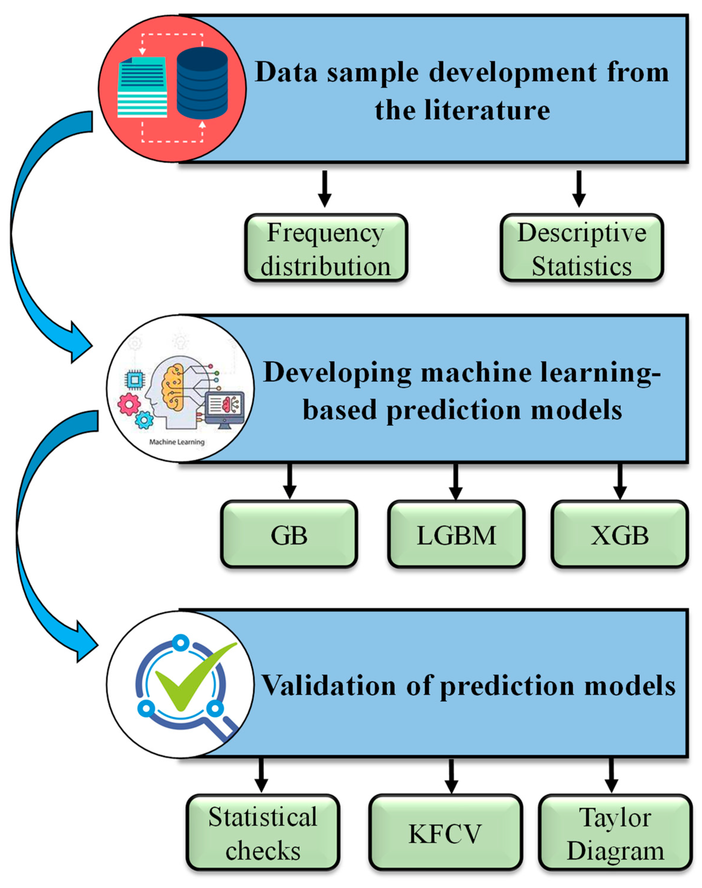
2. Research Methods
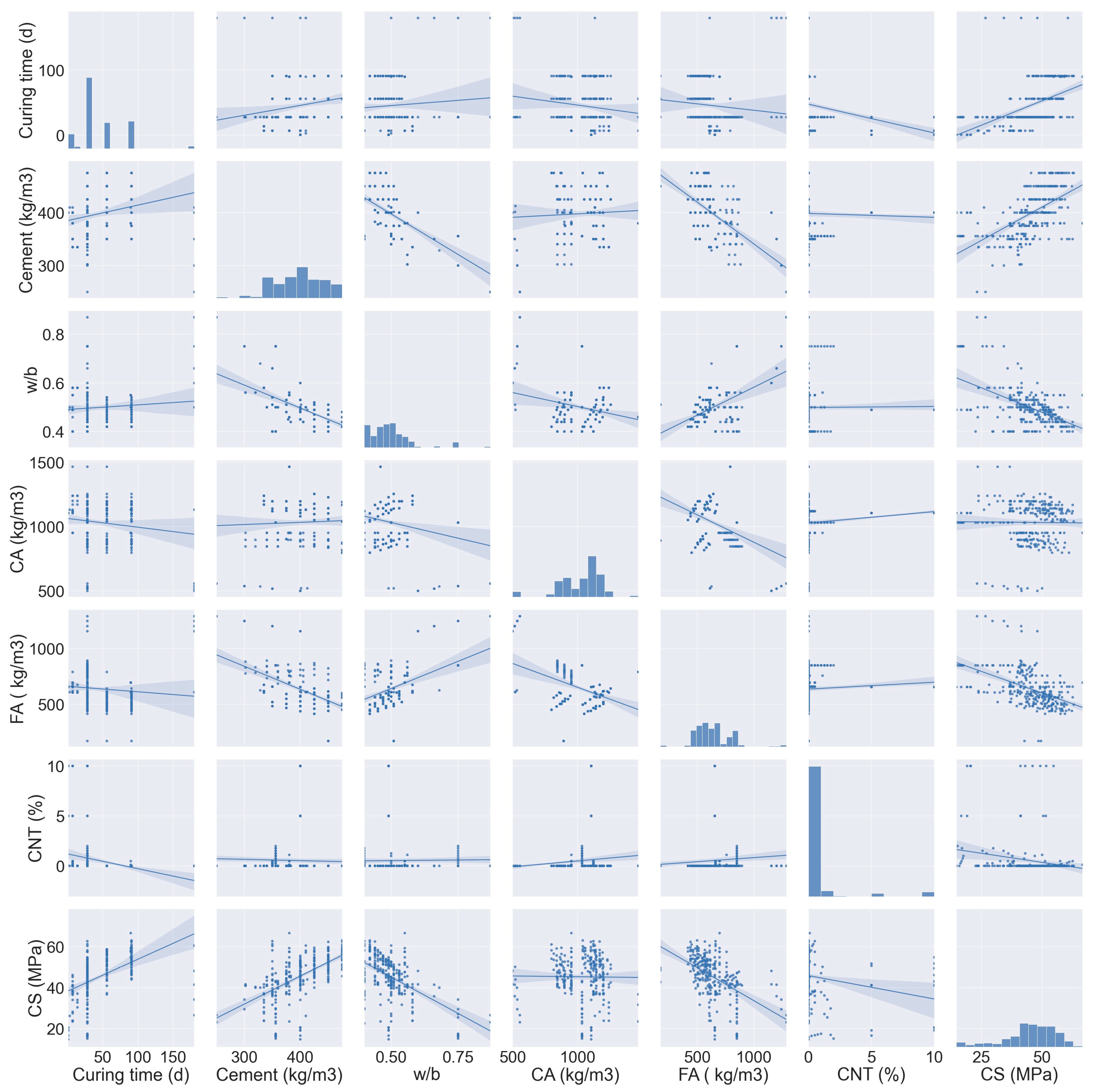
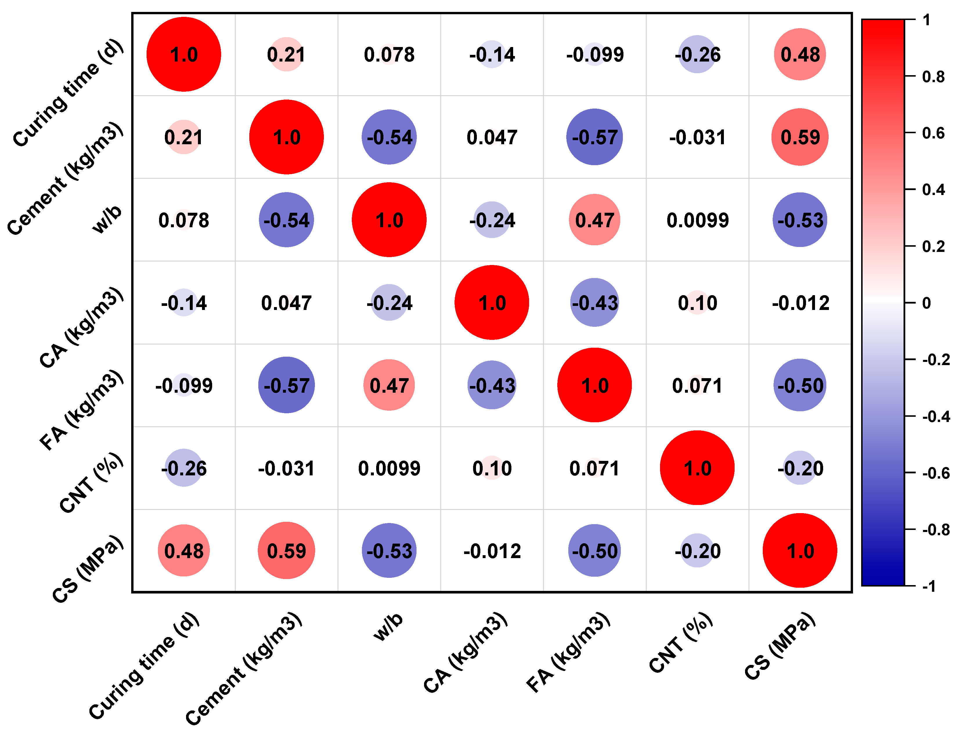
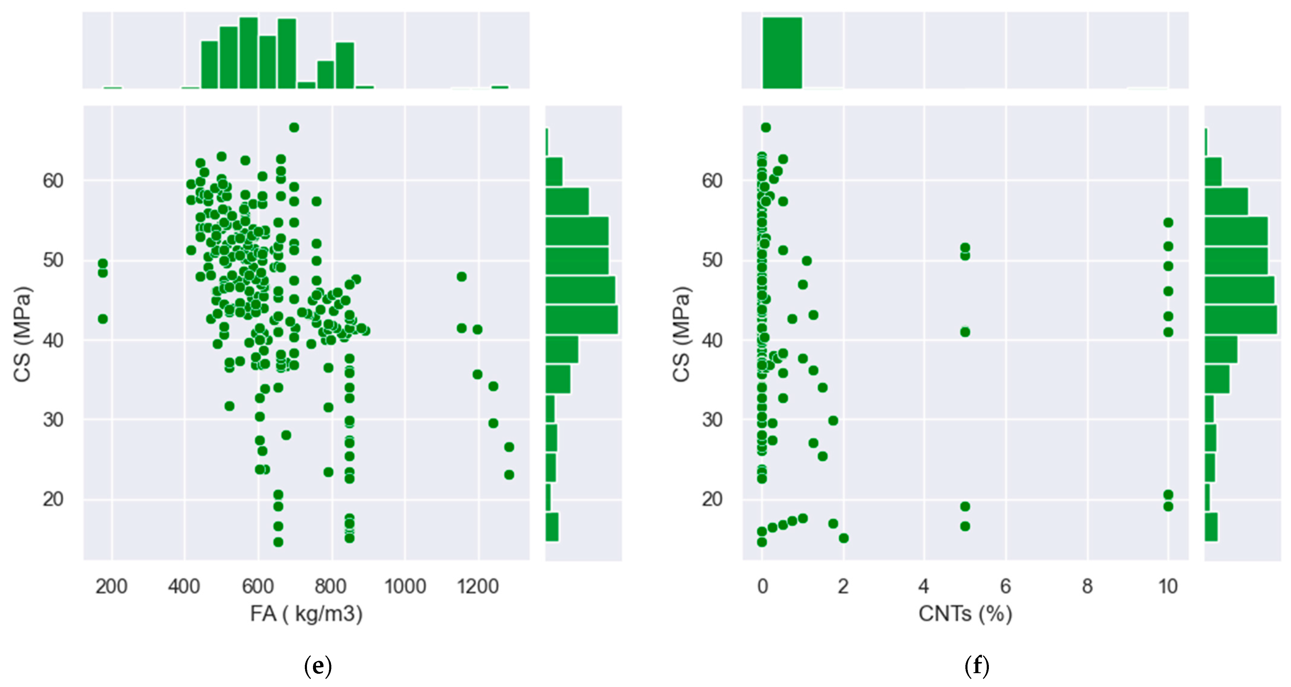
2.1. Data Description
2.2. Machine Learning Algorithms
2.2.1. Gradient Boosting
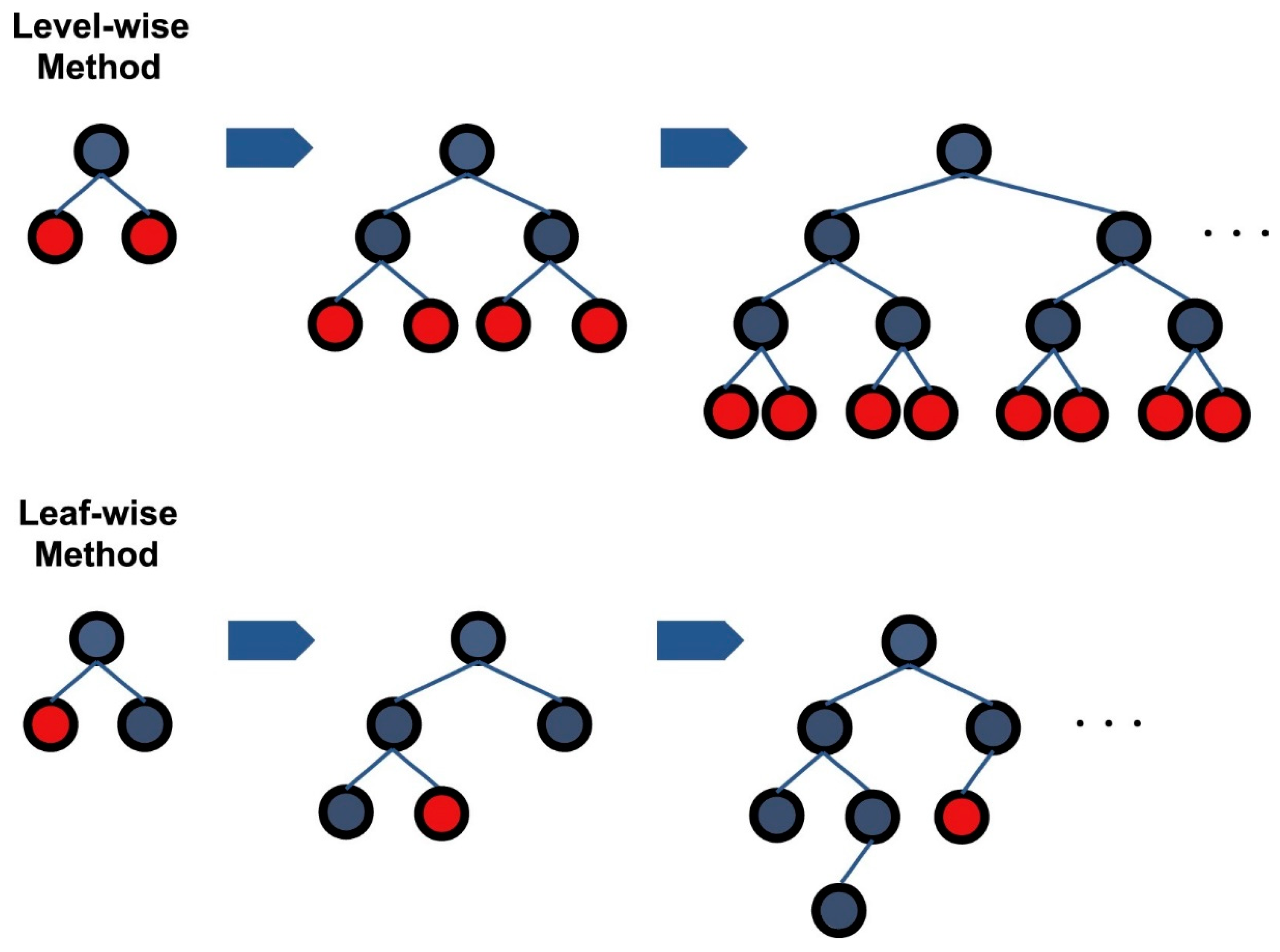
2.2.2. Light Gradient Boosting Machine
2.2.3. Extreme Gradient Boosting
2.3. Model Assessment and Validation Methods
3. Results and Discussions
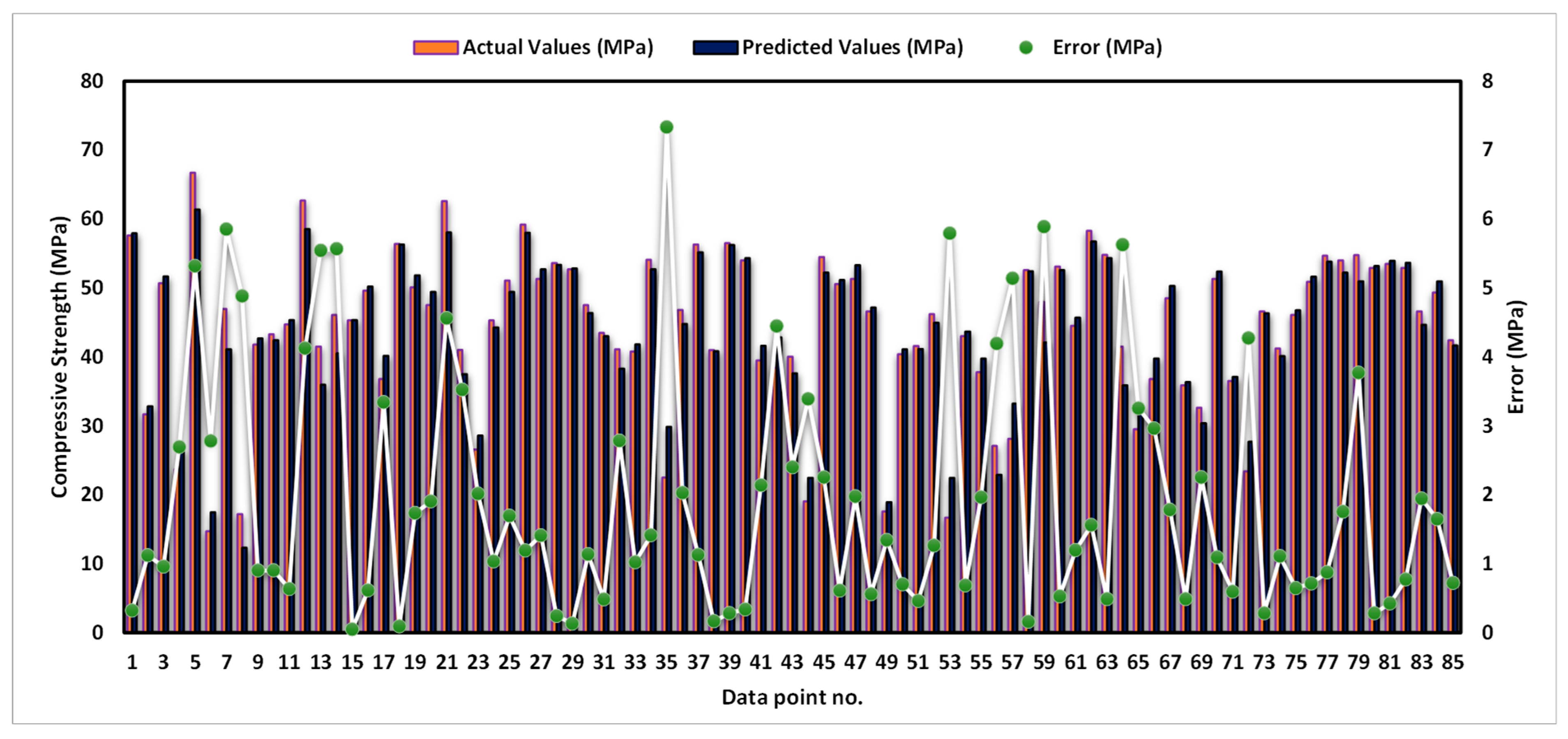
3.1. Gradient Boosting Model
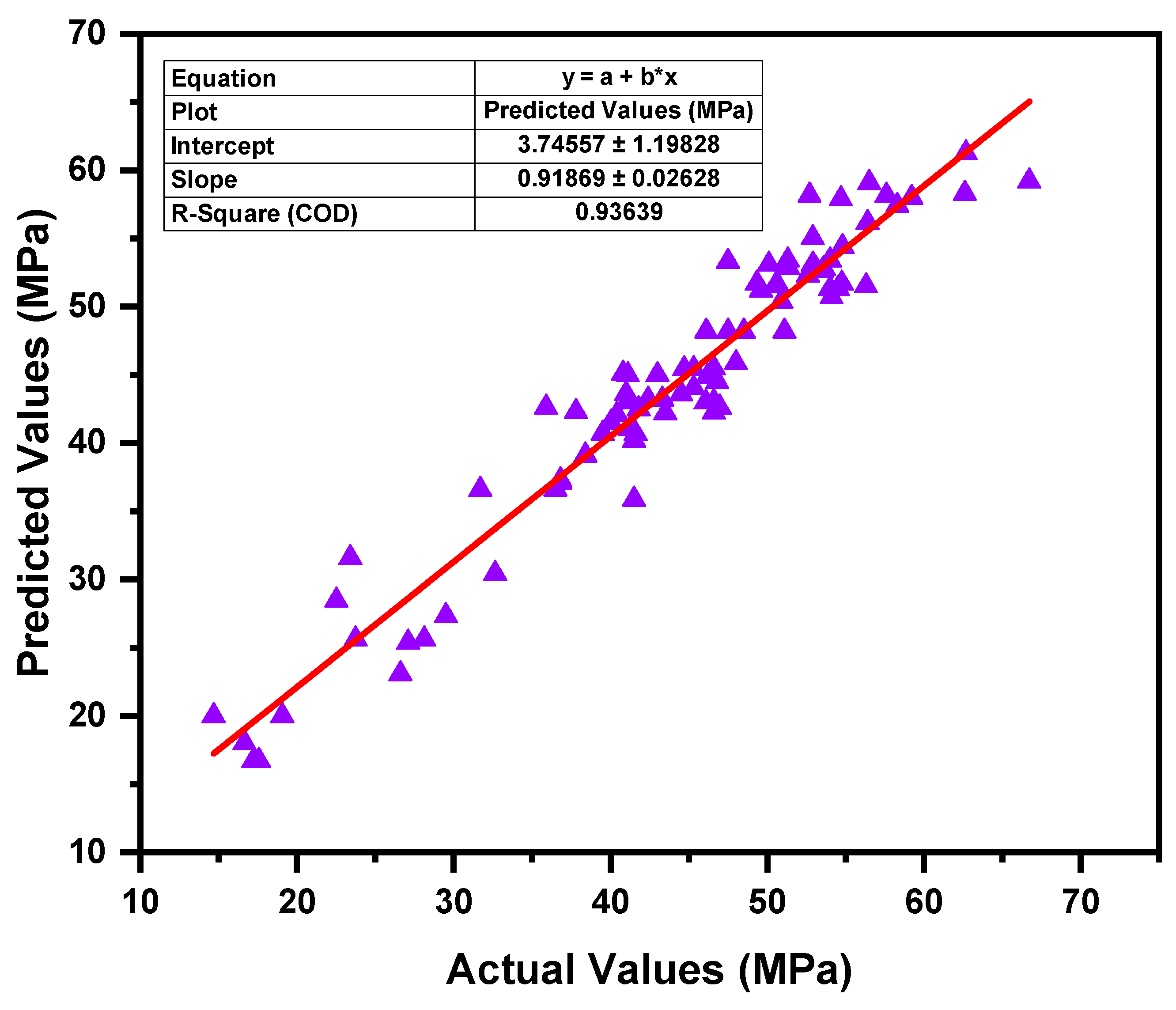
3.2. Light Gradient Boosting Machine Model
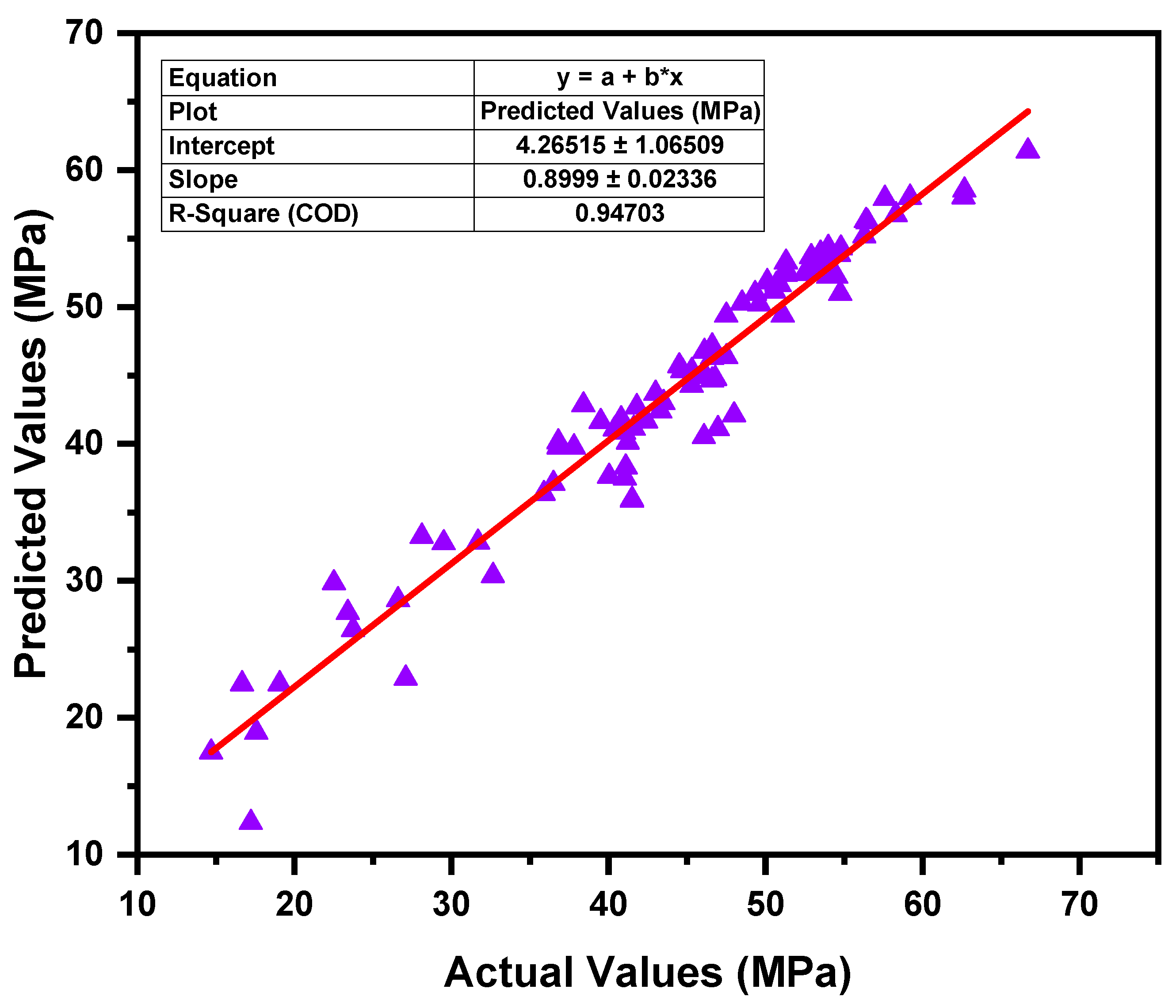
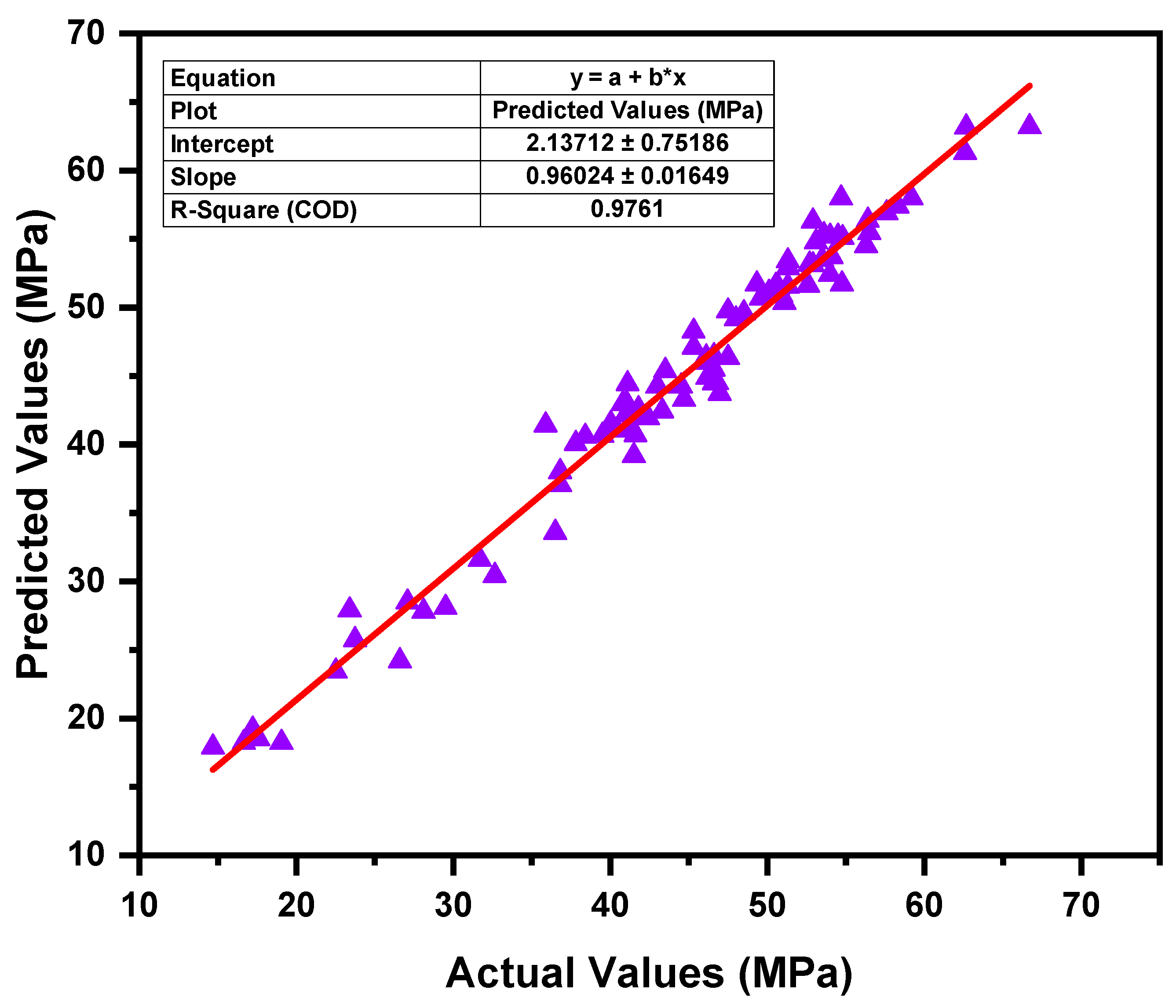
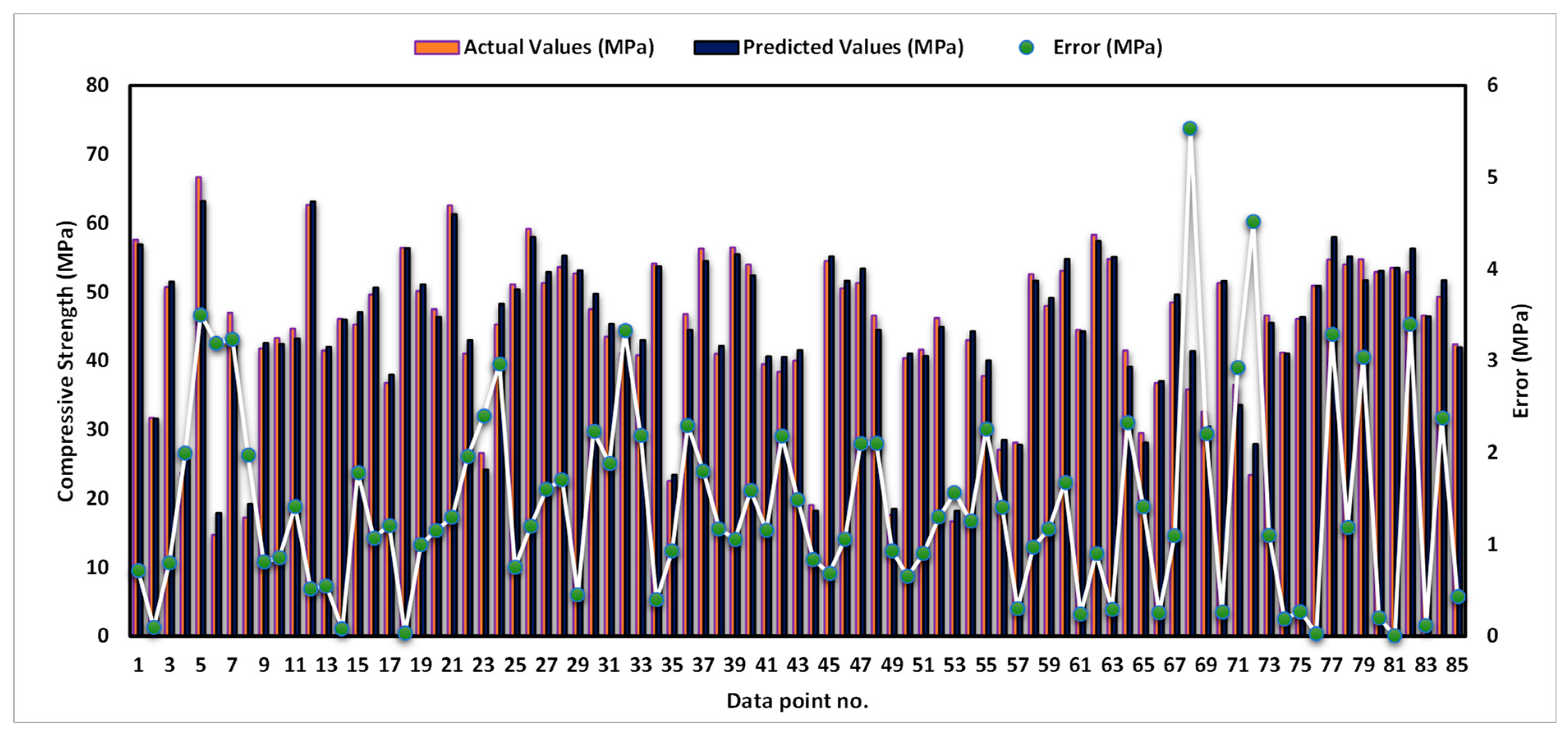
3.3. Extreme Gradient Boosting Model
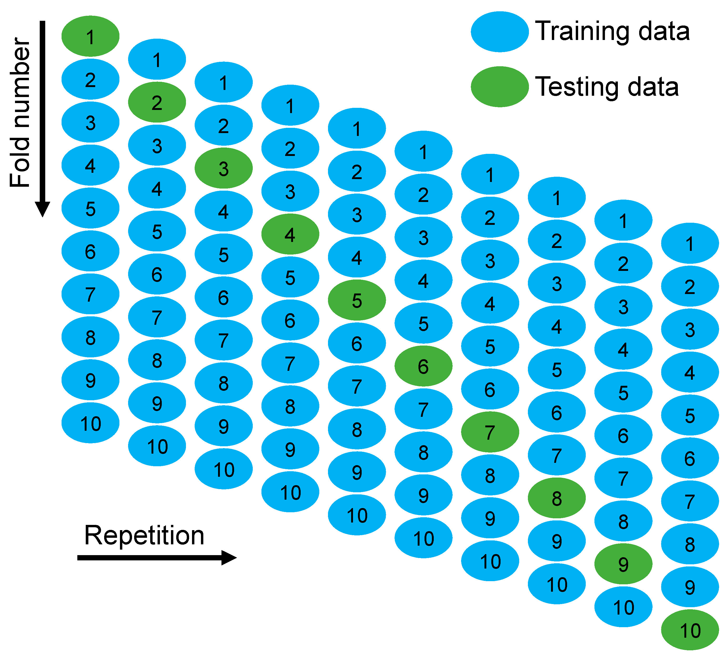
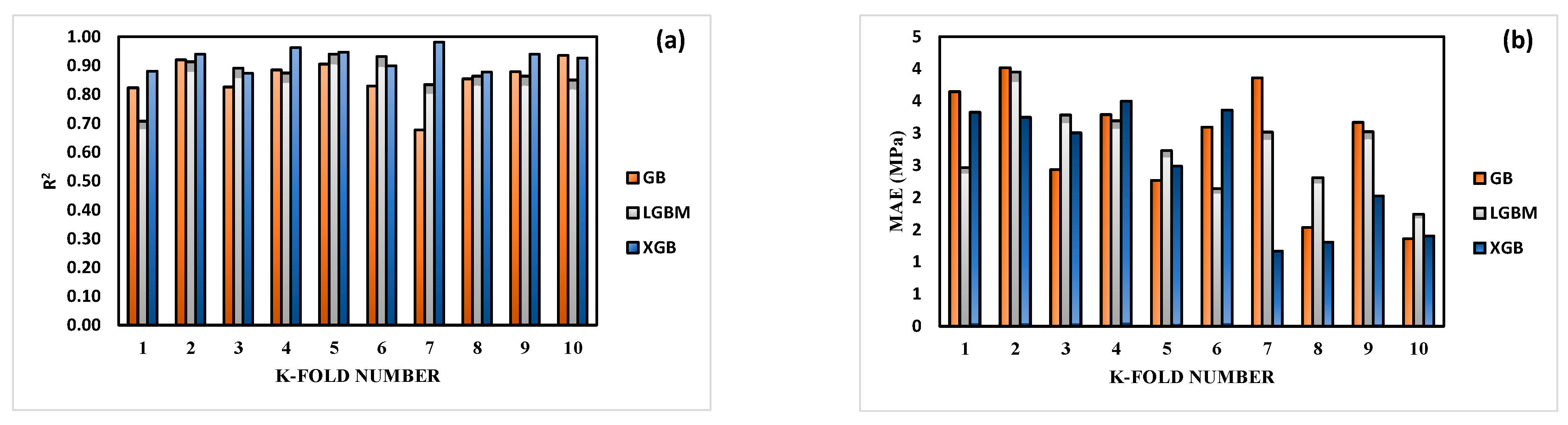
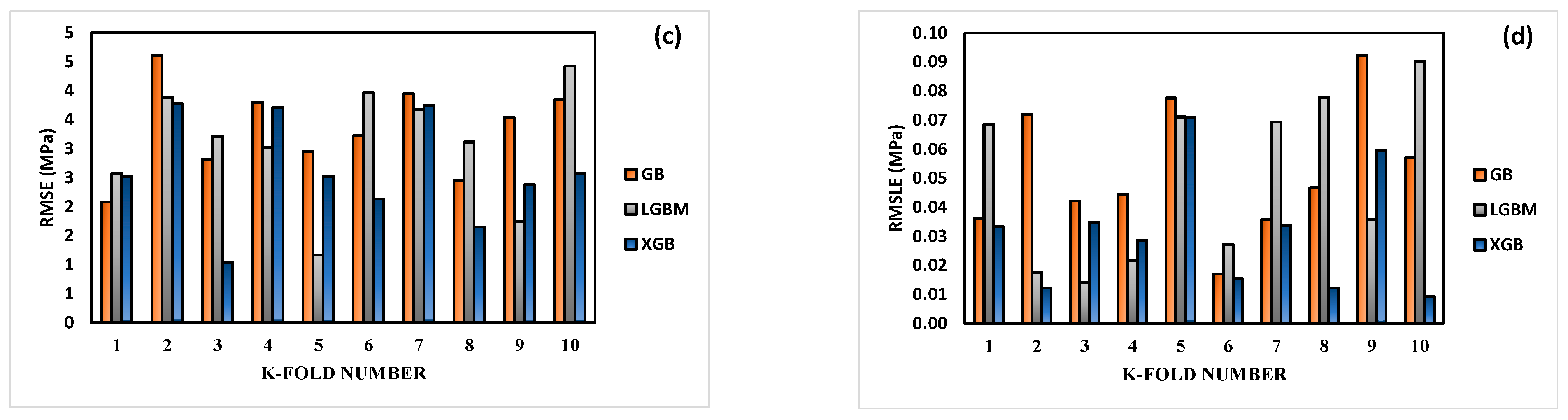
3.4. K-Fold Cross-Validation Outcomes
3.5. Statistical Performance Indicators
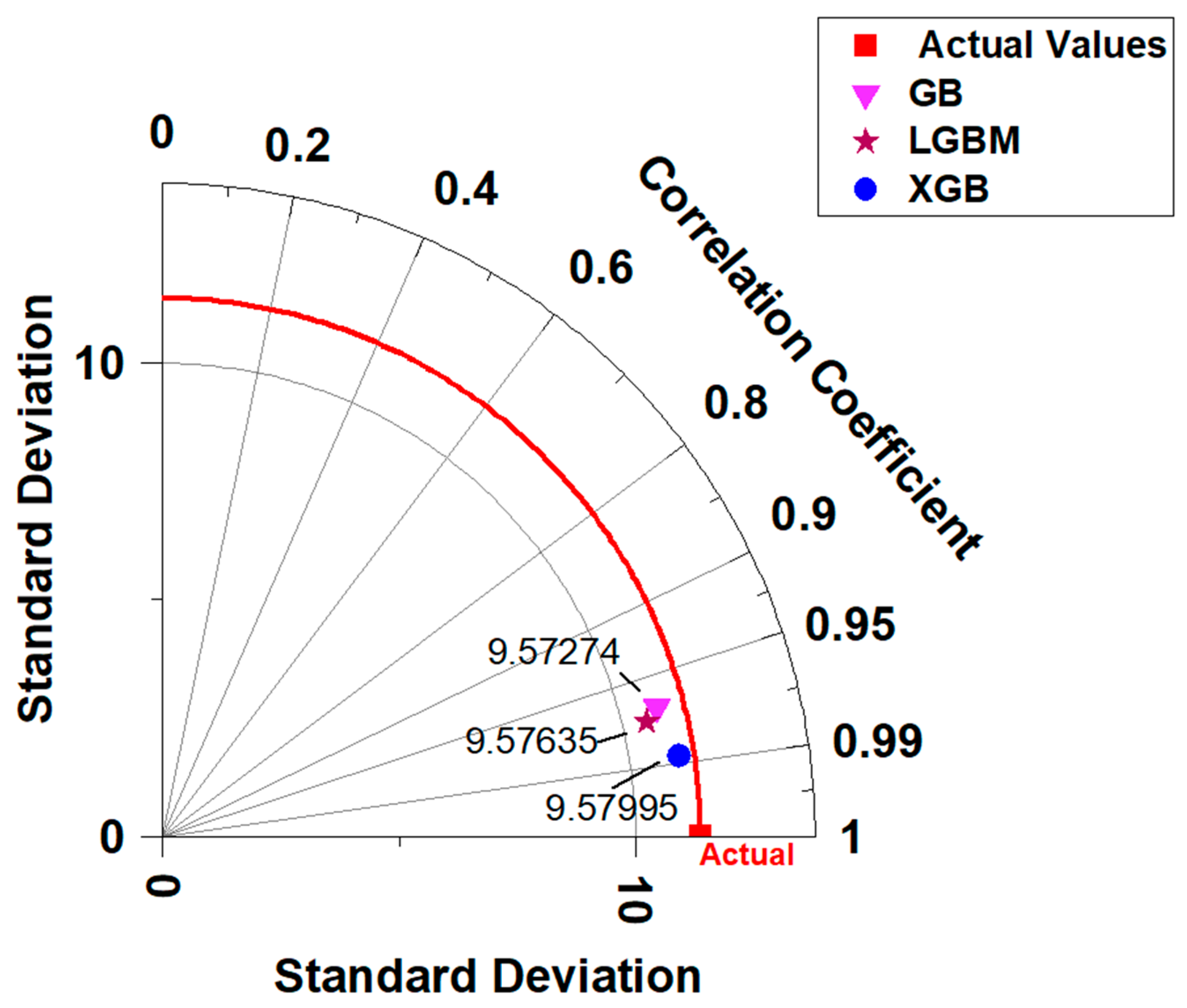
3.6. Taylor Diagrams
3.7. Interaction Analysis Outcomes
4. Discussions
5. Conclusions
- In terms of the coefficient of determination (R2), each of the three ML models, GB, LGBM, and XGB, presented convincing evidence of their accuracy. XGB surpassed the other models with the greatest R2 of 0.97, while GB and LGBM also attained R2 of 0.93 and 0.94, respectively.
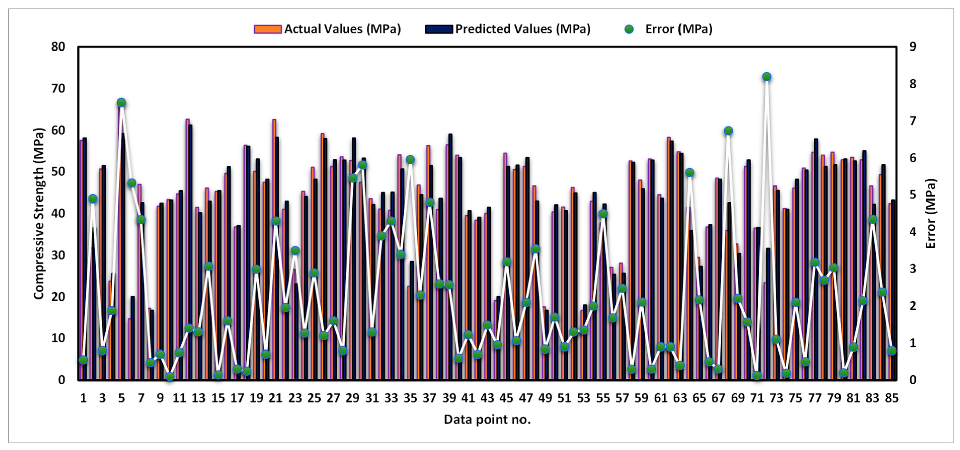
- When compared to LGBM and GB, XGB had a low error distribution, and its average error was just 1.44 MPa. This indicated that XGB’s forecasts were more accurate and had lower variability than other models’ predictions.
- During KFCV, the performance of XGB was consistently superior to that of GB and LGBM since it produced lower values for MAE, RMSE, and RMSLE. The excellence of XGB’s predictions is further shown through measurements. Similar results are also shown using statistical checks.
- The findings were verified using the Taylor diagram, which demonstrated that the values predicted by XGB were closer to the actual values than those predicted by GB and LGBM. This also demonstrated that XGB was accurate in predicting the CS of CNTs-based concrete.
- The interaction pattern indicated that at higher values of CT and cement, strength improves. To attain maximum strength, w/b, CA, and FA need to be kept low, while CNTs’ percentage needs to be kept around 1%.
Author Contributions
Funding
Data Availability Statement
Conflicts of Interest
References
- Hassan, A.; Galal, S.; Hassan, A.; Salman, A. Utilization of carbon nanotubes and steel fibers to improve the mechanical properties of concrete pavement. Beni-Suef Univ. J. Basic Appl. Sci. 2022, 11, 121. [Google Scholar] [CrossRef]
- Faraj, R.H.; Mohammed, A.A.; Omer, K.M. Self-compacting concrete composites modified with nanoparticles: A comprehensive review, analysis and modeling. J. Build. Eng. 2022, 50, 104170. [Google Scholar] [CrossRef]
- Paruthi, S.; Husain, A.; Alam, P.; Husain Khan, A.; Abul Hasan, M.; Magbool, H.M. A review on material mix proportion and strength influence parameters of geopolymer concrete: Application of ANN model for GPC strength prediction. Constr. Build. Mater. 2022, 356, 129253. [Google Scholar] [CrossRef]
- Hawreen, A.; Bogas, J.A. Creep, shrinkage and mechanical properties of concrete reinforced with different types of carbon nanotubes. Constr. Build. Mater. 2019, 198, 70–81. [Google Scholar] [CrossRef]
- Mohsen, M.O.; Al Ansari, M.S.; Taha, R.; Al Nuaimi, N.; Taqa, A.A. Carbon nanotube effect on the ductility, flexural strength, and permeability of concrete. J. Nanomater. 2019, 2019, 6490984. [Google Scholar] [CrossRef]
- Shekari, A.H.; Razzaghi, M.S. Influence of Nano Particles on Durability and Mechanical Properties of High Performance Concrete. Procedia Eng. 2011, 14, 3036–3041. [Google Scholar] [CrossRef]
- Lao, J.-C.; Xu, L.-Y.; Huang, B.-T.; Zhu, J.-X.; Khan, M.; Dai, J.-G. Utilization of sodium carbonate activator in strain-hardening ultra-high-performance geopolymer concrete (SH-UHPGC). Front. Mater. 2023, 10, 1142237. [Google Scholar] [CrossRef]
- Riaz Ahmad, M.; Khan, M.; Wang, A.; Zhang, Z.; Dai, J.-G. Alkali-activated materials partially activated using flue gas residues: An insight into reaction products. Constr. Build. Mater. 2023, 371, 130760. [Google Scholar] [CrossRef]
- Sandanayake, M.; Gunasekara, C.; Law, D.; Zhang, G.; Setunge, S.; Wanijuru, D. Sustainable criterion selection framework for green building materials—An optimisation based study of fly-ash Geopolymer concrete. Sustain. Mater. Technol. 2020, 25, e00178. [Google Scholar] [CrossRef]
- Abdalla, L.B.; Ghafor, K.; Mohammed, A. Testing and modeling the young age compressive strength for high workability concrete modified with PCE polymers. Results Mater. 2019, 1, 100004. [Google Scholar] [CrossRef]
- Lou, Y.; Khan, K.; Amin, M.N.; Ahmad, W.; Deifalla, A.F.; Ahmad, A. Performance characteristics of cementitious composites modified with silica fume: A systematic review. Case Stud. Constr. Mater. 2023, 18, e01753. [Google Scholar] [CrossRef]
- Yang, H.; Liu, L.; Yang, W.; Liu, H.; Ahmad, W.; Ahmad, A.; Aslam, F.; Joyklad, P. A comprehensive overview of geopolymer composites: A bibliometric analysis and literature review. Case Stud. Constr. Mater. 2022, 16, e00830. [Google Scholar] [CrossRef]
- Pan, Y.; Tannert, T.; Kaushik, K.; Xiong, H.; Ventura, C.E. Seismic performance of a proposed wood-concrete hybrid system for high-rise buildings. Eng. Struct. 2021, 238, 112194. [Google Scholar] [CrossRef]
- Wang, Z.; Pan, W.; Zhang, Z. High-rise modular buildings with innovative precast concrete shear walls as a lateral force resisting system. Structures 2020, 26, 39–53. [Google Scholar] [CrossRef]
- Jiao, H.; Wang, Y.; Li, L.; Arif, K.; Farooq, F.; Alaskar, A. A novel approach in forecasting compressive strength of concrete with carbon nanotubes as nanomaterials. Mater. Today Commun. 2023, 35, 106335. [Google Scholar] [CrossRef]
- De Maio, U.; Fantuzzi, N.; Greco, F.; Leonetti, L.; Pranno, A. Failure Analysis of Ultra High-Performance Fiber-Reinforced Concrete Structures Enhanced with Nanomaterials by Using a Diffuse Cohesive Interface Approach. Nanomaterials 2020, 10, 1792. [Google Scholar] [CrossRef]
- Vitharana, M.G.; Paul, S.C.; Kong, S.Y.; Babafemi, A.J.; Miah, M.J.; Panda, B. A study on strength and corrosion protection of cement mortar with the inclusion of nanomaterials. Sustain. Mater. Technol. 2020, 25, e00192. [Google Scholar] [CrossRef]
- Huseien, G.F.; Shah, K.W.; Sam, A.R.M. Sustainability of nanomaterials based self-healing concrete: An all-inclusive insight. J. Build. Eng. 2019, 23, 155–171. [Google Scholar] [CrossRef]
- Wang, Y.; Zeng, D.; Ueda, T.; Fan, Y.; Li, C.; Li, J. Beneficial effect of nanomaterials on the interfacial transition zone (ITZ) of non-dispersible underwater concrete. Constr. Build. Mater. 2021, 293, 123472. [Google Scholar] [CrossRef]
- Mohammadyan-Yasouj, S.E.; Ghaderi, A. Experimental investigation of waste glass powder, basalt fibre, and carbon nanotube on the mechanical properties of concrete. Constr. Build. Mater. 2020, 252, 119115. [Google Scholar] [CrossRef]
- Lushnikova, A.; Zaoui, A. Influence of single-walled carbon nantotubes structure and density on the ductility of cement paste. Constr. Build. Mater. 2018, 172, 86–97. [Google Scholar] [CrossRef]
- D’Alessandro, A.; Rallini, M.; Ubertini, F.; Materazzi, A.L.; Kenny, J.M. Investigations on scalable fabrication procedures for self-sensing carbon nanotube cement-matrix composites for SHM applications. Cem. Concr. Compos. 2016, 65, 200–213. [Google Scholar] [CrossRef]
- Parvaneh, V.; Khiabani, S.H. Mechanical and piezoresistive properties of self-sensing smart concretes reinforced by carbon nanotubes. Mech. Adv. Mater. Struct. 2019, 26, 993–1000. [Google Scholar] [CrossRef]
- Farooq, F.; Akbar, A.; Khushnood, R.A.; Muhammad, W.L.; Rehman, S.K.; Javed, M.F. Experimental Investigation of Hybrid Carbon Nanotubes and Graphite Nanoplatelets on Rheology, Shrinkage, Mechanical, and Microstructure of SCCM. Materials 2020, 13, 230. [Google Scholar] [CrossRef]
- Lin, W.-T. Effects of sand/aggregate ratio on strength, durability, and microstructure of self-compacting concrete. Constr. Build. Mater. 2020, 242, 118046. [Google Scholar] [CrossRef]
- Adel, H.; Ilchi Ghazaan, M.; Habibnejad Korayem, A. Chapter 9—Machine learning applications for developing sustainable construction materials. In Artificial Intelligence and Data Science in Environmental Sensing; Asadnia, M., Razmjou, A., Beheshti, A., Eds.; Academic Press: Cambridge, MA, USA, 2022; pp. 179–210. [Google Scholar]
- Huang, J.; Zhang, J.; Li, X.; Qiao, Y.; Zhang, R.; Kumar, G.S. Investigating the effects of ensemble and weight optimization approaches on neural networks’ performance to estimate the dynamic modulus of asphalt concrete. Road Mater. Pavement Des. 2023, 24, 1939–1959. [Google Scholar] [CrossRef]
- Huang, J.; Zhou, M.; Zhang, J.; Ren, J.; Vatin, N.I.; Sabri, M.M.S. Development of a new stacking model to evaluate the strength parameters of concrete samples in laboratory. Iran. J. Sci. Technol. Trans. Civ. Eng. 2022, 46, 4355–4370. [Google Scholar] [CrossRef]
- Ben Chaabene, W.; Flah, M.; Nehdi, M.L. Machine learning prediction of mechanical properties of concrete: Critical review. Constr. Build. Mater. 2020, 260, 119889. [Google Scholar] [CrossRef]
- Chen, Z.; Amin, M.N.; Iftikhar, B.; Ahmad, W.; Althoey, F.; Alsharari, F. Predictive modelling for the acid resistance of cement-based composites modified with eggshell and glass waste for sustainable and resilient building materials. J. Build. Eng. 2023, 76, 107325. [Google Scholar] [CrossRef]
- Khan, K.; Ahmad, W.; Amin, M.N.; Rafiq, M.I.; Abu Arab, A.M.; Alabdullah, I.A.; Alabduljabbar, H.; Mohamed, A. Evaluating the effectiveness of waste glass powder for the compressive strength improvement of cement mortar using experimental and machine learning methods. Heliyon 2023, 9, e16288. [Google Scholar] [CrossRef]
- Wang, N.; Xia, Z.; Amin, M.N.; Ahmad, W.; Khan, K.; Althoey, F.; Alabduljabbar, H. Sustainable strategy of eggshell waste usage in cementitious composites: An integral testing and computational study for compressive behavior in aggressive environment. Constr. Build. Mater. 2023, 386, 131536. [Google Scholar] [CrossRef]
- Taffese, W.Z.; Espinosa-Leal, L. A machine learning method for predicting the chloride migration coefficient of concrete. Constr. Build. Mater. 2022, 348, 128566. [Google Scholar] [CrossRef]
- Zheng, X.; Xie, Y.; Yang, X.; Amin, M.N.; Nazar, S.; Khan, S.A.; Althoey, F.; Deifalla, A.F. A data-driven approach to predict the compressive strength of alkali-activated materials and correlation of influencing parameters using SHapley Additive exPlanations (SHAP) analysis. J. Mater. Res. Technol. 2023, 25, 4074–4093. [Google Scholar] [CrossRef]
- Friedman, J.H. Greedy function approximation: A gradient boosting machine. Ann. Stat. 2001, 29, 1189–1232. [Google Scholar] [CrossRef]
- Dahiya, N.; Saini, B.; Chalak, H.D. Gradient boosting-based regression modelling for estimating the time period of the irregular precast concrete structural system with cross bracing. J. King Saud Univ. Eng. Sci. 2021. [Google Scholar] [CrossRef]
- Ke, G.; Meng, Q.; Finley, T.; Wang, T.; Chen, W.; Ma, W.; Ye, Q.; Liu, T.-Y. Lightgbm: A highly efficient gradient boosting decision tree. In Advances in Neural Information Processing Systems 30 (NIPS 2017), Proceedings of the 31st Conference on Neural Information Processing Systems (NIPS2017), Long Beach, CA, USA, 4–9 December 2017; Neural Information Processing Systems Foundation, Inc.: La Jolla, CA, USA, 2017. [Google Scholar]
- Fan, J.; Ma, X.; Wu, L.; Zhang, F.; Yu, X.; Zeng, W. Light Gradient Boosting Machine: An efficient soft computing model for estimating daily reference evapotranspiration with local and external meteorological data. Agric. Water Manag. 2019, 225, 105758. [Google Scholar] [CrossRef]
- Shehadeh, A.; Alshboul, O.; Al Mamlook, R.E.; Hamedat, O. Machine learning models for predicting the residual value of heavy construction equipment: An evaluation of modified decision tree, LightGBM, and XGBoost regression. Autom. Constr. 2021, 129, 103827. [Google Scholar] [CrossRef]
- Nguyen, H.; Vu, T.; Vo, T.P.; Thai, H.-T. Efficient machine learning models for prediction of concrete strengths. Constr. Build. Mater. 2021, 266, 120950. [Google Scholar] [CrossRef]
- Saud, S.; Jamil, B.; Upadhyay, Y.; Irshad, K. Performance improvement of empirical models for estimation of global solar radiation in India: A k-fold cross-validation approach. Sustain. Energy Technol. Assess. 2020, 40, 100768. [Google Scholar] [CrossRef]
- Kohavi, R. A study of cross-validation and bootstrap for accuracy estimation and model selection. In Proceedings of the International Joint Conference on Artifcial Intelligence, Montreal, QC, Canada, 20–26 August 1995; pp. 1137–1145. [Google Scholar]
- Wang, H.-L.; Yin, Z.-Y. Unconfined compressive strength of bio-cemented sand: State-of-the-art review and MEP-MC-based model development. J. Clean. Prod. 2021, 315, 128205. [Google Scholar] [CrossRef]
- Mosavi, A.; Edalatifar, M. A hybrid neuro-fuzzy algorithm for prediction of reference evapotranspiration. In Recent Advances in Technology Research and Education, Proceedings of the International Conference on Global Research and Education, Kaunas, Lithuania, 24–27 September 2018; Springer: Cham, Switzerland, 2019; pp. 235–243. [Google Scholar]
- Siahkouhi, M.; Razaqpur, G.; Hoult, N.A.; Hajmohammadian Baghban, M.; Jing, G. Utilization of carbon nanotubes (CNTs) in concrete for structural health monitoring (SHM) purposes: A review. Constr. Build. Mater. 2021, 309, 125137. [Google Scholar] [CrossRef]
- Zheng, D.; Wu, R.; Sufian, M.; Kahla, N.B.; Atig, M.; Deifalla, A.F.; Accouche, O.; Azab, M. Flexural Strength Prediction of Steel Fiber-Reinforced Concrete Using Artificial Intelligence. Materials 2022, 15, 5194. [Google Scholar] [CrossRef] [PubMed]
- Khan, K.; Ahmad, W.; Amin, M.N.; Ahmad, A.; Nazar, S.; Al-Faiad, M.A. Assessment of Artificial Intelligence Strategies to Estimate the Strength of Geopolymer Composites and Influence of Input Parameters. Polymers 2022, 14, 2509. [Google Scholar] [CrossRef]
- Khan, K.; Amin, M.N.; Sahar, U.U.; Ahmad, W.; Shah, K.; Mohamed, A. Machine learning techniques to evaluate the ultrasonic pulse velocity of hybrid fiber-reinforced concrete modified with nano-silica. Front. Mater. 2022, 9, 1098304. [Google Scholar] [CrossRef]


| Name | Abbreviation | Total Data | Mean | Standard Deviation | Sum | Minimum | Kurtosis | Skewness | Range | Median | Maximum |
|---|---|---|---|---|---|---|---|---|---|---|---|
| Curing time (d) | CT | 282 | 45.30 | 32.69 | 12,776 | 1 | 3.2 | 1.5 | 179.0 | 28 | 180 |
| Cement (kg/m3) | C | 282 | 397.82 | 45.40 | 112,186.6 | 250 | −0.3 | −0.1 | 225.0 | 400 | 475 |
| Water to binder ratio | w/b | 282 | 0.50 | 0.08 | 140.62 | 0.4 | 5.1 | 1.9 | 0.5 | 0.49 | 0.87 |
| Coarse aggregate (kg/m3) | CA | 282 | 1031.25 | 163.87 | 290,813.5 | 498 | 1.7 | −0.9 | 968.8 | 1068.75 | 1466.8 |
| Fine aggregate (kg/m3) | FA | 282 | 638.64 | 163.44 | 180,096.4 | 175.5 | 3.2 | 1.2 | 1109.5 | 608.375 | 1285 |
| Carbon nanotubes (%) | CNT | 282 | 0.51 | 1.89 | 145.21 | 0 | 18.4 | 4.4 | 10.0 | 0 | 10 |
| Compressive strength (MPa) | CS | 282 | 45.14 | 10.57 | 12,730.26 | 14.7 | 0.6 | −0.9 | 52.0 | 46.5 | 66.7 |
| K-Fold | GB Model | LGBM Model | XGB Model | |||||||||
|---|---|---|---|---|---|---|---|---|---|---|---|---|
| R2 | MAE (MPa) | RMSE (MPa) | RMSLE (MPa) | R2 | MAE (MPa) | RMSE (MPa) | RMSLE (MPa) | R2 | MAE (MPa) | RMSE (MPa) | RMSLE (MPa) | |
| 1 | 0.82 | 3.65 | 2.08 | 0.036 | 0.71 | 2.47 | 2.57 | 0.068 | 0.88 | 3.33 | 2.52 | 0.033 |
| 2 | 0.92 | 4.02 | 4.60 | 0.072 | 0.91 | 3.95 | 3.89 | 0.017 | 0.94 | 3.25 | 3.78 | 0.012 |
| 3 | 0.83 | 2.43 | 2.82 | 0.042 | 0.89 | 3.28 | 3.21 | 0.014 | 0.87 | 3.01 | 1.04 | 0.035 |
| 4 | 0.89 | 3.29 | 3.80 | 0.044 | 0.87 | 3.19 | 3.02 | 0.022 | 0.96 | 3.50 | 3.71 | 0.029 |
| 5 | 0.91 | 2.27 | 2.96 | 0.078 | 0.94 | 2.73 | 1.16 | 0.071 | 0.95 | 2.49 | 2.52 | 0.071 |
| 6 | 0.83 | 3.09 | 3.23 | 0.017 | 0.93 | 2.14 | 3.96 | 0.027 | 0.90 | 3.36 | 2.13 | 0.015 |
| 7 | 0.68 | 3.86 | 3.95 | 0.036 | 0.83 | 3.02 | 3.68 | 0.069 | 0.98 | 1.17 | 3.75 | 0.034 |
| 8 | 0.85 | 1.53 | 2.46 | 0.047 | 0.86 | 2.31 | 3.11 | 0.078 | 0.88 | 1.31 | 1.65 | 0.012 |
| 9 | 0.88 | 3.17 | 3.53 | 0.092 | 0.86 | 3.03 | 1.74 | 0.036 | 0.94 | 2.03 | 2.38 | 0.060 |
| 10 | 0.94 | 1.36 | 3.84 | 0.057 | 0.85 | 1.74 | 4.42 | 0.090 | 0.93 | 1.41 | 2.57 | 0.009 |
| Max | 0.94 | 4.02 | 4.60 | 0.092 | 0.94 | 3.95 | 4.42 | 0.090 | 0.98 | 3.50 | 3.78 | 0.071 |
| Min | 0.68 | 1.36 | 2.08 | 0.017 | 0.71 | 1.74 | 1.16 | 0.014 | 0.87 | 1.17 | 1.04 | 0.009 |
| Mean | 0.85 | 2.87 | 3.33 | 0.052 | 0.87 | 2.79 | 3.08 | 0.049 | 0.92 | 2.48 | 2.60 | 0.031 |
| Technique | GB | LGBM | XGB |
|---|---|---|---|
| MAE (MPa) | 2.195 | 2.0 | 1.445 |
| MAPE | 5.70% | 5.70% | 3.80% |
| RMSE (MPa) | 2.863 | 2.844 | 1.798 |
| RMSLE (MPa) | 0.065 | 0.064 | 0.041 |
| Ref. | Material Studied | Properties Predicted | ML Techniques Employed | Optimum ML Model Noted | R2 of the Best ML Model |
|---|---|---|---|---|---|
| Current study | CNTs-based concrete | CS | GB, LGBM, and XGB | XGB | 0.97 |
| [32] | Eggshell-based cement mortar | Reduction in CS after acid attack | GB, AdaBoost, and XGB | XGB | 0.94 |
| [46] | Steel fibre reinforced concrete | Flexural strength | GB, random forest, and XGB | XGB | 0.94 |
| [47] | Geopolymer concrete | CS | Support vector machine, GB, and XGB | XGB | 0.98 |
| [48] | Nano-silica modified concrete | Ultrasonic pulse velocity | GB, AdaBoost, and XGB | XGB | 0.90 |
Disclaimer/Publisher’s Note: The statements, opinions and data contained in all publications are solely those of the individual author(s) and contributor(s) and not of MDPI and/or the editor(s). MDPI and/or the editor(s) disclaim responsibility for any injury to people or property resulting from any ideas, methods, instructions or products referred to in the content. |
© 2024 by the authors. Licensee MDPI, Basel, Switzerland. This article is an open access article distributed under the terms and conditions of the Creative Commons Attribution (CC BY) license (https://creativecommons.org/licenses/by/4.0/).
Share and Cite
Zhu, F.; Wu, X.; Lu, Y.; Huang, J. Strength Estimation and Feature Interaction of Carbon Nanotubes-Modified Concrete Using Artificial Intelligence-Based Boosting Ensembles. Buildings 2024, 14, 134. https://0-doi-org.brum.beds.ac.uk/10.3390/buildings14010134
Zhu F, Wu X, Lu Y, Huang J. Strength Estimation and Feature Interaction of Carbon Nanotubes-Modified Concrete Using Artificial Intelligence-Based Boosting Ensembles. Buildings. 2024; 14(1):134. https://0-doi-org.brum.beds.ac.uk/10.3390/buildings14010134
Chicago/Turabian StyleZhu, Fei, Xiangping Wu, Yijun Lu, and Jiandong Huang. 2024. "Strength Estimation and Feature Interaction of Carbon Nanotubes-Modified Concrete Using Artificial Intelligence-Based Boosting Ensembles" Buildings 14, no. 1: 134. https://0-doi-org.brum.beds.ac.uk/10.3390/buildings14010134