Analytical Solution for the Ultimate Compression Capacity of Unbonded Steel-Mesh-Reinforced Rubber Bearings

Abstract

Unbonded steel-mesh-reinforced rubber bearings (USRBs) have been proposed as an alternative isolation bearing for small-to-medium-span highway bridges. It replaces the steel plate reinforcement of common unbonded laminated rubber bearings (ULNR) with special steel wire meshes, resulting in improved lateral properties and seismic performance. However, the impact of this novel steel wire mesh reinforcement on the ultimate compression capacity of USRB has not been studied. To this end, theoretical and experimental analysis of the ultimate compression capacity of USRBs were carried out. The closed-form analytical solution of the ultimate compression capacity of USRBs was derived from a simplified USRB model employing elasticity theory. A parametric study was conducted considering the geometric and material properties. Ultimate compression tests were conducted on 19 USRB specimens to further calibrate the analytical solution, considering the influence of the number of reinforcement layers. An efficient solution for USRBs’ ultimate compression capacity was obtained via multilinear regression of the calibrated analytical results. The efficient solution can simplify the estimation of USRBs’ ultimate compression capacity while maintaining the same accuracy as the calibrated solution. Based on the efficient solution, the design process of a USRB with a specific ultimate compression capacity was illustrated.

1. Introduction

The unbonded laminated rubber bearing (ULNR) has been widely used in short-to-medium-span highway bridges in China for decades due to its cost-effectiveness, ease of manufacturing, and seismic isolation capacity [1,2,3,4]. The ULNR is laminated with natural rubber layers and rigid steel plate reinforcement. The term “unbonded” refers to the bearings being directly placed on top of the piers and having no bonding with the structures. This boundary condition helps reduce bearing costs and construction labor. However, it also introduces the problem of bearing sliding when shear deformation exceeds a certain threshold. This sliding behavior, characterized by zero yielding stiffness, cannot be controlled once it is initiated [5]. Moreover, the deformation threshold for ULNRs is relatively limited because only the rubber layer can provide lateral deformation, while the rigid steel plate reinforcement cannot contribute to it. During the 2008 Mw 7.9 Wenchuan earthquake, excessive sliding deformation of ULNRs was widely witnessed in highway bridges, which led to girder dislocation and even span collapse [6,7]. To address this problem, we came up with using the flexible steel woven wire mesh as an alternative reinforcement for the ULNR to increase its lateral deformation threshold before sliding [8,9,10]. We named the bearing the unbonded steel-mesh-reinforced rubber bearing (USRB). The flexible reinforcement enables USRB to display rolling-like deformation under lateral loading. Specifically, the vertical surface of the bearing will incline and bend towards the horizontal plane, while the top and bottom surfaces will roll off from the horizontal plane. Owing to the characteristic rolling deformation, the reinforcement layers can participate in the deforming, thereby increasing the lateral deformation capacity. Additionally, this rolling behavior can reduce the lateral stiffness of the bearing. Lateral cyclic loading tests have confirmed that the rolling of USRBs is stable and USRB can provide a larger lateral deformation capacity compared to ULNR [8,9]. Shaking table tests have been carried out in Tongji University to compare the seismic performance of USRBs and ULNRs in a two-span continuous girder bridge [9,10]. The results show that USRBs, with their reduced lateral stiffness, can mitigate more lateral force transmitted from superstructure to substructure compared to ULNR-isolated systems. Meanwhile, USRBs exhibited the ability to sustain larger structural relative displacements during strong ground motions.

Similar to the USRB, the Fiber-Reinforced Elastomeric Isolator (FREI) also applies flexible reinforcement, such as glass fiber sheets, carbon fiber sheets, and carbon fiber reinforced polymer plates [11,12,13,14,15,16]. It can also display rolling deformation. However, FREIs are manufactured through the cold vulcanization process, where a curing rubber adhesive is used to bond the rubber and reinforcement. The cold bonding of FREIs would result in delamination damage between rubber and fiber reinforcement under large shear deformation. In contrast, the USRB employs hot vulcanization to guarantee a strong bond between the steel mesh and rubber layers. Additionally, the apertures presented in the steel mesh increase the adhesive area, further strengthening the bond.

During severe earthquakes such as the 1985 Nahanni, 1994 Northridge, and 1995 Kobe events, it has been observed that the vertical ground motion may significantly exceed the horizontal ground motion [17]. This elevated vertical motion can greatly amplify the axial forces experienced by the bearings and substructures [18]. As a result, the most recent code in China [19] has increased the vertical design load of isolation bearings by a factor of three. Under these circumstances, FREIs may not provide satisfactory vertical compression capacity due to unreliable bonding between fiber reinforcement and rubber, as indicated by previous research on their ultimate compression capabilities (e.g., a maximum capacity of 16 MPa for carbon-fiber-reinforced bearing) [20,21,22]. In contrast, USRBs exhibit an average ultimate compression capacity of 52 MPa during the prototype testing stage [9]. This higher capacity of USRBs makes them a promising solution for bearings with flexible reinforcement for meeting the increased vertical design load requirements mandated by the current code. However, a thorough investigation on the ultimate compression capacity of USRBs has not been conducted. In this regard, this paper presents the analytical and experimental studies conducted to assess the ultimate compression capacity of USRBs.

Previous research on the vertical mechanics of bearings with flexible reinforcement were mainly focused on the vertical stiffness or the effect of vertical load on lateral performance [23]. Based on the study of bonded rubber blocks’ compression [24,25], Kelly [26] first analyzed the vertical stiffness of multilayered rubber bearings with rigid reinforcement. Various bearing cross-section shapes were examined, including circular, square, and annular. Then, Kelly [11] developed the approach for infinitely long-strip-fiber-reinforced bearings considering the flexibility of fiber reinforcements. The developed approach was later applied by Tsai and Kelly [27,28,29] to predict the compression stiffness of rectangular and circular fiber-reinforced bearings. Kelly and Takhirov [30] further promoted the analytical method to include the influence of rubber compressibility for the fiber-reinforced bearings with large shape factors. Over the last decade, the approach has been expanded to include bearings with a general cross-sectional shape [31] or with zero Poisson’s ratio reinforcements [32]. However, despite the systematic research conducted on the vertical stiffness, ultimate compression capacity as one important factor of the vertical mechanics of bearings also needs to be analyzed. Our research aims to fill in this gap by developing a theoretical solution for USRBs’ compression capacity to guide their further optimal design.

The prototype testing [9] showed that the steel woven wire mesh reinforcement of USRBs experienced tensile failure under ultimate compression loading. This indicates that the ultimate compression capacity of USRBs can be obtained by analyzing the internal force of the reinforcement, which forms the basis of this study.

This paper presents an analytical solution for the ultimate compression capacity of rectangular unbonded steel-mesh-reinforced rubber bearings. A parametric study was then conducted to investigate the relative importance of various geometric parameters and material properties on compression capacity. To include the effect of the number of reinforcement layers, the analytical solution was further calibrated with ultimate compression test results of 19 USRB specimens. To facilitate engineering application, an efficient solution for the ultimate compression capacity of USRBs was obtained via multiple linear regression. Based on the above research, a preliminary design process of USRBs to meet a specific ultimate compression capacity requirement was provided. This study fills in the gap of analytical analysis on the ultimate behavior of USRBs under compression, and provides a basis for enhancing existing USRBs’ compression capacity, which play an important role in ensuring the seismic resilience of highway bridges.

2. Mechanics of Rectangular USRBs under Compression

2.1. Hypothesis

Unbonded steel-mesh-reinforced rubber bearings (USRBs) consist of alternating rubber layers and steel mesh reinforcement. All rubber layers in the bearing are assumed to have the same deformation and stress distribution under vertical compression loading. To simplify the analysis, only one rubber layer is studied, as shown in Figure 1. The steel mesh reinforcement is treated as a continuous solid layer with an equivalent thickness to maintain the same tensile stress in the discrete wire mesh. The value of the equivalent thickness will be discussed in Section 2.3. All materials, including rubber and steel reinforcement, are regarded as linearly elastic so that the linear elastic theory can be applied. The theoretical analysis is based on the following assumptions [11]: (a) the vertical line before loading becomes a parabola after loading; (b) the horizontal plane section before loading remains plane after loading; and (c) the stress state in the rubber is dominated by internal pressure, p.

2.2. Equilibrium in the Rubber Layer

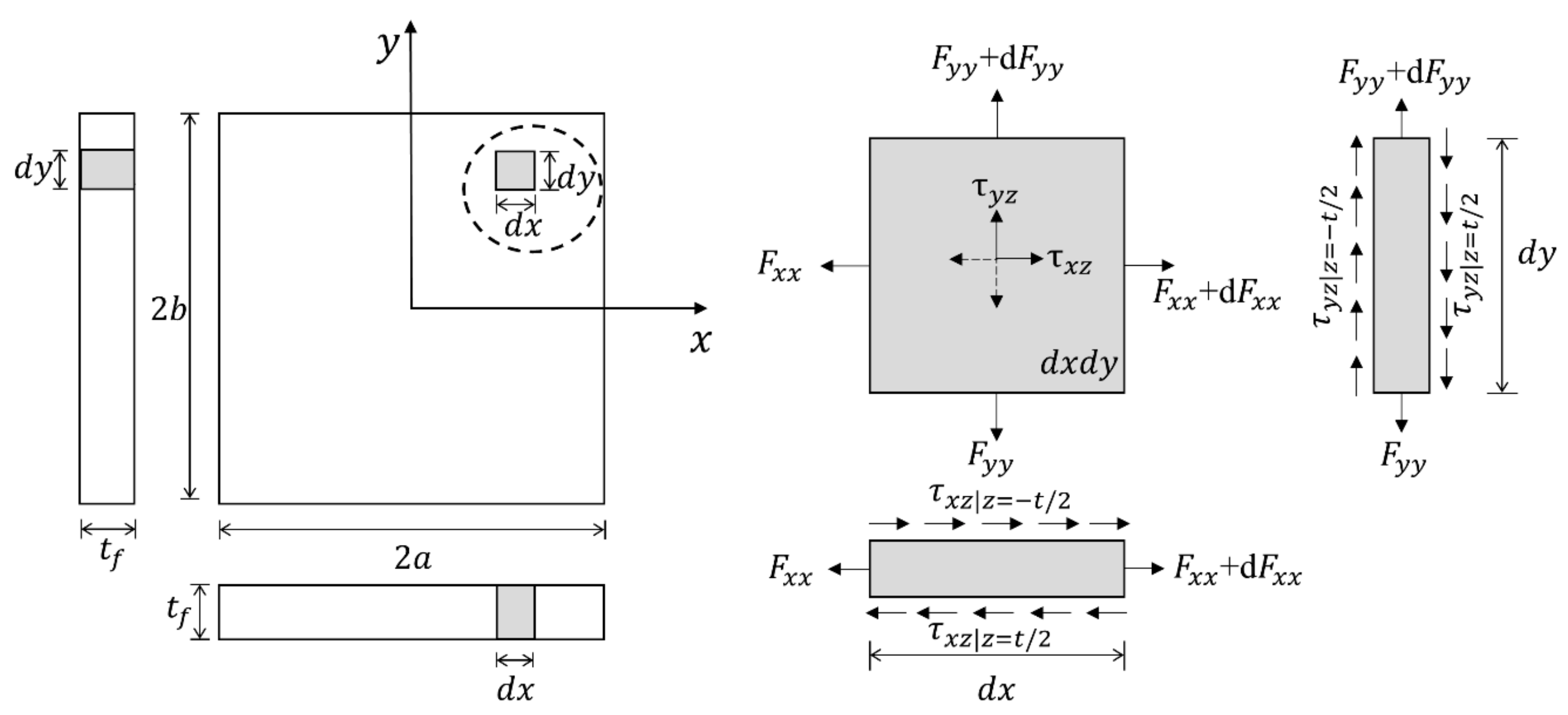
The single rubber layer reinforced by two steel mesh reinforcements is shown in Figure 1a. The rubber layer has a thickness of t, a width of 2a, and a length of 2b, where $a\le b$. It is firmly bonded with the top and bottom steel reinforcement layers, each with an equivalent thickness of t_s. The Cartesian coordinate system (x, y, z) is located at the center of the rubber layer. A vertical compressive load P is applied to the whole pad along the z-axis. Under load P, the rubber layer bulges laterally with the extension of the flexible steel mesh reinforcement, as illustrated in Figure 1b,c. The displacement of any one point (x, y, z) in the rubber layer along the x-, y-, and z-axis is denoted as u(x, y, z), v(x, y, z), and w(x, y, z), respectively, and is expressed in the form of Equation (1). According to assumption (a), the side profile of the rubber layer should be quadratic along z. The u₀(x, y) and v₀(x, y) denote the maximum bulging deformation of rubber along the x- and y-axis, respectively, compared with the reinforcement. The u₁(x, y) and v₁(x, y) represent the tensile deformation of the reinforcement along the x- and y-axis, respectively, which is constant throughout the thickness. According to assumption (b) that the horizontal plane remains plane, w(x, y, z) can be simplified to w(z). $\Delta t$ is the compression deformation of the rubber layer under vertical load P.

$$\left\{\begin{array}{l}u(x,y,z)=u_0(x,y)(1-\frac{4z^2}{t^2})+u_1(x,y)\\ v(x,y,z)=v_0(x,y)(1-\frac{4z^2}{t^2})+v_1(x,y)\\ w(x,y,z)=w(z)\end{array}\right.$$

(1)

The equilibrium equations for the stress in the rubber layer are shown in Equation (2), where ${\tau }_{xy}={\tau }_{yx}$, ${\tau }_{yz}={\tau }_{zy}$, and ${\tau }_{xz}={\tau }_{zx}$, according to the reciprocal theorem of shear stress.

$$\begin{array}{l}{\sigma }_{xx,x}+{\tau }_{yx,y}+{\tau }_{zx,z}=0\\ {\tau }_{xy,x}+{\sigma }_{yy,y}+{\tau }_{zy,z}=0\\ {\tau }_{xz,x}+{\tau }_{yz,y}+{\sigma }_{zz,z}=0\end{array}$$

(2)

As stated in assumption (c), the stress state of rubber is dominated by the internal pressure p, such that the difference between the normal stress $\sigma$ and $-p$ is of the order $p{t}^2/a^2$ [27]. And, the shear stresses ${\tau }_{xz},{\tau }_{yz}$ generated by the reinforcement are considered to be of order $pt/a$, while the in-plane shear stress ${\tau }_{xy}$ is of order $p{t}^2/a^2$ [27]. Considering the rubber layer thickness t is one to two orders of magnitude smaller than the width of rubber layer 2a, the stress in the rubber can be approximated by

$$\begin{array}{l}{\sigma }_{xx}\approx {\sigma }_{yy}\approx {\sigma }_{zz}\approx -p\\ {\tau }_{xy}=0\end{array}$$

(3)

Then, Equation (2) can be reduced to

$$\begin{array}{l}{p}_{,x}={\tau }_{xz,z}\\ p_{,y}={\tau }_{yz,z}\end{array}$$

(4)

Assuming that the rubber is compressible and has a bulk modulus of K, the volumetric strain of the rubber layer under the stress state of Equation (4) can be determined by

$${\epsilon }_{xx}+{\epsilon }_{yy}+{\epsilon }_{zz}=-\frac{p}{K}$$

(5)

where the normal strain is calculated by ${\epsilon }_{xx}=u_{,x}$, ${\epsilon }_{yy}=v_{,y}$, and ${\epsilon }_{zz}=w_{,z}$, according to the strain-displacement equations of elasticity. Equation (5) is also the strain compatibility equation of the rubber layer and will be applied to solve the stress solution of p in this study.

Substituting Equation (1) into Equation (5) and integrating from $z=-t/2$ to $z=t/2$, we can calculate the strain compatibility equation in terms of displacement:

$$\frac{2}{3}(u_{0,x}+v_{0,y})+u_{1,x}+v_{1,y}={\epsilon }_c-\frac{p}{K}$$

(6)

where ${\epsilon }_c$ is the vertical compression strain of the rubber layer and is defined in Equation (7). It is noted that ${\epsilon }_c$ is positive in the case of compression.

$${\epsilon }_c=\frac{\Delta t}{t}=-\left[\frac{w(\frac{t}{2})-w(-\frac{t}{2})}{t}\right]$$

(7)

Due to the linearly elastic behavior of rubber, the shear stress $\tau$ in the rubber layer satisfies the following constitutive law:

$$\begin{array}{l}{\tau }_{xz}=G{\gamma }_{xz}\\ {\tau }_{yz}=G{\gamma }_{yz}\end{array}$$

(8)

where G is the shear modulus of rubber, and the shear strain $\gamma$ can be determined by the following strain-displacement equations:

$$\begin{array}{l}{\gamma }_{xz}=u_{,z}+w_{,x}=-8u_0\frac{z}{t^2}\\ {\gamma }_{yz}=v_{,z}+w_{,y}=-8v_0\frac{z}{t^2}\end{array}$$

(9)

Substituting Equation (9) into Equation (8), the shear stress $\tau$ in the rubber can be expressed in terms of displacement:

$$\begin{array}{l}{\tau }_{xz}=-8G{u}_0\frac{z}{t^2}\\ {\tau }_{yz}=-8G{v}_0\frac{z}{t^2}\end{array}$$

(10)

Considering the relationship between p and shear stress $\tau$ in Equation (4), the above equation is substituted into Equation (4) to obtain the expression of internal pressure p in terms of displacement.

$$\begin{array}{l}{p}_{,x}=-\frac{8G{u}_0}{t^2}\\ p_{,y}=-\frac{8G{v}_0}{t^2}\end{array}$$

(11)

Differentiating Equation (11) with respect to x and y, respectively, leads to

$$\begin{array}{l}{u}_{0,x}=-\frac{t^2}{8G}{p}_{,xx}\\ v_{0,y}=-\frac{t^2}{8G}{p}_{,yy}\end{array}$$

(12)

2.3. Equilibrium in The Reinforcement Layer

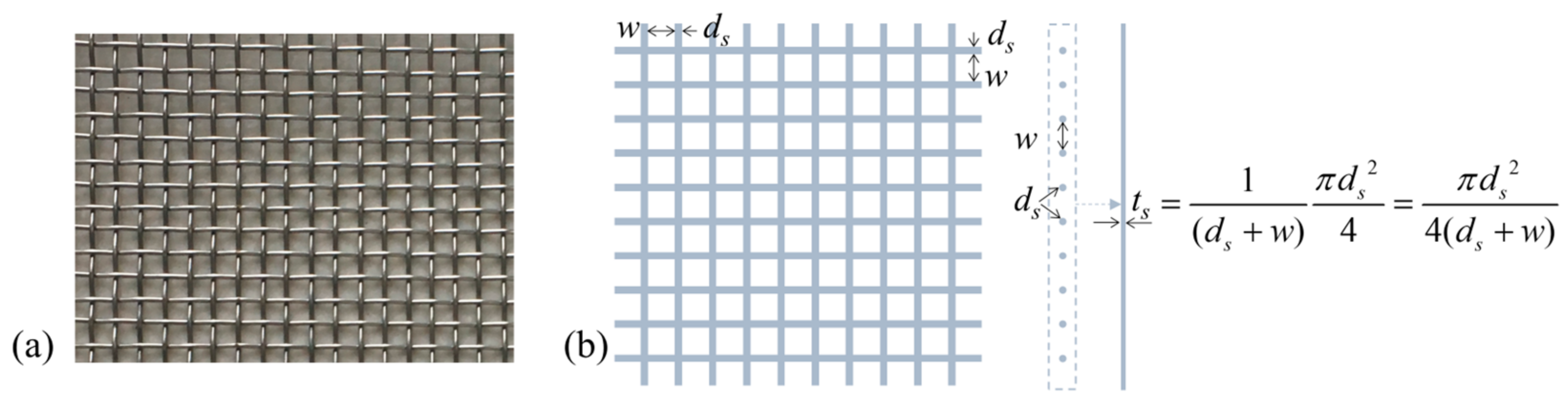
Figure 2 exhibits the configuration of real steel woven wire mesh reinforcement. It is made up of separate steel wires woven in orthogonal directions, without bonding at the intersections. These steel wires have the same diameter of d_s, and the apertures in the mesh reinforcement have the same dimension of $w\times w$. However, the mesh structure of the reinforcement makes it difficult to analyze its mechanical response. To address this, in the analytical model, the steel mesh reinforcement is simplified to a continuous solid layer with an equivalent thickness t_s. The value of t_s is determined by ensuring that the tensile stress in the continuous solid layer remains equivalent to that in the original discrete steel wires. Since these steel wires have no bonding at the intersections, the deformation of steel wires in one direction does not cause the deformation of steel wires in the perpendicular direction. The Poisson’s ratio of the equivalent solid layer should be zero, as well as the in-plane shear stress in the reinforcement. Similar properties can be found in fiber cloth reinforcement [31,33]. Moreover, with a zero Poisson’s ratio, the tensile force generated by rubber bulging in the reinforcement layer is independently borne by the reinforcing wires in each of the two directions. To maintain the same stress, the solid layer should have the same cross-sectional area (or volume) as the total area (or volume) of all the wires in one direction, as illustrated in Figure 2b. The equivalent thickness t_s is calculated to be $\pi d_s^2/[4(d_s+w)]$, which is only related to the characteristics of mesh reinforcement. Finite element analysis was then conducted in ANSYS 15.0 [34] on a specific bearing with different forms of reinforcement, but the same load and boundary conditions were used to validate this simplification method. More details about the validation of this method can refer to [35]. Figure 3 compares the stress in the two forms of reinforcement. It shows that the axial tensile stress in the mesh reinforcement has almost the same distribution and ranges with the normal stress in the solid reinforcement, demonstrating the validity of the simplification method.

Figure 4 illustrates the internal force and stress in an infinitesimal dx by dy area of the equivalent continuous solid reinforcement. $F_{xx},F_{yy}$ denote the normal forces of the reinforcement per unit length in the x and y directions, respectively. ${\tau }_{xz},{\tau }_{yz}$ are the shear stresses on the reinforcement surfaces, which are generated by the rubber layers bonded at the top and bottom of the reinforcement.

The equilibrium equations of reinforcement are as follows:

$$d{F}_{xx}dy+\left({\tau }_{xz}{|}_{z=-t/2}-{\tau }_{xz}{|}_{z=t/2}\right)dxdy=0$$

(13)

$$d{F}_{yy}dx+\left({\tau }_{yz}{|}_{z=-t/2}-{\tau }_{yz}{|}_{z=t/2}\right)dxdy=0$$

(14)

Substituting Equation (10) into Equations (13) and (14), and then applying Equation (11) to eliminate $u_0$ and $v_0$, the expressions of $F_{xx}$ and $F_{yy}$ in terms of p are obtained:

$$F_{xx,x}=t{p}_{,x}$$

(15)

$$F_{yy,y}=t{p}_{,y}$$

(16)

Considering the linearly elastic behavior of steel mesh reinforcement, the tensile strains $u_{1,x}$ and $v_{1,y}$ in the reinforcement along the x- and y-axis, respectively, are linearly related to the corresponding internal force $F_{xx}$ and $F_{yy}$:

$$\begin{array}{l}{u}_{1,x}=\frac{F_{xx}}{E_s{t}_s}\\ v_{1,y}=\frac{F_{yy}}{E_s{t}_s}\end{array}$$

(17)

where $E_s$ is the elastic modulus of the steel wire, and $t_s$ is the equivalent solid reinforcement thickness.

Integrating Equations (15) and (16) with respect to x and y, respectively, and then combining with Equation (17) lead to the following:

$$\begin{array}{l}{u}_{1,x}=\frac{t}{E_s{t}_s}p+f(y)\\ v_{1,y}=\frac{t}{E_s{t}_s}p+g(x)\end{array}$$

(18)

2.4. Approximate Boundary Conditions

No force is applied at the rubber layer’s side surface and the reinforcement’s end. Thus, the force boundary conditions of the rubber layer and the reinforcement should satisfy the following equations, respectively:

$$\begin{array}{cc}p(\pm a,y)=0& y\in [-b,b]\\ p(x,\pm b)=0& x\in [-a,a]\end{array}$$

(19)

$$\begin{array}{cc}{F}_{xx}(\pm a,y)=0& y\in [-b,b]\\ F_{yy}(x,\pm b)=0& x\in [-a,a]\end{array}$$

(20)

Considering Equation (17), the boundary conditions of internal force in Equation (20) are transformed into the boundary conditions of strain:

$$\begin{array}{cc}{u}_{1,x}(\pm a,y)=0& y\in [-b,b]\\ v_{1,y}(x,\pm b)=0& x\in [-a,a]\end{array}$$

(21)

2.5. Solution of Pressure

Substituting the boundary conditions of Equations (19) and (21) into Equation (18), the following are obtained:

$$\begin{gathered} f(y)=0 \\ g(x)=0 \end{gathered}$$

Then, the relationship between the strain and stress of the reinforcement in Equation (18) can be reduced to

$$\begin{array}{l}{u}_{1,x}=\frac{t}{E_s{t}_s}p\\ v_{1,y}=\frac{t}{E_s{t}_s}p\end{array}$$

(22)

Replacing Equations (12) and (22) into the strain compatibility equation of Equation (6), a differential equation in terms of p can be obtained:

$$p_{,xx}+p_{,yy}-\frac{24G}{E_s{t}_{s}t}p-\frac{12G}{K{t}^2}p=-\frac{12G{\epsilon }_c}{t^2}$$

(23)

Two constants are introduced here:

$$\alpha =\sqrt{\frac{12G}{E_s{t}_{s}t}}$$

(24)

$$\beta =\sqrt{\frac{12G}{K{t}^2}}$$

(25)

And Equation (23) is changed to the following form:

$$p_{,xx}+p_{,yy}-(2{\alpha }^2+{\beta }^2)p=-\frac{12G{\epsilon }_c}{t^2}$$

(26)

The two constants $\alpha$ and $\beta$ indicate the ductility of reinforcement and the compressibility of rubber, respectively. The reinforcement is more flexible at a higher value of $\alpha$. When $\alpha$ is reduced to zero, the reinforcement will behave like the rigid steel plate applied in common bearings. In the same way, the larger the $\beta$, the more pronounced the compression of the rubber volume. When $\beta$ becomes zero, the rubber turns incompressible.

To determine the solution of pressure p from Equation (26) with the boundary condition of Equation (19), p is assumed to be a function of a specific form [11,25,32,33] that satisfies the required boundary conditions. Then, the problem of solving the differential equation can be transformed into a problem of solving the unknown coefficients in the specific function. A double Fourier series form solution of p [32] is applied in this study. The internal pressure $p(x,y)$ and the constant term on the right-hand side in Equation (26) are expressed by the double Fourier series with unidentified coefficients $p_{nm}$ and $a_{nm}$, respectively:

$$p(x,y)={\displaystyle \sum _{n,m=1}^{\infty }{p}_{nm}}\cos (\frac{n\pi }{2a}x)\cos (\frac{m\pi }{2b}y)$$

(27)

$$-\frac{12G{\epsilon }_c}{t^2}={\displaystyle \sum _{n,m=1}^{\infty }{a}_{nm}\cos (\frac{n\pi }{2a}x)\cos (\frac{m\pi }{2b}y)}$$

(28)

where n and m are odd numbers to satisfy the boundary conditions in Equation (19). The coefficient $a_{nm}$ can be determined as follows:

$$a_{nm}=\frac{1}{ab}{\displaystyle {\int }_{-a}^a{\displaystyle {\int }_{-b}^b(-\frac{12G{\epsilon }_c}{t^2})\cos }}(\frac{n\pi }{2a}x)\cos (\frac{m\pi }{2b}y)dydx=-\frac{192G{\epsilon }_c}{mn{\pi }^2{t}^2}$$

(29)

Substituting Equations (27)–(29) into Equation (26), the coefficient $p_{nm}$ in Equation (27) is obtained:

$$p_{nm}=\frac{192G{\epsilon }_c}{mn{\pi }^2{t}^2}\frac{1}{{(\frac{n\pi }{2a})}^2+{(\frac{m\pi }{2b})}^2+2{\alpha }^2+{\beta }^2}$$

(30)

From Equations (27) and (30), the internal pressure p can be expressed by

$$p(x,y)={\displaystyle \sum _{k=1;n,m=2k-1}^{\infty }\frac{192G{\epsilon }_c}{mn{\pi }^2{t}^2}\frac{\cos (\frac{n\pi }{2a}x)\cos (\frac{m\pi }{2b}y)}{{(\frac{n\pi }{2a})}^2+{(\frac{m\pi }{2b})}^2+2{\alpha }^2+{\beta }^2}}$$

(31)

Integrating p over the upper surface of the rubber layer leads to the relationship between the vertical resultant force P and the rubber layer’s vertical compression strain ${\epsilon }_c$. Then, ${\epsilon }_c$ can be expressed as follows:

$${\epsilon }_c=\frac{{\pi }^4{t}^{2}P}{3072Gab}{\left[{\displaystyle \sum _{k=1;n,m=2k-1}^{\infty }\frac{1}{m^2{n}^2}\frac{1}{{(\frac{n\pi }{2a})}^2+{(\frac{m\pi }{2b})}^2+2{\alpha }^2+{\beta }^2}}\right]}^{-1}$$

(32)

2.6. Internal Forces in The Reinforcement

The internal force in the reinforcement $F_{xx}$ and $F_{yy}$ can be obtained by substituting the expression p in Equation (27) into Equation (15) and integrating with respect to x and y, respectively:

$$\begin{array}{l}{F}_{xx}=t{\displaystyle \sum _{n,m=1}^{\infty }{p}_{nm}}\cos (\frac{n\pi }{2a}x)\cos (\frac{m\pi }{2b}y)+C_1(y)\\ F_{yy}=t{\displaystyle \sum _{n,m=1}^{\infty }{p}_{nm}}\cos (\frac{n\pi }{2a}x)\cos (\frac{m\pi }{2b}y)+C_2(x)\end{array}$$

(33)

where $C_1(y)$ and $C_2(x)$ should be equal to zero in agreement with the boundary condition of $F_{xx}$ and $F_{yy}$ in Equation (20). $F_{xx}$ and $F_{yy}$ are reduced to the following:

$$F_{xx}=F_{yy}=t{\displaystyle \sum _{n,m=1}^{\infty }{p}_{nm}}\cos (\frac{n\pi }{2a}x)\cos (\frac{m\pi }{2b}y)$$

(34)

Substituting the expression of $p_{nm}$ into Equation (34), $F_{xx}$ and $F_{yy}$ follow

$$F_{xx}=F_{yy}={\displaystyle \sum _{k=1;n,m=2k-1}^{\infty }\frac{192G{\epsilon }_c}{mn{\pi }^{2}t}}\frac{\cos (\frac{n\pi }{2a}x)\cos (\frac{m\pi }{2b}y)}{{(\frac{n\pi }{2a})}^2+{(\frac{m\pi }{2b})}^2+2{\alpha }^2+{\beta }^2}$$

(35)

Finally, combining Equations (32) and (35), the internal forces of the reinforcement per unit length in the x and y directions, respectively, are provided in terms of vertical load P:

$$\begin{array}{cc}\hfill F_{xx}=& F_{yy}=\frac{{\pi }^{2}tP}{16ab}{\left[{\displaystyle \sum _{k=1;n,m=2k-1}^{\infty }\frac{1}{m^2{n}^2}\frac{1}{{(\frac{n\pi }{2a})}^2+{(\frac{m\pi }{2b})}^2+2{\alpha }^2+{\beta }^2}}\right]}^{\sum 1}\times \hfill \\ & \left[{\displaystyle \sum _{k=1;n,m=2k-1}^{\infty }\frac{1}{mn}}\frac{\cos (\frac{n\pi }{2a}x)\cos (\frac{m\pi }{2b}y)}{{(\frac{n\pi }{2a})}^2+{(\frac{m\pi }{2b})}^2+2{\alpha }^2+{\beta }^2}\right]\hfill \end{array}$$

(36)

The above equations demonstrate that the internal force of steel mesh reinforcement is positively correlated with the vertical load P and the individual rubber thickness t. Still, it is also negatively correlated with the flexibility of reinforcement and the compressibility of rubber.

Figure 5 plots the distribution of $F_{xx}$ and $F_{yy}$ over the cross-section of a USRB under a vertical compression of 70 MPa. The configurations and material properties of the investigated USRB are listed in

Table 1. Configurations and material properties of the USRB.

a	b	t	${\mathit{d}}_{\mathit{s}}$	w	G	K	${\mathit{E}}_{\mathit{s}}$
mm	mm	mm	mm	mm	MPa	MPa	MPa
200	200	2.0	0.8	1.8	1.0	2000	$2\times {10}^5$

, where a is half bearing width, b is half bearing length, t is the rubber layer thickness, ds is steel wire diameter, w is the aperture dimension of steel wire mesh reinforcement, G is the rubber shear modulus, K is the rubber bulk modulus, and E_s is the reinforcement elastic modulus.

It can be seen from Figure 5 that $F_{xx}$ and $F_{yy}$ are identical. It implies that the internal forces of reinforcement at a given point are the same in the x and y directions. In addition, $F_{xx}$ and $F_{yy}$ reach their maximum $F_{xx\max }$ and $F_{yy\max }$ at the center of the cross-section, where x = 0 and y = 0. As a result, it is anticipated that the failure of USRBs is initiated by the tensile failure of the reinforcement at the center.

3. Analytical Solution of Ultimate Compression Capacity of Rectangular USRBs

According to a previous test study, when USRBs’ vertical pressure load reaches $p_u$, the reinforcement’s maximum tensile stress ${\sigma }_{\max }$ reaches the steel wire’s ultimate tensile strength $f_u$. As such, further investigation is conducted to explore the analytical solution for the ultimate compression capacity $p_u$, building upon the above analysis of the internal force F in the mesh reinforcement.

The resultant force P of the upper surface corresponding to the ultimate compressive loading $p_u$ is

$$P=4ab{p}_u$$

(37)

Substituting the above equation into Equation (36) under the condition of x = 0 and y = 0, the maximum internal force of reinforcement per unit length $F_{\max }$ at load $p_u$ is obtained:

$$\begin{array}{cc}\hfill F_{xx\max }=F_{yy\max }=F_{\max }=& \frac{{\pi }^{2}t{p}_u}{4}{\left[{\displaystyle \sum _{k=1;n,m=2k-1}^{\infty }\frac{1}{m^2{n}^2}\frac{1}{{(\frac{n\pi }{2a})}^2+{(\frac{m\pi }{2b})}^2+2{\alpha }^2+{\beta }^2}}\right]}^{-1}\times \hfill \\ & \left[{\displaystyle \sum _{k=1;n,m=2k-1}^{\infty }\frac{1}{mn}}\frac{1}{{(\frac{n\pi }{2a})}^2+{(\frac{m\pi }{2b})}^2+2{\alpha }^2+{\beta }^2}\right]\hfill \end{array}$$

(38)

As previously stated, the tensile stress in the continuous solid layer remains equivalent to that in the original discrete steel wires. Then, the relationship between the maximum tensile stress of steel wires ${\sigma }_{\max }$ and the maximum internal force of reinforcement $F_{\max }$ is determined as

$${\sigma }_{\max }=\frac{F_{\max }}{t_s}=\frac{4F_{\max }(d_s+w)}{\pi d_s^2}$$

(39)

Substituting the expression of $F_{\max }$ at load $p_u$ into the above equation, the expression of the maximum tensile stress of reinforcement ${\sigma }_{\max }$ at ultimate load $p_u$ is obtained:

$$\begin{array}{rr}{\sigma }_{\max }=\frac{\pi t{p}_u(d_s+w)}{d_s^2}& {\left[{\displaystyle \sum _{k=1;n,m=2k-1}^{\infty }\frac{1}{m^2{n}^2}\frac{1}{{(\frac{n\pi }{2a})}^2+{(\frac{m\pi }{2b})}^2+2{\alpha }^2+{\beta }^2}}\right]}^{-1}\hfill \\ & \times \left[{\displaystyle \sum _{k=1;n,m=2k-1}^{\infty }\frac{1}{mn}}\frac{1}{{(\frac{n\pi }{2a})}^2+{(\frac{m\pi }{2b})}^2+2{\alpha }^2+{\beta }^2}\right]\hfill \end{array}$$

(40)

A commonly used characteristic parameter A₀ that measures the open area of the steel mesh reinforcement is defined in Equation (41) [36]. It is the ratio of the area of total apertures to the area of steel mesh reinforcement. A₀ is a critical parameter commonly listed in the specification table of steel wire mesh.

$$A_0=100{(\frac{w}{w+d_s})}^2$$

(41)

As previously mentioned, the maximum tensile stress of reinforcement ${\sigma }_{\max }$ is equal to the tensile strength $f_u$ of steel wires at the vertical load of $p_u$. From Equations (40) and (41), the ultimate compression capacity $p_u$ of rectangular USRBs is expressed by

$$\begin{array}{cc}\hfill p_u=\frac{f_u{d}_s}{\pi t}(1-\sqrt{\frac{A_0}{100}})& \left[{\displaystyle \sum _{k=1;n,m=2k-1}^{\infty }\frac{1}{m^2{n}^2}\frac{1}{{(\frac{n\pi }{2a})}^2+{(\frac{m\pi }{2b})}^2+2{\alpha }^2+{\beta }^2}}\right]\hfill \\ & \times {\left[{\displaystyle \sum _{k=1;n,m=2k-1}^{\infty }\frac{1}{mn}}\frac{1}{{(\frac{n\pi }{2a})}^2+{(\frac{m\pi }{2b})}^2+2{\alpha }^2+{\beta }^2}\right]}^{-1}\hfill \end{array}$$

(42)

The analytical solution of $p_u$ implies that $p_u$ is affected by the configurations of USRBs and the material properties of rubber and steel mesh reinforcement, including bearing width a, bearing length b, rubber layer thickness t, reinforcement wire diameter d_s, reinforcement open area ratio A₀, reinforcement elastic modulus E_s, reinforcement tensile strength f_u, rubber shear modulus G, and rubber bulk modulus K. To further study the influence of these factors/parameters, a series of USRB samples, with different configurations and material properties, are compared on their theoretical ultimate loading capacity $p_u$. The benchmark values for each impact factor are listed in Table 1, and the benchmark value for A₀ is 48. Figure 6a–d compare the variations in USRBs’ normalized ultimate compression capacity $p_u/f_u$ with different factors, whose values range from 0.5 to 2.0 times the benchmark values.

The results in Figure 6 show that the ultimate compression capacity $p_u$ of USRBs is positively correlated with bearing width a, the bearing length-to-width ratio b/a, and reinforcement wire diameter d_s. In contrast, it is negatively correlated with rubber layer thickness t, the reinforcement open area ratio A₀, the normalized reinforcement elastic modulus $E_s/G$, and the normalized rubber bulk modulus $K/G$. The results in Figure 6 are consistent with previous test observations [9], where USRB specimens with larger plan areas (i.e., a), larger steel wire diameters (i.e., d_s), and smaller rubber layer thickness (i.e., t_s) exhibited higher compression capacities $p_u$. The effects of E_s and K demonstrate that the reinforcement flexibility and rubber compressibility would enhance the bearings’ ultimate compression capacity. In addition, the influence of t, d_s, and A₀ are prominent among all the factors, whereas the effect of $E_s/G$ and $K/G$ are negligible. Furthermore, the comparisons between each two factors indicate that increasing bearing width a is more effective in enlarging p_u than increasing the length-to-width ratio b/a (Figure 6a). Analogously, to enlarge p_u, decreasing rubber layer thickness t is more efficient than increasing the reinforcement wire diameter d_s (Figure 6b), and increasing d_s is more efficient than reducing the reinforcement open area ratio A₀ (Figure 6c).

4. Ultimate Compression Test Results of USRB

A total of 19 USRB specimens [9], as listed in

Table 2. Configurations of tested USRB specimens.

No.	a (mm)	b (mm)	ds (mm)	t (mm)	ns	A0	pu_test (MPa)	pu_analytical (MPa)
1	69	94	0.8	3.3	5	48	50	70
2	95	120	0.8	2.5	21	48	70	109
3	95	120	0.8	2.5	21	48	68	109
4	95	120	0.8	2.5	21	48	68	109
5	95	120	0.8	3	17	48	59	86
6	95	120	0.8	3	17	48	64	86
7	95	120	0.8	3	21	48	71	86
8	95	120	0.8	3	21	48	66	86
9	95	120	0.8	3	21	48	67	86
10	95	120	0.8	3.5	15	48	50	70
11	95	120	0.8	3.5	15	48	51	70
12	95	120	0.8	3.5	21	48	30	70
13	95	120	0.8	3.5	21	48	51	70
14	95	120	0.8	4	13	48	42	59
15	95	120	0.8	4	13	48	41	59
16	117	142	0.8	3.6	13	48	50	71
17	120	145	0.6	5.6	9	56	17	26
18	140	190	0.8	2.8	7	48	76	101
19	140	190	0.8	3.8	5	48	60	69

Notes: a: half bearing width; b: half bearing length; d_s: steel wire diameter; t: individual rubber layer thickness; n_s: number of reinforcement layers; A₀: reinforcement open area ratio; p_u_test: ultimate compression capacity test results; p_u_analytical: ultimate compression capacity analytical solutions.

, were tested to validate the analytical solutions for ultimate compression capacities p_u. During the tests, the specimens exhibited continuous cracking sounds, and cross-sectional inspection after tests confirmed the fracture of steel wires in the reinforcement. This demonstrates that the failure of USRB under compression originates from the fracture failure of steel wires. Therefore, it is reasonable for the analytical USRB model to consider the compressive stress at the fracture of steel mesh reinforcements as the ultimate strength p_u. Material properties of rubber and the geometric characteristics of steel mesh reinforcement were provided by the manufacturers. The shear modulus (G) and bulk modulus (K) of rubber were 1.0 MPa and 2000 MPa, respectively. Axial tensile tests were carried out on the steel wires to obtain their elastic modulus (E_s) and tensile strength (f_u). The measured stress–strain curves for three steel wire specimens are displayed in Figure 7. According to Figure 6d, E_s demonstrates negligible influence on the compression capacity. The elastic modulus (E_s) was then decided by the secant modulus E1, E2, and E3 to simulate the stress and strain responses at tensile failure. The average E_s and f_u for the steel wire are 7250 MPa and 1450 MPa, respectively. The p_u analytical solutions were derived using Equation (42) and are listed in Table 2.

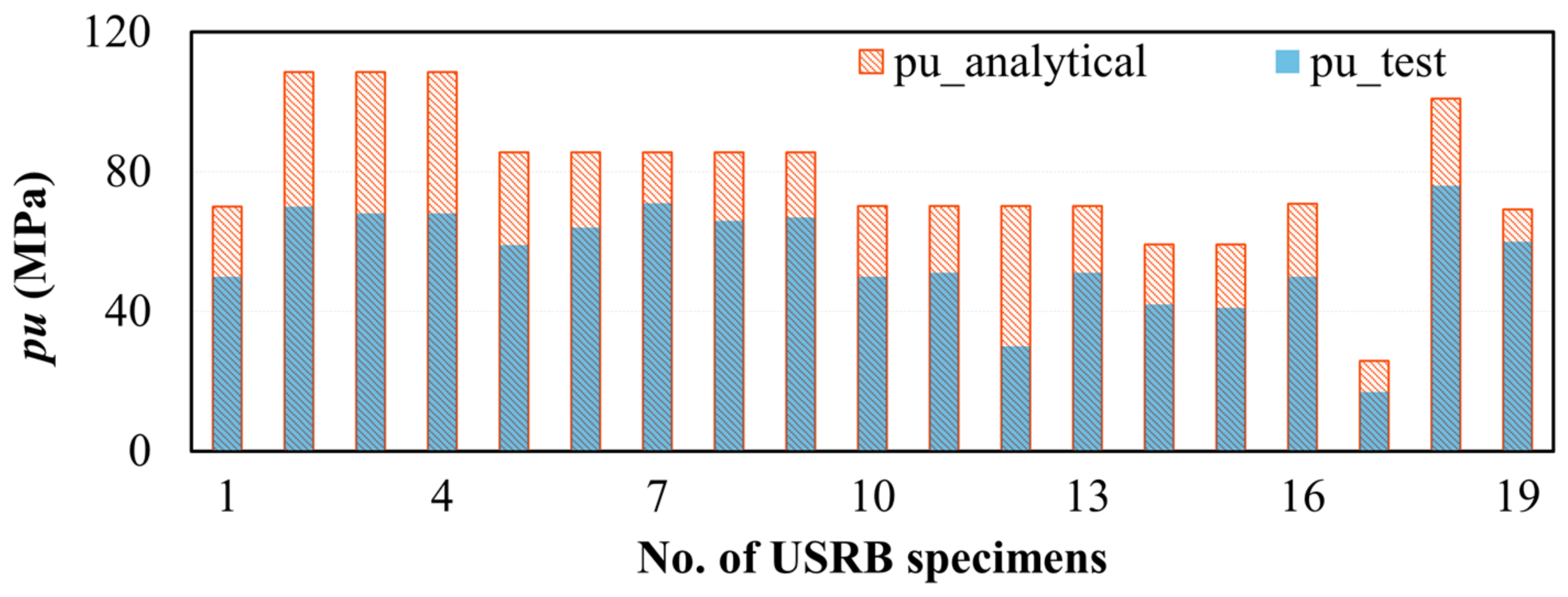
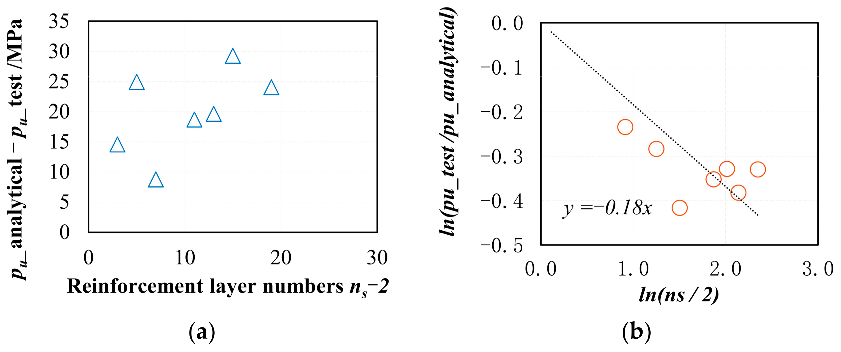
Figure 8 compares the analytical solutions of ultimate compression capacities (p_u) with corresponding test results. The analytical solution significantly overestimates the test results, with a mean absolute error (MAE) of 23.1 MPa and a root-mean-square error (RMSE) of 25.0 MPa. This significant discrepancy is attributed to the simplification of the USRB analytical model, which assumes equal mechanical performance for all rubber layers. However, Tsai [37] analyzed the fiber-reinforced bearings with multiple rubber layers, and found that the mechanical performance of each rubber layer is not the same. Moreover, test results show that USRB specimens with more reinforcement layers n_s (or rubber layers) tend to have lower p_u results. For example, specimen No. 12 is identical to specimen No. 11 except having more reinforcement layers (i.e., 21 layers) than No. 11 (i.e., 15 layers). The p_u of No. 12 is smaller (30 MPa) compared to that of No. 11 (50 MPa). This might be due to the fact that bearings with more rubber or reinforcement layers tend to suffer buckling failure or eccentric compression. This finding suggests that the number of reinforcement layers n_s or rubber layers has an impact on the ultimate compression capacity, whereas the simplified analytical model with only one rubber layer (n_s = 2) cannot consider this impact. Figure 9a further demonstrates the correlation between estimation errors (i.e., difference between p_u analytical solution and test result) and the difference in reinforcement layer number between test specimens and the analytical model n_s − 2, with larger n_s causing higher discrepancy. Therefore, calibration of the p_u analytical solution based on the test results is necessary to account for the effect of n_s on the ultimate compression capacity. Notably, p_u analytical results with the same n_s were averaged on their errors in Figure 9.

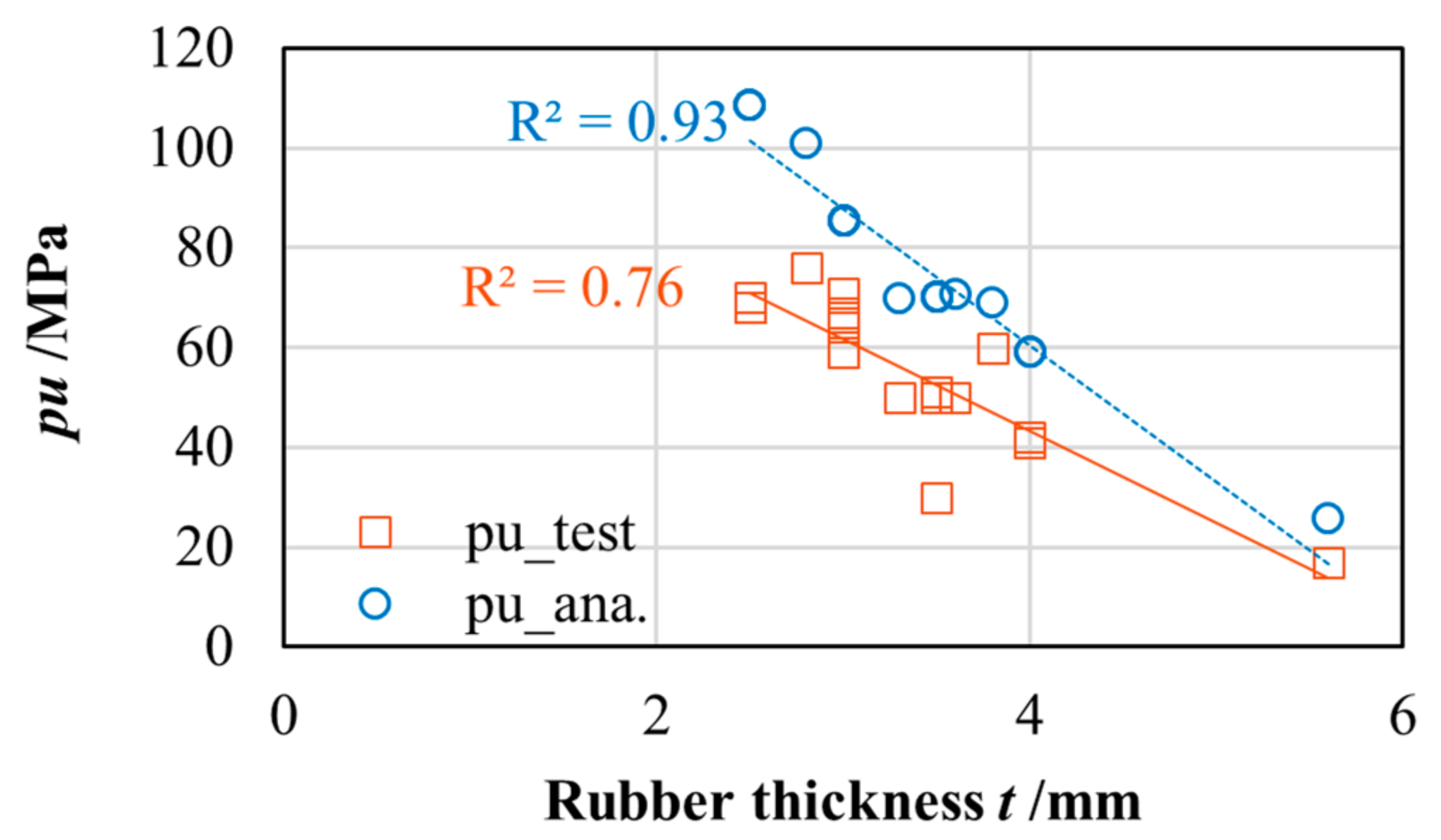
Despite the significant discrepancy of the p_u value, p_u analytical solutions can capture the variation in p_u with rubber thickness t. Figure 10 illustrates the correlation between rubber layer thickness t and p_u from test results. It shows that p_u decreases significantly as t increases. This aligns with previous finite element model analysis results [38]. Figure 10 also compares the variation in p_u with t between the analytical solution and test results. The trend of analytical solutions is consistent with that of test results despite the discrepancy in values.

As stated above, the different values of n_s between the analytical model and real USRB specimens leads to the error of p_u analytical solutions. Calibration was conducted to include the effect of n_s in the analytical solution. When the tested USRB specimen has the same reinforcement layer number as the simplified analytical model (i.e., n_s = 2), its ultimate compression capacity should be equal to the analytical solution. An assumption was then made that the p_u_test should be equal to p_u analytical solutions when n_s = 2. Based on engineering judgements, the relation between p_u_test/p_u_analytical should follow

$$\ln \left(\frac{p_u\_test}{p_u\_analytical}\right)=m_0\ln \left(\frac{n_s}{2}\right)$$

(43)

Figure 9b presents the relationship between n_s and the average ratio of p_u test results to p_u analytical solutions (p_u_test/p_u_analytical) at each n_s level. The coefficient m₀ in Equation (43) is determined to be −0.18 from the linear regression results. It leads to

$$p_u\_test={\left(\frac{n_s}{2}\right)}^{-0.18}{p}_u\_analytical$$

(44)

The calibration term in Equation (44) was introduced in the p_u analytical solution in Equation (42) to improve accuracy. The calibrated analytical solution of ultimate compression capacity p_u yields to the following:

$$\begin{array}{cc}\hfill p_u={\left(\frac{n_s}{2}\right)}^{-0.18}\frac{f_u{d}_s}{\pi t}(1-& \sqrt{\frac{A_0}{100}})\left[{\displaystyle \sum _{k=1;n,m=2k-1}^{\infty }\frac{1}{m^2{n}^2}\frac{1}{{(\frac{n\pi }{2a})}^2+{(\frac{m\pi }{2b})}^2+2{\alpha }^2+{\beta }^2}}\right]\times \hfill \\ & {\left[{\displaystyle \sum _{k=1;n,m=2k-1}^{\infty }\frac{1}{mn}}\frac{1}{{(\frac{n\pi }{2a})}^2+{(\frac{m\pi }{2b})}^2+2{\alpha }^2+{\beta }^2}\right]}^{-1}\hfill \end{array}$$

(45)

The calibration term ${\left(n_s/2\right)}^{-0.18}$ is consistent with the test results that n_s is negatively correlated with p_u. Figure 11 compares the p_u_calibrated values with the p_u_test results for all specimens, demonstrating a strong fit for the regression set. The mean absolute error and root-mean-square error of p_u_calibrated compared to p_u_test are 4.9 MPa and 6.8 MPa, respectively, significantly reducing the estimation error compared to the analytical results (i.e., MAE = 23.1 MPa, RMSE = 25.0 MPa) in Figure 8.

It should be noted that the p_u calibrated solution presented here is intended to estimate the exact ultimate compression capacity of USRBs, rather than its lower bound. Thus, the reliability of the p_u calibrated solution is not the main concern. The p_u calibrated solution proposed here can be applied during the preliminary design stage for the optimization design of USRBs by providing a close estimation of p_u. The actual ultimate compression capacity of an optimized USRB prototype should always be examined via tests before USRBs are applied in structures.

5. An Efficient Solution for the Ultimate Compression Capacity of Rectangular USRB

To facilitate engineering applications, an efficient solution of p_u was proposed by considering all important parameters:

$$p_u=n_0{f}_u{\left(\frac{n_s}{2}\right)}^{-0.18}{\left(\frac{a}{t}\right)}^{n_1}{\left(\frac{b}{a}\right)}^{n_2}{\left(\frac{t_f}{t}\right)}^{n_3}\left(1-\sqrt{\frac{A_0}{100}}\right){\left(\frac{G}{E_s}\right)}^{n_4}{\left(\frac{G}{K}\right)}^{n_5}$$

(46)

where n_i (i = 0~5) are coefficients to be determined by the multiple linear regression with a large set of calibrated analytical p_u results.

The efficient solution accounts for four geometric parameters (a, b/a, t, and d_s) and four material parameters (A₀, G, E_s, and K). To determine the coefficients, various USRB samples with different configurations and material properties were analyzed for their ultimate compression capacities. The number of reinforcement layers n_s in all samples was set to 2 to eliminate its influence.

Table 3. Various configurations and material properties of USRBs.

a (mm)	b/a	t (mm)	ds (mm)	A0 (%)	G (MPa)	Es (MPa)	K (MPa)
50	1.00	1	0.02	25	0.4	2.00 × 103	1000
125	1.25	2	0.50	40	0.8	5.00 × 104	2000
200	1.50	3	1.00	55	1.2	1.00 × 105	4000
275	1.75	4	1.40	70	1.6	1.50 × 105	6000
350	2.00	5	2.00	86	2.0	2.00 × 105	8000

summarizes the geometric configurations and material properties of these samples, covering a range of values for parameters such as bearing width a, length-to-width ratio b/a, rubber layer thickness t, reinforcement wire diameter d_s, reinforcement open area ratio A₀, rubber shear modulus G, reinforcement elastic modulus E_s, and rubber bulk modulus K. These parameters were varied at different levels to cover all possible cases and broaden the application of p_u efficient solutions. The samples consisted of 5⁸ combinations of these parameters. Limitations were applied to ensure the reasonableness of the bearing configurations. These included not exceeding the maximum cross-section area for small-to-medium-span highway bridges (700 mm × 700 mm for unbonded laminated rubber bearings as per the Ministry of Transport of the People’s Republic of China, 2004), ensuring that the rubber layer thickness is greater than the reinforcement thickness, and matching the reinforcement open area ratio to the reinforcement thickness according to the steel woven wire mesh reinforcement specification table [36].

A total of 182,875 USRB samples with reasonable configurations were studied. The p_u calibrated solution was applied to calculate the calibrated analytical p_u for these samples using Equation (45), where f_u takes the mean value of 1450 MPa. Multiple linear regression was conducted on the calibrated p_u results and corresponding factors to obtain the constant coefficients in Equation (46). The least square method minimized the sum of squared errors to determine the coefficients: n₀ = 0.688, n₁ = 0.192, n₂ = 0.100, n₃ = 0.950, n₄ = 0.067, and n₅ = 0.038. This leads to the efficient solution of p_u:

$$p_u=0.688f_u{\left(\frac{n_s}{2}\right)}^{-0.18}{\left(\frac{a}{t}\right)}^{0.192}{\left(\frac{b}{a}\right)}^{0.100}{\left(\frac{d_s}{t}\right)}^{0.950}\left(1-\sqrt{\frac{A_0}{100}}\right){\left(\frac{G}{E_s}\right)}^{0.067}{\left(\frac{G}{K}\right)}^{0.038}$$

(47)

Figure 12 compares the estimated p_u (empirical p_u) from Equation (47) with the calibrated analytical p_u results. The mean absolute error (MAE) value and mean squared error (MSE) value of the multiple linear regression are 3.9 and 45.2, respectively, with a coefficient of determination, R², close to 1.0. This implies that the efficient solution of p_u in Equation (47) reasonably predicts the calibrated analytical p_u from Equation (45).

Considering the wide range of USRBs investigated in terms of configurations and material properties, the generalized efficient solution of p_u in Equation (47) can be used for all USRBs. Figure 13 compares the empirical p_u results, calibrated analytical p_u results, and test p_u results for the specimens in Table 2. The empirical p_u results coincide with the calibrated analytical solutions and accurately predict the majority of the test p_u results. The mean relative error for the empirical p_u results is 25%. Therefore, the efficient solution of p_u in Equation (47) can serve as a simple method to estimate the ultimate compression capacity of USRBs in practical engineering applications.

Moreover, the regressed coefficients in Equation (47) also indicate the relative importance of each factor for the compression capacity, with a larger value representing higher correlation. The regression results align with the parametric study in Figure 6, where the correlation between each parameter with compression capacity, arranged in descending order, is as follows: t, d_s, A₀, a, n_s, a/b, G, E_s, and K.

6. Preliminary Design of USRB

In this section, we illustrate the optimization design process of USRBs during the preliminary design stage, using the proposed analytical solutions. The cross-section size (a and b) is determined based on the weight of superstructures. The bearing height H is set according to the seismic deformation demand. Material properties, including the rubber shear modulus G, rubber bulk modulus K, steel mesh elastic modulus E_s, tensile strength f_u, and steel mesh open area ratio A₀, are typically provided by the manufacturers. Geometric parameters like individual rubber thickness t, reinforcement wire diameter d_s, and the number of reinforcement layers n_s, can be decided based on the ultimate loading carrying capacity requirement of USRBs.

For example, consider the design of USRBs in a single-span simply supported girder bridge. The bridge’s superstructure is supported by twenty USRBs, with ten at each end. The total vertical design load is 2100 tons, considering both dead and live loads. The maximum relative seismic displacement between the girder and substructure is 120 mm.

Using the given information, the vertical load per USRB is 1050 kN, and the lateral deformation capacity of all USRBs should exceed 120 mm. Based on design criteria, the vertical design pressure is set at 10 MPa [39], and the lateral deformation capacity is 1.65 times the bearing height H [8,9]. Consequently, the cross-section of the bearing $2a\times 2b$ and height H are determined to be 300 mm × 350 mm and 75 mm, respectively.

The ultimate loading capacity requirement for USRBs is 70 MPa, matching the standard for unbonded laminated rubber bearings [39]. By substituting known parameters into Equation (45) and assuming material properties from Section 4, the rubber layer thickness t, reinforcement wire diameter d_s, and the number of reinforcement layers n_s must satisfy the following equation:

$$\begin{array}{l}{p}_u=0.688\times 1450\times {\left(\frac{n_s}{2}\right)}^{-0.18}{\left(\frac{150}{t}\right)}^{0.192}{\left(\frac{175}{150}\right)}^{0.100}{\left(\frac{d_s}{t}\right)}^{0.950}\left(1-\sqrt{\frac{48}{100}}\right){\left(\frac{1}{7250}\right)}^{0.067}{\left(\frac{1}{2000}\right)}^{0.038}\\ \ge 70MPa\end{array}$$

(48)

which leads to

$$t\le 4.41\times d_s^{0.832}{n}_s^{-0.158}$$

(49)

On the other hand, the rubber layer thickness t can be determined by the following:

$$t=\frac{H-2c_0-2n_s{t}_s}{n_s-1}$$

(50)

where c₀ is the top/bottom rubber cover thickness, and t_s is the equivalent thickness of mesh reinforcement illustrated in Figure 2. In this case, t_s is calculated to be 0.241 d_s. Substituting Equation (50) into Equation (49), the relation between d_s and n_s is obtained:

$$0.483d_s{n}_s^{1.158}+4.41d_s^{0.832}{n}_s-(H-2c_0)n_s^{0.158}-4.41d_s^{0.832}\ge 0$$

(51)

To ensure a standard ultimate compression capacity of over 70 MPa, the minimum number of reinforcement layers n_s can be estimated using Equation (51), considering a predetermined reinforcement wire diameter d_s obtained from the steel wire mesh specification table. Typically, n_s is minimized to reduce the cost and weight of USRBs. Subsequently, the rubber layer thickness t can be calculated using Equation (50).

In this example, d_s is initially set at 1 mm. Given a bearing height H of 75 mm and a top/bottom rubber cover thickness c₀ of 2.5 mm, Equation (51) estimates a minimum of 13 reinforcement layers n_s. The corresponding d_s is 2 mm. By using Equation (50), t is calculated to be 4.8 mm. The estimated ultimate compression capacity with this configuration is 77.6 MPa, meeting the required minimum of 70 MPa.

Following the above design process, the geometric configuration of USRB is determined, which satisfies both the lateral deformation and the vertical loading requirements. However, this design process does not address the seismic effectiveness of the bearing, which needs further structural dynamic analysis.

7. Conclusions

This study theoretically analyzed the ultimate compression capacity of the unbonded steel-mesh-reinforced rubber bearings (USRBs). Based on previous studies on fiber-reinforced rubber bearings, a simplified USRB analytical model, consisting of a single rubber layer and two flexible steel mesh reinforcements, was investigated for its performance under vertical compression, assuming that all materials are linearly elastic and the rubber is compressible. The closed-form solution of the internal force of the steel mesh reinforcement was derived via the stress method of elasticity theory. The analytical solution of USRBs’ ultimate compression capacity p_u was deduced from the fact that USRBs will suffer compression failure when the steel wire in the reinforcements breaks at its tensile strength. A parametric study on the influence of individual rubber thickness, bearing width, length-to-width ratio, reinforcement wire diameter, reinforcement open area ratio, reinforcement elastic modulus, and rubber bulk modulus was carried out to provide suggestions on improving USRBs’ ultimate compression capacity. Furthermore, the analytical solution of p_u was calibrated by the test results of 19 USRB specimens to consider the influence of the number of reinforcement layers n_s. Based on the calibrated p_u solution, an efficient solution of simplified form for the ultimate compression capacity was promoted, employing multiple linear regression with the calibrated analytical p_u results of 182,875 USRB samples. Finally, the design process of USRBs with specific ultimate compression capacity was illustrated based on the proposed efficient p_u solution. From the above investigations, the following main conclusions can be drawn:

• The failure of USRBs is initiated by the tensile failure of reinforcement at the center, since $F_{xx}$ and $F_{yy}$ reach their maximum $F_{xx\max }$ and $F_{yy\max }$ at the center of the cross-section.
• The ultimate compression capacity $p_u$ of USRB is positively correlated with the bearing width a, bearing length-to-width ratio b/a, and reinforcement wire diameter d_s. In contrast, it is negatively correlated with rubber layer thickness t, reinforcement open area ratio A₀, normalized reinforcement elastic modulus $E_s/G$, and normalized rubber bulk modulus $K/G$. Decreasing the rubber layer thickness t, increasing the reinforcement wire diameter d_s, and reducing reinforcement open area ratio A₀ can significantly enhance p_u, while increasing the reinforcement flexibility and rubber compressibility have a negligible effect. In addition, increasing bearing width a is more effective in enlarging p_u than increasing the length-to-width ratio b/a, and increasing d_s is more efficient than reducing the reinforcement open area ratio A₀.
• The influence of rubber layer thickness on the ultimate compression capacity in test results coincides with that of analytical results. However, a significant difference was observed between the p_u analytical solutions and p_u test results due to the simplification of USRB’s analytical model, which cannot account for the effect of the number of reinforcement layers on p_u, as observed in the tests.
• The p_u calibrated solution incorporates the influence of the number of reinforcement layers n_s and improves the estimation accuracy of the p_u test results. The calibrated solution was found to reduce the mean absolute error of the p_u analytical solution from 23.1 MPa to 4.9 MPa.
• The regressed efficient solution of p_u has a simpler form but the same accuracy as the calibrated solution in predicting the ultimate compression capacity, which could facilitate the preliminary design of USRBs in practical engineering.

References

- Kelly, J.M.; Konstantinidis, D. Effect of Friction on Unbonded Elastomeric Bearings. J. Eng. Mech. 2009, 135, 953–960. [Google Scholar] [CrossRef]
- Wu, G.; Wang, K.; Lu, G.; Zhang, P. An Experimental Investigation of Unbonded Laminated Elastomeric Bearings and the Seismic Evaluations of Highway Bridges with Tested Bearing Components. Shock Vib. 2018, 2018, 8439321. [Google Scholar] [CrossRef]
- Zhou, L.; Shahria Alam, M.; Song, A.; Ye, A. Probability-Based Residual Displacement Estimation of Unbonded Laminated Rubber Bearing Supported Highway Bridges Retrofitted with Transverse Steel Damper. Eng. Struct. 2022, 272, 115053. [Google Scholar] [CrossRef]
- Zhong, H.; Yuan, W.; Dang, X.; Deng, X. Seismic Performance of Composite Rubber Bearings for Highway Bridges: Bearing Test and Numerical Parametric Study. Eng. Struct. 2022, 253, 113680. [Google Scholar] [CrossRef]
- Mazza, F.; Labernarda, R. Internal Pounding between Structural Parts of Seismically Isolated Buildings. J. Earthq. Eng. 2022, 26, 5175–5203. [Google Scholar] [CrossRef]
- Han, Q.; Du, X.; Liu, J.; Li, Z.; Li, L.; Zhao, J. Seismic Damage of Highway Bridges during the 2008 Wenchuan Earthquake. Earthq. Eng. Eng. Vib. 2009, 8, 263–273. [Google Scholar] [CrossRef]
- Xiang, N.; Alam, M.S.; Li, J. Shake Table Studies of a Highway Bridge Model by Allowing the Sliding of Laminated-Rubber Bearings with and without Restraining Devices. Eng. Struct. 2018, 171, 583–601. [Google Scholar] [CrossRef]
- Li, H.; Tian, S.; Dang, X.; Yuan, W.; Wei, K. Performance of Steel Mesh Reinforced Elastomeric Isolation Bearing: Experimental Study. Constr. Build. Mater. 2016, 121, 60–68. [Google Scholar] [CrossRef]
- Li, H. Theoretical and Experimental Study on the High-Performance Seismic Isolation Technology for Short-to-Medium Span Bridges; Tongji University: Shanghai, China, 2022. [Google Scholar]
- Li, H.; Xie, Y.; Gu, Y.; Tian, S.; Yuan, W.; DesRoches, R. Shake Table Tests of Highway Bridges Installed with Unbonded Steel Mesh Reinforced Rubber Bearings. Eng. Struct. 2020, 206, 110124. [Google Scholar] [CrossRef]
- Kelly, J.M. Analysis of Fiber-Reinforced Elastomeric Isolators. J. Seismol. Earthq. Eng. 1999, 2, 19–34. [Google Scholar]
- Kim, D.J.; El-Tawil, S.; Naaman, A.E. Rate-Dependent Tensile Behavior of High Performance Fiber Reinforced Cementitious Composites. Mater. Struct. Constr. 2009, 42, 399–414. [Google Scholar] [CrossRef]
- Bakhshi, A.; Jafari, M.H.; Valadoust Tabrizi, V. Study on Dynamic and Mechanical Characteristics of Carbon Fiber- and Polyamide Fiber-Reinforced Seismic Isolators. Mater. Struct. Constr. 2014, 47, 447–457. [Google Scholar] [CrossRef]
- Losanno, D.; Calabrese, A.; Madera-Sierra, I.E.; Spizzuoco, M.; Marulanda, J.; Thomson, P.; Serino, G. Recycled versus Natural-Rubber Fiber-Reinforced Bearings for Base Isolation: Review of the Experimental Findings. J. Earthq. Eng. 2022, 26, 1921–1940. [Google Scholar] [CrossRef]
- Flora, A.; Calabrese, A.; Cardone, D. Identification and Calibration of Advanced Hysteresis Models for Recycled Rubber–Fiber-Reinforced Bearings. Buildings 2023, 13, 65. [Google Scholar] [CrossRef]
- Banerjee, S.; Matsagar, V. Hybrid Vibration Control of Hospital Buildings against Earthquake Excitations Using Unbonded Fiber-Reinforced Elastomeric Isolator and Tuned Mass Damper. Buildings 2023, 13, 1724. [Google Scholar] [CrossRef]
- Shrestha, B. Vertical Ground Motions and Its Effect on Engineering Structures: A State-of-the-Art Review. In Proceedings of the International Seminar on Hazard Management for Sustainable Development, Kathmandu, Nepal, 28 November 2009; pp. 190–202. [Google Scholar]
- Kunnath, S.K.; Erduran, E.; Chai, Y.H.; Yashinsky, M. Effect of Near-Fault Vertical Ground Motions on Seismic Response of Highway Overcrossings. J. Bridge Eng. 2008, 13, 282–290. [Google Scholar] [CrossRef]
- Ministry of Transport of the People’s Republic of China. Specifications for Seismic Design of Highway Bridges; Ministry of Transport of the People’s Republic of China: Beijing, China, 2020.
- Hedayati Dezfuli, F.; Alam, M.S. Performance of Carbon Fiber-Reinforced Elastomeric Isolators Manufactured in a Simplified Process: Experimental Investigations. Struct. Control Health Monit. 2014, 21, 1347–1359. [Google Scholar] [CrossRef]
- Losanno, D.; Madera Sierra, I.E.; Spizzuoco, M.; Marulanda, J.; Thomson, P. Experimental Assessment and Analytical Modeling of Novel Fiber-Reinforced Isolators in Unbounded Configuration. Compos. Struct. 2019, 212, 66–82. [Google Scholar] [CrossRef]
- Riyadh, M.M.; Osman, S.S.; Alam, M.S. Experimental Investigation of Novel Carbon-Fiber Reinforced Elastomeric Isolators with Polyurethane Cores under Vertical and Lateral Loading. Eng. Struct. 2023, 275, 115186. [Google Scholar] [CrossRef]
- Vemuru, V.S.M.; Nagarajaiah, S.; Mosqueda, G. Coupled Horizontal–Vertical Stability of Bearings under Dynamic Loading. Earthq. Eng. Struct. Dyn. 2016, 45, 913–934. [Google Scholar] [CrossRef]
- Gent, A.N.; Lindley, P.B. The Compression of Bonded Rubber Blocks. Proc. Inst. Mech. Eng. 1959, 173, 111–122. [Google Scholar] [CrossRef]
- Gent, A.N.; Meinecke, E.A. Compression, Bending, and Shear of Bonded Rubber Blocks. Polym. Eng. Sci. 1970, 10, 48–53. [Google Scholar] [CrossRef]
- Kelly, J.M. Earthquake-Resistant Design with Rubber; Springer: Berlin/Heidelberg, Germany, 1993; ISBN 9781447112471. [Google Scholar]
- Tsai, H.-C.; Kelly, J.M. Stiffness Analysis of Fiber-Reinforced Elastomeric Isolators, PEER Report 2001-05; Technical Report; Pacific Earthquake Engineering Research Center: Berkeley, CA, USA, 2001. [Google Scholar]
- Tsai, H.; Kelly, J.M. Stiffness Analysis of Fiber-Reinforced Rectangular Seismic Isolators. J. Eng. Mech. 2002, 128, 462–470. [Google Scholar] [CrossRef]
- Tsai, H.-C.; Kelly, J.M. Bending Stiffness of Fiber-Reinforced Circular Seismic Isolators. J. Eng. Mech. 2002, 128, 1150–1157. [Google Scholar] [CrossRef]
- Kelly, J.M.; Takhirov, S.M. Analytical and Experimental Study of Fiber-Reinforced Strip Isolators; Pacific Earthquake Engineering Research Center: Berkeley, CA, USA, 2002. [Google Scholar]
- Kelly, J.M.; Calabrese, A. Mechanics of Fiber Reinforced Bearings; Pacific Earthquake Engineering Research Center: Berkeley, CA, USA, 2012. [Google Scholar]
- Angeli, P.; Russo, G.; Paschini, A. Carbon Fiber-Reinforced Rectangular Isolators with Compressible Elastomer: Analytical Solution for Compression and Bending. Int. J. Solids Struct. 2013, 50, 3519–3527. [Google Scholar] [CrossRef]
- Kelly, J.M.; Van Engelen, N.C. Fiber-Reinforced Elastomeric Bearings for Vibration Isolation. J. Vib. Acoust. 2016, 138, 011015. [Google Scholar] [CrossRef]
- ANSYS Ltd. ANSYS Release 15.0; ANSYS Ltd.: Canonsburg, PA, USA, 2013. [Google Scholar]
- Li, H.; Alam, M.S. Ultimate Compression Capacity of Unbonded Steel- Mesh Reinforced Elastomeric Bearings. In Proceedings of the Second International Conference on Advances in Civil Infrastructure and Construction Materials, Dhaka, Bangladesh, 26–28 July 2023; p. 158. [Google Scholar]
- GB/T 5330.1-2000; Inductrial Wire Screens and Woven Wire Cloth-Guide to the Choice of Aperture Size and Wire Diameter Combinations-Part 1: Generalities. National Standard of the People’s Republic of China: Beijing, China, 2000.
- Tsai, H.C. Compression Stiffness of Infinite-Strip Bearings of Laminated Elastic Material Interleaving with Flexible Reinforcements. Int. J. Solids Struct. 2004, 41, 6647–6660. [Google Scholar] [CrossRef]
- Li, H.; Alam, M.S. Exploring Key Factors Affecting the Ultimate Compression Capacity of Unbonded Steel-Mesh-Reinforced Rubber Bearings. Eng. Struct. 2024, 306, 117813. [Google Scholar] [CrossRef]
- Ministry of Transport of the People’s Republic of China. Plate Type Elastomeric Pad Bearings for Highway Bridges; Ministry of Transport of the People’s Republic of China: Beijing, China, 2004.
Figure 1.
Deformation of a single steel-mesh-reinforced rubber layer under compression: (a) configuration of the reinforced rubber layer; (b) illustration of the deformation in the x–z plane; and (c) illustration of the deformation in the y–z plane.
Figure 2.
Configuration of the steel woven wire mesh reinforcement: (a) a sample of the mesh reinforcement, and (b) the dimensions of the steel wire diameter ds, aperture size w, and equivalent reinforcement thickness ts.
Figure 3.
Comparisons of tensile stress between mesh reinforcement and continuous solid reinforcement in a specific bearing under a compressive load of 5 MPa: (a) axial tensile stress in the wires along two directions; (b) normal stress in the solid reinforcement along the x direction; and (c) normal stress in the solid reinforcement along the y direction. (Bearing planar dimension: 200 mm × 200 mm, rubber layer thickness: 2 mm, ds: 0.8 mm, ts: 0.19 mm).
Figure 4.
The stress in the simplified continuous solid reinforcement.
Figure 5.
Distribution of and over the reinforcement cross-section.
Figure 6.
Variation in the normalized ultimate compression capacity with different factors including (a) bearing width a (unit: mm) and the length-to-width ratio b/a; (b) rubber layer thickness t (unit: mm) and reinforcement wire diameter ds (unit: mm); (c) reinforcement wire diameter ds and the reinforcement open area ratio A0; and (d) normalized reinforcement elastic modulus and normalized rubber bulk modulus .
Figure 7.
Measured stress–strain curves for steel wire during tensile material test.
Figure 8.
Comparisons between the test results (pu_test) and analytical solutions (pu_analytical) of USRBs’ ultimate compression capacity.
Figure 9.
Influence of number of reinforcement layers ns on the estimation errors of pu analytical solutions compared to pu test results: (a) the variation in analytical solution errors with ns, and (b) the relationship between ns and the ratio of pu test results to pu analytical solutions.
Figure 10.
Comparison between the influence of rubber layer thickness on pu test results and pu analytical results.
Figure 11.
Comparisons between the test results and calibrated analytical results of USRBs’ ultimate compression capacity.
Figure 12.
Comparison between efficient solution and analytical solution of pu.
Figure 13.
Comparisons of ultimate compression capacities among empirical, calibrated analytical, and test results.