Stabilization of Switched Time-Delay Linear Systems through a State-Dependent Switching Strategy

Abstract

This paper considers the problem of stabilizing switched time-delay linear systems through a state-dependent switching strategy. In contrast to the existing works, we adopt a less restrictive assumption of the system, and show that this assumption is sufficient to guarantee asymptotic stability of the considered system under the min-projection switching strategy. Our results also imply that the min-projection switching strategy, originally designed for delay-free switched systems, is robust with respect to small state delays. An optimization problem is formulated to estimate the upper bound of the tolerable time delay. Numerical examples are presented to show that our method is applicable to a larger class of switched systems and leads to a greater delay bound.

1. Introduction

The study of switched systems has attracted considerable attention in recent decades due to its engineering background in power systems, networked control systems and mechanical systems, etc. One of the basic problems of switched systems is the design of a switching strategy that guarantees asymptotic stability of the considered system [1]. Many efficient approaches have been proposed in the literature to handle this problem, such as the min-projection approach [2,3] and the dwell time approach [4,5].

On the other hand, time delay often occurs in practical systems. For example, in networked control systems, the control signals transmitted through communication networks usually suffer from non-negligible time delays, which leads to degradation of the stability and performance of the control system [6]. It is thus necessary to investigate the effect of time delay on the stability of switched systems. In [7], a delay-dependent approach was proposed to solve the stability and weighted $L_2$-gain problem for switched systems with time varying delays under switching signals with an average dwell time. This method was further extended in [8] to switched linear systems with interval time-varying delays and unstable subsystems. The stability problem of feedback switched linear systems with both state and switching delays is considered in [9], where, by exploiting the merging technique of switching signals, it is shown that switched linear systems with average dwell time switching signals are robust with respect to both state delays and switching delays. For more results of stability analyses of switched delay systems under arbitrary switching or under switching signals with dwell time constraints, readers may refer to [10,11] and the references therein.

In particular, the stabilization of switched systems with small constant delays via a state-dependent switching strategy was considered in [12]. On the premises of the existence of a stable convex combination, the authors partitioned the state space into several regions and assigned a corresponding subsystem to each region, such that the switched system without time delay is asymptotically stable. They further established that stability is preserved in the presence of a sufficiently small constant delay. This result was improved in [13] by using a less conservative Lyapunov functional and extending it to switched systems with time-varying delays. More recently, in [14], a new stability criterion was derived by introducing slack variables into the partition of state space and by introducing a novel convex combination technique to deal with the delay terms. However, in all the aforementioned works, the results are restricted to switched linear systems with a stable convex combination, and, to reduce the complexity, the parameters in the convex combination are fixed in the analysis. In view of this observation, we are motivated to explore results that are applicable to switched systems that do not satisfy a stable convex combination assumption and to establish less conservative estimates of the delay bound.

In this paper, we revisit the problem of stabilizing switched time-delay linear systems by means of a state-dependent switching strategy. The main contributions of this paper can be summarized as follows.

• Differently from the existing works, the commonly adopted convex stable combination assumption is relaxed in this paper. It is shown that the relaxed assumption guarantees the stability of the switched systems with a small time delay under the min-projection switching strategy. Hence, the method we are to develop can be applied to a larger class of switched systems;
• In contrast to existing works, some of the main sources of conservatism in the stability analysis are overcome by introducing slack variables into the relaxed assumption and using a reciprocally convex inequality (Lemma 6) to handle the terms associated with the delay arising in the Lyapunov analysis. Therefore, our method leads to a less conservative delay bound, as will be shown by the numerical examples in Section 4;
• The stability issues associated with possible sliding motion are carefully addressed in this paper, whereas these issues are usually circumvented in the existing literature. Moreover, by utilizing the memory of switching signals, a modified min-projection switching strategy is proposed to avoid the occurrence of sliding motion;
• Our results reveal that the min-projection switching strategy, originally designed for switched systems without time delay in [15] and [3], is robust with respect to small state delays.

Partial results from this paper will be presented at a workshop [16].

Organization. The remainder of this paper is organized as follows. Section 2 contains the problem formulation and some preliminary results needed for the solution of the problem. Section 3 presents the main results of the paper. Section 4 provides numerical examples. Section 5 concludes the paper.

Notation. For two integers i and j with $i\le j$, $I[i,j]=\{i,i+1,\dots ,j\}$. For a set $\mathcal{X}$, $\mathrm{Int}\left(\mathcal{X}\right)$ denotes its interior and $\partial \mathcal{X}$ denotes its boundary. For a symmetric matrix P, $P>0$ ($P\ge 0$) means that P is positive definite (positive semi-definite). The Hermitian operator on a square matrix P is defined as $\mathrm{He}\left(P\right)=P+P^{\mathrm{T}}$. For a piecewise continuous function $g\left(x\right):{\mathcal{R}}^n\to \mathcal{R}$, the directional derivative of $g\left(x\right)$ along v is defined as

$$\begin{array}{c}\hfill Dg(x;v)={lim}_{\delta \to 0^{+}}\frac{g(x+\delta v)-g\left(x\right)}{\delta }.\end{array}$$

2. Problem Statement and Preliminaries

2.1. Problem Statement

Consider a switched time-delay system:

$$\begin{array}{cc}\hfill \dot{x}\left(t\right)& =A_{\sigma \left(x\right)}x\left(t\right)+B_{\sigma \left(x\right)}x(t-d\left(t\right)),\hfill \\ \hfill x\left(t\right)& =\phi \left(\theta \right),\theta \in [-h,0],\hfill \end{array}$$

(1)

where $x\left(t\right)\in {\mathcal{R}}^n$ denotes the state, $\sigma \left(x\right):{\mathcal{R}}^n\to I[1,N]$ is the state dependent switching signal, N is the number of subsystems in the switched system, $A_i\in {\mathcal{R}}^{n\times n}$ and $B_i\in {\mathcal{R}}^{n\times n}$, $i\in I[1,N]$, are constant matrices, $\phi \left(\theta \right)$ is a continuously differentiable initial function, h is a positive number and $d\left(t\right)$ is the time-varying delay satisfying the following assumption.

Assumption 1.

$d\left(t\right)$ is differentiable and satisfies $0\le d\left(t\right)\le h$, $\dot{d}\left(t\right)\le \mu$ for some positive number μ.

To design a state-dependent switching strategy, in [12,13,14], the switched system (1) is assumed to have a Hurwitz stable convex combination of $A_i+B_i$, $i\in I[1,N]$, i.e., there exists $\alpha =[{\alpha }_1{\alpha }_2\dots {\alpha }_N]$ with ${\alpha }_i\ge 0$ and ${\sum }_{i=1}^N{\alpha }_i=1$, such that ${\sum }_{i=1}^N{\alpha }_i(A_i+B_i)$ is Hurwitz stable. Differently from the aforementioned works, we adopt the following assumption that can be satisfied by a larger class of switched systems.

Assumption 2.

For the switched system (1), there exist matrices $P_j>0$, $Q>0$, and scalars ${\alpha }_{ij}\ge 0$, ${\beta }_{jk}\ge 0$, $i\in I[1,N]$, $j,k\in I[1,J]$, such that ${\sum }_{i=1}^N{\alpha }_{ij}=1,j\in I[1,J]$ and

$$\begin{array}{cc}\hfill & \mathrm{He}\left({\sum }_{i=1}^N{\alpha }_{ij}{P}_j(A_i+B_i)\right)\le {\sum }_{k=1}^J{\beta }_{jk}(P_j-P_k)-Q,j\in I[1,J].\hfill \end{array}$$

(2)

Clearly, when $J=1$, Assumption 2 is equivalent to the stable convex combination assumption made in [12,13,14]. If we take $N=2$, $J=2$ and ${\alpha }_{11}=1$, ${\alpha }_{22}=1$, then (2) reduces to the following coupled Lyapunov inequalities:

$$\begin{array}{cc}\hfill P_1(A_1+B_1)+{(A_1+B_1)}^{\mathrm{T}}{P}_1& \le {\beta }_{12}(P_1-P_2)-Q,\hfill \end{array}$$

(3)

$$\begin{array}{cc}\hfill P_2(A_2+B_2)+{(A_2+B_2)}^{\mathrm{T}}{P}_2& \le {\beta }_{21}(P_2-P_1)-Q.\hfill \end{array}$$

(4)

As pointed out in [17], the coupled Lyapunov inequalities (3) and (4) can be satisfied even if there is no stable convex combination over $A_i+B_i$, $i\in I[1,2]$. Therefore, Assumption 2 is more general than the stable convex combination assumption.

In [14], some slack variables were introduced in the stable convex combination assumption to improve the estimate of the delay bound. Following their ideas, we add slack matrices $W_{ij}$ into Assumption 2 and rewrite it as follows.

Assumption 3.

For the switched system (1), there exist matrices $P_j>0$, $Q>0$, $W_{ij}=W_{ij}^{\mathrm{T}}$, and scalars ${\alpha }_{ij}>0$, ${\beta }_{jk}>0$, $j,k\in I[1,J]$, $i\in I[1,N]$, such that ${\sum }_{i=1}^N{\alpha }_{ij}=1,j\in I[1,J]$, and

$$\begin{array}{cc}\hfill & \mathrm{He}\left({\sum }_{i=1}^N{\alpha }_{ij}\left(P_j(A_i+B_i)+\frac{1}{2}{W}_{ij}\right)\right)\le {\sum }_{k=1}^J{\beta }_{jk}(P_j-P_k)-Q,j\in I[1,J],\hfill \end{array}$$

(5)

$$\begin{array}{cc}\hfill & {\sum }_{i=1}^N{\alpha }_{ij}{W}_{ij}=0,j\in I[1,J].\hfill \end{array}$$

(6)

Note that (5) is equivalent to (2) since $\frac{1}{2}{\sum }_{i=1}^N{\alpha }_{ij}{W}_{ij}=0$. That is, if a switched system satisfies Assumption 3, then it also satisfies Assumption 2, and vice versa. However, Assumption 3 provides us with the freedom of designing $W_{ij}$ to achieve a larger estimate of delay bound in the optimization problem considered later. Therefore, in what follows, we will adopt Assumption 3 in the stability analysis of the switched system. When Assumption 3 is adopted, $W_{ij}$ in Assumption 3 will represent additional design variables constrained by (6).

In this paper, we investigate the problem of stabilizing switched time-delay systems that take the form of (1) and satisfy Assumptions 1 and 3 through a state-dependent switching strategy. In particular, we are interested in achieving less conservative estimates of the delay bound.

2.2. The Min-Projection Switching Strategy and Its Properties

For the set of positive definite matrices $P_j$, $j\in I[1,J]$, given in Assumption 3, we construct the min composite quadratic function as:

$$\begin{array}{c}\hfill V_{min}\left(x\right)={min}_{j\in I[1,J]}{V}_j\left(x\right)={min}_{j\in I[1,J]}{x}^{\mathrm{T}}{P}_{j}x.\end{array}$$

Then, we recall from [3,15] the min-projection switching strategy that has been designed for delay-free switched systems, i.e.,

$$\sigma \left(x\right)=arg{min}_{i\in I[1,N]}D{V}_{min}(x,(A_i+B_i)x).$$

(7)

It has been established in [15] that, if Assumption 3 is satisfied, then the switched system (1) with $d\left(t\right)=0$ is exponentially stable at the origin under the switching strategy (7). In this paper, we are going to show that the switching strategy (7) is robust with respect to time delays, i.e., the switched system (1) under (7) is also asymptotically stable at the origin in the presence of a sufficiently small delay $d\left(t\right)$ if Assumption 3 is satisfied.

We would like to note that the min-projection switching strategy (7) relies only on the current state $x\left(t\right)$, and thus can be easily implemented even if the exact knowledge of the time delay is unknown.

To establish the property of the min-projection switching strategy (7), we first need to state some properties of the directional derivative of $V_{min}\left(x\right)$. Let ${\mathrm{\Phi }}_j=\{x:V_j\left(x\right)<V_k\left(x\right),j\ne k\}$ and $\mathcal{J}\left(x\right)=\{j\in I[1,J]:V_{min}\left(x\right)=V_j\left(x\right)\}$. Clearly, for any $x\in {\mathrm{\Phi }}_j$, $\mathcal{J}\left(x\right)=\left\{j\right\}$, and for any $x\in \partial {\mathrm{\Phi }}_j$, $\mathcal{J}\left(x\right)$ is multi-valued. It has been established in [15,18] that the directional directive of $V_{min}\left(x\right)$ has the following properties.

Lemma 1

([15]). For a given vector $v\in {\mathcal{R}}^n$, the directional derivative of $V_{min}\left(x\right)$ along v satisfies

$$\begin{array}{c}\hfill D{V}_{min}(x;v)=min\left\{D{V}_j(x;v),j\in \mathcal{J}\left(x\right)\right\}.\end{array}$$

Lemma 2

([18]). For a point $x\in \partial {\mathrm{\Phi }}_j$, $j\in I[1,J]$, let $\mathcal{T}\left(x\right)$ be a subset of $\mathcal{J}\left(x\right)$ with more than one element. Suppose that $\zeta \in {\mathcal{R}}^n$ is tangential to ${\bigcap }_{j\in \mathcal{T}\left(x\right)}\partial {\mathrm{\Phi }}_j$; then, we have

$$\begin{array}{c}\hfill D{V}_{min}(x;\zeta )=D{V}_j(x;\zeta ),j\in \mathcal{T}\left(x\right).\end{array}$$

Now, we are ready to establish an important property of the min-projection switching strategy (7).

Lemma 3.

Suppose that Assumption 3 is satisfied; then, for any $x\in {\mathcal{R}}^{n\times n}$ and $i\in \sigma \left(x\right)$, we can find a $j\in \mathcal{J}\left(x\right)$ such that $D{V}_j(x,(A_i+B_i)x)\le -x^{\mathrm{T}}(Q+W_{ij})x$.

Proof. 

Clearly, from the definition of ${\mathrm{\Phi }}_j$ and $\mathcal{J}\left(x\right)$, we have $x\in {\overline{\mathrm{\Phi }}}_j$ if, and only if, $j\in \mathcal{J}\left(x\right)$, where ${\overline{\mathrm{\Phi }}}_j$ denotes the closure of ${\mathrm{\Phi }}_j$. Moreover, note that $x^{\mathrm{T}}(P_j-P_k)x\le 0$ for any $x\in {\overline{\mathrm{\Phi }}}_j$, and ${\beta }_{jk}\ge 0$, $j,k\in I[1,J]$. Hence, it follows from (5) that

$$x^{\mathrm{T}}{\sum }_{i=1}^N{\alpha }_{ij}\mathrm{He}\left(P_j(A_i+B_i)+\frac{1}{2}{W}_{ij}\right)x\le -x^{\mathrm{T}}Qx,j\in \mathcal{J}\left(x\right).$$

Since ${\alpha }_{ij}\ge 0$, $i\in I[1,N]$, we have

$$\begin{array}{c}\hfill {min}_{i\in I[1,N]}{x}^{\mathrm{T}}\mathrm{He}\left(P_j(A_i+B_i)\right)x\le -x^{\mathrm{T}}(Q+W_{ij})x,j\in \mathcal{J}\left(x\right).\end{array}$$

(8)

In view of Lemma 1 and (8), for any $x\in {\mathcal{R}}^n$, we can always find a $j\in \mathcal{J}\left(x\right)$ such that

$$\begin{array}{c}\hfill {min}_{i\in I[1,N]}D{V}_{min}(x;(A_i+B_i)x)={min}_{i\in I[1,N]}D{V}_j(x;(A_i+B_i)x)\le -x^{\mathrm{T}}(Q+W_{ij})x.\end{array}$$

Recall the min-projection switching strategy from (7). Clearly, for any $x\in {\mathcal{R}}^n$ and $i\in \sigma \left(x\right)$, we can find a $j\in \mathcal{J}\left(x\right)$ such that $D{V}_j(x,(A_i+B_i)x)\le -x^{\mathrm{T}}(Q+W_{ij})x$. This completes the proof. □

2.3. Some Technical Lemmas

Lemma 4.

Consider system (1) and suppose that Assumption 3 holds true, with $W_{ij}$ being variables constrained by (6). Then, there exist a positive number $\overline{h}>0$, matrices $R\ge 0$, $U\ge 0$, $Z>0$ and X of appropriate dimensions, and scalars ${\eta }_{jk}\ge 0$, $j,k\in I[1,J]$, such that the matrix inequalities

$$\begin{array}{cc}\hfill {\mathrm{\Xi }}_{ij}=\left[\begin{array}{cccc}{\mathrm{\Xi }}_{ij}^{11}& P_j{B}_i+\frac{1}{h}(Z-X^{\mathrm{T}})& \frac{1}{h}{X}^{\mathrm{T}}& A_i^{\mathrm{T}}Z\\ 🟉& {\mathrm{\Xi }}_{ij}^{22}& \frac{1}{h}(Z-X^{\mathrm{T}})& B_i^{\mathrm{T}}Z\\ 🟉& 🟉& -U-\frac{1}{h}Z& 0\\ 🟉& 🟉& 🟉& -\frac{1}{h}Z\end{array}\right]& <0,\hfill \end{array}$$

(9)

$$\begin{array}{cc}\hfill \left[\begin{array}{cc}Z& X\\ 🟉& Z\end{array}\right]& >0,\hfill \end{array}$$

(10)

are feasible for any $h\in [0,\overline{h}]$, where

$$\begin{array}{cc}\hfill {\mathrm{\Xi }}_{ij}^{11}& =-Q-P_j{B}_i-B_i^{\mathrm{T}}{P}_j-W_{ij}+R+U-\frac{1}{h}Z-{\sum }_{k=1}^J{\eta }_{jk}(P_j-P_k),\hfill \end{array}$$

(11)

$$\begin{array}{cc}\hfill {\mathrm{\Xi }}_{ij}^{22}& =-(1-\mu )R-\frac{1}{h}(2Z-X-X^{\mathrm{T}}).\hfill \end{array}$$

(12)

Proof. 

Since $-Q<0$, there exists a sufficiently small $h_{ij1}>0$, such that

$$\begin{array}{c}\hfill -Q+h_{ij1}{P}_j{B}_i{Z}^{-1}{\left(P_j{B}_i\right)}^{\mathrm{T}}<0.\end{array}$$

By Schur complements, we have

$$\begin{array}{c}\hfill \left[\begin{array}{cc}-Q& P_j{B}_i\\ 🟉& -\frac{1}{h_{ij1}}Z\end{array}\right]<0.\end{array}$$

Since congruent transformation preserves the definiteness of a negative definite matrix, we have

$$\begin{array}{cc}\hfill {\mathrm{\Theta }}_{ij}=& \left[\begin{array}{ccc}I& -I& 0\\ 0& I& -I\\ 0& 0& I\end{array}\right]\left[\begin{array}{ccc}-Q& P_j{B}_i& 0\\ 🟉& -\frac{1}{h_{ij1}}Z& 0\\ 🟉& 🟉& -\frac{1}{h_{ij1}}Z\end{array}\right]\left[\begin{array}{ccc}I& 0& 0\\ -I& I& 0\\ 0& -I& I\end{array}\right]\hfill \\ \hfill =& \left[\begin{array}{ccc}{\mathrm{\Theta }}_{ij}^{11}& P_j{B}_i+\frac{1}{h_{ij1}}Z& 0\\ 🟉& -\frac{2}{h_{ij1}}Z& \frac{1}{h_{ij1}}Z\\ 🟉& 🟉& -\frac{1}{h_{ij1}}Z\end{array}\right]\hfill \\ \hfill <& 0,\hfill \end{array}$$

where ${\mathrm{\Theta }}_{ij}^{11}=-Q-P_j{B}_i-B_i^{\mathrm{T}}{P}_j-\frac{1}{h_{ij1}}Z.$

Similarly, there exists a sufficiently small $h_{ij2}>0$ such that

$$\begin{array}{c}\hfill {\mathrm{\Theta }}_{ij}+h_{ij2}\left[\begin{array}{c}{A}_i^{\mathrm{T}}\\ B_i^{\mathrm{T}}\end{array}\right]Z\left[\begin{array}{cc}{A}_i& B_i\end{array}\right]<0,\end{array}$$

which is equivalent to

$$\begin{array}{c}\hfill \left[\begin{array}{cccc}{\mathrm{\Theta }}_{ij}^{11}& P_j{B}_i+\frac{1}{h_{ij1}}Z& 0& A_i^{\mathrm{T}}Z\\ 🟉& -\frac{2}{h_{ij1}}Z& \frac{1}{h_{ij1}}Z& B_i^{\mathrm{T}}Z\\ 🟉& 🟉& -\frac{1}{h_{ij1}}Z& 0\\ 🟉& 🟉& 🟉& -\frac{1}{h_{ij2}}Z\end{array}\right]<0.\end{array}$$

Let $\overline{h}={min}_{i\in I[1,N],j\in I[1,J]}\{h_{ij1},h_{ij2}\}$. Then, for any $h\in [0,\overline{h}]$, the following matrix inequalities always hold true:

$$\begin{array}{c}\hfill \left[\begin{array}{cccc}{\mathrm{\Theta }}_{ij}^{11}& P_j{B}_i+\frac{1}{h}Z& 0& A_i^{\mathrm{T}}Z\\ 🟉& -\frac{2}{h}Z& \frac{1}{h}Z& B_i^{\mathrm{T}}Z\\ 🟉& 🟉& -\frac{1}{h}Z& 0\\ 🟉& 🟉& 🟉& -\frac{1}{h}Z\end{array}\right]<0.\end{array}$$

(13)

In view of (13), inequalities (9) and (10) are satisfied with $U=0$, $X=0$, $R=0$, ${\eta }_{jk}=0$, $W_{ij}=0$, $i\in I[1,N]$, $j,k\in I[1,J]$. This completes the proof. □

Lemma 5

([19]). For scalars $t,\tau >0$, a positive definite matrix $N\in {\mathcal{R}}^{n\times n}$ and a vector-valued function $w:[t-\tau ,t]\to {\mathcal{R}}^n$ such that the following integration is well-defined, we have

$$\begin{array}{c}\hfill {\left({\int }_{t-\tau }^t\omega \left(s\right)ds\right)}^{\mathrm{T}}N{\int }_{t-\tau }^t\omega \left(s\right)ds\le \tau {\int }_{t-\tau }^t{\omega }^{\mathrm{T}}\left(s\right)N\omega \left(s\right)ds.\end{array}$$

Lemma 6

([20,21]). Given a scalar $\kappa \in (0,1)$, a positive definite matrix $Z\in {\mathcal{R}}^{m\times m}$ and two matrices $E_1$, $E_2\in {\mathcal{R}}^{m\times n}$, if there exists a matrix $X\in {\mathcal{R}}^{m\times m}$ such that $\left[\begin{array}{cc}Z& X\\ 🟉& Z\end{array}\right]>0$, then the following inequality holds for any $x\in {\mathcal{R}}^n$:

$$\begin{array}{c}\hfill \frac{1}{\kappa }{x}^{\mathrm{T}}{E}_1^{\mathrm{T}}R{E}_{1}x+\frac{1}{1-\kappa }{x}^{\mathrm{T}}{E}_2^{\mathrm{T}}R{E}_{2}x\ge {\left[\begin{array}{c}{E}_{1}x\\ E_{2}x\end{array}\right]}^{\mathrm{T}}\left[\begin{array}{cc}Z& X\\ 🟉& Z\end{array}\right]\left[\begin{array}{c}{E}_{1}x\\ E_{2}x\end{array}\right].\end{array}$$

3. Results

In the following theorem, we establish the main result of this paper.

Theorem 1.

Under Assumptions 1 and 3, there exists $h>0$ such that the switched time-delay system (1) with $d\left(t\right)\in [0,h]$ is asymptotically stable at the origin under the min-projection switching strategy (7).

Proof. 

Notice that sliding motion may occur when the switched system (1) switches among its subsystems according to the switching strategy (7). When sliding motion occurs, the dynamics of the switched system does not coincide with the dynamics of any of its subsystem. Specifically, let the index of subsystems actively involved in the sliding motion at $x\left(t\right)$ be dented by ${\mathcal{I}}_{\mathrm{sm}}\left(x\right)$. Then, the sliding motion can be described as

$$\begin{array}{c}\hfill \dot{x}\left(t\right)={\sum }_{i\in {\mathcal{I}}_{\mathrm{sm}}\left(x\right)}{\rho }_i(A_{i}x\left(t\right)+B_{i}x(t-d\left(t\right))),\end{array}$$

(14)

where $\rho$ is a certain vector satisfying ${\rho }_i\in (0,1)$ and ${\sum }_{i\in {\mathcal{I}}_{\mathrm{sm}}\left(x\right)}{\rho }_i=1$, such that $\dot{x}\left(t\right)$ is tangential to the sliding surface [22].

Since the dynamics of the sliding motion is distinct from the dynamics of individual subsystems, we have to pay particular attention to the possible occurrence of sliding motion. In what follows, we detail the stability analysis of the switched time-delay system in three cases: no sliding motion occurring, sliding motions occurring within ${\mathrm{\Phi }}_j$, and sliding motion occurring along $\partial {\mathrm{\Phi }}_j$.

Consider the following piecewise Lyapunov–Krasovskii functional:

$$\begin{array}{c}\hfill V\left(x_t\right)=V_{min}\left(x\right)+V_2\left(x_t\right),\end{array}$$

(15)

where

$$\begin{array}{cc}\hfill V_{min}\left(x\right)& =\underset{j\in I[1,J]}{min}{x}^{\mathrm{T}}\left(t\right)P_{j}x\left(t\right),\hfill \end{array}$$

(16)

$$\begin{array}{cc}\hfill V_2\left(x_t\right)& ={\int }_{t-d\left(t\right)}^t{x}^{\mathrm{T}}\left(s\right)Rx\left(s\right)ds+{\int }_{t-h}^t{x}^{\mathrm{T}}\left(s\right)Ux\left(t\right)ds+{\int }_{-h}^0{\int }_{t+\theta }^t{\dot{x}}^{\mathrm{T}}\left(s\right)Z\dot{x}\left(s\right)dsd\theta ,\hfill \end{array}$$

(17)

with $P_j>0$, $j\in I[1,J]$ defined in Assumption 3 and $R\ge 0$, $U\ge 0$, $Z>0$.

Case 1: No sliding motion occurs. In this case, the dynamics of the switched system is governed by (1). Without loss of generality, we assume that $i\in \sigma \left(x\right)$ and $x\left(t\right)\in {\overline{\mathrm{\Phi }}}_j$ with $D{V}_j(x;(A_i+B_i)x)\le -x^{\mathrm{T}}\left(t\right)(Q+W_{ij})x\left(t\right)$. This is possible because of Lemma 3. Since $V_{min}\left(x\right)$ may not be differentiable when $x\left(t\right)\in \partial {\mathrm{\Phi }}_j$, in what follows, we use the directional derivative of $V_{min}\left(x\right)$ along (1) to analyze the stability of the switched time-delay system. By Lemma 1, we have

$$\begin{array}{cc}\hfill D{V}_{min}(x;\dot{x})& \le 2x^{\mathrm{T}}\left(t\right)P_j(A_{i}x\left(t\right)+B_{i}x(t-d\left(t\right))),\hfill \end{array}$$

(18)

$$\begin{array}{cc}\hfill {\dot{V}}_2\left(x_t\right)& \le x^{\mathrm{T}}\left(t\right)(R+U)x\left(t\right)-x^{\mathrm{T}}(t-d\left(t\right))((1-\mu )R+U)x(t-d\left(t\right))\hfill \\ \hfill & +h{\dot{x}}^{\mathrm{T}}\left(t\right)Z\dot{x}\left(t\right)-{\int }_{t-h}^t{\dot{x}}^{\mathrm{T}}\left(s\right)Z\dot{x}\left(s\right)ds,\hfill \end{array}$$

(19)

where the inequality in ${\dot{V}}_2\left(x_t\right)$ follows from the assumption $\dot{d}\left(t\right)\le \mu$. Denote

$$\begin{array}{cc}\hfill \xi \left(t\right)& ={\left[\begin{array}{ccc}{x}^{\mathrm{T}}\left(t\right)& x^{\mathrm{T}}(t-d\left(t\right))& x^{\mathrm{T}}(t-h)\end{array}\right]}^{\mathrm{T}},\hfill \\ \hfill {\mathrm{\Gamma }}_{ij}& =\left[\begin{array}{ccc}\mathrm{He}\left(P_j{A}_i\right)+R+U& P{B}_i& 0\\ 🟉& -(1-\mu )R& 0\\ 🟉& 🟉& -U\end{array}\right],\hfill \\ \hfill {\Delta }_i& ={\left[\begin{array}{ccc}{A}_i& B_i& 0\end{array}\right]}^{\mathrm{T}}Z\left[\begin{array}{ccc}{A}_i& B_i& 0\end{array}\right].\hfill \end{array}$$

Then, the non-integral term in $D{V}_{min}(x;\dot{x})+{\dot{V}}_2\left(x_t\right)$ can be written as ${\xi }^{\mathrm{T}}\left(t\right)({\mathrm{\Gamma }}_{ij}+h{\Delta }_i)\xi \left(t\right)$. For the integral term in ${\dot{V}}_2\left(x_t\right)$, it follows from Lemmas 5 and 6 that

$$\begin{array}{cc}\hfill & -{\int }_{t-h}^t{\dot{x}}^{\mathrm{T}}\left(s\right)Z\dot{x}\left(s\right)ds\hfill \\ \hfill & =-{\int }_{t-h}^{t-d\left(t\right)}{\dot{x}}^{\mathrm{T}}\left(s\right)Z\dot{x}\left(s\right)ds-{\int }_{t-d\left(t\right)}^t{\dot{x}}^{\mathrm{T}}\left(s\right)Z\dot{x}\left(s\right)ds\hfill \\ \hfill & \le -\frac{1}{h-d\left(t\right)}{\left({\int }_{t-h}^{t-d\left(t\right)}\dot{x}\left(s\right)ds\right)}^{\mathrm{T}}Z{\int }_{t-h}^{t-d\left(t\right)}\dot{x}\left(s\right)ds-\frac{1}{d\left(t\right)}{\left({\int }_{t-d\left(t\right)}^t\dot{x}\left(s\right)ds\right)}^{\mathrm{T}}Z{\int }_{t-d\left(t\right)}^t\dot{x}\left(s\right)ds\hfill \\ \hfill & =-\frac{1}{h-d\left(t\right)}{\xi }^{\mathrm{T}}\left(t\right)E_1^{\mathrm{T}}Z{E}_1\xi \left(t\right)-\frac{1}{d\left(t\right)}{\xi }^{\mathrm{T}}\left(t\right)E_2^{\mathrm{T}}Z{E}_2\xi \left(t\right)\hfill \\ \hfill & \le -\frac{1}{h}{\xi }^{\mathrm{T}}\left(t\right)(E_1^{\mathrm{T}}Z{E}_1+E_2^{\mathrm{T}}Z{E}_2+E_1^{\mathrm{T}}X{E}_2+E_2^{\mathrm{T}}{X}^{\mathrm{T}}{E}_1)\xi \left(t\right),\hfill \end{array}$$

where $E_1=\left[\begin{array}{ccc}0& I& -I\end{array}\right]$, $E_2=\left[\begin{array}{ccc}I& -I& 0\end{array}\right]$ and X satisfies

$$\begin{array}{c}\hfill \left[\begin{array}{cc}Z& X\\ 🟉& Z\end{array}\right]>0.\end{array}$$

Let $\chi =E_1^{\mathrm{T}}Z{E}_1+E_2^{\mathrm{T}}Z{E}_2+E_1^{\mathrm{T}}X{E}_2+E_2^{\mathrm{T}}{X}^{\mathrm{T}}{E}_1$. Then, we have

$$\begin{array}{c}\hfill D{V}_{min}(x;\dot{x})+{\dot{V}}_2\left(x_t\right)\le {\xi }^{\mathrm{T}}\left(t\right)\left({\mathrm{\Gamma }}_{ij}+h{\Delta }_i-\frac{1}{h}\chi \right)\xi \left(t\right).\end{array}$$

(20)

Note that $i\in \sigma \left(x\right)$ and $x\left(t\right)\in {\overline{\mathrm{\Phi }}}_j$ with $D{V}_j(x;(A_i+B_i)x)\le -x^{\mathrm{T}}\left(t\right)\left(Q+W_{ij}\right)x\left(t\right)$. Thus, we have

$$\begin{array}{c}\hfill x^{\mathrm{T}}\left(t\right)\mathrm{He}\left(P_j(A_i+B_i)\right)x\left(t\right)\le -x^{\mathrm{T}}\left(t\right)\left(Q+W_{ij}\right)x\left(t\right),\end{array}$$

which implies that

$$\begin{array}{c}\hfill x^{\mathrm{T}}\left(t\right)\left(\mathrm{He}\left(P_j{A}_i\right)+R+U\right)x\left(t\right)\le -x^{\mathrm{T}}\left(t\right)\left(Q+W_{ij}+\mathrm{He}\left(P_j{B}_i\right)-R-U\right)x\left(t\right).\end{array}$$

(21)

Substituting (21) into (20), we have

$$\begin{array}{c}\hfill D{V}_1(x;\dot{x})+{\dot{V}}_2\left(x_t\right)\le {\xi }^{\mathrm{T}}\left(t\right)\left({\tilde{\mathrm{\Gamma }}}_{ij}+h{\Delta }_i-\frac{1}{h}\chi \right)\xi \left(t\right),\end{array}$$

where

$$\begin{array}{cc}\hfill {\tilde{\mathrm{\Gamma }}}_{ij}& =\left[\begin{array}{ccc}-Q-W_{ij}-\mathrm{He}\left(P_j{B}_i\right)+R+U& P_j{B}_i& 0\\ 🟉& -(1-\mu )R& 0\\ 🟉& 🟉& -U\end{array}\right].\hfill \end{array}$$

Notice that $x^{\mathrm{T}}\left(t\right)(P_j-P_k)x\left(t\right)\le 0$ when $x\left(t\right)\in {\overline{\mathrm{\Phi }}}_j$. Let $E_3=\left[\begin{array}{ccc}I& 0& 0\end{array}\right]$. Then, to guarantee the stability of the switched time-delay system, it suffices to have

$$\begin{array}{c}\hfill {\xi }^{\mathrm{T}}\left(t\right)\left({\tilde{\mathrm{\Gamma }}}_{ij}+h{\Delta }_i-\frac{1}{h}\chi \right)\xi \left(t\right)<{\xi }^{\mathrm{T}}\left(t\right)E_3^{\mathrm{T}}{\sum }_{k=1}^J{\eta }_{jk}(P_j-P_k)E_3\xi \left(t\right)\end{array}$$

(22)

for some ${\eta }_{jk}\ge 0$. By Schur complements, ${\tilde{\mathrm{\Gamma }}}_{ij}+h{\Delta }_i-\frac{1}{h}\chi -E_3^{\mathrm{T}}{\sum }_{k=1}^J{\eta }_{jk}(P_j-P_k)E_3<0$ is equivalent to ${\mathrm{\Xi }}_{ij}<0$, where ${\mathrm{\Xi }}_{ij}$ is as defined in (9). Hence, it follows from Lemma 4 that, with a proper choice of the parameters, the Lyapunov–Krasovskii functional (15) decreases strictly within ${\overline{\mathrm{\Phi }}}_j$ along the trajectory of the switched system (1) for some $h>0$. On the other hand, the continuity of $V_{min}\left(x\right)$ and $V_2\left(x_t\right)$ guarantees that the Lyapunov–Krasovskii functional (15) is non-increasing when x traverses from ${\mathrm{\Phi }}_j$ to ${\mathrm{\Phi }}_k$. In conclusion, if sliding motion does not occur, there always exists a number $h>0$ such that the switched system (1) with $d\left(t\right)\in [0,h]$ is asymptotically stable at the origin under the min-projection strategy (7).

Case 2: Sliding motion occurs within ${\mathrm{\Phi }}_j$, $j\in I[1,J]$. In this case, the dynamics of the switched system is governed by (14). Also note that, when $x\left(t\right)\in {\mathrm{\Phi }}_j$, $V_{min}\left(x\right)$ is differentiable and has continuous directional derivative. Hence, we have

$$\begin{array}{c}\hfill {\dot{V}}_{min}\left(x\right)=2x^{\mathrm{T}}\left(t\right)P_j{\sum }_{i\in {\mathcal{I}}_{\mathrm{sm}}\left(x\right)}{\rho }_i(A_{i}x\left(t\right)+B_{i}x(t-d\left(t\right))).\end{array}$$

(23)

Following the same procedure as in Case 1, the time derivative of the Lyapunov–Krasovskii functional (15) along the trajectory of the sliding motion (14) can be calculated as

$$\begin{array}{cc}\hfill \dot{V}\left(x_t\right)={\dot{V}}_{min}\left(x\right)+{\dot{V}}_2\left(x_t\right)& \le {\xi }^{\mathrm{T}}\left(t\right)\left({\sum }_{i\in {\mathcal{I}}_{\mathrm{sm}}\left(x\right)}{\rho }_i({\mathrm{\Gamma }}_{ij}+h{\Delta }_i)-\frac{1}{h}\chi \right)\xi \left(t\right)\hfill \\ \hfill & ={\sum }_{i\in {\mathcal{I}}_{\mathrm{sm}}\left(x\right)}{\rho }_i{\xi }^{\mathrm{T}}\left(t\right)\left({\mathrm{\Gamma }}_{ij}+h{\Delta }_i-\frac{1}{h}\chi \right)\xi \left(t\right).\hfill \end{array}$$

(24)

We next establish the relationship between ${\mathcal{I}}_{\mathrm{sm}}\left(x\right)$ and $\sigma \left(x\right)$. Note that $D{V}_{min}(x,v)=D{V}_j(x,v)=2x^{\mathrm{T}}\left(t\right)P_{j}v$ is continuous in ${\mathrm{\Phi }}_j$ for any $v\in {\mathcal{R}}^n$. Hence, for a point $x\left(t\right)\in {\mathrm{\Phi }}_j$, if $i\in \sigma \left(x\right)=arg{min}_{k\in [1,N]}2x^{\mathrm{T}}\left(t\right)P_j(A_k+B_k)x\left(t\right)$, then the ith subsystem must be activated by the switching strategy in a small neighborhood of $x\left(t\right)$. Therefore, the indices of subsystems actively involved in the sliding motion at x is a subset of $\sigma \left(x\right)$, i.e., ${\mathcal{I}}_{\mathrm{sm}}\left(x\right)\subseteq \sigma \left(x\right)$. Moreover, since $x\left(t\right)\in {\mathrm{\Phi }}_j$, j is the unique element of $\mathcal{J}\left(x\right)$. Then, according to Lemma 3, we have

$$\begin{array}{c}\hfill 2x^{\mathrm{T}}\left(t\right)P_j(A_i+B_i)x\left(t\right)\le -x^{\mathrm{T}}\left(t\right)(Q+W_{ij})x\left(t\right),i\in {\mathcal{I}}_{\mathrm{sm}}\left(x\right),\end{array}$$

which implies

$${\sum }_{i\in {\mathcal{I}}_{\mathrm{sm}}\left(x\right)}{\rho }_i{x}^{\mathrm{T}}\left(t\right)P_j(A_i+B_i)x\left(t\right)\le -{\sum }_{i\in {\mathcal{I}}_{\mathrm{sm}}\left(x\right)}{\rho }_i{x}^{\mathrm{T}}\left(t\right)(Q+W_{ij})x\left(t\right).$$

(25)

Similarly, substituting (25) into (24), we have

$$\begin{array}{c}\hfill \dot{V}\left(x_t\right)\le {\sum }_{i\in {\mathcal{I}}_{\mathrm{sm}}\left(x\right)}{\rho }_i{\xi }^{\mathrm{T}}\left(t\right)\left({\tilde{\mathrm{\Gamma }}}_{ij}+h{\Delta }_i-\frac{1}{h}\chi \right)\xi \left(t\right).\end{array}$$

To ensure that the Lyapunov–Krasovskii functional (15) decreases strictly along the trajectory of the sliding motion (14), it suffices to have

$$\begin{array}{c}\hfill {\sum }_{i\in {\mathcal{I}}_{\mathrm{sm}}\left(x\right)}{\rho }_i{\xi }^{\mathrm{T}}\left(t\right)\left({\tilde{\mathrm{\Gamma }}}_{ij}+h{\Delta }_i-\frac{1}{h}\chi \right)\xi \left(t\right)<{\xi }^{\mathrm{T}}\left(t\right)E_3^{\mathrm{T}}{\sum }_{k=1}^J{\eta }_{jk}(P_j-P_k)E_3\xi \left(t\right),\end{array}$$

(26)

for some ${\eta }_{jk}\ge 0$. Since ${\sum }_{i\in {\mathcal{I}}_{\mathrm{sm}}\left(x\right)}{\rho }_i=1$, we obtain that

$$\begin{array}{c}\hfill {\sum }_{i\in {\mathcal{I}}_{\mathrm{sm}}\left(x\right)}{\rho }_i\left({\tilde{\mathrm{\Gamma }}}_{ij}+h{\Delta }_i-\frac{1}{h}\chi \right)<E_3^{\mathrm{T}}{\sum }_{k=1}^J{\eta }_{kj}(P_j-P_k)E_3\end{array}$$

is equivalent to ${\sum }_{i\in {\mathcal{I}}_{\mathrm{sm}}\left(x\right)}{\rho }_i{\mathrm{\Xi }}_{ij}<0$, where ${\mathrm{\Xi }}_{ij}$ is as defined in (9). Moreover, it is shown in Lemma 4 that there always exists a positive scalar $\overline{h}$, such that ${\mathrm{\Xi }}_{ij}<0$, which implies that (26) can be satisfied for any $h\in (0,\overline{h}]$. Therefore, if sliding motion occurs within ${\mathrm{\Phi }}_j$, $j\in I[1,J]$, the Lyapunov–Krasovskii functional (15) decreases strictly along the trajectory of the sliding motion (14) with $d\left(t\right)\in [0,h]$.

Case 3: Sliding motion occurs along $\partial {\mathrm{\Phi }}_j$. Specifically, the sliding motion occurs along the the sliding surface ${\bigcap }_{j\in \mathcal{T}\left(x\right)}\partial {\mathrm{\Phi }}_j$, where $\mathcal{T}\left(x\right)$ is a subset of $\mathcal{J}\left(x\right)$. Note that $V_{min}\left(x\right)$ may not be differentiable in this case, which implies that the equality (23) cannot be trivially obtained from the differentiability of $V_{min}\left(x\right)$. However, since $\dot{x}\left(t\right)={\sum }_{i\in {\mathcal{I}}_{\mathrm{sm}}\left(x\right)}{\rho }_i(A_{i}x\left(t\right)+B_{i}x(t-d\left(t\right))$ is tangential to the sliding surface, it follows from Lemma 2 that

$$\begin{array}{c}\hfill D{V}_{min}(x;\dot{x})=D{V}_j(x;\dot{x})=2x^{\mathrm{T}}\left(t\right){\sum }_{i\in {\mathcal{I}}_{\mathrm{sm}}\left(x\right)}{\rho }_i{P}_j(A_{i}x\left(t\right)+B_{i}x(t-d\left(t\right))),j\in \mathcal{T}\left(x\right).\end{array}$$

(27)

Choose a j from $\mathcal{T}\left(x\right)$. Then, the one-sided incremental variation of the Lyapunov–Krasovskii functional (15) along the trajectory of the sliding motion (14) can be evaluated as

$$\begin{array}{c}\hfill D{V}_{min}(x;\dot{x})+{\dot{V}}_2\left(x_t\right)\le {\sum }_{i\in {\mathcal{I}}_{\mathrm{sm}}\left(x\right)}{\rho }_i{\xi }^{\mathrm{T}}\left(t\right)\left({\mathrm{\Gamma }}_{ij}+h{\Delta }_i-\frac{1}{h}\chi \right)\xi \left(t\right).\end{array}$$

(28)

Note that, for any $x\left(t\right)$ in the sliding surface, if $i\in {\mathcal{I}}_{\mathrm{sm}}\left(x\right)$, then the ith subsystem must be activated in a small neighborhood of $x\left(t\right)$, and its vector field is directed to the sliding surface. That is, if we choose an i from ${\mathcal{I}}_{\mathrm{sm}}\left(x\right)$, then there exists a $k\in \mathcal{T}\left(x\right)$ such that $x_1\left(t\right)=x\left(t\right)-\epsilon (A_{i}x\left(t\right)+B_{i}x(t-d\left(t\right))\in {\mathrm{\Phi }}_k$ and $i\in \sigma \left(x_1\right)$ for sufficiently small $\epsilon >0$. Since k is the unique element in $\mathcal{J}\left(x_1\right)$, it follows from Lemma 3 that

$$\begin{array}{c}\hfill D{V}_k(x_1;(A_i+B_i)x_1)=2x_1^{\mathrm{T}}\left(t\right)P_k(A_i+B_i)x_1\left(t\right)\le -x_1^{\mathrm{T}}\left(t\right)(Q+W_{ik})x_1\left(t\right).\end{array}$$

Additionally, notice that $D{V}_k(x;v)$ is continuous in $x\left(t\right)$ for any $v\in {\mathcal{R}}^n$ and $x_1\left(t\right)$ can be arbitrary close to $x\left(t\right)$. Hence, we have

$$\begin{array}{c}\hfill D{V}_k(x;(A_i+B_i)x)\le -x{\left(t\right)}^{\mathrm{T}}(Q+W_{ik})x\left(t\right).\end{array}$$

(29)

Moreover, since $V_j\left(x\right)=V_k\left(x\right)$, $V_j\left(x_1\right)\ge V_k\left(x_1\right)$ and $\epsilon$ can be sufficiently small, it follows from the definition of directional derivative that

$$\begin{array}{cc}\hfill D{V}_k(x;A_{i}x\left(t\right)+B_i& x(t-d\left(t\right)))=-\underset{\epsilon \to 0^{+}}{lim}\frac{V_k\left(x_1\right)-V_k\left(x\right)}{\epsilon }\hfill \\ \hfill & \ge -\underset{\epsilon \to 0^{+}}{lim}\frac{V_j\left(x_1\right)-V_j\left(x\right)}{\epsilon }=D{V}_j(x;A_{i}x\left(t\right)+B_{i}x(t-d\left(t\right))).\hfill \end{array}$$

(30)

Combining (29) and (30), we have

$$\begin{array}{cc}\hfill 2x^{\mathrm{T}}\left(t\right)P_j(A_{i}x\left(t\right)+B_i& x(t-d(t\left)\right))\hfill \\ \hfill & \le -x^{\mathrm{T}}\left(t\right)(Q+W_{ik})x\left(t\right)+2x^{\mathrm{T}}\left(t\right)P_k{B}_i(x(t-d\left(t\right))-x\left(t\right)).\hfill \end{array}$$

(31)

Note that the index k in (29)–(31) is determined by i. To distinguish the index k for different $i\in {\mathcal{I}}_{\mathrm{sm}}\left(x\right)$, we will write $k_i$ instead of k in the subsequent analysis. Substituting (31) into (28), we have

$$\begin{array}{c}\hfill D{V}_{min}(x;\dot{x})+{\dot{V}}_2\left(x_t\right)\le {\sum }_{i\in {\mathcal{I}}_{\mathrm{sm}}\left(x\right)}{\rho }_i{\xi }^{\mathrm{T}}\left(t\right)\left({\tilde{\mathrm{\Gamma }}}_{i{k}_i}+h{\Delta }_i-\frac{1}{h}\chi \right)\xi \left(t\right).\end{array}$$

Hence, The Lyapunov–Krasovskii functional (15) decreases strictly along the trajectory of the sliding motion (14) if the following inequality holds true for some ${\eta }_{jl}\ge 0$,

$$\begin{array}{c}\hfill {\sum }_{i\in {\mathcal{I}}_{\mathrm{sm}}\left(x\right)}{\rho }_i{\xi }^{\mathrm{T}}\left(t\right)\left({\tilde{\mathrm{\Gamma }}}_{i{k}_i}+h{\Delta }_i-\frac{1}{h}\chi \right)\xi \left(t\right)<{\xi }^{\mathrm{T}}\left(t\right)E_3^{\mathrm{T}}{\sum }_{l=1}^J{\eta }_{jl}(P_j-P_l)E_3\xi \left(t\right).\end{array}$$

(32)

Since $k_i\in \mathcal{T}\left(x\left(t\right)\right)\subseteq \mathcal{J}\left(x\left(t\right)\right)$, we have $x^{\mathrm{T}}\left(t\right)P_{j}x\left(t\right)=x^{\mathrm{T}}\left(t\right)P_{k_i}\left(x\right)$, which implies that

$$\begin{array}{c}\hfill {\xi }^{\mathrm{T}}\left(t\right)E_3^{\mathrm{T}}{\sum }_{l=1}^J{\eta }_{jl}(P_j-P_l)E_3\xi \left(t\right)={\sum }_{i\in {\mathcal{I}}_{\mathrm{sm}}\left(x\right)}{\rho }_i{\xi }^{\mathrm{T}}\left(t\right)E_3^{\mathrm{T}}{\sum }_{l=1}^J{\eta }_{jl}(P_{k_i}-P_l)E_3\xi \left(t\right).\end{array}$$

Hence, Equation (32) can be rewritten as

$$\begin{array}{c}\hfill {\sum }_{i\in {\mathcal{I}}_{\mathrm{sm}}\left(x\right)}{\rho }_i{\xi }^{\mathrm{T}}\left(t\right)\left({\tilde{\mathrm{\Gamma }}}_{i{k}_i}+h{\Delta }_i-\frac{1}{h}\chi -E_3^{\mathrm{T}}{\sum }_{l=1}^J{\eta }_{jl}(P_{k_i}-P_l)E_3\right)\xi \left(t\right)<0.\end{array}$$

(33)

Note that, by Schur complements, ${\tilde{\mathrm{\Gamma }}}_{i{k}_i}+h{\Delta }_i-\frac{1}{h}\chi -E_3^{\mathrm{T}}{\sum }_{l=1}^J{\eta }_{jl}(P_{k_i}-P_l)E_3<0$ is equivalent to ${\mathrm{\Xi }}_{i{k}_i}$, defined in (9). Therefore, it follows from Lemma 4 that the Lyapunov–Krasovskii functional (15) decreases strictly along the trajectory of the sliding motion (14) for some $h>0$ and $d\left(t\right)\in [0,h]$. □

Remark 1.

Differently from [14], we employ a reciprocally convex inequality (Lemma 6) to handle the terms arising in the Lyapunov analysis that contain the delay. This inequality involves fewer free variables and leads to larger estimates of delay bound than the approach taken in [14].

We are interested in obtaining the largest tolerable time delay under the min-projection switching strategy (7). The estimation of the delay bound can be reformulated into the following constrained optimization problem:

$$\begin{array}{cc}\hfill & \underset{P_j>0,Q>0,U>0,R>0,Z>0,X,W_{ij},{\alpha }_{ij}\ge 0,{\beta }_{ij}\ge 0,{\eta }_{jk}\ge 0}{min}\tau ,\hfill \end{array}$$

(34)

(a)

Inequalities (5), (6) and (10),

(b)

$\left[\begin{array}{cccc}{\widehat{\mathrm{\Xi }}}_{ij}^{11}& P_j{B}_i& 0& A_i^{\mathrm{T}}Z\\ 🟉& {\widehat{\mathrm{\Xi }}}_{ij}^{22}& 0& B_i^{\mathrm{T}}Z\\ 🟉& 🟉& -U& 0\\ 🟉& 🟉& 🟉& 0\end{array}\right]<\tau \left[\begin{array}{cccc}Z& X-Z& -X& 0\\ 🟉& 2Z-X-X^{\mathrm{T}}& X-Z& 0\\ 🟉& 🟉& Z& 0\\ 🟉& 🟉& 🟉& Z\end{array}\right],i\in I[1,N],j\in I[1,J],$

where $\tau =1/h$, ${\widehat{\mathrm{\Xi }}}_{ij}^{11}=-Q-P_j{B}_i-B_i^{\mathrm{T}}{P}_j-W_{ij}+R+U-{\sum }_{k=1}^J{\eta }_{kj}(P_j-P_k)$ and ${\widehat{\mathrm{\Xi }}}_{ij}^{12}=-(1-\mu )R$. Note that Constraints (a) and (b) of (34) contain the product of several unknown variables, i.e., the constrained optimization problem (34) is bilinear. It is known that solving an optimization problem subject to bilinear matrix inequality constraints is NP-hard, and thus, searching for a global optimal solution to (34) may not be computationally tractable. Following the works of [15,23], we develop a two-step iterative method to obtain a suboptimal solution to (34). First, we need to find an initial solution to (34). Then, in the first step of the iteration, we employ the path-following method to update all these variables. In the second step of the iteration, all the variables, except $P_j$, are fixed and the resulting problem is solved. The iteration continues until the optimization objective cannot be further improved.

Remark 2.

Sliding motion causes infinitely many switches within a finite time interval, and it is thus not desirable in practical situations. Inspired by [12,15], we modify the switching strategy (7) by allowing full dimensional overlap between adjacent switching regions to avoid the practical difficulties incurred by sliding motion. For switched system (1) satisfying Assumption 2, the modified min-projection switching strategy is given as follows.

(1) 

Specify the initial mode i according to min-projection switching strategy (7), i.e., $i\in arg{min}_{i\in I[1,N]}D{V}_{min}(x;(A_i+B_i)x)$;

(2) 

Stay in the $i^{\mathrm{th}}$ mode as long as

$$\begin{array}{cc}\hfill D{V}_{min}(x;& (A_i+B_i)x)\le {min}_{k\in I[1,N],i\ne j}D{V}_{min}(x;(A_k+B_k)x)+\varrho x^{\mathrm{T}}Qx,\hfill \end{array}$$

where $\varrho <1$ is a positive number;

(3) 

Otherwise, switch to the next mode according to the min-projection switching strategy (7) and go back to Step 2.

The switched time-delay system (1) behaves like hysteresis under the modified min-projection switching strategy, and sliding motion is avoided, as will be seen in the numerical simulation later. However, notice that the modified min-projection switching strategy depends not only on the current state $x\left(t\right)$, but also on the previous value of $\sigma \left(x\right)$; that is, the memory of the switching signal is utilized to avoid the occurrence of sliding motion.

4. Numerical Examples

Example 1.

Consider a switched system with time varying delay from [12] in the form of (1) with

$$\begin{array}{c}\hfill A_1=\left[\begin{array}{cc}\hfill -2& \hfill 2\\ \hfill -20& \hfill -2\end{array}\right],B_1=\left[\begin{array}{cc}\hfill -1& \hfill -7\\ \hfill 23& \hfill 6\end{array}\right],A_2=\left[\begin{array}{cc}\hfill -2& \hfill 10\\ \hfill -4& \hfill -2\end{array}\right],B_2=\left[\begin{array}{cc}\hfill 4& \hfill -5\\ \hfill 1& \hfill -8\end{array}\right].\end{array}$$

Notice that there exists a Hurwitz convex combination of $A_i+B_i$, $i\in I[1,2]$, e.g., $0.6(A_1+B_1)+0.4(A_2+B_2)$ is Hurwitz stable. Hence, Assumption 3 is satisfied. By Theorem 1, there exists $h>0$ such that the switched system with $d\left(t\right)\in [0,h]$ is asymptotically stable. Utilizing the two-step iterative algorithm, we calculate the upper delay bound for various values of μ and list the calculated results in

Table 1. Delay bound $h^{*}$ calculated for Example 1.

Methods	$\mathit{\mu }=0$	$\mathit{\mu }=0.1$	$\mathit{\mu }=0.5$
[12]	0.001573	-	-
[13]	0.0202	0.0179	0.0176
[14]	0.0270	0.0251	0.0251
Theorem 1 ($J=1$)	0.0314	0.0288	0.0286

. Clearly, our method leads to less conservative delay bounds in comparison to the existing results.

Particularly, the solution of the optimization problem (34) for $\mu =0.5$ is obtained as $h^{*}=0.0286$ and

$$\begin{array}{c}\hfill \begin{array}{cccc}\hfill P_1& =\left[\begin{array}{cc}\hfill 2.1065& \hfill -0.2123\\ \hfill -0.2123& \hfill 0.8758\end{array}\right],\hfill & \hfill Q& =\left[\begin{array}{cc}\hfill 3.2978& \hfill 0.1509\\ \hfill 0.1509& \hfill 3.8032\end{array}\right],\hfill \\ \hfill W_{11}& =\left[\begin{array}{cc}\hfill -0.4622& \hfill 0.8700\\ \hfill 0.8700& \hfill -0.1412\end{array}\right],\hfill & \hfill W_{12}& =\left[\begin{array}{cc}\hfill 0.5659& \hfill -1.0653\\ \hfill -1.0653& \hfill 0.1729\end{array}\right],\hfill \\ \hfill U& =\left[\begin{array}{cc}\hfill 13.2075& \hfill 0.7318\\ \hfill 0.7318& \hfill 0.0405\end{array}\right],\hfill & \hfill X& =\left[\begin{array}{cc}\hfill 1.0008& \hfill -0.0001\\ \hfill 1.6753& \hfill 0.0540\end{array}\right],\hfill \\ \hfill Z& =\left[\begin{array}{cc}\hfill 6.0287& \hfill 3.5913\\ \hfill 3.5913& \hfill 3.3377\end{array}\right],\hfill & \hfill R& =\left[\begin{array}{cc}\hfill 0.9074& \hfill -0.7358\\ \hfill -0.7358& \hfill 0.6004\end{array}\right]\times {10}^{-4},\hfill \\ \hfill {\alpha }_{11}& =0.5505,\hfill & \hfill {\alpha }_{12}& =0.4495.\hfill \end{array}\end{array}$$

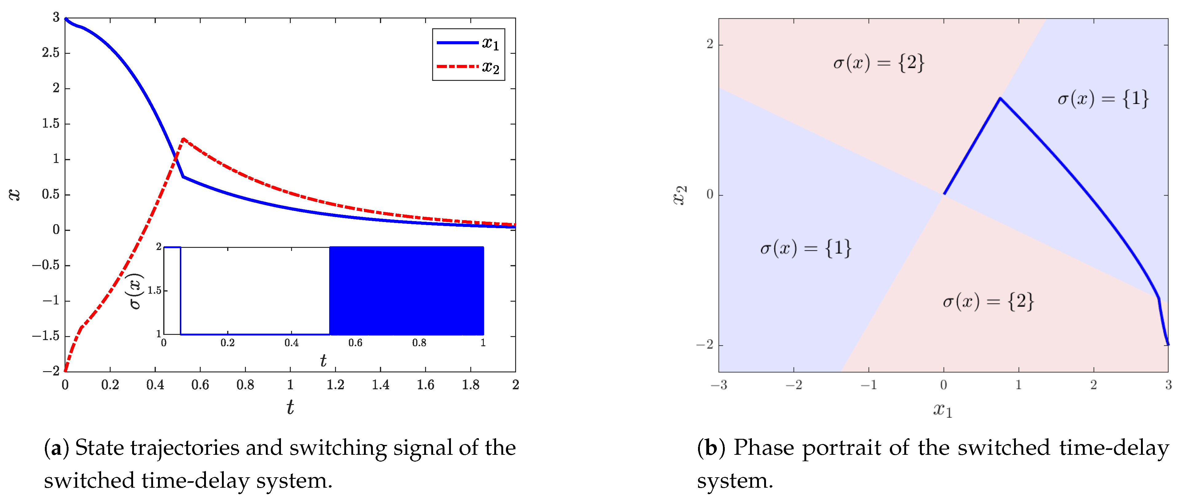
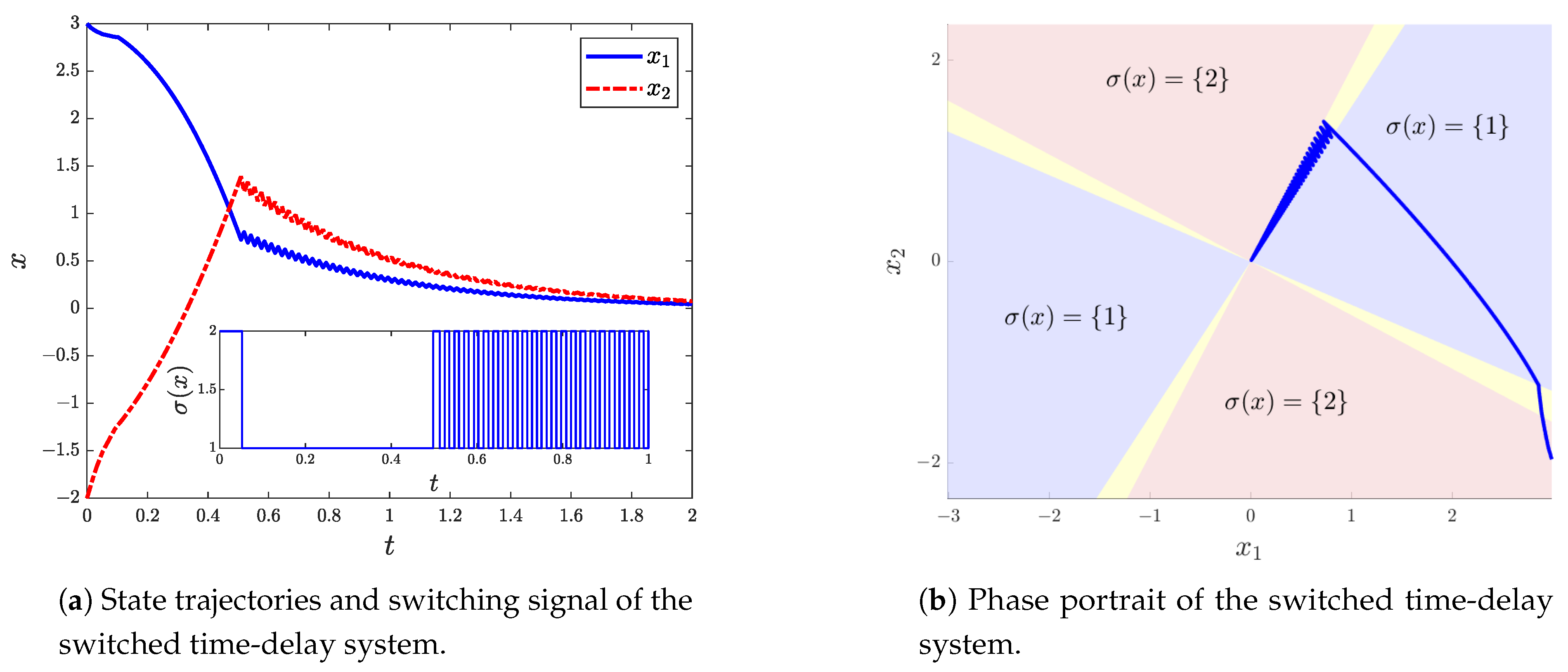
We next use this result to validate our switching strategy by a numercial simulation. Let the initial condition be $\phi \left(\theta \right)=[3-2]$, $\theta \in [-h,0]$, and $d\left(t\right)=0.014-0.014sin\left(t\right)$. Clearly, $\mu =0.014$ and $h=0.028$. The evolution of the switched time-delay system under the min-projection switching strategy (7) is depicted in Figure 1, in which it can be seen that the system enters a sliding mode and is asymptotically stable at origin. To avoid the occurrence of sliding motion, we next adopt the modified min-projection switching strategy and take $\varrho =0.8$. Figure 2 illustrates the evolution of the switched time-delay system under the modified min-projection switching strategy, from which the effectiveness of the modified min-projection switching strategy in preventing sliding motion is verified.

Example 2.

Consider a switched system with time varying delay in the form of (1) with

$$\begin{array}{cc}\hfill A_1& =\left[\begin{array}{ccc}\hfill -3& \hfill -2& \hfill 1\\ \hfill 1& \hfill 1& \hfill -1\\ \hfill 1& \hfill 0& \hfill 0\end{array}\right],B_1=\left[\begin{array}{ccc}\hfill 0& \hfill -4& \hfill 1\\ \hfill 1& \hfill 1& \hfill -2\\ \hfill 0& \hfill 0& \hfill -2\end{array}\right],\hfill \\ \hfill A_2& =\left[\begin{array}{ccc}\hfill -1& \hfill 1& \hfill 2\\ \hfill -2& \hfill -2& \hfill -1\\ \hfill -1& \hfill 2& \hfill -1\end{array}\right],B_2=\left[\begin{array}{ccc}\hfill 2& \hfill 2& \hfill 1\\ \hfill 1& \hfill -1& \hfill -2\\ \hfill 1& \hfill -2& \hfill -1\end{array}\right].\hfill \end{array}$$

By sweeping over the values of α, we find that there is no stable convex combination of $A_i+B_i$, $i\in I[1,2]$. Hence, the switching strategy proposed in [12,13,14] is not applicable to this system. On the other hand, the constrained optimization problem (34) is feasible when $J=2$. The calculated upper delay bounds for various values of μ are listed in

Table 2. Delay bound $h^{*}$ calculated for Example 2.

Methods	$\mathit{\mu }=0$	$\mathit{\mu }=0.1$	$\mathit{\mu }=0.5$
[12]	-	-	-
[13]	-	-	-
[14]	-	-	-
Theorem 1 ($J=2$)	0.0415	0.0337	0.0337

.

In particular, when $\mu =0.5$, we obtain from the two-step iterative algorithm that $h^{*}=0.0337$ and

$$\begin{array}{cccc}\hfill P_1& =\left[\begin{array}{ccc}\hfill 5.31& \hfill 11.10& \hfill -8.62\\ \hfill 11.10& \hfill 34.15& \hfill -29.76\\ \hfill -8.62& \hfill -29.76& \hfill 30.31\end{array}\right],\hfill & \hfill P_2& =\left[\begin{array}{ccc}\hfill 6.17& \hfill 7.75& \hfill -2.74\\ \hfill 7.75& \hfill 13.28& \hfill -8.81\\ \hfill -2.74& \hfill -8.81& \hfill 14.58\end{array}\right],\hfill \\ \hfill Q& =\left[\begin{array}{ccc}\hfill 3.68& \hfill 8.29& \hfill -3.31\\ \hfill 8.29& \hfill 20.79& \hfill -6.82\\ \hfill -3.31& \hfill -6.82& \hfill 12.61\end{array}\right],\hfill & \hfill U& =\left[\begin{array}{ccc}\hfill 3.57& \hfill 3.18& \hfill -2.93\\ \hfill 3.18& \hfill 15.21& \hfill -9.69\\ \hfill -2.93& \hfill -9.69& \hfill 6.45\end{array}\right],\hfill \\ \hfill X& =\left[\begin{array}{ccc}\hfill 7.20& \hfill 7.01& \hfill -6.45\\ \hfill 12.77& \hfill 15.93& \hfill -13.46\\ \hfill -8.91& \hfill -17.69& \hfill 13.20\end{array}\right],\hfill & \hfill R& =\left[\begin{array}{ccc}\hfill 1.24& \hfill 2.95& \hfill -1.89\\ \hfill 2.95& \hfill 7.00& \hfill -4.49\\ \hfill -1.89& \hfill -4.49& \hfill 2.88\end{array}\right]\times {10}^{-2},\hfill \\ \hfill W_{11}& =\left[\begin{array}{ccc}\hfill -0.84& \hfill -1.46& \hfill 0.01\\ \hfill -1.46& \hfill -8.70& \hfill -1.15\\ \hfill 0.01& \hfill -1.15& \hfill -19.21\end{array}\right]\times {10}^{-7},\hfill & \hfill W_{21}& =\left[\begin{array}{ccc}\hfill 1.75& \hfill 0.48& \hfill -0.35\\ \hfill 0.48& \hfill 1.77& \hfill -0.85\\ \hfill -0.35& \hfill -0.85& \hfill 1.10\end{array}\right],\hfill \\ \hfill Z& =\left[\begin{array}{ccc}\hfill 21.69& \hfill 22.20& \hfill -15.28\\ \hfill 22.20& \hfill 38.92& \hfill -30.45\\ \hfill -15.28& \hfill -30.45& \hfill 30.03\end{array}\right],\hfill & \hfill & \begin{array}{cc}{\alpha }_{11}=1,\hfill & {\alpha }_{21}=0,\hfill \\ {\beta }_{12}=1.1568,\hfill & {\beta }_{21}=0.5924,\hfill \\ {\eta }_{12}=0.0051,\hfill & {\eta }_{21}=0.0777.\hfill \end{array}\hfill \end{array}$$

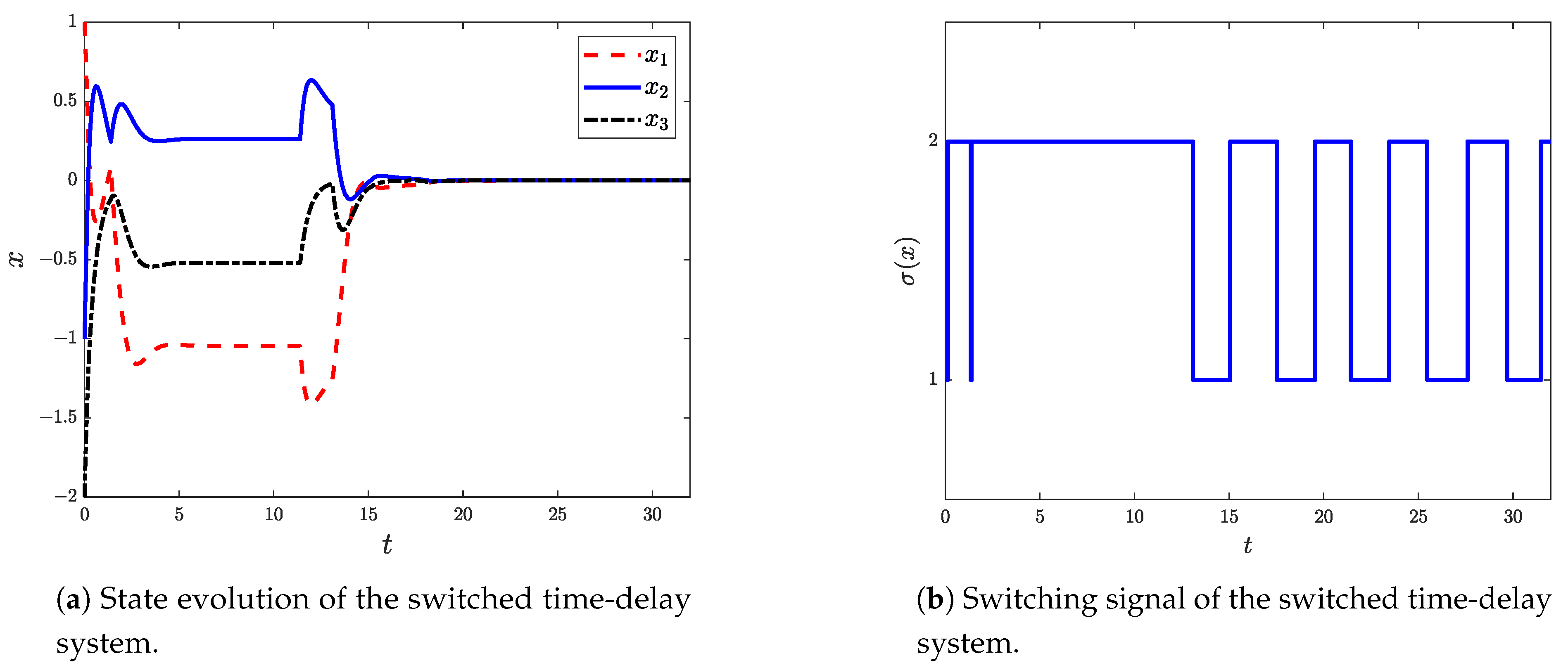
We next validate our switching strategy using this result. Let $d\left(t\right)=0.016+0.016sin\left(t\right)$. The state evolution of the switched time-delay system with the initial condition taken as $\phi \left(\theta \right)=[-322]$, $\theta \in [-h,0]$, is plotted in Figure 3. Clearly, the switched time-delay system is asymptotically stable at the origin under the min-projection switching strategy (7).

5. Conclusions and Future Work

In this paper, we studied the problem of stabilizing a switched time-delay linear system via a state-dependent switching strategy. We established that the min-projection switching strategy, originally designed for delay-free switched linear systems, is robust with respect to a small state delay. Compared to existing works, we imposed a less restrictive assumption on the considered system, and thus, our method could be applied to a larger class of switched systems. For systems satisfying the relaxed assumption, an algorithm was developed to estimate the upper bound of the tolerable time delay and a modified switching strategy was proposed to avoid the occurrence of sliding motion. Numerical examples verified our theoretical results.

In recent years, new bounding techniques for cross terms in (17) and (19) have emerged to derive less conservative stability criteria for linear systems with time-varying delays, e.g., [24,25,26,27]. Thus our future work will focus on (1) investigating how to incorporate these new techniques into the method we developed in this paper, and (2) conducting comparison studies on conservatism and computational complexity among these new techniques.

References

- Liberzon, D.; Morse, A.S. Basic problems in stability and design of switched systems. IEEE Control Syst. Mag. 1999, 19, 59–70. [Google Scholar]
- Lu, Y.; Zhang, W. A piecewise smooth control-Lyapunov function framework for switching stabilization. Automatica 2017, 76, 258–265. [Google Scholar] [CrossRef] [Green Version]
- Pettersson, S.; Lennartson, B. Stabilization of hybrid systems using a min-projectionstrategy. In Proceedings of the 2001 American Control Conference, Arlington, VA, USA, 25–27 June 2001; Volume 1, pp. 223–228. [Google Scholar]
- Dehghan, M.; Ong, C. Computations of mode-dependent dwell times for discrete-time switching system. Automatica 2013, 49, 1804–1808. [Google Scholar] [CrossRef]
- Xiang, W.; Xiao, J. Stabilization of switched continuous-time systems with all modes unstable via dwell time switching. Automatica 2014, 50, 940–945. [Google Scholar] [CrossRef]
- Kim, K.D.; Park, P.; Ko, J. Output-feedback H∞ control of systems over communication networks using a deterministic switching system approach. Automatica 2004, 64, 121–125. [Google Scholar] [CrossRef]
- Sun, X.; Zhao, J.; Hill, D.J. Stability and L2-gain analysis for switched delay systems: A delay-dependent method. Automatica 2006, 42, 1769–1774. [Google Scholar] [CrossRef]
- Wang, D.; Wang, W.; Shi, P. Delay-dependent exponential stability for switched delay systems. Optim. Control Appl. Methods 2009, 30, 383–397. [Google Scholar] [CrossRef]
- Vu, L.; Morgansen, K.A. Stability of Time-Delay Feedback Switched Linear Systems. IEEE Trans. Autom. Control 2010, 55, 2385–2390. [Google Scholar] [CrossRef]
- Zhai, G.; Chen, X.; Ikeda, M.; Yasuda, K. Stability and L2 gain analysis for a class of switched symmetric systems. In Proceedings of the 41st IEEE Conference on Decision and Control, Las Vegas, NV, USA, 10–13 December 2002; Volume 4, pp. 4395–4400. [Google Scholar]
- Zhang, W.A.; Yu, L. Stability analysis for discrete-time switched time-delay systems. Automatica 2009, 45, 2265–2271. [Google Scholar] [CrossRef]
- Kim, S.; Campbell, S.A.; Liu, X. Stability of a class of linear switching systems with time delay. IEEE Trans. Circuits Syst. I Regul. Pap. 2006, 53, 384–393. [Google Scholar]
- Sun, X.; Wang, W.; Liu, G.; Zhao, J. Stability Analysis for Linear Switched Systems With Time-Varying Delay. IEEE Trans. Syst. Man Cybern. Part B (Cybern.) 2008, 38, 528–533. [Google Scholar]
- Zhu, X.L.; Yang, H.; Wang, Y.; Wang, Y.L. New stability criterion for linear switched systems with time-varying delay. Int. J. Robust Nonlinear Control 2014, 24, 214–227. [Google Scholar] [CrossRef]
- Hu, T.; Ma, L.; Lin, Z. Stabilization of Switched Systems via Composite Quadratic Functions. IEEE Trans. Autom. Control 2008, 53, 2571–2585. [Google Scholar] [CrossRef]
- Hou, T.; Li, Y.; Lin, Z. An improved result on stabilization of switched linear systems with time-varying delay. In Proceedings of the IFAC Symposium on Time Delay Systems-16th TDS 2021, Guangzhou, China, 29 September–1 October 2021. [Google Scholar]
- Wicks, M.; De Carlo, R. Solution of coupled Lyapunov equations for the stabilization of multimodal linear systems. In Proceedings of the 1997 American Control Conference, Albuquerque, NM, USA, 6 June 1997; Volume 3, pp. 1709–1713. [Google Scholar]
- Subbotin, A. Generalized Solutions of First-Order PDEs: The Dynamical Optimization Perspective; Birkhäuser: Basel, Switzerland, 1994. [Google Scholar]
- Gu, K. An integral inequality in the stability problem of time-delay systems. In Proceedings of the 39th IEEE Conference on Decision and Control, Sydney, Australia, 12–15 December 2000; Volume 3, pp. 2805–2810. [Google Scholar]
- Park, P.; Ko, J.W.; Jeong, C. Reciprocally convex approach to stability of systems with time-varying delays. Automatica 2011, 47, 235–238. [Google Scholar] [CrossRef]
- Seuret, A.; Gouaisbaut, F. Wirtinger-based integral inequality: Application to time-delay systems. Automatica 2013, 49, 2860–2866. [Google Scholar] [CrossRef] [Green Version]
- Filippov, A.F. Differential Equations with Discontinuous Righthand Sides; Springer: Dordrecht, The Netherlands, 1988. [Google Scholar]
- Hassibi, A.; How, J.; Boyd, S. A path-following method for solving BMI problems in control. In Proceedings of the 1999 American Control Conference, San Diego, CA, USA, 2–4 June 1999; Volume 2, pp. 1385–1389. [Google Scholar]
- Chen, J.; Xu, S.; Zhang, B. Single/multiple integral inequalities with applications to stability analysis of time-delay systems. IEEE Trans. Autom. Control 2017, 62, 3488–3493. [Google Scholar] [CrossRef]
- Kim, J.H. Further improvement of Jensen inequality and application to stability of time-delayed systems. Automatica 2016, 40, 1205–1212. [Google Scholar]
- Seuret, A.; Liu, K.; Gouaisbaut, F. Generalized reciprocally convex combination lemmas and its application to time-delay systems. Automatica 2018, 85, 488–493. [Google Scholar] [CrossRef] [Green Version]
- Zhang, C.K.; Long, F.; He, Y.; Yao, W.; Jiang, L.; Wu, M. A relaxed quadratic function negative-determination lemma and its application to time-delay systems. Automatica 2020, 113, 108764. [Google Scholar] [CrossRef]
Figure 1.
Example 1: evolution of the switched system under the min-projection switching strategy (7).
Figure 2.
Example 1: evolution of the switched system under the modified min-projection switching strategy.
Figure 3.
Example 2: evolution of the switched system under the min-projection switching strategy (7).
Publisher’s Note: MDPI stays neutral with regard to jurisdictional claims in published maps and institutional affiliations. |
© 2021 by the authors. Licensee MDPI, Basel, Switzerland. This article is an open access article distributed under the terms and conditions of the Creative Commons Attribution (CC BY) license (https://creativecommons.org/licenses/by/4.0/).
Share and Cite
MDPI and ACS Style
Hou, T.; Li, Y.; Lin, Z. Stabilization of Switched Time-Delay Linear Systems through a State-Dependent Switching Strategy. Actuators 2021, 10, 261. https://0-doi-org.brum.beds.ac.uk/10.3390/act10100261
AMA Style
Hou T, Li Y, Lin Z. Stabilization of Switched Time-Delay Linear Systems through a State-Dependent Switching Strategy. Actuators. 2021; 10(10):261. https://0-doi-org.brum.beds.ac.uk/10.3390/act10100261
Chicago/Turabian StyleHou, Tan, Yuanlong Li, and Zongli Lin. 2021. "Stabilization of Switched Time-Delay Linear Systems through a State-Dependent Switching Strategy" Actuators 10, no. 10: 261. https://0-doi-org.brum.beds.ac.uk/10.3390/act10100261
Note that from the first issue of 2016, this journal uses article numbers instead of page numbers. See further details here.