Predefined-Time Control of Full-Scale 4D Model of Permanent-Magnet Synchronous Motor with Deterministic Disturbances and Stochastic Noises

Abstract

This paper presents a predefined-time convergent robust control algorithm that allows the control designer to set the convergence time in advance, independently of initial conditions, deterministic disturbances, and stochastic noises. The control law is consequently designed and verified by simulations for a full-scale 4-degrees-of-freedom (4D) permanent-magnet synchronous motor (PMSM) system in cases of a disturbance-free system with completely measurable states, a disturbance-free system with incompletely measurable states, a system with incompletely measurable states in the presence of deterministic disturbances, and a system with incompletely measurable states in the presence of both deterministic disturbances and stochastic noises. Numerical simulations are provided for the full-scale 4D PMSM system in order to validate the obtained theoretical results in each of the considered cases. To the best of our knowledge, this is the first attempt to design a predefined-time convergent control law for multi-dimensional systems with incompletely measurable states in the presence of both deterministic disturbances and stochastic noises.

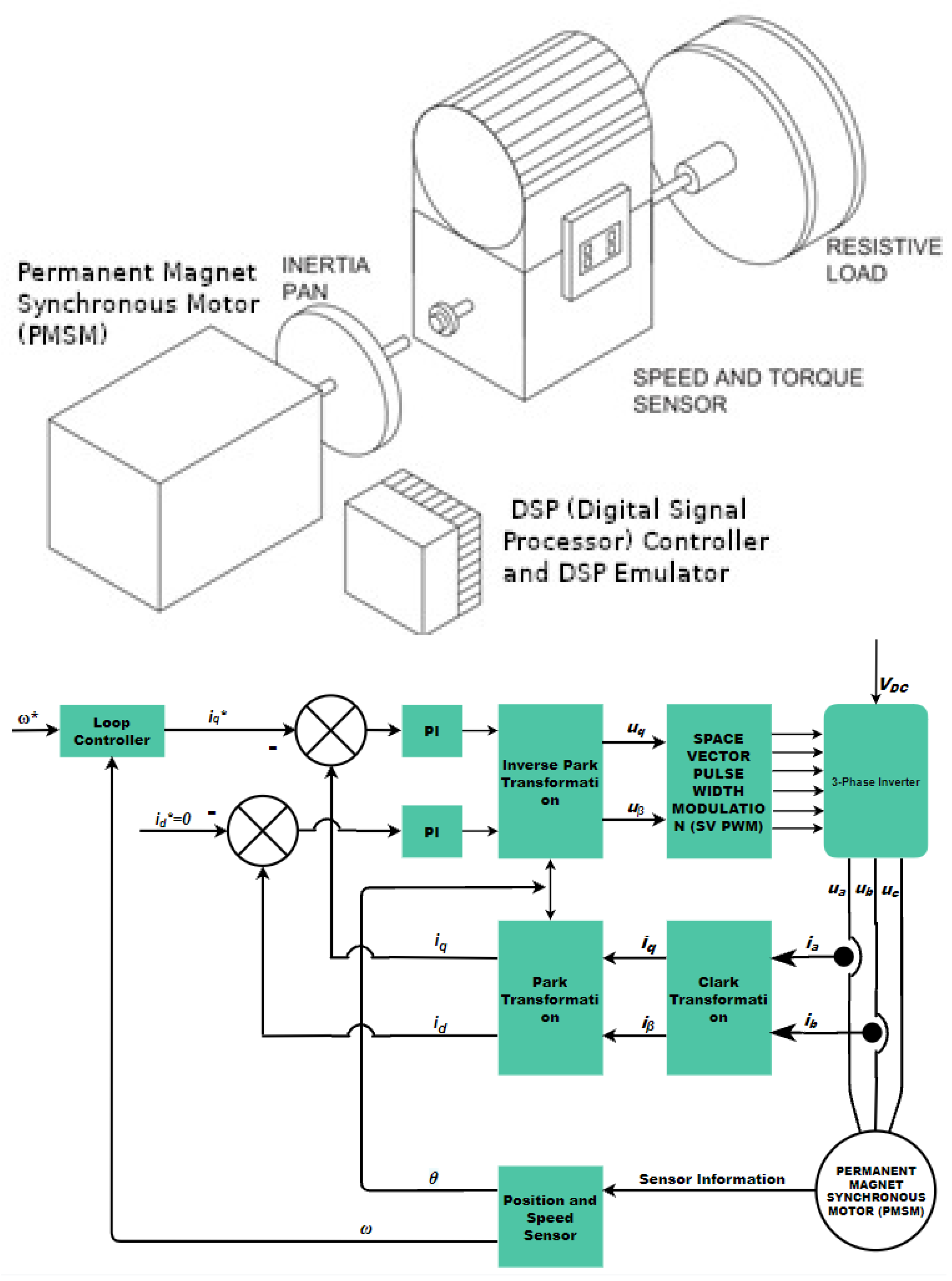
1. Introduction

A designer of control systems faces two problems [1,2] when trying to find a control algorithm to drive the system states to an equilibrium point. On the one hand, the designer must overcome the problem of convergence rate. On the other hand, he/she needs to solve the problem of robustness against disturbances, uncertainties, and noises affecting the system. In the linear control theory, it is relatively easy to solve the stated problems; however, when dealing with nonlinear systems, these two problems present a great challenge for the control theory community [3,4].

An important application of fast robust controllers is regulating permanent-magnet synchronous motors (PMSMs). PMSMs have many advantages in comparison to induction motors. They are more efficient—95–97% compared to 90–92% in typical induction motors—lighter, and smaller [5]. Furthermore, they generally have larger torques, higher rotation speeds, higher power densities, and quicker responses. All these characteristics make them perfectly suitable for applications in power trains of electrical vehicles [6], trains [7], industrial robots [8,9], unmanned autonomous vehicles [10], and others. Adaptive sensorless control laws for PMSMs of industrial robots are designed in [11,12], PMSM rotor position/speed estimators are proposed in [13,14], and a comprehensive review of various PMSM control techniques is provided in [15]. On the other hand, the PMSM performance might be adversely affected by uncertainties [16] and disturbances due to variations in external load [17], temperature, and/or magnetic saturation [18]. There are many techniques, including adaptive [19], model-predictive [20,21], and fault-tolerant ones [22,23], to counteract the disturbance influence. Therefore, a controller that is robust against disturbances, uncertainties, and noises, and also responds rapidly to the system requests, is in great demand.

Two solutions have been proposed to solve the convergence problem: finite- and fixed-time controllers (please see [24] for a detailed review). However, even though various algorithms have been developed using either method, the proposed solutions often suffer from the drawback that the finite convergence time unboundedly grows as the initial conditions increase or there is no convergence at all. On the other hand, although the convergence time of a fixed-time controller does not depend on the initial conditions, the designer can only calculate an upper estimate of the convergence time, which might be much larger than the real convergence time. For example, in [17], the calculated convergence time estimate is 7228 s, while the real convergence time is 114 s. Therefore, a control algorithm, whose performance is not affected by the initial conditions and also allows one to know precisely the true convergence time, is in great demand as well.

To eliminate the mentioned drawback of finite- and fixed-time controllers, a new technique, known as predefined-time control, has been proposed, whose key idea is to propose a control law that relates the state variables and the desired convergence time. For example, [25,26] have implemented exponential and polynomial forms of the control input that relate the variable states and the convergence time. Moreover, in [27], a control input in an exponential form has been employed for a multi-dimensional dynamical system. However, the foregoing control laws are proposed only for systems of degrees one or two [25,28], or the control magnitude exponentially grows for large values of negative initial conditions [27], as shown in [29].

In this paper, a predefined-time convergent control algorithm is proposed that allows the control designer to set the convergence time in advance, independently of initial conditions, deterministic disturbances, and stochastic noises. The control law is consequently designed and verified by simulations for a full-scale 4-degrees-of-freedom (4D) PMSM model [30] in cases of a disturbance-free system with completely measurable states, a disturbance-free system with incompletely measurable states where only the rotation angle can be measured, a system with incompletely measurable states in the presence of deterministic disturbances, and a system with incompletely measurable states in the presence of both deterministic disturbances and stochastic noises. The proposed algorithm is free from the restriction of exponential control magnitude growth and can be applied to multi-dimensional systems. To the best of our knowledge, this is the first attempt to design a predefined-time convergent control law for multi-dimensional systems with incompletely measurable states in the presence of both deterministic disturbances and stochastic noises. The numerical simulation results obtained for a full-scale 4D PMSM system show that the designed control law is capable of driving the PMSM system states to an equilibrium point for a pre-assigned time and operates with control magnitudes suitable for practical applications.

The paper is organized as follows. In Section 2, the predefined-time control problem is stated for a general nonlinear dynamical system and a full-scale 4D PMSM model is described. Section 3, Section 4, Section 5 and Section 6 consequently present implementations of the proposed predefined-time convergent control algorithm for a full-scale 4D PMSM model in all the above-mentioned cases. Some conclusions to this study are provided in Section 7.

2. Problem Statement

2.1. Predefined-Time Convergence

Before formally introducing the control problem for a full-scale 4D PMSM model, let us define the predefined-time convergence notion for a general nonlinear n-dimensional dynamic system.

$$\dot{x}\left(t\right)=u\left(t\right)+\xi \left(t\right)+\sigma (t,x\left(t\right))dW\left(t\right),x\left(t_0\right)=x_0,$$

(1)

where $x\left(t\right)\in R^n$ is the system state, $u\left(t\right)\in R^m$ is the control input, $\xi \left(t\right)$ is a deterministic disturbance satisfying the Lipschitz condition

$$\Vert \xi \left(t_1\right)-\xi \left(t_2\right)\Vert \le L\left|t_1-t_2\right|,$$

(2)

with a certain constant L. $W\left(t\right)$ is a Wiener process defined in the complete probability space $\left(\mathsf{\Omega },F,P\right)$, where $\mathsf{\Omega }$ is the sample space, F is a $\sigma$ field with a filtration ${\left\{F_t\right\}}_{\left(t\ge 0\right)}$, and P is a probability measure. The condition $\sigma \left(t,0\right)=0$ must be satisfied for all $t\ge t_0$.

The predefined-time convergence definitions are separately introduced for deterministic and stochastic systems [29].

• The system (1) is only affected by a deterministic disturbance—that is, $\sigma (t,x(t\left)\right)=0$. The predefined-time convergence is introduced for a deterministic system.

  Definition 1. Predefined-time convergence for a deterministic system

   

  The system (1) is called predefined-time convergent to the origin, if

  (a) 

  It is fixed-time convergent to the origin, i.e., for any initial state $x_0$, there exists a positive constant $T_{max}>0$, independent of $x_0$, such that $x\left(t\right)=0$ $\forall t\ge T_{max}$.

  (b) 

  $T_{max}$ is independent of any initial conditions and disturbances and can be arbitrarily chosen in advance.

  (c) 

  $T_{max}\ge T_f$, where $T_f$ is the true convergence time.

• The system (1) is affected by a deterministic disturbance and a stochastic noise—that is, $\sigma (t,x(t\left)\right)\ne 0$. The predefined-time convergence is introduced for a stochastic system.

  Definition 2. Predefined-time convergence for a stochastic system

   

  The system (1) is called predefined-time convergent to the origin in ρ-mean, if

  (a) 

  It is fixed-time convergent to the origin in ρ-mean, i.e., for any initial state $x_0$, there exists a positive constant $T_{max}>0$, independent of $x_0$, such that $E{\left[x\left(t\right)\right]}^{\rho }=0$, $\forall t\ge T_{max}$.

  (b) 

  $T_{max}$ is independent of any initial conditions and disturbances and can be arbitrarily chosen in advance.

  (c) 

  $T_{max}\ge T_f$, where $T_f$ is the true convergence time.

2.2. PMSM Predefined-Time Stabilization Problem

Let us consider the following full-scale 4D model of the permanent-magnet synchronous DC motor (PMSM), whose general view and model block diagram are shown in Figure 1. The model dynamics are governed by the following system of differential equations [30]:

$$\begin{array}{c}\dot{\theta }=\omega ,\hfill \\ \dot{\omega }=\frac{K_t}{J}{i}_q-\frac{B}{J}\omega -\frac{T_L}{L},\hfill \\ {\dot{i}}_d=-\frac{R_s}{L_d}{i}_d+n_p{\omega }_o{i}_q+\frac{u_d}{L_d},\hfill \\ {\dot{i}}_q=-\frac{R_s}{L_q}{i}_q-n_p{\omega }_o{i}_d-\frac{n_p{\varphi }_v\omega }{L_q}+\frac{u_q}{L_q}.\hfill \end{array}$$

(3)

Here, $\theta \left(t\right)$ is the rotation angle, $\omega \left(t\right)$ is the rotor speed, $i_d\left(t\right)$ and $i_q\left(t\right)$ are the d-axis and q-axis stator currents, $u_d$ (the control input) and $u_q$ are the d-axis and q-axis stator voltages, $T_L$ (uncoupled perturbation) is the load torque, $L_d$ and $L_q$ are the inductances of the d and q axes satisfying $L_d=L_q=L$, $R_s$ is the stator resistance, $n_p$ is the number of pole pairs, ${\varphi }_v$ is the rotor flux linkage, $K_T=\left(3n_p{\varphi }_v\right)/2$, J is the moment of inertia, ${\omega }_0$ is the initial rotor speed, and B is the viscous friction coefficient. The variables $\theta \left(t\right)$, $\omega \left(t\right)$, $i_q\left(t\right)$, and $i_d\left(t\right)$ are selected as system states to form a four-dimensional state vector.

The system in (3) can be transformed [17] into a chain of integrators. To do so, let us introduce new state variables $v_1\left(t\right)=\dot{\omega }$ and $v_2\left(t\right)={\dot{v}}_1$. After calculating the derivatives of $v_1\left(t\right)$ and $v_2\left(t\right)$ in view of Equation (3), the following system in the chain of integrators form is obtained:

$$\begin{array}{cc}\hfill \dot{\theta }=& \omega ,\hfill \\ \hfill \dot{\omega }=& v_1,\hfill \\ \hfill {\dot{v}}_1=& v_2,\hfill \\ \hfill \dot{v_2}=& v_1\left[-n_p^2{\omega }_o^2-\frac{R_{s}B}{J{L}_q}-\frac{R_s^2}{L_q{L}_d}-\frac{R_{s}B}{J{L}_d}-\frac{K_T{n}_p{\varphi }_v}{J{L}_q}\right]\hfill \\ \hfill & +T_L\left[-\frac{n_p^2{\omega }_0^2}{J}-\frac{R_S^2}{J{L}_q{L}_d}\right]+\omega \left[-\frac{n_p^2{\omega }_{0}B}{J}-\frac{R_s^2}{J{L}_q{L}_d}-\frac{K_T{R}_s{n}_p{\varphi }_v}{J{L}_q{L}_d}\right]\hfill \\ \hfill & +v_2\left[-\frac{R_S}{L_q}-\frac{R_S}{L_d}-\frac{B}{J}\right]+u_q\frac{K_T{R}_S}{J{L}_q{L}_d}-u_d\frac{K_T{n}_p{\omega }_0}{J{L}_d}.\hfill \end{array}$$

(4)

The PMSM predefined-time stabilization problem is to design a continuous control law that drives all the states of the system (4), including $\theta$ and $\omega$, to the origin for a predefined time, independently of state initial conditions, deterministic disturbances, and stochastic noises. The control law is consequently designed and verified by simulations for a full-scale 4D PMSM model in the following four cases.

• The system (4) is not affected by any disturbance, there is no noise entering the system, and all system states are measurable. A predefined-time convergent control law must be employed to drive all the states of the system (4) to the origin.
• The system (4) is not affected by any disturbance or noise; however, only the state variable $\theta$ can be measured. In this case, a predefined-time convergent observer must be employed to reconstruct the other three state variables.
• The system (4) is affected by a deterministic disturbance, and only the state variable $\theta$ can be measured. In this case, a predefined-time convergent compensator must be employed to estimate the disturbance.
• The system (4) is affected by a deterministic disturbance and a stochastic noise, and only the state variable $\theta$ can be measured. In this case, a predefined-time convergent control law must be specialized for stochastic systems.

The corresponding algorithms are designed in the following sections.

3. PMSM Predefined-Time Stabilization for Completely Measured States

3.1. Control Design

In this section, a predefined time-convergent control law is designed for the system (4) with completely measured states without disturbances and noise. The full-scale 4D PMSM model takes the form

$$\begin{array}{ccc}\hfill \dot{\theta }& \hfill =\hfill & \omega ,\hfill \\ \hfill \dot{\omega }& \hfill =\hfill & v_1,\hfill \\ \hfill {\dot{v}}_1& \hfill =\hfill & v_2,\hfill \\ \hfill {\dot{v}}_2& \hfill =\hfill & K_1{v}_1+K_2\omega +K_3{v}_2-K_4{u}_d,\hfill \end{array}$$

(5)

where

$$\begin{array}{c}{K}_1=-n_p^2{\omega }_o^2-\frac{R_{s}B}{J{L}_q}-\frac{R_S^2}{L_q{L}_d}-\frac{R_{s}B}{J{L}_d}-\frac{K_T{n}_p{\varphi }_v}{J{L}_q},\hfill \\ K_2=-\frac{n_p^2{\omega }_{o}B}{J}-\frac{R_s^2}{J{L}_q{L}_d}-\frac{K_T{R}_s{n}_p{\varphi }_v}{J{L}_q{L}_d},\hfill \\ K_3=-\frac{R_s}{L_q}-\frac{R_s}{L_d}-\frac{B}{J},\hfill \\ K_4=\frac{K_T{n}_p{\omega }_o}{J{L}_d}\hfill & & \hfill \end{array}$$

(6)

The following control law is proposed:

$$\begin{array}{c}\hfill u_d\left(t\right)=\left\{\begin{array}{c}\frac{1}{K_4}\left(z_3+K_1{v}_1+K_2\omega +K_3{v}_2-\frac{\partial v_{2d}}{\partial \theta }\left(z_2-{\psi }_1\right)\right.\hfill \\ \left.-\frac{\partial v_{2d}}{\partial z_2}\left(z_3-{\psi }_2-\theta \right)-\frac{\partial v_{2d}}{\partial z_3}\left(z_4-z_2-{\psi }_3\right)-\frac{\partial v_{2d}}{\partial t}+{\psi }_4\right),\hfill & 0<t\le t_f,\hfill \\ 0,\hfill & t>t_f,\hfill \end{array}\right.\end{array}$$

(7)

The control input $u_d\left(t\right)$ can be represented as $u_d\left(t\right)=u_{d1}\left(t\right)+u_{d2}\left(t\right)$, where

$$u_{d1}\left(t\right)=\frac{1}{K_4}\left(K_1{v}_1+K_2\omega +K_3{v}_2\right),$$

(8)

which opposes the known terms of the last equation in (5), and

$$u_{d2}\left(t\right)=\frac{1}{K_4}\left(z_3-\frac{\partial v_{2d}}{\partial \theta }\left(z_2-{\psi }_1\right)-\frac{\partial v_{2d}}{\partial z_2}\left(z_3-{\psi }_2-\theta \right)-\frac{\partial v_{2d}}{\partial z_3}\left(z_4-z_2-{\psi }_3\right)-\frac{\partial v_{2d}}{\partial t}+{\psi }_4\right),$$

(9)

which provides the predefined-time convergence of the states of the system (5) to the origin, as stated in the following theorem.

Theorem 1.

The control law (7) drives all the states of the system (5) to the origin within a predefined time $t_f$, and they remain there for any $t\ge t_f$.

Proof. 

The design of $u_{d2}\left(t\right)$ follows an approach similar to that in [27]. First, consider that the control law

$$u\left(t\right)=-{\eta }_1\frac{\left(e^{\left|\theta \right|}-1\right)}{e^{\left|\theta \right|}\left(t_f-t\right)}sign\left(\theta \right),$$

(10)

${\eta }_1>1$, makes the system

$$\dot{\theta }=u\left(t\right)$$

convergent to the origin for a predefined time $t_f$, as shown in [29]. Second, using the backstepping technique, it can be shown that all the states of the system (5) converge to the origin within the predefined time $t_f$. Defining the variables

$$\begin{array}{c}{\psi }_1=-{\eta }_1\frac{\left(e^{\left|\theta \right|}-1\right)}{e^{\left|\theta \right|}\left(t_f-t\right)}sign\left(\theta \right),\hfill \\ {\psi }_2=-{\eta }_2\frac{\left(e^{\left|z_2\right|}-1\right)}{e^{\left|z_2\right|}\left(t_f-t\right)}sign\left(z_2\right),\hfill \\ {\psi }_3=-{\eta }_3\frac{\left(e^{\left|z_3\right|}-1\right)}{e^{\left|z_3\right|}\left(t_f-t\right)}sign\left(z_3\right),\hfill \\ {\psi }_4=-{\eta }_4\frac{\left(e^{\left|z_4\right|}-1\right)}{e^{\left|z_4\right|}\left(t_f-t\right)}sign\left(z_4\right),\hfill \\ z_2=\omega -{\omega }_d,\mathrm{where}{\omega }_d(\theta ,t)=-{\psi }_1,\hfill \\ z_3=v_1-v_{1d},\mathrm{where}{v}_{1d}\left(\theta ,z_2,t\right)=-\theta -\frac{\partial {\psi }_1}{\partial t}-\left(z_2-{\psi }_1\right)\frac{\partial {\psi }_1}{\partial x_1}-{\psi }_2,\hfill \\ z_4=v_2-v_{2d},\mathrm{where}{v}_{2d}\left(\theta ,z_2,z_3,t\right)=-z_2+\omega \frac{\partial v_{1d}}{\partial \theta }+\frac{\partial v_{1d}}{\partial z_2}\left(z_3-{\psi }_2-\theta \right)+\frac{\partial v_{1d}}{\partial t}-{\psi }_3,\hfill \end{array}$$

(11)

and taking the time derivatives of $z_2$, $z_3$, and $z_4$, we obtain:

$$\begin{array}{cc}\hfill & {\dot{z}}_2=\dot{\omega }-{\dot{\omega }}_d=v_1+\frac{\partial {\omega }_d}{\partial \theta }\dot{\theta }+\frac{\partial {\omega }_d}{\partial t},\hfill \\ \hfill & {\dot{z}}_3={\dot{v}}_1-{\dot{v}}_{1d}=v_2-\left(\frac{\partial v_{1d}}{\partial \theta }\dot{\theta }+\frac{\partial v_{1d}}{\partial z_2}{\dot{z}}_2+\frac{\partial v_{1d}}{\partial t}\right),\hfill \\ \hfill & {\dot{z}}_4={\dot{v}}_2-{\dot{v}}_{2d}=u_d-\left(\frac{\partial v_{2d}}{\partial \theta }\dot{\theta }+\frac{\partial v_{2d}}{\partial z_2}{\dot{z}}_2+\frac{\partial v_{2d}}{\partial z_3}{\dot{z}}_3+\frac{\partial v_{2d}}{\partial t}\right).\hfill \end{array}$$

To prove the theorem, we need to find a Lyapunov function $V\left(t\right)$ that converges to zero for the predefined time $t_f$. To do so, the recursive Lyapunov functions are defined as follows:

$$\begin{array}{cc}& V_1\left(x_1\right)={\theta }^2\left(t\right),\hfill \\ & V_2\left(x_1,z_2\right)=V_1+z_2^2,\hfill \\ & V_3\left(x_1,z_2,z_3\right)=V_2+z_3^2,\hfill \\ & V_4\left(x_1,z_2,z_3,z_4\right)=V_3+z_4^2,\mathrm{which}\mathrm{yields}\hfill \\ & {\dot{V}}_4=2\theta \dot{\theta }+2z_2{\dot{z}}_2+2z_3{\dot{z}}_3+2z_4{\dot{z}}_4.\hfill & \end{array}$$

Substituting $\dot{\theta }$, ${\dot{z}}_2$, ${\dot{z}}_3$, and ${\dot{z}}_4$ into the last equation, we obtain

$${\dot{V}}_4=-2\theta {\psi }_1-2z_2{\psi }_2-2z_3{\psi }_3+2z_3{z}_4+2z_4\left[u_d-\left(\frac{\partial v_{2d}}{\partial \theta }\dot{\theta }+\frac{\partial v_{2d}}{\partial z_2}{\dot{z}}_2+\frac{\partial v_{2d}}{\partial z_3}{\dot{z}}_3+\frac{\partial v_{1d}}{\partial t}\right)\right].$$

Taking into account the expression for $u_d$ in (7) yields

$$\begin{array}{cc}\hfill {\dot{V}}_4=& -2\theta {\psi }_1-2z_2{\psi }_2-2z_3{\psi }_3-2z_4{\psi }_4\le -\frac{2{\eta }_1\left|\theta \right|\left(e^{\left|\theta \right|}-1\right)}{e^{\left|\theta \right|}\left(t_f-t\right)}-\hfill \\ & \frac{2{\eta }_2\left|z_2\right|\left(e^{\left|z_2\right|}-1\right)}{e^{\left|z_2\right|}\left(t_f-t\right)}-\frac{2{\eta }_3\left|z_3\right|\left(e^{\left|z_3\right|}-1\right)}{e^{\left|z_3\right|}\left(t_f-t\right)}-\frac{2{\eta }_4\left|z_4\right|\left(e^{\left|z_4\right|}-1\right)}{e^{\left|z_4\right|}\left(t_f-t\right)}.\hfill \end{array}$$

(12)

Since $V_4={\theta }^2+z_2^2+z_3^2+z_4^2$, then

$$V_4\le 4{\left(max\left\{\left|\theta \right|,\left|z_2\right|,\left|z_3\right|,\left|z_4\right|\right\}\right)}^2\mathrm{and}\sqrt{\frac{V_4}{4}}\le max\left\{\left|\theta \right|,\left|z_2\right|,\left|z_3\right|,\left|z_4\right|\right\}.$$

Using the last inequality, the expression (12) for ${\dot{V}}_4$, and the fact that the function $\frac{\left(e^{\left|z\right|}-1\right)}{e^{\left|z\right|}}$ is non-decreasing in z implies that

$${\dot{V}}_4\le -\frac{2\eta \sqrt{\frac{V_4}{4}}\left(e^{\sqrt{\frac{V_4}{4}}}-1\right)}{e^{\sqrt{\frac{v_4}{4}}}\left(t_f-t\right)},$$

(13)

where $\eta =min\left\{{\eta }_1,{\eta }_2,{\eta }_3,{\eta }_4\right\}$. Making the change of variables $\zeta =\sqrt{\frac{V_4}{4}}$ yields $\dot{\zeta }=\frac{{\dot{V}}_4}{8\zeta }$. Substituting this result into $\dot{V}$, we obtain

$$\dot{\zeta }\le -\frac{{\eta }^{\prime }\left(e^{\zeta }-1\right)}{e^{\zeta }\left(t_f-t\right)},$$

where ${\eta }^{\prime }=\frac{\eta }{4}$.

Since the last inequality presents a particular case of the differential inequality

$$\dot{\zeta }\le -\frac{{\eta }^{\prime }\left(e^{\left|\zeta \right|}-1\right)}{e^{\left|\zeta \right|}\left(t_f-t\right)}sign\left(\zeta \right)$$

(14)

for positive $\zeta$, which is dominated from the above by the differential equation following (10), its solution $\zeta \left(t\right)$ converges to zero for the predefined time $t_f$ and remains there afterwards, as shown in [29]. Therefore, the Lyapunov function $V_4$ converges to zero for the predefined time $t_f$ and remains there afterwards as well. This finally implies that all the states of the system (5) converge to zero for the predefined time $t_f$ and remain there for any $t\ge t_f$. □

3.2. PMSM Simulations

To verify the performance of the proposed control law (7), numerical simulations were run for the system (5) in MatLab 2020a, using the PMSM parameter values given in

Table 1. PMSM parameter values.

Variable	Value	Unit
$n_p$	4
$R_s$	$0.01$	$\mathsf{\Omega }$
$L_q$	$0.1$	$\mathrm{H}$
$L_d$	$0.1$	$\mathrm{H}$
$B$	$7.403\times {10}^{-5}$	$\mathrm{N}·\mathrm{m}·\mathrm{s}/\mathrm{rad}$
J	$1.74\times {10}^4$	$\mathrm{kg}·{\mathrm{m}}^2$
${\varphi }_v$	$0.1167$	$\mathrm{wb}$
$K_T$	$0.7002$
${\omega }_o$	1	$\mathrm{rpm}$
$t_f$	10	$\mathrm{s}$
$\eta$	$\left[20,20,20,20\right]$
$x_0$	$\left[-0.5,-3,-3,-5\right]$

.

Figure 2 shows that the control (7) drives all the states of the full-scale 4D PMSM system to the origin within the predefined time of 20 s. The zoom in Figure 2 demonstrates that the obtained predefined-time convergence satisfies the Levant’s test [31], with the precision up to ${10}^{-12}$, provided that the discretization step is set to ${10}^{-3}$ and the system dimension $n=4$. Moreover, it can be observed from Figure 3 that the magnitude of the control input remains within values acceptable in practice. Note, however, that the control input magnitudes presented in the given figures correspond to specific initial conditions and final times and evidently depend on both of these parameters. The same observation is valid for the simulations in subsequent sections.

4. PMSM Predefined-Time Stabilization for Incompletely Measured States

4.1. Observer Design

In the preceding section, all the states of the full-scale 4D PMSM system are assumed available; that is, there are sensors to measure the shaft angle, the angular velocity, and the currents. However, in practice, this is not always possible. Therefore, we need to reconstruct unmeasurable states. In this case, we have to use a predefined-time convergent observer to estimate unmeasurable states and then design a predefined-time convergent controller based on the obtained estimates. The corresponding problem is represented by the following system:

$$\begin{array}{cc}\hfill \dot{\theta }=& \omega ,\hfill \\ \hfill \dot{\omega }=& v_1,\hfill \\ \hfill {\dot{v}}_1=& v_2,\hfill \\ \hfill {\dot{v}}_2=& v_1\left[-n_p^2{\omega }_0^2-\frac{R_{S}B}{J{L}_q}-\frac{R_s^2}{L_q{L}_d}-\frac{R_{S}B}{J{L}_d}-\frac{K_T{n}_p{\varphi }_v}{J{L}_q}\right]\hfill \\ & +\omega \left[-\frac{n_p^2{\omega }_{0}B}{J}-\frac{R_S^2}{J{L}_q{L}_d}-\frac{K_T{R}_s{n}_p{\varphi }_v}{J{L}_q{L}_d}\right]\hfill \\ & +v_2\left[-\frac{R_S}{L_q}-\frac{R_S}{L_d}-\frac{B}{J}\right]-u_d\frac{K_T{n}_p{\omega }_0}{J{L}_d},\hfill \\ \hfill y=& \theta \left(t\right),\hfill \end{array}$$

(15)

where $y\left(t\right)$ is the only measured system output. The states $\omega ,v_1,v_2$ should be estimated by using a predefined-time observer to be able to proceed to the design of a predefined-time controller. For this purpose, the predefined-time convergent observer proposed in [32] is employed

$$\begin{array}{cc}\dot{\widehat{\theta }}=\hfill & \widehat{\omega }-\gamma k_{1}sign(\widehat{\theta }-y)\left({\displaystyle |}\widehat{\theta }{-y{\displaystyle |}}^{{\alpha }_1}+{{\displaystyle |}\widehat{\theta }-y{\displaystyle |}}^{{\beta }_1}\right),\hfill \\ \dot{\widehat{\omega }}=\hfill & {\widehat{v}}_1-{\gamma }^2{k}_{2}sign(\widehat{\theta }-y)\left({\displaystyle |}\widehat{\theta }{-y{\displaystyle |}}^{{\alpha }_2}+{{\displaystyle |}\widehat{\theta }-y{\displaystyle |}}^{{\beta }_2}\right),\hfill \\ {\dot{\widehat{v}}}_1=\hfill & {\widehat{v}}_2-{\gamma }^3{k}_{3}sign(\widehat{\theta }-y)\left({\displaystyle |}\widehat{\theta }{-y{\displaystyle |}}^{{\alpha }_3}+{{\displaystyle |}\widehat{\theta }-y{\displaystyle |}}^{{\beta }_3}\right),\hfill \\ {\dot{\widehat{v}}}_2=\hfill & -{\gamma }^4{k}_{4}sign(\widehat{\theta }-y)\left({\displaystyle |}\widehat{\theta }{-y{\displaystyle |}}^{{\alpha }_4}+{{\displaystyle |}\widehat{\theta }-y{\displaystyle |}}^{{\beta }_4}\right),\hfill \end{array}$$

(16)

where $\widehat{\theta }$, $\widehat{\omega }$, ${\widehat{v}}_1$, and ${\widehat{v}}_2$ are the estimates for the states $\theta$, $\omega$, $v_1$, and $v_2$, respectively. The values of $\alpha$, $\beta$, and $\gamma$ are assigned as

$$\begin{array}{ccc}{\alpha }_i\hfill & \hfill =\hfill & i\alpha -(i-1),\alpha \in \left[1-{ϵ}_1,1\right],\mathrm{for}\mathrm{a}\mathrm{sufficiently}\mathrm{small}{ϵ}_1>0,i=1,\dots ,4,\hfill \\ {\beta }_i\hfill & \hfill =\hfill & i\beta -(i-1),\beta \in \left[1,1+{ϵ}_2\right],\mathrm{for}\mathrm{a}\mathrm{sufficiently}\mathrm{small}{ϵ}_2>0i=1,\dots ,4,\hfill \\ \gamma \hfill & \hfill =\hfill & \ge 1,\hfill \end{array}$$

and the gains $k_1$, $k_2$, $k_3$, $k_4$ are selected such that the matrix

$$K=\left[\begin{array}{cccc}-k_1& 1& 0& 0\\ -k_2& 0& 1& 0\\ -k_3& 0& 0& 1\\ -k_4& 0& 0& 0\end{array}\right].$$

(17)

is Hurwitz.

It can be verified that the assumptions of Theorem 3 in [32] hold. Therefore, the convergence time of the observer (16) is bounded by the expression:

$$T\le \frac{4}{\gamma }\left(\frac{1}{1-\alpha }+\frac{1}{\beta -1}\right).$$

(18)

In this case, the proposed control law for the system (15) has a structure identical to (7), where the state variables are replaced by their estimates produced by the observer (16):

$$\begin{array}{c}\hfill u_d\left(t\right)=\left\{\begin{array}{c}\frac{1}{K_4}\left({\widehat{z}}_3+K_1{\widehat{v}}_1+K_2\widehat{\omega }+K_3{\widehat{v}}_2-\frac{\partial {\widehat{v}}_{2d}}{\partial \widehat{\theta }}\left({\widehat{z}}_2-{\widehat{\psi }}_1\right)\right.\hfill \\ \left.-\frac{\partial {\widehat{v}}_{2d}}{\partial {\widehat{z}}_2}\left({\widehat{z}}_3-{\widehat{\psi }}_2-\widehat{\theta }\right)-\frac{\partial {\widehat{v}}_{2d}}{\partial {\widehat{z}}_3}\left({\widehat{z}}_4-{\widehat{z}}_2-{\widehat{\psi }}_3\right)-\frac{\partial {\widehat{z}}_{2d}}{\partial t}+{\widehat{\psi }}_4\right),\hfill & 0<t\le t_f,\hfill \\ 0,\hfill & t>t_f.\hfill \end{array}\right.\end{array}$$

(19)

Simulation results corresponding to this control input are presented in the next subsection.

4.2. PMSM Simulations

To verify the performance of the proposed controller, numerical simulations are run for the system (15) and (16) in MatLab 2020a, using the values given in Table 1 and $\alpha =0.9$, $\beta =1.1$, $\gamma =10$, and $K=\left[4,6,4,1\right]$. According to (18) and the selected values of $\alpha$ and $\beta$, the predefined convergence time of the observer is calculated equal to 4 s. Note that the predefined convergence time for the observer is equal to 4 s, whereas the predefined convergence times for the corresponding controllers in this and subsequent sections are set to 10 or 20 s, so the controllers can work sufficiently long after the observer converges.

Figure 4 shows that the control (7) drives all the states of the full-scale 4D PMSM system to the origin within the predefined time of 20 s. The upper zoom in Figure 4 verifies that the estimates produced by the observer (16) converge to the real state values for less than 0.5 s. The second zoom in Figure 4 demonstrates that the obtained predefined-time convergence satisfies the Levant’s test [31], with the precision up to ${10}^{-12}$ virtually, provided that the discretization step is set to ${10}^{-3}$ and the system dimension $n=4$. Additionally, it can be observed from Figure 5 that the magnitude of the control input remains within values acceptable in practice.

5. PMSM Predefined-Time Stabilization for Incompletely Measured States with Deterministic Disturbances

5.1. Control Design

In the preceding sections, the full-scale 4D PMSM system was considered without deterministic disturbances or stochastic noises. Nonetheless, deterministic disturbances are common in practice and can appear, for instance, due to torque volatility or stator voltage supply failure. Let us consider the full-scale 4D PMSM system dynamics subject to deterministic disturbances

$$\begin{array}{ccc}\hfill \dot{\theta }& \hfill =\hfill & \omega ,\hfill \\ \hfill \dot{\omega }& \hfill =\hfill & v_1,\hfill \\ \hfill {\dot{v}}_1& \hfill =\hfill & v_2,\hfill \\ \hfill {\dot{v}}_2& \hfill =\hfill & K_1{v}_1+K_2\omega +K_3{v}_2-K_4{u}_d+K_5{u}_q,\hfill \\ \hfill y& \hfill =\hfill & \theta \hfill \end{array}$$

(20)

where the coefficients $K_1$, $K_2$, $K_3$, $K_4$ are defined in (6), the term $\xi \left(t\right)=K_5{u}_q$ is a disturbance satisfying the Lipschitz condition with constant L, and $K_5=\frac{K_T{R}_s}{J{L}_d{L}_q}$. The objective is to design a continuous control law that drives all the states of the system (20) to the origin for a predefined time, independently of state initial conditions, and maintains it there afterwards in spite of deterministic disturbances.

The control input solving this problem consists of two parts. The first nominal part, $u_{nom}$, drives the system (20) to the origin for a predefined time $t\le t_f$. This part is active only until $t=t_f$. The second compensator part, $v\left(t\right)$, compensates for deterministic disturbances, driving the system to the nominal track, and maintains the system (20) at the origin for $t\ge t_f$. The corresponding result is presented in the next theorem for the full-scale 4D PMSM system with completely measured states. If the states of the PMSM system are not completely measurable, the observer (16) and the control input based on the estimates produced by the observer are employed.

The following control law is proposed:

$$u\left(t\right)=\left\{\begin{array}{cc}{u}_d\left(t\right)+v\left(t\right)\hfill & 0,\le t<t_f,\hfill \\ v\left(t\right),\hfill & t_f\le t,\hfill \end{array}\right.$$

(21)

where the nominal control law $u_d$ is defined in (7) and

$$\begin{array}{c}\hfill v\left(t\right)=-{\lambda }_1{\left|s\left(t\right)\right|}^{\frac{1}{2}}\mathrm{sign}\left(s\left(t\right)\right)-{\lambda }_2{\left|s\left(t\right)\right|}^p\mathrm{sign}\left(s\left(t\right)\right)-{\alpha }_s{\int }_0^{t}sign\left(s\left(t\right)\right)ds\\ -\eta \frac{\left(e^{\left|s\right(t\left)\right|}-1\right)}{e^{\left|s\right(t\left)\right|}\left(t_f-t\right)}sign\left(s\left(t\right)\right).\hfill \end{array}$$

(22)

Here, $s\left(t\right)=v_2-r\left(t\right),\dot{r}\left(t\right)=u_{d2}\left(t\right)-v\left(t\right)$. Moreover, ${\lambda }_1,{\alpha }_s>0,{\lambda }_2\ge 0,\eta >1$ and $p>1$.

Theorem 2.

The control law (21) and (22) drives all the states of the system (20) to the origin for a predefined time and maintains them there for $t\ge t_f$ in the presence of a deterministic disturbance that satisfies the Lipschitz condition with constant L, if the following conditions hold: $\eta >1$, ${\alpha }_s>L$, ${\lambda }_1>\sqrt{2\alpha }$, ${\lambda }_2\ge 0$, and $p>1$.

Proof. 

According to Theorem 2 in [29], the given conditions ensure the predefined-time convergence of the variable $s\left(t\right)$ to zero, which results in $s\left(t\right)=\dot{s}\left(t\right)=0$ afterwards. Since $\dot{s}\left(t\right)={\dot{v}}_2\left(t\right)-\dot{r}\left(t\right)$, then $0={\dot{v}}_2\left(t\right)-\dot{r}\left(t\right)=u_{d2}\left(t\right)+\xi \left(t\right)-u_{d2}\left(t\right)+v\left(t\right)$, which leads to $v\left(t\right)=-\xi \left(t\right)$, so that $v\left(t\right)$ compensates for the disturbance $\xi \left(t\right)$. After compensating for the disturbance $\xi \left(t\right)$, the nominal control law $u_d$ provides the predefined-time convergence of all the states of the system (20) to the origin, according to Theorem 1 of Section 3. Since the compensation $v\left(t\right)=-\xi \left(t\right)$ also holds for $t\ge t_f$, all the states of the system (20) remain at the origin after their convergence as well. □

5.2. PMSM Simulations

To verify the performance of the proposed control law (21) and (22) in the presence of deterministic disturbances, numerical simulations were run for the system (20) in MatLab 2020a, using the same first nine PMSM parameter values as those in Table 1. The deterministic disturbance was selected as $u_q=0.1t+0.001\cos \left(10t\right)$, and the value of the coefficient $K_5$ was calculated according to the PMSM parameter values as $K_5=4024.14$. Accordingly, the Lipschitz constant was set to $L=443$. The newly assigned PMSM parameter values are listed in

Table 2. PMSM parameter values.

Variable	Value	Unit
$t_f$	20	$\mathrm{s}$
$\eta$	$\left[10,10,10,10\right]$
K	$\left[4,6,4,1\right]$
$x_0$	$\left[-0.5,-10,-40,-60\right]$
$\alpha$	$0.9$
$\beta$	$1.1$
$\gamma$	10
${\lambda }_1$	50
${\lambda }_2$	1
${\alpha }_s$	445

.

It is assumed that only the variable $\theta$ can be measured. Therefore, the observer (16) is used to reconstruct the unmeasured state variables, and the applied control input (21) and (22) is based on the estimates produced by the observer.

Figure 6 shows that the control input (21) and (22), based on the estimates produced by the observer (16), drives all the states of the full-scale 4D PMSM system to the origin within the predefined time of 20 s, with the precision ${10}^{-4}$, even for high disturbance magnitudes of order ${10}^3$. It can be observed from Figure 7 that the magnitude of the nominal control input $u_{d2}$ is higher than that without disturbances but still remains acceptable. Note that the obtained results provide better convergence precision and a lesser control magnitude than those presented in [17] for close values of the PMSM parameters and deterministic disturbances.

Finally, Figure 8 displays the compensator control input (22) $v\left(t\right)$, based on the estimates produced by the observer (16), against the disturbance $\xi \left(t\right)=K_5{u}_q=4024.14(0.1t+0.001\cos \left(10t\right))$. It can be observed that the control input $v\left(t\right)$ reliably compensates for the disturbance soon after the initial time moment.

6. PMSM Predefined-Time Stabilization with Incompletely Measured States with Deterministic Disturbances and Stochastic Noises

6.1. Control Design

In this section, the full-scale 4D PMSM system is considered with both deterministic disturbances and stochastic noises. As is known, stochastic noises are also common in practice and can appear, for instance, due to electromagnetic static or parasitic impulses. The full-scale 4D PMSM system dynamics subject to deterministic disturbances and stochastic noises are given by the equations

$$\begin{array}{ccc}\hfill \dot{\theta }& \hfill =\hfill & \omega ,\hfill \\ \hfill \dot{\omega }& \hfill =\hfill & v_1,\hfill \\ \hfill {\dot{v}}_1& \hfill =\hfill & v_2,\hfill \\ \hfill {\dot{v}}_2& \hfill =\hfill & K_1{v}_1+K_2\omega +K_3{v}_2-K_4{u}_d+K_5{u}_q+\sigma (t,v_2\left(t\right))dW\left(t\right)\hfill \end{array}$$

(23)

where the coefficients $K_1$, $K_2$, $K_3$, $K_4$ are defined in (6), the term $\xi \left(t\right)=K_5{u}_q$ is a disturbance satisfying the Lipschitz condition with constant L, and $W\left(t\right)$ is a Wiener process, whose weak mean-square derivative is a Gaussian white noise. The objective is to design a continuous control law that drives all the states of the system (23) to the origin in $\rho$-mean for a predefined time, independently of state initial conditions, and maintains it there afterwards in spite of deterministic disturbances and stochastic noises. The corresponding result is presented in the next theorem for the full-scale 4D PMSM system with completely measured states. As in Section 5, if the states of the PMSM system are not completely measurable, the observer (16) and the control input based on the estimates produced by the observer are employed.

Theorem 3.

The control law (21) and (22) drives all the states of the system (23) to the origin in ρ-mean for a predefined time and maintains them there for $t\ge t_f$ in the presence of a deterministic disturbance that satisfies the Lipschitz condition with constant L and a stochastic white noise with diffusion $\sigma \left(t\right)=|v_2{\left(t\right)|}^r$, if the following conditions hold: $\rho >1$, $\eta >1$, ${\alpha }_s>L$, ${\lambda }_1>\sqrt{2\alpha }$, ${\lambda }_2\ge 0$, $p>1$, $2{\lambda }_1>\rho -1>0$, $2{\lambda }_2>\rho -1>0$, and $\frac{3}{2}\le 2r\le (1+p)$.

Proof. 

According to Theorem 3 in [29], the given conditions ensure the predefined-time convergence of the variable $s\left(t\right)$ to zero in $\rho$-mean, which results in $s\left(t\right)=\dot{s}\left(t\right)=0$ in $\rho$-mean afterwards. Since $\dot{s}\left(t\right)={\dot{v}}_2\left(t\right)-\dot{r}\left(t\right)$, then $0={\dot{v}}_2\left(t\right)-\dot{r}\left(t\right)=u_{d2}\left(t\right)+\xi \left(t\right)-u_{d2}\left(t\right)+v\left(t\right)$, which leads to $v\left(t\right)=-\xi \left(t\right)$, so that $v\left(t\right)$ compensates for the disturbance $\xi \left(t\right)$ in $\rho$-mean. After compensating for the disturbance $\xi \left(t\right)$, the nominal control law $u_d$ provides the predefined-time convergence of all the states of the system (20) to the origin in $\rho$-mean, based on Theorem 1 of Section 3. Since the compensation $v\left(t\right)=-\xi \left(t\right)$ also holds for $t\ge t_f$, all the states of the system (20) remain in the origin after their convergence as well. □

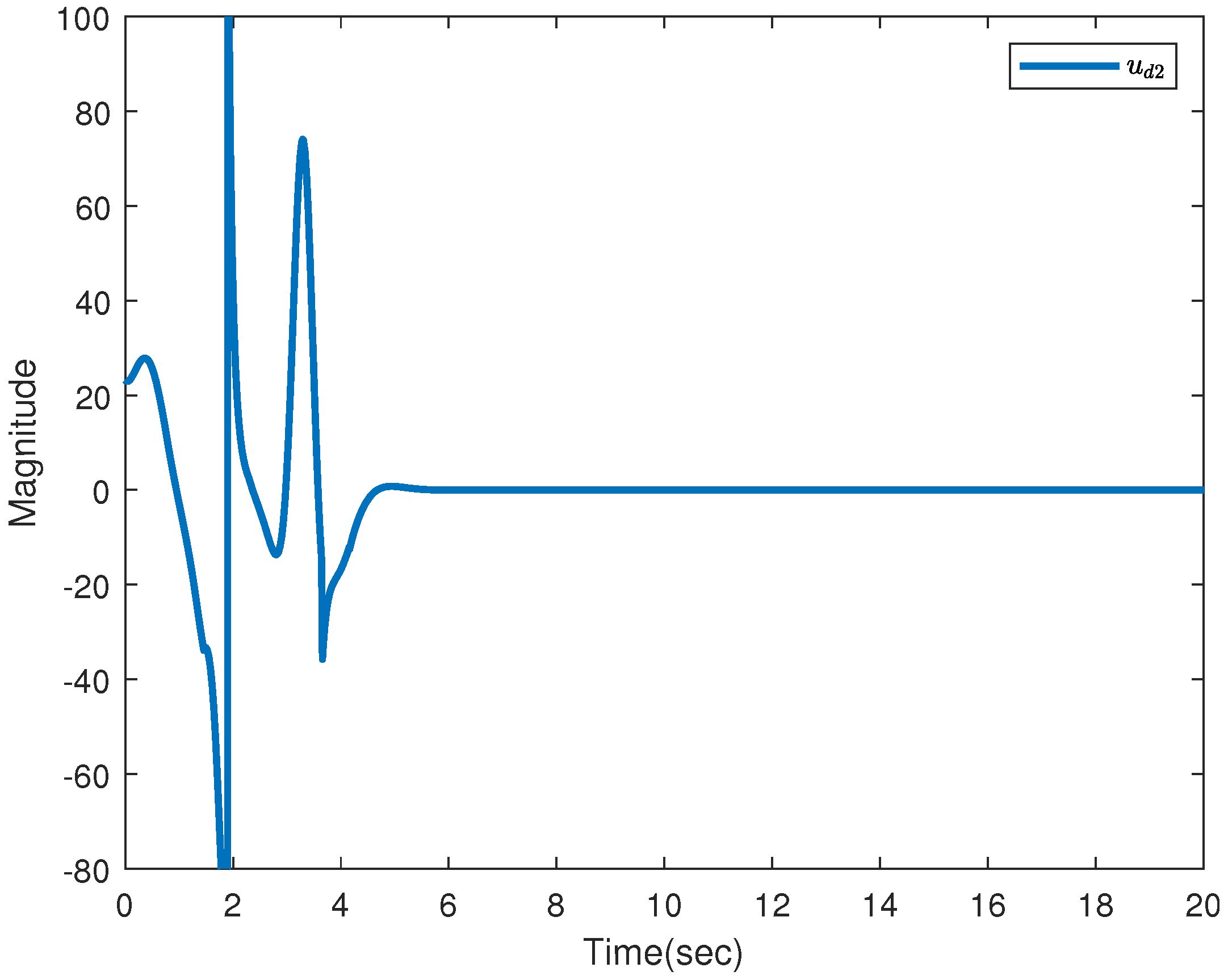
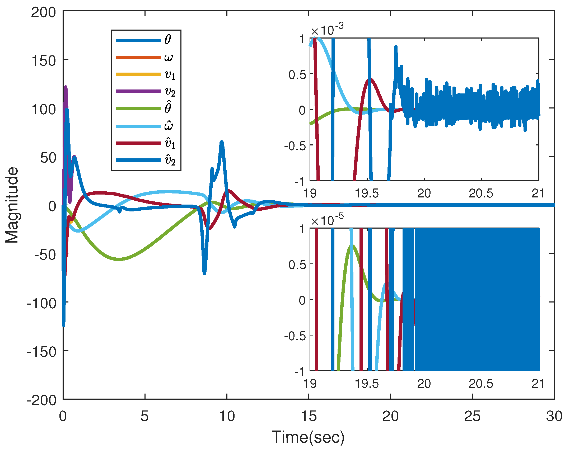
6.2. PMSM Simulations

To verify the performance of the proposed control law (21) and (22) in the presence of deterministic disturbances and stochastic noises, numerical simulations were run for the system (20) in MatLab 2020a, using the values in Section 5.1. The deterministic disturbance was selected as $u_q=0.1t+0.001\cos \left(10t\right)$, and the value of the coefficient $K_5$ was calculated according to the PMSM technical parameters as $K_5=4024.14$. Accordingly, the Lipschitz constant was set to $L=443$. The stochastic noise parameter was given by $r=0.75$. The stochastic convergence was regarded in the mean-square sense, $\rho =2$, to satisfy the conditions of Theorem 3.

It was assumed that only the variable $\theta$ can be measured. Therefore, the observer (16) was used to reconstruct the unmeasured state variables, and the applied control input (21) and (22) was based on the estimates produced by the observer.

Figure 9 shows that the control input (21) and (22), based on the estimates produced by the observer (16), drives all the states of the full-scale 4D PMSM system to the origin within the predefined time of 20 s, again with the precision ${10}^{-4}$, even for high disturbance magnitudes of order ${10}^3$. It can be observed from Figure 10 that the magnitude of the nominal control input $u_{d2}$ still remains acceptable. In this simulation, the control input (21) and (22) is activated after $T=4$ s, when the observer (16) converges according to (18), to avoid unreasonably high control magnitudes. Note that the obtained results still provide better convergence precision and a lesser control magnitude than those presented in [17] for close values of the PMSM parameters and deterministic disturbances, even in the presence of additional stochastic noise.

Finally, Figure 11 displays the compensator control input (22) $v\left(t\right)$, based on the estimates produced by the observer (16), against the disturbance $\xi \left(t\right)=K_5{u}_q=4024.14(0.1t+0.001\cos \left(10t\right))$ in the presence of a white noise with diffusion $v_2^{0.75}$. It can be observed that the control input $v\left(t\right)$ reliably compensates for the disturbance soon after the initial time moment for a stochastic system as well.

7. Conclusions

This paper has presented a predefined-time convergent robust control algorithm that allows the control designer to set the convergence time in advance, independently of initial conditions, deterministic disturbances, and stochastic noises. In contrast to most existing finite- and fixed-time control techniques, a predefined-time convergent control law enables one to explicitly assign the desired convergence time equal to the true one in disturbance-free cases and make it closer to the true one in the presence of deterministic disturbances and/or stochastic noises. The simulation results obtained for a full-scale 4D PMSM system show that the designed control law is capable of driving the PMSM system states to an equilibrium point for a pre-assigned time and operates with control magnitudes suitable for practical applications such as electrical vehicles, trains, industrial robots, unmanned autonomous vehicles, and others. Our ongoing research focuses on further improving the performance of predefined-time convergent control algorithms and designing predefined-time convergent adaptive control laws for multi-dimensional systems with uncertain parameters.

References

- Lu, W.; Liu, X.; Chen, T. A note on finite-time and fixed-time stability. Neural Netw. 2016, 81, 11–15. [Google Scholar] [CrossRef] [Green Version]
- Sánchez-Torres, J.D.; Gómez-Gutiérrez, D.; López, E.; Loukianov, A.G. A class of predefined-time stable dynamical systems. IMA J. Math. Control Inf. 2018, 35, I1–I29. [Google Scholar] [CrossRef] [Green Version]
- Polyakov, A.; Efimov, D.; Perruquetti, W. Finite-time and fixed-time stabilization: Implicit Lyapunov function approach. Automatica 2015, 51, 332–340. [Google Scholar] [CrossRef] [Green Version]
- Polyakov, A. Characterization of finite/fixed-time stability of evolution inclusions. In Proceedings of the 2019 IEEE 58th Conference on Decision and Control (CDC), Nice, France, 11–13 December 2020; pp. 4990–4995. [Google Scholar]
- Matsuoka, K. Development trend of the permanent-magnet synchronous motor for railway traction. IEEJ Trans. Electr. Electron. Eng. 2007, 2, 154–161. [Google Scholar] [CrossRef]
- Zhang, Q.; Liu, X. Permanent magnetic synchronous motor and drives applied on a mid-size hybrid electric car. In Proceedings of the 2008 IEEE Vehicle Power and Propulsion Conference, Harbin, China, 3–5 September 2008; pp. 1–5. [Google Scholar]
- Torrent, M.; Perat, J.I.; Jiménez, J.A. Permanent-magnet synchronous motor with different rotor structures for traction motor in high speed trains. Energies 2018, 11, 1549. [Google Scholar] [CrossRef] [Green Version]
- Staszak, J.; Ludwinek, K.; Gawecki, Z.; Kurkiewicz, J.; Bekier, T.; Jaskiewicz, M. Utilization of permanent-magnet synchronous motors in industrial robots. In Proceedings of the 2015 International Conference on Information and Digital Technologies, Zilina, Slovakia, 7–9 July 2015; pp. 342–347. [Google Scholar]
- Wu, X.; Zhang, B. Sensorless model reference adaptive control of permanent magnet synchronous motor for industrial robots. In Proceedings of the 2019 8th International Symposium on Next Generation Electronics (ISNE), Zhengzhou, China, 9–10 October 2019; pp. 2019–2021. [Google Scholar]
- Suti, A.; Rito, G.D.; Galatolo, R. Fault-tolerant control of a three-phase permanent magnet synchronous motor for lightweight UAV. Actuators 2021, 10, 253. [Google Scholar] [CrossRef]
- Zhao, Y.; Qiao, W.; Wu, L. Sensorless control for IPMSMs based on a multilayer discrete-time sliding-mode observer. In Proceedings of the 2012 IEEE Energy Conversion Congress and Exposition (ECCE), Raleigh, NC, USA, 15–20 September 2012; pp. 1788–1795. [Google Scholar]
- Azzoug, Y.; Sahraoui, M.; Pusca, R.; Ameid, T.; Romary, R.; Cardoso, A.J. A Variable Speed Control of Permanent Magnet Synchronous Motor Without Current Sensors. In Proceedings of the 2020 IEEE 29th International Symposium on Industrial Electronics (ISIE), Delft, The Netherlands, 17–19 June 2020; pp. 1523–1528. [Google Scholar]
- Zhao, Y.; Qiao, W.; Wu, L. Improved Rotor Position and Speed Estimators for Sensorless Control of Interior Permanent-Magnet Synchronous Machines. IEEE J. Emerg. Sel. Top. Power Electron. 2014, 2, 627–639. [Google Scholar] [CrossRef]
- Awan, H.A.A.; Tuovinen, T.; Saarakkala, S.E.; Hinkkanen, M. Discrete-time observer design for sensorless synchronous motor drives. IEEE Trans. Ind. Appl. 2016, 52, 3968–3979. [Google Scholar] [CrossRef]
- Deo, H.V.; Shekokar, R.U. A review of speed control techniques using PMSM. Int. J. Innov. Res. Technol. 2014, 1, 2349–6002. [Google Scholar]
- Ren, Z.; Ma, J.; Qi, Y.; Zhang, D.; Koh, C.S. Managing uncertainties of permanent-magnet synchronous machine by adaptive Kriging assisted weight index Monte-Carlo simulation method. IEEE Trans. Energy Convers. 2020, 35, 2162–2169. [Google Scholar] [CrossRef]
- Basin, M.; Rodriguez-Ramirez, P.; Ramos-Lopez, V. Continuous fixed-time convergent controller for permanent-magnet synchronous motor with unbounded perturbations. J. Frankl. Inst. 2020, 357, 11900–11913. [Google Scholar] [CrossRef]
- Aguilar Mejía, O.; Tapia Olvera, R.; Rivas Cambero, I.; Minor Popocatl, H. Adaptive speed controller for a permanent-magnet synchronous motor. Nov. Sci. 2019, 11, 142–170. [Google Scholar] [CrossRef]
- Van, M.; Mavrovouniotis, M.; Ge, S.S. An adaptive backstepping nonsingular fast terminal sliding mode control for robust fault tolerant control of robot manipulators. IEEE Trans. Syst. Man Cybern. Syst. 2019, 49, 1448–1458. [Google Scholar] [CrossRef] [Green Version]
- Gao, S.; Wei, Y.; Zhang, D.; Qi, H.; Wei, Y. A modified model predictive torque control with parameters robustness improvement for PMSM of electric vehicles. Actuators 2021, 10, 132. [Google Scholar] [CrossRef]
- Lakhe, R.K.; Chaoui, H.; Alzayed, M.; Liu, S. Universal control of permanent magnet synchronous motors with uncertain dynamics. Actuators 2021, 10, 49. [Google Scholar] [CrossRef]
- Van, M.; Ge, S.S.; Ren, H. Finite-time fault tolerant control for robot manipulators using time delay estimation and continuous nonsingular fast terminal sliding mode control. IEEE Trans. Cybern. 2017, 47, 1681–1693. [Google Scholar] [CrossRef]
- Van, M. An enhanced robust fault tolerant control based on an adaptive fuzzy PID-nonsingular fast terminal sliding mode control for uncertain nonlinear systems. IEEE/ASME Trans. Mechatron. 2018, 23, 1362–1371. [Google Scholar] [CrossRef] [Green Version]
- Basin, M. Finite- and fixed-time convergent algorithms: Design and convergence time estimation. Annu. Rev. Control 2019, 48, 209–221. [Google Scholar] [CrossRef]
- Jiménez-Rodríguez, E.; Muñoz-Vázquez, A.J.; Sánchez-Torres, J.D.; Loukianov, A.G. A note on predefined-time stability. IFAC-PapersOnLine 2018, 51, 520–525. [Google Scholar] [CrossRef]
- Lopez-Ramirez, F.; Efimov, D.; Polyakov, A.; Perruquetti, W. On necessary and sufficient conditions for fixed-time stability of continuous autonomous systems. In Proceedings of the 2018 European Control Conference (ECC), Limassol, Cyprus, 12–15 June 2018; pp. 197–200. [Google Scholar]
- Pal, A.K.; Kamal, S.; Nagar, S.K.; Bandyopadhyay, B.; Fridman, L. Design of controllers with arbitrary convergence time. Automatica 2020, 112, 108710. [Google Scholar] [CrossRef]
- Jimenez-Rodriguez, E.; Sanchez-Torres, J.D.; Loukianov, A.G. Backstepping design for the predefined-time stabilization of second-order systems. In Proceedings of the 2019 16th International Conference on Electrical Engineering, Computing Science and Automatic Control (CCE), Mexico City, Mexico, 11–13 September 2019; pp. 1–6. [Google Scholar]
- Garza-Alonso, A.; Basin, M.; Rodriguez-Ramirez, P. Predefined-time stabilization of permanent-magnet synchronous motor. Trans. Inst. Meas. Control 2021, 43, 3044–3054. [Google Scholar] [CrossRef]
- Wang, G.; Zhang, G.; Xu, D. Position Sensorless Control Techniques for Permanent Magnet Synchronous Machine Drives; Springer: Berlin/Heidelberg, Germany, 2020. [Google Scholar]
- Levant, A. Homogeneity approach to high-order sliding mode design. Automatica 2005, 41, 823–830. [Google Scholar] [CrossRef]
- Ménard, T.; Moulay, E.; Perruquetti, W. Fixed-time observer with simple gains for uncertain systems. Automatica 2017, 81, 438–446. [Google Scholar] [CrossRef] [Green Version]