A Novel Deep Learning Model for Mechanical Rotating Parts Fault Diagnosis Based on Optimal Transport and Generative Adversarial Networks

Abstract

To solve the poor real-time performance of the existing fault diagnosis algorithms on transmission system rotating components, this paper proposes a novel high-dimensional OT-Caps (Optimal Transport–Capsule Network) model. Based on the traditional capsule network algorithm, an auxiliary loss is introduced during the offline training process to improve the network architecture. Simultaneously, an optimal transport theory and a generative adversarial network are introduced into the auxiliary loss, which accurately depicts the error distribution of the fault characteristic. The proposed model solves the low real-time performance of the capsule network algorithm due to complex architecture, long calculation time, and oversized hardware resource consumption. Meanwhile, it ensures the high precision, early prediction, and transfer aptitude of fault diagnosis. Finally, the model’s effectiveness is verified by the public data sets and the actual faults data of the transmission system, which provide technical support for the application.

1. Introduction

Mechanical rotating components are the critical components of the transmission system. However, the failure is almost inevitable because of the long-time dynamic running of the components [1,2,3,4]. Once a failure occurs, the entire transmission system will be shut down. Therefore, effective early fault diagnosis of mechanical rotating components will significantly improve the transmission system’s reliability and reduce downtime. A lot of studies have been conducted on early fault diagnosis algorithms for mechanical rotating components [5,6,7,8,9,10]. However, several problems still exist, such as high recognition accuracy but complex algorithm architecture, and simple algorithm logic but low recognition accuracy, which lead to a difficulty for practical application.

Traditional maintenance methods can be divided into two types: repair maintenance and preventive maintenance. Repairable maintenance often refers to repairing equipment after failure. The biggest drawback is that it will affect the production plan. At the same time, the cost of spare parts and labor for emergency repairs will also bring high repair costs to the professional maintenance team. Preventive maintenance planned regular equipment maintenance and replacement of parts and components, usually including maintenance, regular inspections, regular functional testing, regular disassembly and repair, regular replacement, and other methods. Regular maintenance requires the overall assessment and maintenance of equipment shutdown. The disadvantage is that it takes a long time, is low in efficiency, and brings new failure risks.

The two maintenance methods have been gradually outdated in the mature era of IoT and big data, so predictive maintenance has emerged as the times require. This new maintenance method can predict the time of failure and maintain the equipment in real-time and efficiently. However, in the application process of predictive maintenance mode, some practical problems have gradually emerged. Assuming that all the massive data generated daily are collected and uploaded to the cloud for analysis and processing, they will inevitably cause a huge load on the network. It will not be easy to meet the real-time requirements of critical services.

Some new solutions have also emerged in response to the large network load, low real-time requirements, and poor accuracy encountered in traditional predictive maintenance. For example, some early solutions for predictive maintenance algorithms for integrated transmission systems have high fault diagnosis accuracy: Shalalfeh [11] proposed a new method to analyze the multi-dimensional sensory data and used the characteristics of the technique to conduct health prediction. A detrended fluctuation analysis was utilized to evaluate the long-term correlation in the rolling bearing vibration data. The test results showed that Kendall’s tau coefficient could be deemed an early warning signal of bearing failure, but the real-time performance was poor due to the long correlation in the time domain. Jia [12,13] proposed an intelligent diagnosis method based on a neural network. A multi-layer perceptron deep learning network was used to diagnose bearing faults with an accuracy of 99.74%, but the model architecture is very complicated. Ince [14] proposed a fast and accurate early fault diagnosis algorithm to monitor the motor operating status by using an adaptive one-dimensional convolutional neural network. Meanwhile, the feature extraction and the classification stages of motor fault detection were fused into a single learning body. The experimental results verified the effectiveness of the method. However, it cannot be applied in practice due to poor real-time performance. He then proposed a bearing fault diagnosis method based on deep learning [15]. This method used a short-time Fourier transform (STFT) to preprocess the sensor signal. A large memory storage retrieval neural network (LAMSTAR) neural network was established. The experiments showed that the bearing fault could be diagnosed effectively, but the early data-driven model is required to complete the fault diagnosis.

With the rapid development of machine learning, many methods such as a novel model, deep inception net with atrous convolution (ACDIN) [16], convolutional neural network [17,18,19,20], long and short-term memory hybrid neural network [21], and deep belief nets [22], and combined vibration images [23], deep encoder [24] and other deep learning models were applied to the field of fault diagnosis. Moreover, both the data sets and the actual test data were used to verify their effectiveness. However, these methods are computationally expensive and cannot be suitable for real-time applications.

Sabour [25] proposed a deep network with activation vectors based on classic deep learning and convolutional neural networks. The network expanded the ordinary neurons in the deep network into the multi-dimensional neurons and encapsulated the multi-dimensional data into a capsule network. The multi-dimensional neurons can obtain the size and direction information of the data and had stronger learning capabilities compared with the ordinary neuron networks. However, the introduction of the iterative algorithm based on dynamic routing and unsupervised clustering brought extra loop iteration while using the network, resulting in a greater hardware resource consumption and a longer calculation time.

Wang [26] combined the capsule network with the Xception module (XCN) to achieve intelligent fault diagnosis. Firstly, a wavelet time-frequency analysis was performed to obtain the fault time-frequency diagram. Secondly, the XCN was input for training, and the cost function penalty was performed on the parameters, which changed considerably. Finally, the fault types were classified according to the envelope length by the dynamic routing operation. Zhu [27] built a fault recognition network with a depth of 12 layers and a network parameter of 7.9M by combining the inception network with the capsule network. The time-frequency diagram of the vibration signal was obtained by preprocessing to diagnose the fault of the rotating part. Due to a large number of parameters in the network architecture, it is hard to reduce the computation time. Wang [28] proposed an envelope network based on a wide convolution and multi-scale convolution for fault diagnosis. The proposed capsule network based on wide convolution and multi-scale convolution (WMSCCN) algorithm used a one-dimensional vibration signal as the input signal. At the same time, the adaptive batch normalization (AdaBN) algorithm was introduced into the model. The effectiveness of the algorithm is verified through experiments, but the fault recognition accuracy is low. Kao [29] proposed an effective fault diagnosis algorithm. The fault diagnosis is based on the current signature analysis. A complete faulty motor diagnosis system needs to perform feature extraction based on existing methods and then perform additional classification methods. The first is a classification method using wavelet packet transform and a deep one-dimensional convolutional neural network containing a softmax layer. The experimental results using real-time data of motor stator current prove the effectiveness of this method for real-time monitoring of motor status. When this method is training, a high-specification PC may be needed to train a neural network containing a large number of neurons, and the real-time performance is poor. Zhang [30] proposed an enhanced CNN model that uses time-frequency images as input for bearing fault diagnosis. Seven data sets provided by CWRU and YSU are used to verify the effectiveness of the proposed method. The training time of this method is relatively short, and the accuracy rate is as high as 96%, but the model has poor robustness. Zhao [31] proposed an improved DCGAN (deep CNN based GAN) for vibration-based fault diagnosis with unbalanced data. An auxiliary classifier is introduced to facilitate the training process, and an AE-based method is introduced to estimate the similarity of the generated samples. At the same time, an online sample filter is designed and embedded in GAN for automatic sample selection, where the selected samples should meet the requirements of accuracy and diversity. This method has good diagnostic performance, but the time cost of parameter adjustment is too long, and the reliability is low.

In summary, the early fault diagnosis algorithms based on traditional methods have problems such as complex data preprocessing, poor applicability, and low recognition accuracy. Deep learning abstracts and encodes the original features by constructing a multi-layer perceptual structure and then realizes the classification or recognition of samples. The more layers and neurons the deep learning model has, the more features and storage details it can obtain. Deep learning in image processing and natural language processing has achieved outstanding results, but with the development of deep learning model, the depth of each neuron in the network only consists of one feature, its ability to obtain and mine information is limited; because of the expansion of neurons to dimensional vector, each dimension of learning has different features, and it can learn to get more information. Hinton [25,32] proposed two vector structure deep networks, vector CapsuleNet and matrix CapsuleNet. These two networks expand pixels into multidimensional vectors, and the expanded neurons are called Capsules. Capsule replaces a single neuron of the original neural network. For this purpose, the introduction of deep learning algorithms into the early fault diagnosis process of the transmission system can effectively improve the capabilities of early fault diagnosis. Despite CapsuleNet dynamic routing algorithm for high-dimensional vectors and a large number of training samples, the calculation time is much longer than other deep learning networks of the same scale. The algorithm has high complexity, a large calculation amount, a long calculation time, and high hardware requirements. Due to this limitation, the routing algorithm cannot be applied to the real-time processing of vibration signals of mechanical rotating parts in the integrated transmission system of actual vehicles. In the case of high real-time requirements and limited equipment terminal computing capabilities, the existing complex deep learning network architecture needs to be improved in order to propose a deep network algorithm with simple architecture, small amount of calculation, high real-time performance, and robust data mining capabilities to realize early real-time fault diagnosis of rotating components.

It contains two pieces of information: the magnitude of the vector and the direction of the vector. It uses an iterative update method to transmit the Capsule information between the two layers dynamically. CapsuleNet has two main contributions to the deep network: one is to expand the dimension of neurons and enhance the ability of the network to obtain information; the other is that the transmission of the two-layer Capsule adopts dynamic routing algorithm and Expectation–Maximization algorithm to realize non-features supervised cluster learning.

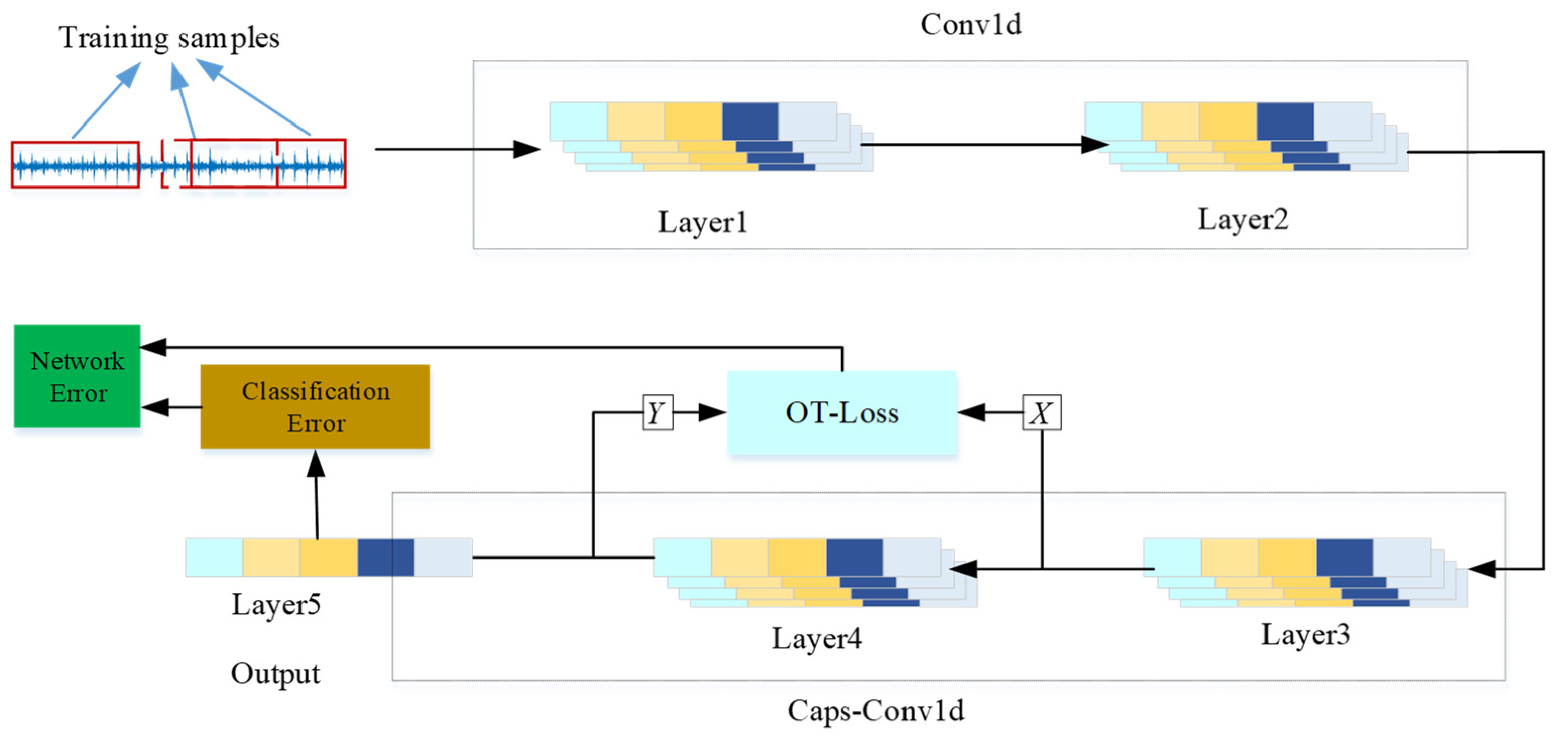
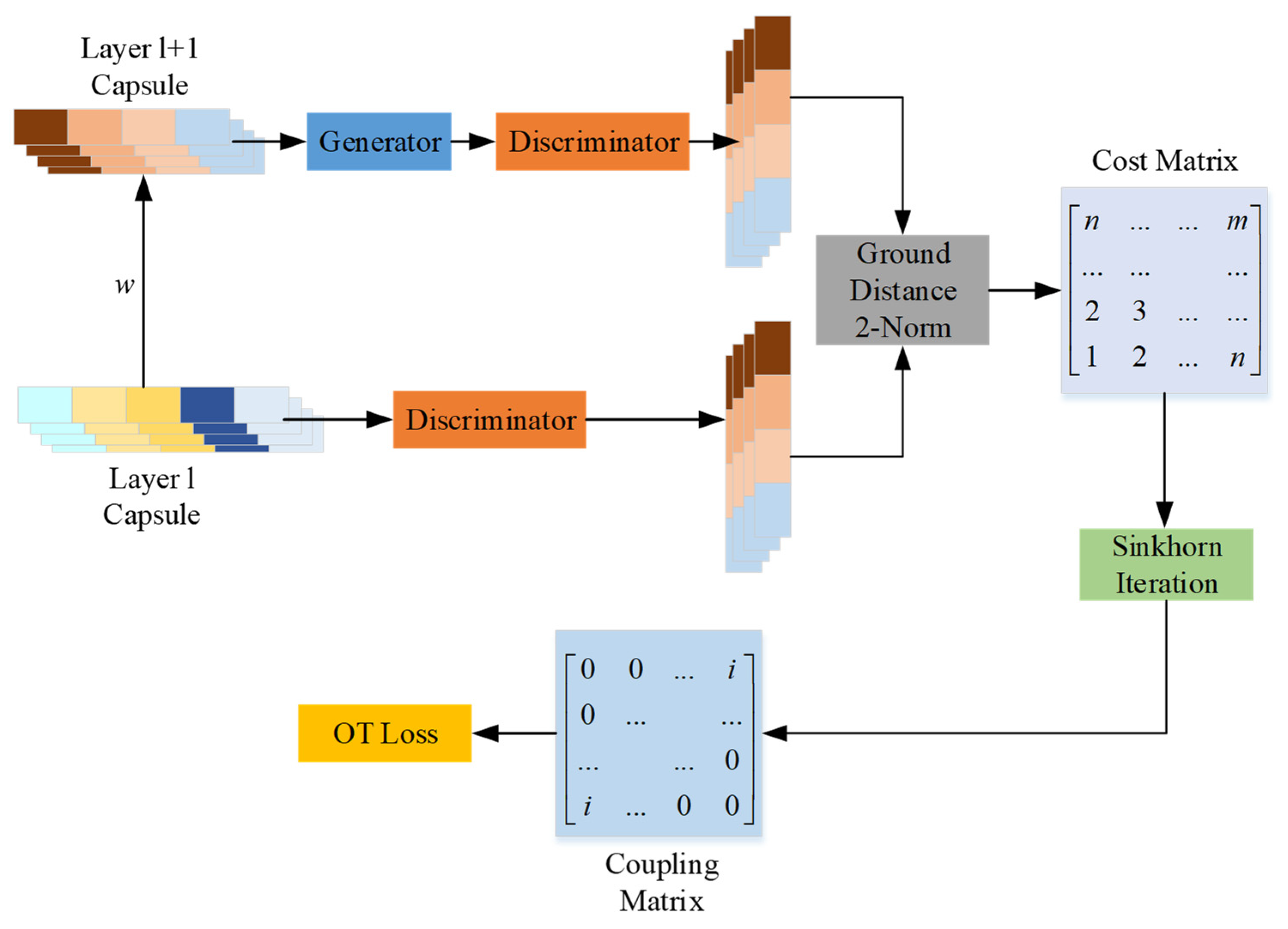
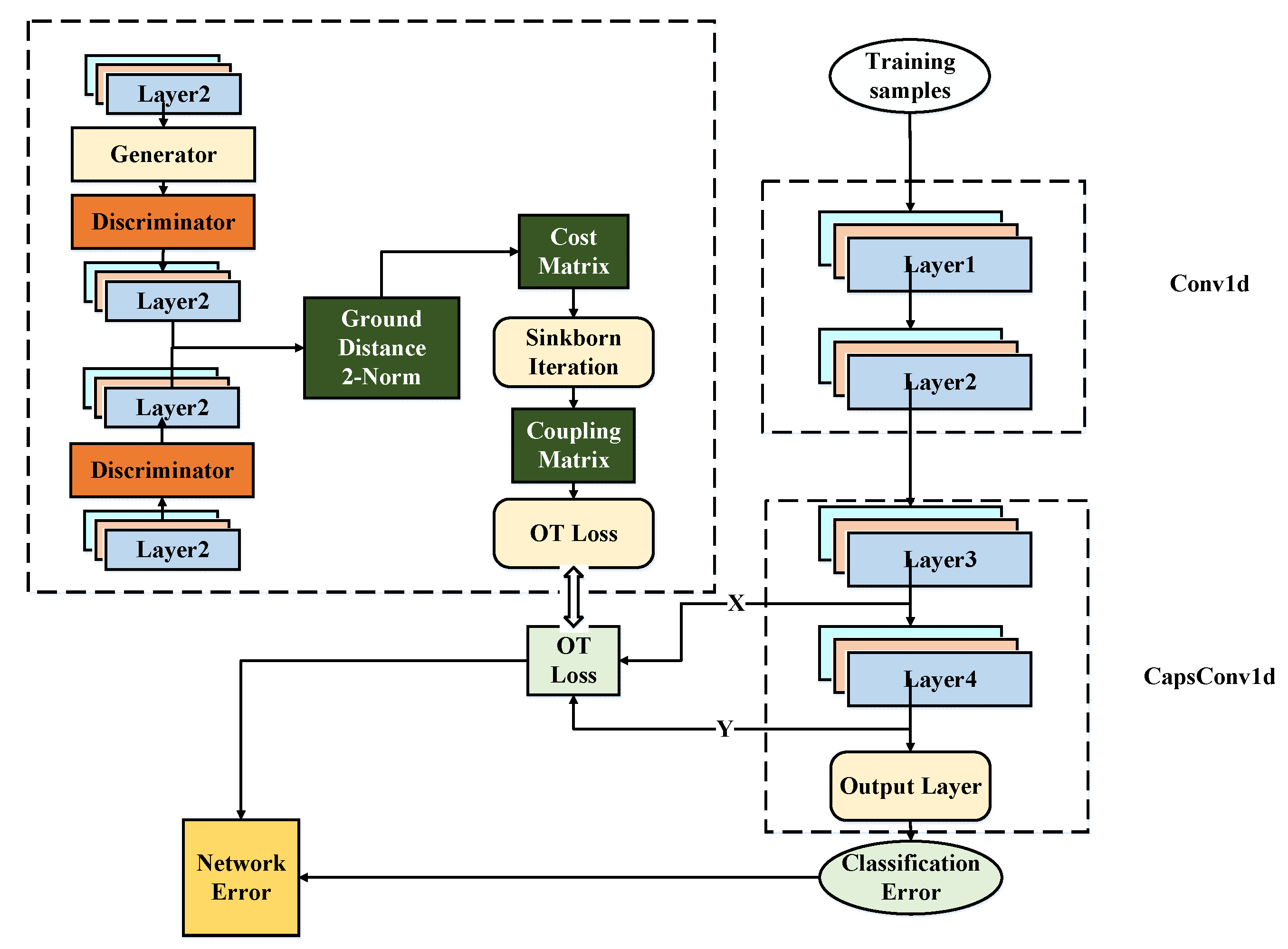
Due to the high complexity, a large amount of calculation, and the long time consuming of the capsule network algorithm [25], in order to implement the actual vehicle deployment, the routing update algorithm needs to be improved to solve the iterative update process, reduce the amount of calculation, and improve the real-time performance of the calculation. This paper uses optimal transport and generative adversarial networks to replace the routing update algorithm and further modifies the capsule network architecture to realize the processing of one-dimensional original vibration data. This paper proposes the OT-Caps fault diagnosis model, which has more robust fault feature mining capabilities and better recognition accuracy. It solves the problems of poor real-time performance, large calculation volume, and high hardware platform requirements of the capsule network and provides a basis for actual deployment applications.

The main contribution of this paper is to propose a novel fault diagnosis model named OT-Caps. Based on the capsule network’s characteristics, the model expands the one-dimensional neuron in the traditional convolutional neural network into the multi-dimensional neuron, which enhances the deep network data mining ability and fault feature storage ability. High-precision identification of multiple failure modes in rotating parts such as bearings, gears, and shafts can be accomplished by collecting raw vibration signals. Simultaneously, the model introduces the generative adversarial networks and the optimal transport theory to construct the objective loss function, which solves the problem of large calculation volume and long calculation time for the multi-dimensional neuron network. The fault identification transferability, fault identification ability, and real-time computing ability of the model are verified by the public data sets and actual vibration data.

The second chapter mainly introduces the proposed OT-Caps algorithm architecture based on the generative adversarial networks and the optimal transport theory. The third chapter mainly introduces the test results of the OT-Caps algorithm under different test data sets and actual test data. The fourth chapter mainly introduces the conclusion.

2. The Proposed Fault Diagnosis Method

2.1. OT-Caps Model Architecture

To realize the online recognition of the abnormal state of the transmission system, the OT-Caps model is designed in this paper, from where the designed network architecture is shown in Figure 1. The OT-Caps fault diagnosis network’s input samples are one-dimensional raw data, and each sample contains 2048 data points. Layer1 and Layer2 are standard rectified linear unit (ReLU) convolutional layers, which perform the vibration data’s preliminary processing. Layer3, Layer4, and Layer5 are capsule convolutional layers, in which convolution, normalization, maximum pooling, and other processes are all operated on the entire capsule. During the training process, the GAN network is used to calculate the error between the input and output features of the capsule convolutional layer, and the optimal transport theory is utilized to calculate the error OT (optimal transport) loss. The OT loss of all layers is then added to the object loss function. Since the object loss function includes both the fault recognition error and the sample distribution error, the network parameter training can be optimized from two aspects. Since there is no need to calculate the OT loss, the network calculation burden gets reduced significantly. The OT-Caps fault diagnosis model proposed in this research mainly improves the traditional capsule network in two aspects as follows:

(1)

The network architecture has been improved to enable the capsule network to directly process the one-dimensional original vibration signal, from where the complexity of data processing is reduced;

(2)

The Generative Adversarial Networks (GAN) and optimal transport theory replace the original routing iteration algorithm to calculate the characteristic distribution error. Compared with the traditional model, the complexity and the calculation time are reduced, and the real-time performance of fault diagnosis is improved.

Layer1 and Layer2 are convolutional networks of ReLU that include expansion layer, convolution layer, pooling layer, normalization layer, and activation layer. Among them, the filling layer expands the data boundary to avoid the influence of the convolution operation on the data length. The filling layers of Layer1 and Layer2 are 28 and 1, respectively. The convolution process is shown in Equation 1. During the feature extraction, the large-size convolution kernel is used to extract the contour features, and the small-size convolution kernel is used to extract the fine features. Since the fault data fluctuate greatly due to noise, the large-size convolution kernel is used to achieve the filtering. The size of the large convolution kernel in Layer1 is set to 64, and the step size of the convolution kernel is 8. Considering that the small convolution kernel can extract fine features, convolution kernel size and the convolution kernel step size of Layer2 are both set to 1. In this structure, the first layer is used to perform filtering algorithm processing on the original signal, and the second layer is used to extract the detailed features of the signal. The input of Layer1 is set to 1 channel, the output is 16 channels, and the output of Layer2 is 32 channels. Setting multiple channels can effectively improve the ability to extract fault features.

$$out\left(C_{ot{t}_j}\right)=bias\left(C_{\mathrm{outf}}\right)+{\displaystyle \sum _{k=0}^{C_{in}-1}\mathrm{kernel}}\left(C_{{\mathrm{out}}_j},k\right)\otimes input(k)$$

(1)

where C is the channel number, k is the size of the convolution kernel and $\otimes$ is the cross-correlation operator.

The pooling process is mainly used to perform the down-sample of the signal. A suitable pooling step size is helpful to enhance the generalization ability as well as improve the transferability of the model. Layer1 and Layer2 use the maximum pooling operation, the pooling step is 2, and the data length after the pooling operation is reduced to half of the original one. In the capsule layer, the maximum pooling operation with a step length of 2 is also adopted, and the pooling process is mainly performed on the capsule unit.

The normalization layer is used to solve the problems of gradient disappearance and gradient explosion during the training process. In addition, the normalization process can make all data distributed in the same scale range, which solves the problem of different fault data scales and improves the ability to recognize and process data characteristics. The normalization process is:

Input: an aggregate S contains x, $S=x_1,x_2,\dots ,x_m$; and parameters γ, β.

Output:

$$\left\{y_i=B{N}_{\gamma ,\beta }(x_i)\right\}$$

(2)

$$\mu \leftarrow \frac{1}{m}{\displaystyle \sum _{i=1}^m{x}_i}$$

(3)

$${\widehat{x}}_i\leftarrow \frac{x_i-\mu }{\sqrt{{\sigma }^2+\epsilon }}$$

(4)

$$y_i\leftarrow \gamma {\widehat{x}}_i+\beta \equiv B{N}_{\gamma ,\beta }(x_i)$$

(5)

The above Equations (2)–(5) are the calculation process of normalization operation and zoom operation respectively, and γ and β are the parameters that the neural network needs to train.

The activation layer introduces a nonlinear operation step into the neural network, which is mainly used to improve the feature extraction ability of the network. Commonly used activation functions mainly include Sigmoid, tanh, ReLU, etc. Among them, the ReLU activation function can achieve a faster convergence rate than Sigmoid and tanh in the process of stochastic gradient descent and has lower computational complexity. Therefore, the ReLU activation function is used as the activation function in the Layer1 and Layer2 of the ordinary convolutional network, as shown in Equation (6).

$$\mathrm{Re}\mathrm{LU}(x)=\max (0,x)$$

(6)

In the original capsule network, the capsule dimension is fixed due to the limitation of the routing update algorithm. Therefore, the OT-Caps fault diagnosis model proposed in this article uses GAN network and optimal transport theory to construct a routing transmission algorithm, which is more flexible than the original network architecture, and the capsule dimension can be flexibly expanded or reduced. The capability of fault feature extraction is much stronger.

The detailed parameters of the OT-Caps network are shown in

Table 1. Detailed parameters of OT-Caps network.

Number	Layer	Convolution Kernel/Step Size/Channel	Number of Parameters	Output Dimension
1	Conv1	64/8/16	1072	(16,128)
2	Conv2	1/1/32	608	(32,65)
3	Caps1	-	768	(32,4,8)
4	Caps2	-	3840	(32,8,1)
5	output	-	2560	(10,8)

. The network takes one-dimensional raw vibration data with a length of 2048 as the input data. Layers 1 and 2 are the ordinary neural network convolutional layers, and Layers 3 and 4 are the capsule layers. Since there is no convolution kernel in the ordinary sense, the capsule layer convolution kernel, step size, and the number of channels is not listed in Table 1. The input data of Layer3 are one-dimensional, which is expanded to 4-dimensional after the dimensional expansion. After Layer4, the output feature is increased to 8 dimensions. All capsules in the Layer3 and Layer4 are 32 channels, that is, the length of each capsule is 32. The last layer is the fully connected layer, from where the output of the layer has the same number of failure modes, that is, the number of the capsules represents the number of the failure modes.

In the training process, the number of the auxiliary error parameters of the OT-Caps network is 121,555. Since the auxiliary error network parameters need to be removed during the training process, the final number of network parameters is 10,384. The detailed parameters are shown in Table 1. The number of capsule network parameters proposed by Zhu [27] is 7.9M, which is 760 times of the network parameters in this paper. Since this network has been optimized and adjusted in terms of network architecture simplification, it can be seen that the adoption of a heterogeneous network effectively reduces the number of network parameters.

2.1.1. OT-Caps Network Objective Loss Function

In order to ensure that the fault data obtained during the fault diagnosis process of the OT-Caps network contain both the fault mode information and sample distribution information, the objective function consists of two parts, which are the error loss caused by the fault pattern recognition error and the error caused by the difference in the capsule distribution between the two layers of the network. The two parts of the error are calculated by the boundary loss and OT loss, respectively.

The length of the capsule module is used to indicate the probability that fault categories the output feature belongs to, and the length and the probability are positively correlated. The calculation of the error caused by the fault pattern recognition of the boundary loss is shown in Equation (7):

$$L_k=T_k\max {\left(0,m^{+}-\Vert v_k\Vert \right)}^2+\lambda \left(1-T_k\right)\max {\left(0,\Vert v_k\Vert -m^{-}\right)}^2$$

(7)

where k represents the type of failure mode. The input sample belongs to the k-th failure mode, and T_k can only be 0 or 1. m⁺ is the upper bound, which punishes the false positives, that is, false samples are mistaken as true; m⁻ is the lower bound, which punishes the false negatives, that is, positive samples are mistaken as true. λ is the proportional coefficient, which is used to adjust the proportion of the two bounds. The total loss is the sum of the losses of all samples. Here m⁺ = 0.9, m⁻ = 0.1, λ = 0.5. In addition, if k exists, $\Vert v_k\Vert$ will not be less than 0.9. If k does not exist, $\Vert v_k\Vert$ will not be greater than 0.1. The importance of penalizing false positives is twice of penalizing false negatives.

OT loss is obtained through the optimal transmission theory and the generative adversarial networks, and the result is

$$OTloss={\displaystyle {\sum }_M{\overline{w}}_Q^M}$$

(8)

which represents the optimal transport loss of the M-layers network structure. The loss function of the OT-Caps model is the combination of the two losses above, as shown in Equation (9):

$$E=L_{mxgin}(t,v)+\beta {\displaystyle \sum _M{\overline{w}}_Q^M}$$

(9)

2.1.2. OT-Caps Network Training Optimization Algorithm

Here t and v are the real category and the predicted category of the input features respectively, and β is the weight coefficient of the OT loss.

After obtaining the object loss function, the OT-Caps network is trained using the samples with the marked failure modes. Because the Adam optimization algorithm combines the advantages of momentum and RMSProp (root mean square prop) optimization algorithms; it has the advantages of fast convergence and strong anti-noise ability. Thus, the Adam (Adaptive Moment Estimation) optimization algorithm is selected here to train the model. The specific steps are shown as follows:

(1)

Input learning rate: the parameters include the attenuation coefficient for moment estimation ${\rho }_1$, ${\rho }_2$, the constant term $\sigma$, the initialize neural network coefficients $\delta$, the initialize first and second moment variables $s=0$, $r=0$, and the number of iterations $t=1$;

(2)

Use the training set data to train the model and output the loss value e;

(3)

Calculate the gradient and update the number of iterations:

$$g\leftarrow {\nabla }_{\theta }L\left(f_{\theta }(x),y\right)t\leftarrow t+1;$$

(4)

Update the first moment variable:

$$s\leftarrow {\rho }_{1}s+\left(1-{\rho }_1\right)g;$$

(5)

Update the second moment variable:

$$r\leftarrow {\rho }_{2}r+\left(1-{\rho }_2\right)g\odot g;$$

(6)

Correct the deviation of the first and second moments:

$$\widehat{s}\leftarrow \frac{s}{1-{\rho }_1^t},\widehat{r}\leftarrow \frac{r}{1-{\rho }_2^t};$$

(7)

Calculation update factor value:

$$\mathsf{\Delta }\theta =-LR\frac{\widehat{s}}{\sqrt{\widehat{r}}+\delta };$$

(8)

Update factor: $\theta \leftarrow \theta +\mathsf{\Delta }\theta$, repeat steps 2 to 8.

2.2. OT-Caps Network Feature Distribution Error Acquisition Algorithm

The routing and transmission algorithm of the OT-Caps model is shown in Figure 2. The l + 1 layer capsule generates features with the same dimension as the l layer through the GAN network generator. The features then input into the discriminator network together with the original l layer output features to obtain two characteristic spatial distribution characteristics. The grounding distance between any two capsules in the feature set is obtained through the Euclidean distance matrix to form a cost matrix. Then the coupling matrix is obtained by Sinkhorn iteration, and the distribution error between the feature sets is obtained. Finally, the distribution error is added into the network objective loss function to train and optimize the network parameters.

2.2.1. GAN Network Computing Feature Distribution

GAN is an improvement to unsupervised learning. It is a new unsupervised architecture. GAN includes two independent networks, which serve as targets for adversarial. The first set of networks is the discriminator we need to train to distinguish whether it is real data or fake data; the second set of networks is a generator that generates random samples similar to real samples and uses them as fake samples. Using the GAN network generator to train the automatic generator and the discriminative can calculate the error of the input and output features of the CapsuleNet convolutional layer. After training, the classification error can be effectively reduced. The distribution error is added to the network objective loss function to train the network parameters. In addition, the GAN network and the optimal transmission theory are used to calculate the characteristic distribution error, replacing the high-complexity routing iterative algorithm, thereby reducing the complexity of the algorithm, reducing the calculation time, and improving the real-time performance of fault diagnosis.

Suppose the characteristic of the capsule of the layer l is $X_l$, the characteristic of the latter layer is $X_{l+1}$, the input capsule unit of the layer l is $\left\{X_l\right\}$, and the output of the layer l capsule is $\left\{X_{l+1}\right\}$. The distribution of $\left\{X_l\right\}$ and $\left\{X_{l+1}\right\}$ after the encoding process are consistent. The GAN network generator is used to reconstruct the capsule of the latter layer, and the generated network only plays a role in restoring the $\left\{X_{l+1}\right\}$ dimension, without changing its distribution characteristics. Therefore, $\left\{X_{l+1}\right\}$ can obtain the same characteristics as the dimension $\left\{X_l\right\}$ after passing through the generator. The generator uses a single-layer network $g_{\theta }$, where $\theta$ represents the generator network parameters. The generator network operation is shown in Equation (10):

$$X_l^{recon}=g_{\theta }(X_{l+1})$$

(10)

A two-layer deep network $f_{\phi }$ is used to instead the discriminator, which is used to calculate the spatial distribution of sample $\left\{X_l\right\}$ and $X_l^{recon}$. $\phi$ represents the parameters of the discriminator network, as shown in Equation (11):

$$P_r=f_{\phi }(X_l),P_g=f_{\phi }(X_l^{recon})$$

(11)

where $P_r$ and $P_g$ represent the distribution of two samples after passing through the discriminant network $f_{\phi }$. By calculating the divergence between the two distributions, the error of the two distributions can be obtained. Then this error is added to the objective function in the network. In the training process of back propagation, all the network parameters are trained to keep the feature distribution consistent. In the fault diagnosis, the GAN is no longer used in the network to simplify the network architecture. This reduces the amount of calculation and improves the calculation efficiency significantly.

2.2.2. Measurement of Data Distribution Error

After obtaining the distribution of the l layer and the l + 1 layer through the discriminator, the divergence of the two distributions needs to be calculated. WD (Wasserstein distance) [33] is a distribution measure obtained by the optimal transmission theory. The optimal transmission theory studies the problem of transformation between distributions. It was first proposed by the French mathematician Monge in the 1780s. The existence of the solution was proved by the Russian mathematician Kantorovich. The French mathematician Brenier established the optimal transmission problem and the internal connection between convex functions. With the extraction of the approximate solution method of the optimal transmission problem, it plays an increasingly important role in the field of mathematics and machine learning today.

WD is defined as

$$W\left(P_r,P_g\right)=\underset{\gamma \in \Pi \left(P_r,P_g\right)}{\inf }{E}_{x,y~y}c(x,y)$$

(12)

Among them, $P_r$ is the feature distribution of the $l$ layer, $P_g$ is the feature distribution of the $l+1$ layer, ${\displaystyle \prod \left(P_r,P_g\right)}$ is the joint distribution probability density between any two points of $p$ and $g$, expressed as $\gamma (x,y)$, and $p(x)$ is the distribution of $p$ and $g$, respectively. The marginal distribution probability,$g(y)$, is the distribution probability of $r$ and $g$ own samples, and $c(x,y)$ is the loss size.

It satisfies the positive definiteness and symmetry, and satisfies the triangular inequality, which is an accurate measure of the geometric distribution of features. WD has many advantages over other distances and divergences. When the unknown parameter $\theta$ is continuous, the loss function is also continuous and basically differentiable everywhere. This provides conditions for parameter modification through the gradient descent method. Compared with other distances and divergence, WD Divergence is more sensitive to the spatial distribution of data, and differences in distribution will cause significant changes, while other distances and divergences do not meet this condition. WD considers the spatial distribution characteristic information, and the convergence of WD is equivalent to the weak convergence of the distribution. Based on the above advantages, this paper chooses the WD measure of the two distributions.

In order to describe the proposed method more intuitively, we have added a flowchart as shown in Figure 3.

3. Experiment Method

In order to verify the effect of the OT-Caps model on fault diagnosis designed in this paper, data sets such as gearbox fault data, bearing failure data, and actual test fault data of the transmission system are used to conduct the verification.

The computer used in this article is configured with an Intel Core (TM) i7-6700 CPU, SDRAM is 16G, the graphics card is NVIDIA GTX 980, and video memory is 4G. We are using GPU-based pytorch1.0 for model training and testing.

3.1. OT-Caps Fault Diagnosis Algorithm Real-Time Comparison Verification

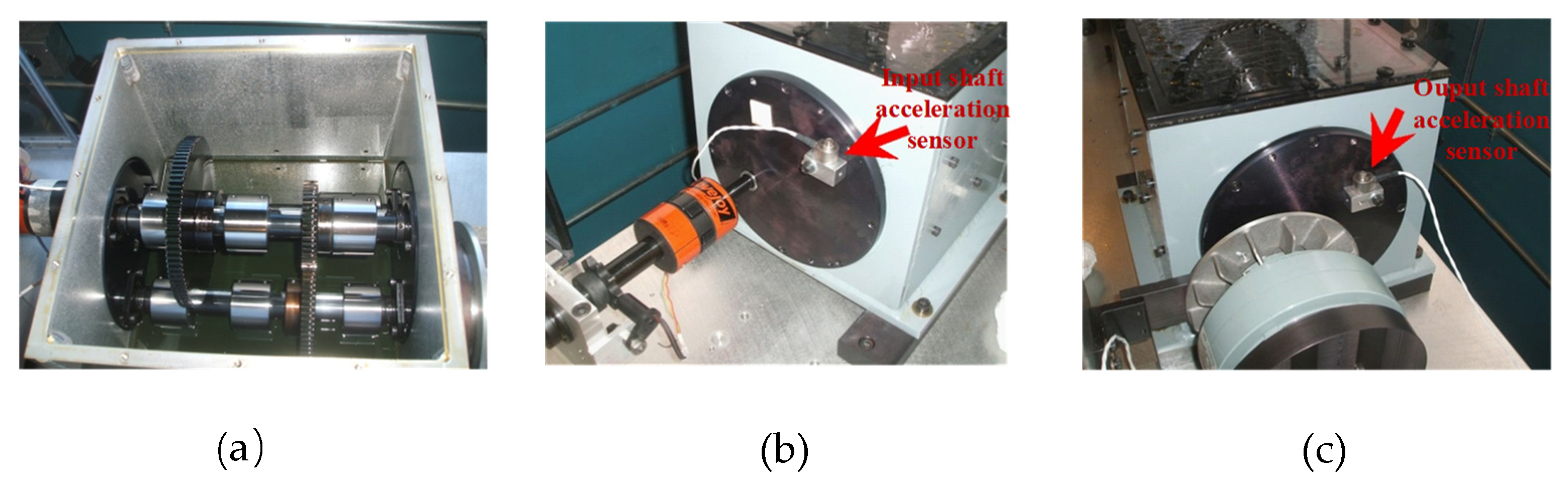
The gearbox failure data in this test are selected from IEEE PHM (Prognostics Health Management) 2009. The structure of the test gearbox is shown in Figure 4a. The input shaft is equipped with gear, the intermediate shaft is equipped with two gears, and the output shaft is equipped with gear. The shaft and the box are connected by bearings, and vibration sensors are respectively installed at the input shaft end and the output shaft end. The number of teeth of the above-mentioned gears is 32, 96, 48, and 80, respectively. The input speed during the test is 30, 35, 40, 45, and 50rpm. The load is divided into high load and low load. The data sampling rate is 66.7kHz. The endurance of each sampling is 4s, and one sample has approximately 256,000 data points. The installation position of the vibration sensor is shown in Figure 4b,c, which is used to collect vibration signals at the input and output ends, respectively.

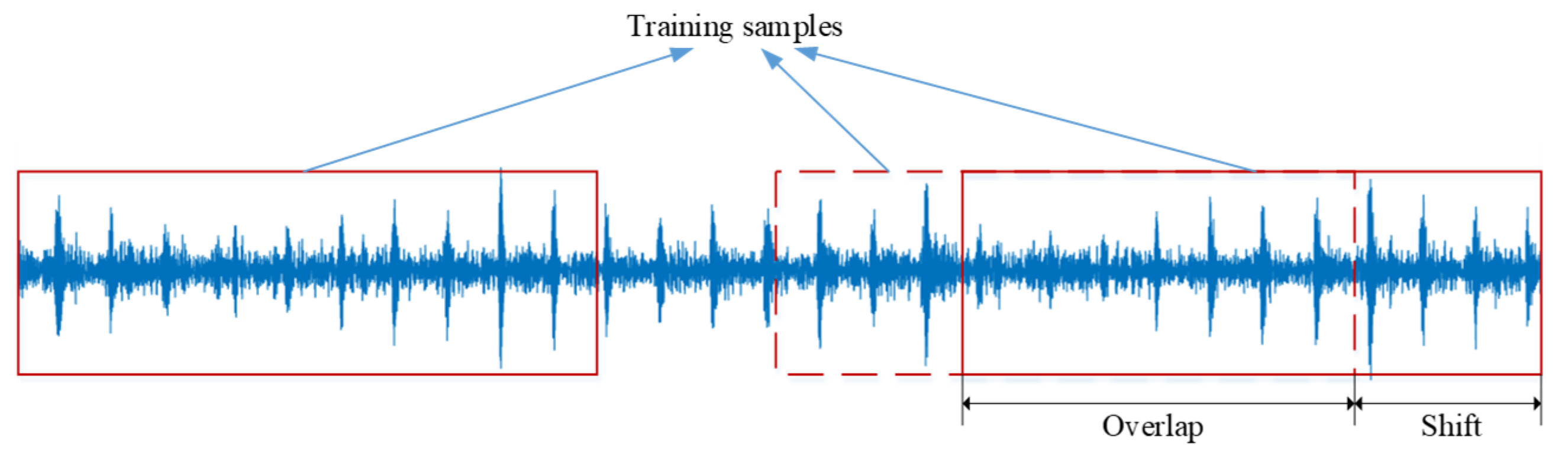
Since the OT-Caps model performs the fault diagnoses on one-dimensional time series vibration signals, from where the fault features can be extracted directly from the original data, the frequency domain analysis is not required. In order to increase the amount and diversity of the training data, this paper uses the sliding window method to perform repeated slice processing on one-dimensional collected data, as shown in Figure 5. The sliding window length is 2048, and the sliding step length is 100. Thus 2048 data points are taken every 100 points. The number of generated samples is 8500, of which 7000 samples are used for training, and 1500 samples are used for testing.

3.1.1. OT-Caps Network Training Optimization Algorithm

In this part, the OT-Caps fault diagnosis model was compared with the original CapsuleNet model in terms of training time, test running time, and recognition accuracy. The original CapsuleNet can be found in [25], from which the input is a two-dimensional vector. Here, the original vibration data is directly converted into a two-dimensional vector to meet the input requirements of CapsuleNet. The comparison results of the two network models are shown in

Table 2. Comparison results with the CapsuleNet.

Network Type	Training Sample	Time/s	Test Samples	Time/s	Test Accuracy
CapsuleNet	7500	331.25	1000	17	84.78%
OT-Caps	7500	24.43	1000	0.13	99.45%

. It can be found from the table that the calculation time of the improved OT-Caps model in this paper is much lower. During the training process, the training speed of the OT-Caps model is 13.5 times that of the original CapsuleNet model. During the test, because the OT-Caps fault diagnosis model uses the OT loss solution process, its operation speed is 130 times that of CapsuleNet, which shows a great advantage. According to the time-consuming test, its data processing rate is 7.692kHz, which has the ability to meet the real-time requirements for fault diagnosis of mechanical rotating parts of the transmission system.

3.1.2. Comparison of Fault Recognition Accuracy

The test accuracy of various deep fault diagnosis models was then compared, and the diagnosis results are shown in

Table 3. Comparison of gearbox fault diagnosis accuracy.

Network Type	DTS-CNN	1-DCNN	DACNN	OT-Caps
Diagnosis accuracy	99.37%	99.34%	99.3%	99.45%

. Among the tested models, the dislocated time series CNN (DTS-CNN) can be found in Reference [34], the one-dimensional convolutional neural network (1-DCNN) can be found in Reference [35], and the deep adversarial convolutional neural network (DACNN) can be found in Reference [36]. Through comparison, it can be seen that the OT-Caps proposed in this paper also has good recognition accuracy.

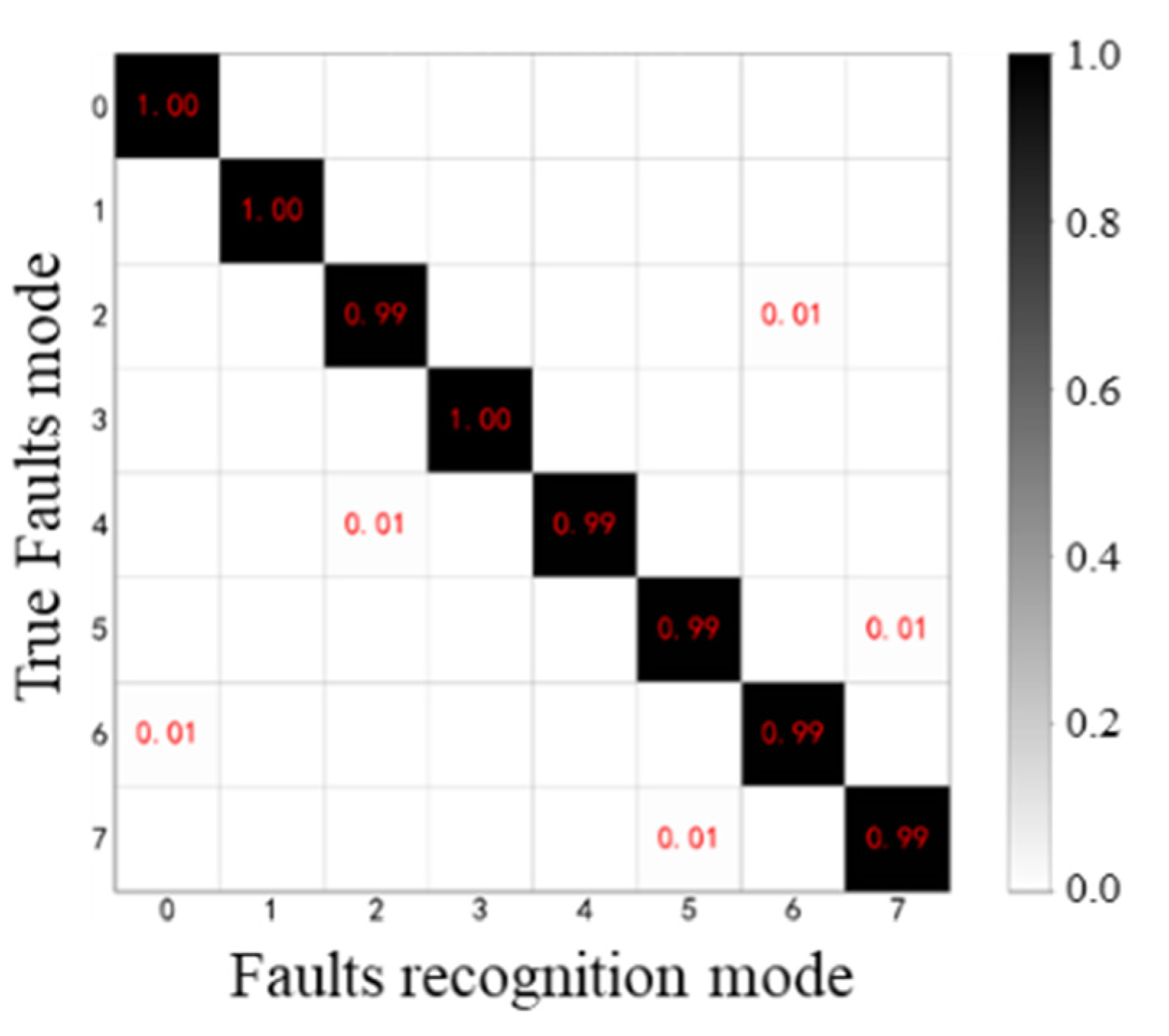
The fault recognition confusion matrix is used to identify the probability of recognition errors between the failure modes. Figure 5 shows the gearbox fault recognition confusion matrix. Figure 6 and Table 3 show that the OT-Caps fault diagnosis model has high recognition accuracy for eight types of faults.

3.2. OT-Caps Transfer Capability Comparison Verification

The bearing failure test data set used in this paper is a set of open standard bearing data from the Data Center of Western Reserve University. Due to its openness and representativeness, many scholars worldwide have carried out related research on this data set such as fault characteristic signal extraction and fault pattern recognition. Different scholars have worked on the same data, which makes the dataset helpful to perform the comparison of fault recognition capabilities of different algorithms.

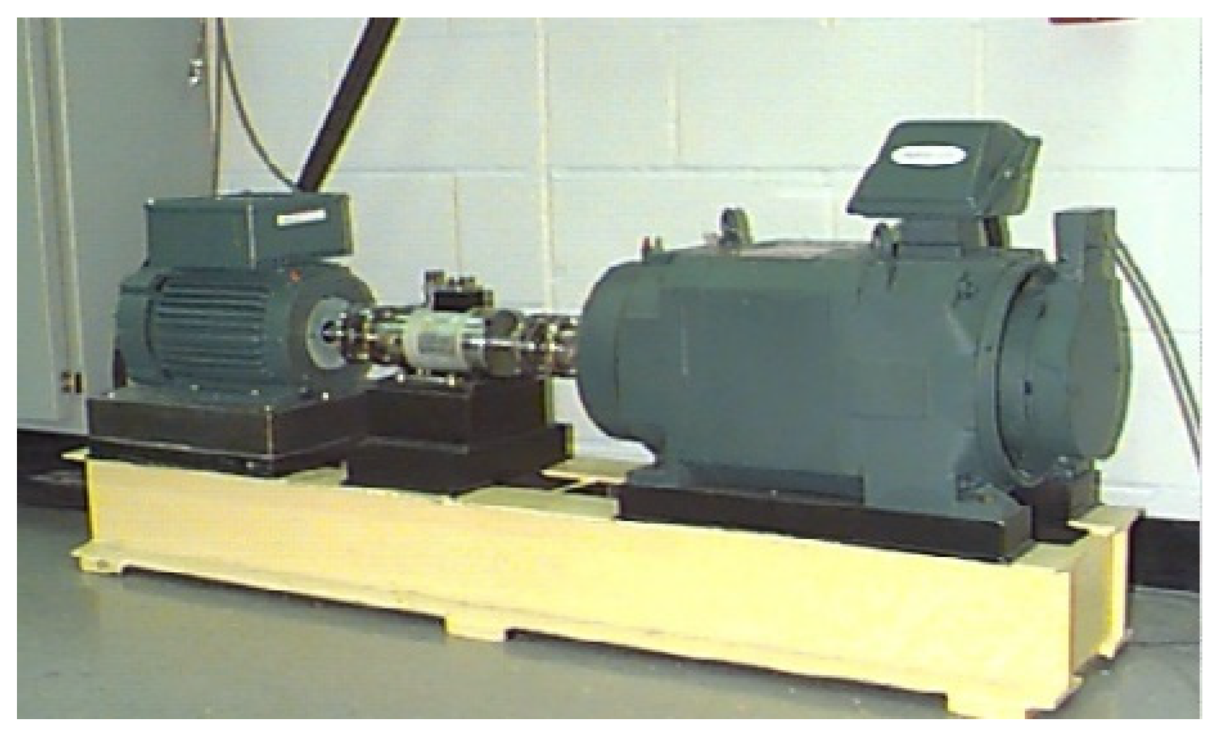
The bearing failure test equipment of Western Reserve University is shown in Figure 7 [27]. The test bench is composed of two motors. The bearing is installed in the bearing box, and the bearing can work under different working conditions by adjusting the different speeds of the motor. The data sets under different working conditions are classified according to the working status.

During the test, all the bearing faults were manufactured manually, and the rolling element, inner ring and outer ring were processed by the electric spark fault injection method. Several sizes of the bearing were used to simulate different fault levels. The test bearing load contained three types, 1, 2, and 3 hp, and the speeds were 1772, 1750, and 1730 rpm, respectively. The failure modes are different under different loads and speeds, including nine different failure modes. Therefore, this data set contained ten working states (including health states) in total.

3.2.1. Data Preprocessing

The vibration data analyzed in this article were collected at the drive end. The sampling frequency was 12 kHz, the sampling time was 10s, and each data set contains 120,000 data points. In order to increase the number of samples, the sliding window length is set as 2048, the sliding step length is 100, and 2048 data points are taken every 100 points, which can generate a total of 6000 samples. Five thousand samples are used for training, and 1000 samples are used for testing. As shown in

Table 4. Bearing working conditions.

Rotating Speed/rpm	Load/hp	Damage Size/Inch	Dataset Name
1772	1	7\14\21	A
1750	2	7\14\21	B
1730	3	7\14\21	C

, according to the different speeds and load, there are three working conditions, which constitute data sets A, B, and C, respectively. One data set is used for training, and the other two data sets are used for testing to verify the fault identification transferability of this model.

3.2.2. Comparison of Experimental Results

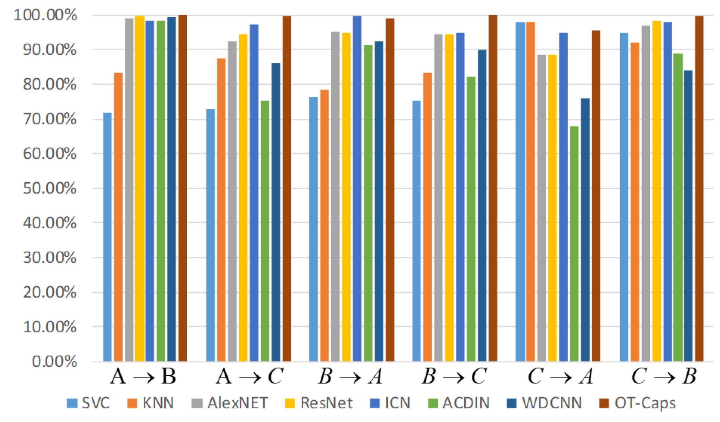
Several algorithms are used to conduct the comparison in this paper, including support vector machine (SVM), k-nearest neighbor (kNN), Support Vector Classification (SVC), and classic architectures such as AlexNet, ResNet, the bearing diagnosis architecture ACDIN mentioned in [16], a deep architecture for bearing fault diagnosis wide first layer kernels (WDCNN) proposed in [37]. Among them, SVC and KNN use frequency spectrum as the input features. AlexNet, ResNet, and Information centric networking (ICN) use time domain spectrogram as the input features. ACDIN, WDCNN, and OT-Caps use raw data as the input features. The fault recognition accuracy of each algorithm is shown in Figure 8 and

Table 5. Comparison of failure mode recognition accuracy.

Algorithm	A→B	A→C	B→A	B→C	C→A	C→B	Mean
SVC	71.93	72.90	76.33	75.30	98.03	94.77	81.55
KNN	83.27	87.33	78.57	83.17	97.80	91.97	87.02
AlexNET	98.93	92.27	95.07	94.40	88.40	96.87	94.32
ResNet	99.70	94.40	94.87	94.33	88.70	98.47	94.58
ICN	98.23	97.17	99.80	94.71	94.93	98.10	97.15
ACDIN	98.30	75.33	91.20	82.30	68.00	88.80	83.99
WDCNN	99.50	86.20	92.40	89.80	76.03	83.90	87.97
OT-Caps	100.00	99.89	99.10	100.0	95.38	99.63	99.00

. According to Figure 8 and Table 5, it can be seen that the prediction accuracy of the deep learning architecture is significantly higher than the two shallow architectures SVC and KNN, indicating that the deep learning architecture can better extract fault features. In the deep learning architecture, the prediction accuracy of the methods which use time domain or frequency spectrum as the input feature is generally higher than the methods that use the original feature as the input feature, indicating that it is more difficult for the deep model to extract features directly from the original data. Because the OT-Caps architecture proposed in this paper can extract the original data features well, and the prediction accuracy is higher than that of other deep models, it shows that OT-Caps has a stronger feature extraction ability.

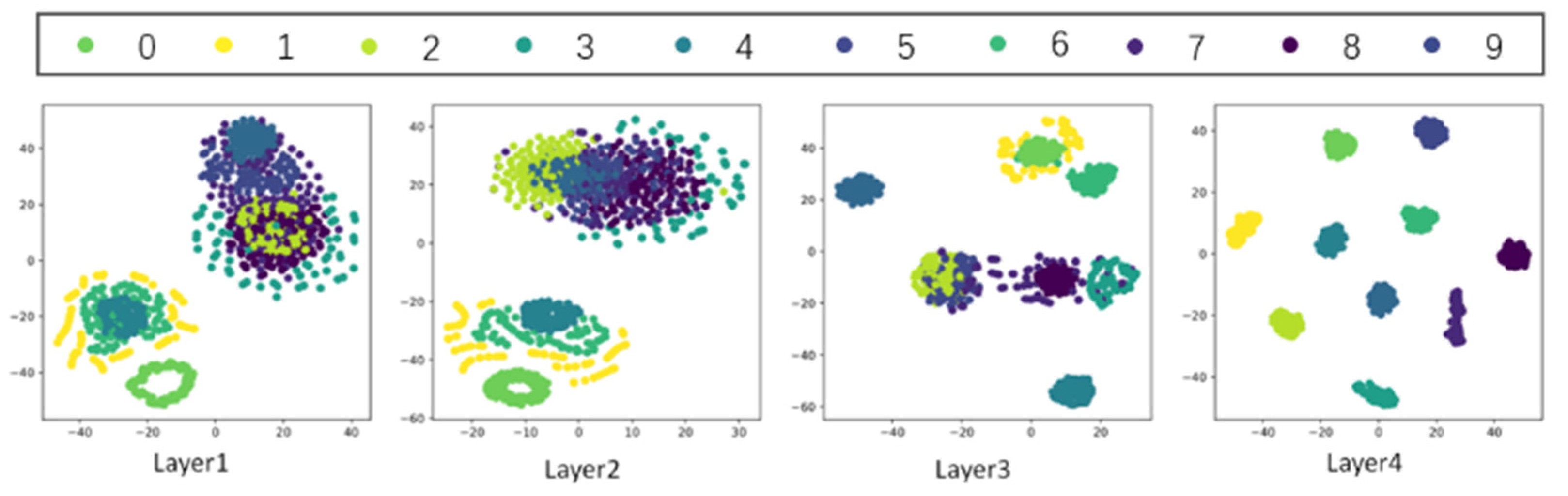
After using t-SNE (t-distributed stochastic neighbor embedding) to cluster the output features of each layer, from where the result can be found in Figure 9, it can be seen that more layers have the better ability to extracted features. Among them, Layer1 and Layer2 are ordinary convolutional networks, and their feature extraction degree is relatively shallow. Layer3 is the capsule layer. After passing through the capsule network, the features have a better degree of discrimination, but certain types of features are still mixed together. Layer4 is the second capsule layer. After the second capsule layer, the features can be distinguished well, and then the learned features are output through the fully connected layer.

3.3. Gearbox Failure Test

In order to verify the effectiveness of the OT-Caps fault diagnosis algorithm for the fault diagnosis of the transmission system, a real failure test was carried out on the gearbox in the transmission system, and the early fault diagnosis ability of the OT-Caps algorithm was verified through the gearbox test data.

3.3.1. Test Equipment

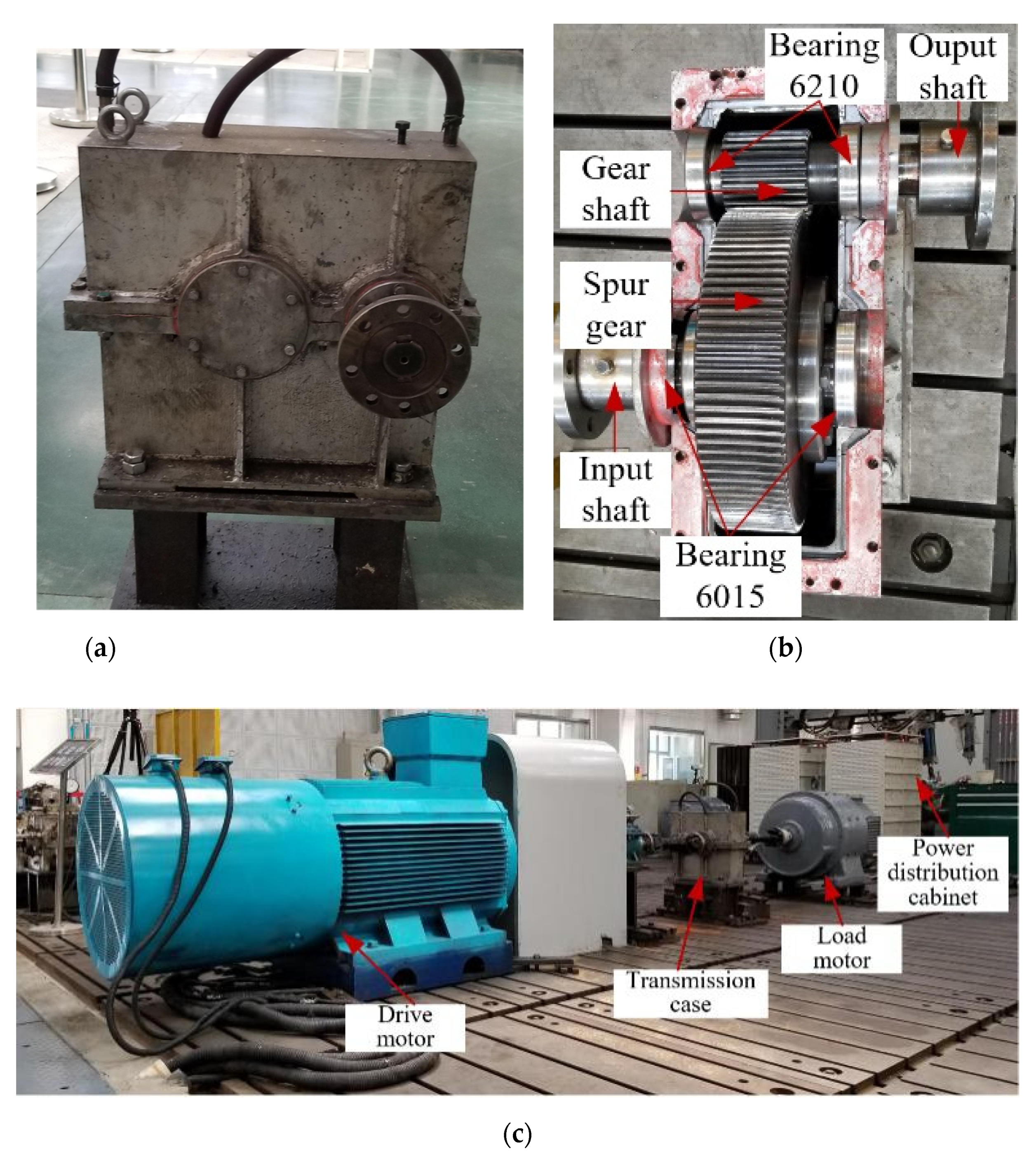
During the test, a spur gear transmission box with a transmission ratio of 1:4 was used as the test object. The test transmission box is shown in Figure 10, including a pair of meshing spur gears and two fixed shafts. Support bearings are installed at both ends of the shaft. The two bearing sizes are 6015 and 6210, respectively. The test process was mainly conducted on the support bearing.

3.3.2. Test Result

Sufficient bearing lubrication is a common failure mode. This testing process mainly simulates the failure of insufficient lubricating oil and is conducted on the transmission system by applying torque loads of different magnitudes at different speeds. During the test, the speed includes 400, 800, 1200 rpm, and the load is 50, 150 and 200 N.m. In order to avoid the gluing of the gearbox bearings which could damage the motor, the test should be stopped immediately when the gearbox vibrates severely. During the experiments, two failure tests were carried out. In the first test, the original bearing in the transmission box was damaged during operation. After replacing the new bearing, the second failure test was then carried out. The test stopped when the strong vibration occurred, and the bearing was damaged again. The test data was captured during the two tests.

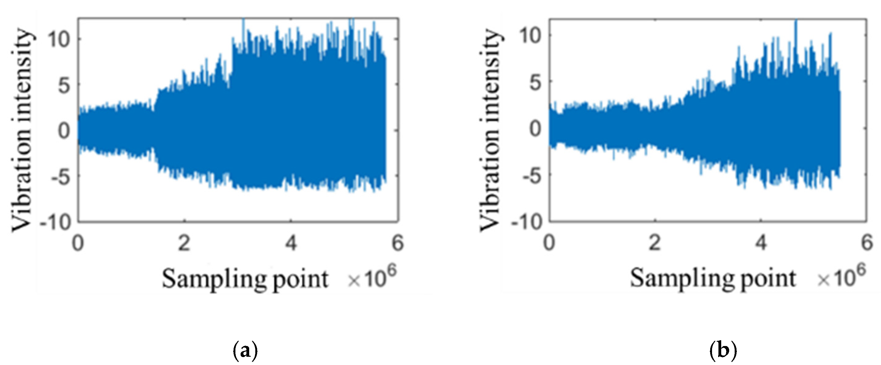
The data sampling rate is 25.6 kHz, and each data set includes about 2560 points. The first bearing runs for 3.12 h and the second bearing runs for 2.97 h. The original data in the Y direction are shown in Figure 11. With the degradation process, the vibration gradually increases. Figure 11a shows the degradation process of the original bearing of the transmission box. The degradation process is not stable because the box has been running for a long time. Figure 11b is the vibration curve of the bearing degradation process in a new state, and the vibration increases significantly with the wear that exists.

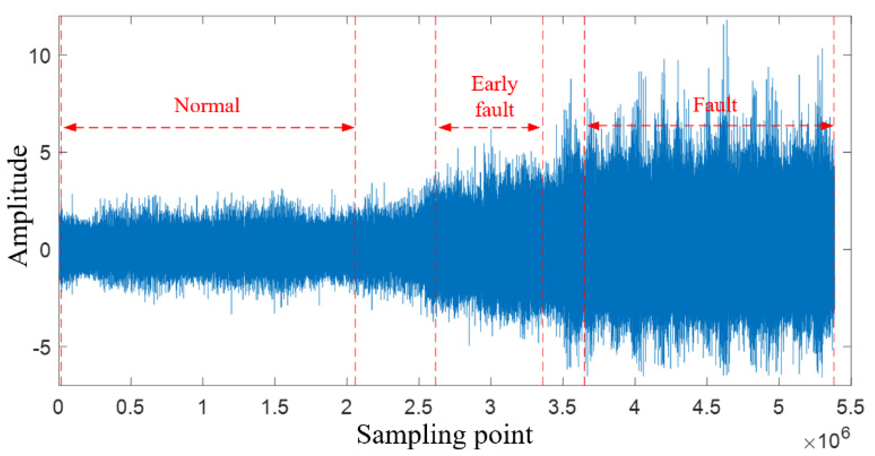
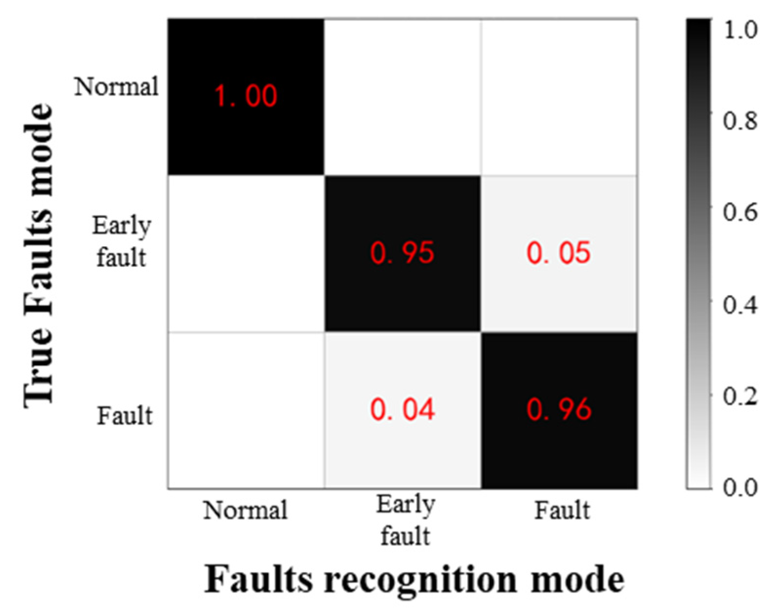
This test data are used to verify the ability of OT-Caps to identify early faults. Early fault identification is mainly based on the increase of the vibration signal and the appearance of periodic shock vibration when the transmission system fails. The vibration data of the transmission box failure process are shown in Figure 12. The red dotted line is the division of the transmission box failure state, which is divided into three stages, which are normal, early failure, and failure stage, according to the degradation process. Taking a certain interval between the two states to avoid the similarity of the samples in the adjacent places of the data results in low sample discrimination. The data preprocessing is the same as the method used before. A total of 3000 samples, composed of three groups and each group containing 1000 samples for a certain state, are generated. Two thousand four hundred samples are randomly selected for training samples, and the other 600 samples are used for testing.

After testing, the fault recognition accuracy of the OT-Caps model is 97.17%, which can effectively identify different damage levels. The fault recognition confusion matrix is shown in Figure 13. There is no recognition error between the normal state and the early fault or fault state. The test results indicate that when the transmission box fails, OT-Caps has the ability to identify early failures effectively.

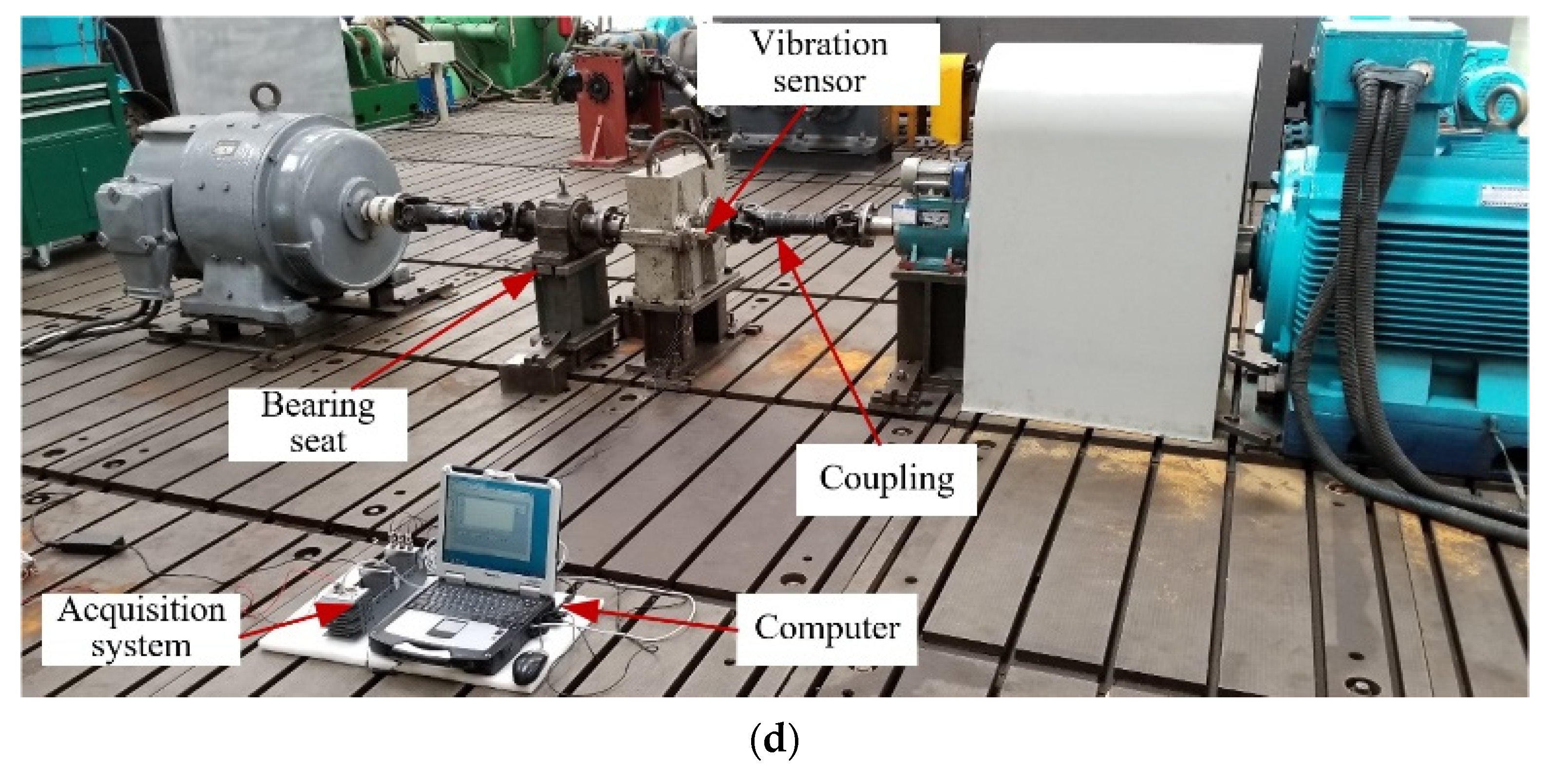
3.4. Bench Test Verification of Integrated Transmission System

3.4.1. Test Equipment

The fault data come from two integrated transmission systems of a certain model undergoing maintenance. Perform a bench test on two units. Install a vibration sensor on the input shaft and output shafts on both sides, and install three vibration sensors on the upper-end cover of the integrated transmission system close to the fan drive link. A total of 6 three-directional acceleration vibration sensors are installed. The Simens LMS acquisition instrument acquires vibration signals.

In the test process, the comprehensive transmission box was mounted in reverse gears 1 and 2, neutral gear, and forward gears 1 to 6, and each gear was carried out for four-speed inputs of 800, 1200, 1600, and 2200rpm. The load is divided into no-load and medium-speed. For three load conditions of low load and full load, the sampling rate is 10 kHz, and each operating condition works for about 5 min.

3.4.2. Test Result

After testing, the classification accuracy of the OT-Caps fault diagnosis model on the test set can reach 100%. The algorithm can effectively identify different failure modes of mechanical rotating parts of the integrated transmission system. The operational efficiency and accuracy of CapsuleNet and OT-Caps are compared. As shown in

Table 6. Comparison results with the CapsuleNet network.

Network Type	Training Sample	Time/s	Test Samples	Time/s	Test Accuracy
CapsuleNet	3500	148.38	850	33.09	99.85%
OT-Caps	3500	11.71	850	0.17	100%

, it can be seen that this network has great advantages in real-time. The CapsuleNet architecture provided by Li [38] is used here, and the network parameter is 10.58M. The OT-Caps fault diagnosis network proposed in this paper, under the premise of achieving high-precision fault diagnosis by reducing the network architecture, reducing network parameters, and improving the network architecture, effectively improves the real-time performance of the fault diagnosis process. It provides technical support for actual vehicle deployment.

4. Conclusions

In this paper, a deep learning algorithm is used to identify the abnormal state of transmission system failure mode. Considering the embedded online usability of deep learning algorithm, a high real-time deep learning algorithm based on the OT-Caps network is proposed. Based on the robust data processing of the CapsuleNet, the network architecture and parameter training algorithm are improved. A simplified high-dimensional neuron network architecture that directly processes the original vibration signal is obtained with a heterogeneous training process and use process network. By introducing an auxiliary error network in the offline training process of the model, the OT-Caps algorithm can solve the problem of low real-time performance caused by complex architecture, long calculation time, and large hardware resource consumption. At the same time, the generative adversarial networks and the optimal transport theory are introduced into the auxiliary error network to accurately describe the fault characteristic distribution error. While improving the real-time performance of the algorithm, it also ensures the high precision, early predictability and transfer of fault diagnosis. Finally, the algorithm’s effectiveness is verified through the public data set and the comprehensive transmission platform failure data, which provides technical support for real vehicle applications.

Although the lightweight OT-caps network can achieve high efficiency and low energy consumption for online deployment, it is still necessary to continue to track the actual vehicle collection data of the integrated transmission system and establish the full life data of the transmission system. At present, the deployed test system has not yet experienced the failure of the mechanical rotating parts of the integrated transmission system. Continue to follow the car to complete the accumulation of the failure data and fatigue degradation data of the mechanical rotating parts of the integrated transmission system. After completing the data, we can deploy and test the PHM system of the integrated transmission system in actual vehicles. In the actual vehicle state, we can realize the comprehensive transmission system failure prediction, do the health management, and realize the transformation from “post-incident maintenance” and “regular maintenance” to “preventive maintenance”.

References

1. Liu, X.; Song, P.; Yang, C.; Hao, C.; Peng, W. Prognostics and Health Management of Bearings Based on Logarithmic Linear Recursive Least-Squares and Recursive Maximum Likelihood Estimation. IEEE Trans. Ind. Electron. 2018, 65, 1549–1558. [Google Scholar] [CrossRef]
2. Lei, Y.; Li, N.; Gontarz, S.; Lin, J.; Radkowski, S.; Dybala, J. A Model-Based Method for Remaining Useful Life Prediction of Machinery. IEEE Trans. Reliab. 2016, 65, 1314–1326. [Google Scholar] [CrossRef]
3. Miao, X.; Li, S.; Zhu, Y.; An, Z. A Novel Real-Time Fault Diagnosis Method for Planetary Gearbox Using Transferable Hidden Layer. IEEE Sens. J. 2020, 20, 8403–8412. [Google Scholar] [CrossRef]
4. Yan, R.; Shen, F.; Sun, C.; Chen, X. Knowledge Transfer for Rotary Machine Fault Diagnosis. IEEE Trans. Reliab. 2020, 20, 8374–8393. [Google Scholar] [CrossRef]
5. Li, X.; Zhang, X.; Li, C.; Zhang, L. Rolling element bearing fault detection using support vector machine with improved ant colony optimization. Measurement 2013, 46, 2726–2734. [Google Scholar] [CrossRef]
6. Li, J.; Huang, R.; He, G.; Wang, S.; Li, G.; Li, W. A Deep Adversarial Transfer Learning Network for Machinery Emerging Fault Detection. IEEE Sens. J. 2020, 20, 8413–8422. [Google Scholar] [CrossRef]
7. Chen, L.; Wang, Z.; Qin, W.; Ma, J. Fault diagnosis of rotary machinery components using a stacked denoising autoencoder-based health state identification. Signal Process. 2017, 30, 377–388. [Google Scholar]
8. Qian, G.; Lu, S.; Pan, D.; Tang, H.; Liu, Y.; Wang, Q. Edge Computing: A Promising Framework for Real-Time Fault Diagnosis and Dynamic Control of Rotating Machines Using Multi-Sensor Data. IEEE Sens. J. 2019, 19, 4211–4220. [Google Scholar] [CrossRef]
9. Soualhi, A.; Medjaher, K.; Zerhouni, N. Bearing Health Monitoring Based on Hilbert–Huang Transform, Support Vector Machine, and Regression. IEEE Trans. Instrum. Meas. 2015, 64, 52–62. [Google Scholar] [CrossRef] [Green Version]
10. Li, N.; Lei, Y.; Lin, J.; Ding, S. An Improved Exponential Model for Predicting Remaining Useful Life of Rolling Element Bearings. IEEE Trans. Ind. Electron. 2015, 62, 7762–7773. [Google Scholar] [CrossRef]
11. Shalalfeh, L.; AlShalalfeh, A.A. Early Warning Signals for Bearing Failure Using Detrended Fluctuation Analysis. Appl. Sci. 2020, 10, 8489. [Google Scholar] [CrossRef]
12. Feng, J.; Lei, Y.; Jing, L.; Xin, Z.; Na, L. Deep neural networks: A promising tool for fault characteristic mining and intelligent diagnosis of rotating machinery with massive data. Mech. Syst. Signal Process. 2016, 72, 303–315. [Google Scholar]
13. Jia, F.; Lei, Y.; Guo, L.; Lin, J.; Xing, S. A neural network constructed by deep learning technique and its application to intelligent fault diagnosis of machines. Neurocomputing 2018, 272, 619–628. [Google Scholar] [CrossRef]
14. Ince, T.; Kiranyaz, S.; Eren, L.; Askar, M.; Gabbouj, M. Real-Time Motor Fault Detection by 1-D Convolutional Neural Networks. IEEE Trans. Ind. Electron. 2016, 63, 7067–7075. [Google Scholar] [CrossRef]
15. He, M.; He, D. Deep Learning Based Approach for Bearing Fault Diagnosis. IEEE Trans. Ind. Appl. 2017, 53, 3057–3065. [Google Scholar] [CrossRef]
16. Chen, Y.; Peng, G.; Xie, C.; Zhang, W.; Li, C.; Liu, S. ACDIN: Bridging the gap between artificial and real bearing damages for bearing fault diagnosis. Neurocomputing 2018, 294, 61–71. [Google Scholar] [CrossRef]
17. Wei, Z.; Li, C.; Peng, G.; Chen, Y.; Zhang, Z. A deep convolutional neural network with new training methods for bearing fault diagnosis under noisy environment and different working load. Mech. Syst. Signal Process. 2018, 100, 439–453. [Google Scholar]
18. Yang, H.; Zhao, F.; Jiang, G.; Sun, Z.; Mei, X. A Novel Deep Learning Approach for Machinery Prognostics Based on Time Windows. Appl. Sci. 2019, 9, 4813. [Google Scholar] [CrossRef] [Green Version]
19. Jiang, G.; He, H.; Yan, J.; Xie, P. Multiscale Convolutional Neural Networks for Fault Diagnosis of Wind Turbine Gearbox. IEEE Trans. Ind. Electron. 2019, 66, 3196–3207. [Google Scholar] [CrossRef]
20. Li, X.; Ding, Q.; Sun, J. Remaining useful life estimation in prognostics using deep convolution neural networks. Reliab. Eng. Syst. Saf. 2018, 172, 1–11. [Google Scholar] [CrossRef] [Green Version]
21. Kong, Z.; Cui, Y.; Xia, Z.; Lv, H. Convolution and Long Short-Term Memory Hybrid Deep Neural Networks for Remaining Useful Life Prognostics. Appl. Sci. 2019, 9, 4156. [Google Scholar] [CrossRef] [Green Version]
22. Shen, C.; Xie, J.; Wang, D.; Jiang, X.; Shi, J.; Zhu, Z. Improved hierarchical adaptive deep belief network for bearing fault diagnosis. Appl. Sci. 2019, 9, 3374. [Google Scholar] [CrossRef] [Green Version]
23. Hoang, D.; Kang, H. Rolling element bearing fault diagnosis using convolutional neural network and vibration image. Cogn. Syst. Res. 2018, 53, 42–50. [Google Scholar] [CrossRef]
24. Shao, H.; Jiang, H.; Lin, Y.; Li, X. A novel method for intelligent fault diagnosis of rolling bearings using ensemble deep auto-encoders. Mech. Syst. Signal Process. 2018, 102, 278–297. [Google Scholar] [CrossRef]
25. Sabour, S.; Frosst, N.; Hinton, G. Dynamic routing between capsules. In Proceedings of the 31st Conference on Neural Information Processing Systems, Long Beach, CA, USA, 4–9 December 2017; pp. 3859–3869. [Google Scholar]
26. Wang, Z.; Zheng, L.; Du, W.; Cai, W.; Zhou, J.; Wang, J.; Han, X.; He, G. A novel method for intelligent fault diagnosis of bearing based on capsule neural network. Complexity 2019, 2019, 1–17. [Google Scholar] [CrossRef] [Green Version]
27. Zhu, Z.; Peng, G.; Chen, Y.; Gao, H. A convolutional neural network based on a capsule network with strong generalization for bearing fault diagnosis. Neurocomputing 2019, 323, 62–75. [Google Scholar] [CrossRef]
28. Wang, Y.; Ning, D.; Feng, S. A Novel Capsule Network Based on Wide Convolution and Multi-Scale Convolution for Fault Diagnosis. Appl. Sci. 2020, 10, 3659. [Google Scholar] [CrossRef]
29. Kao, I.H.; Wang, W.J.; Lai, Y.H.; Perng, J.W. Analysis of permanent magnet synchronous motor fault diagnosis based on learning. IEEE Trans. Instrum. Meas. 2019, 68, 310–324. [Google Scholar] [CrossRef]
30. Zhang, Y.; Xing, K.; Bai, R.; Sun, D.; Meng, Z. An enhanced convolutional neural network for bearing fault diagnosis based on time-frequency image. Measurement 2020, 157, 107667. [Google Scholar] [CrossRef]
31. Zhao, B.; Yuan, Q. Improved generative adversarial network for vibration-based fault diagnosis with imbalanced data. Measurement 2021, 169, 108522. [Google Scholar] [CrossRef]
32. Hinton, G.; Sabour, S.; Frosst, N. Matrix capsules with EM routing. In Proceedings of the 6th international conference on learning representations, ICLR, Vancouver, BC, Canada, 30 April–3 May 2018; pp. 1–15. [Google Scholar]
33. Irpino, A.; Verde, R. Dynamic clustering of interval data using a Wasserstein-based distance. Pattern Recognit. Lett. 2008, 29, 1648–1658. [Google Scholar] [CrossRef]
34. Han, T.; Liu, C.; Yang, W.; Jiang, D. Learning transferable features in deep convolutional neural networks for diagnosing unseen machine conditions. ISA Trans. 2019, 93, 341–353. [Google Scholar] [CrossRef] [PubMed]
35. Wu, C.; Jiang, P.; Ding, C.; Feng, F.; Chen, T. Intelligent fault diagnosis of rotating machinery based on one-dimensional convolutional neural network. Comput. Ind. 2019, 108, 53–61. [Google Scholar] [CrossRef]
36. Han, T.; Liu, C.; Yang, W.; Jiang, D. A novel adversarial learning framework in deep convolutional neural network for intelligent diagnosis of mechanical faults. Knowl. Based Syst. 2019, 165, 474–487. [Google Scholar] [CrossRef]
37. Zhang, W.; Peng, G.; Li, C.; Chen, Y.; Zhang, Z. A new deep learning model for fault diagnosis with good anti-noise and domain adaptation ability on raw vibration signals. Sensors 2017, 17, 425. [Google Scholar] [CrossRef] [PubMed]
38. Li, H.; Guo, X.; Ouyang, B.D.; Wang, X. Neural Network Encapsulation. In Proceedings of the European Conference on Computer Vision (ECCV), Munich, Germany, 8–14 September 2018; pp. 252–267. [Google Scholar]
Figure 1. OT-Caps network architecture.
Actuators 10 00146 g001
Figure 2. The optimal transport loss calculation process.
Actuators 10 00146 g002
Figure 3. Flowchart for the entire training and testing process.
Actuators 10 00146 g003
Figure 4. Installation diagram of test gearbox and sensor. (a) The structure of the test gearbox; (b) Input shaft acceleration sensor installation position; (c) Output shaft acceleration sensor installation location.
Actuators 10 00146 g004
Figure 5. Data preprocessing.
Actuators 10 00146 g005
Figure 6. Confusion matrix for fault identification.
Actuators 10 00146 g006
Figure 7. Bearing failure test equipment of Western Reserve University.
Actuators 10 00146 g007
Figure 8. Histogram of failure mode recognition accuracy.
Actuators 10 00146 g008
Figure 9. Fault feature extraction result.
Actuators 10 00146 g009
Figure 10. Transmission box failure test system. (a) gear transmission box; (b) Internal structure of gear transmission box; (c) Test equipment composition; (d) Test system composition.
Actuators 10 00146 g010aActuators 10 00146 g010b
Figure 11. Collect raw vibration data. (a) Gearbox bearing degradation process; (b) New bearing degradation process.
Actuators 10 00146 g011
Figure 12. Collect raw vibration data.
Actuators 10 00146 g012
Figure 13. Confusion matrix for fault diagnosis.
Actuators 10 00146 g013