
Development of a Bionic Dolphin Flexible Tail Experimental Device Driven by a Steering Gear


1
College of Mechanical and Electrical Engineering, Harbin Engineering University, Harbin 150001, China
2
School of Mechanical Engineering, Hebei University of Technology, Tianjin 300130, China
*
Authors to whom correspondence should be addressed.
Actuators 2021, 10(7), 167; https://0-doi-org.brum.beds.ac.uk/10.3390/act10070167
Submission received: 12 May 2021
/
Revised: 9 July 2021
/
Accepted: 12 July 2021
/
Published: 19 July 2021
(This article belongs to the Topic Motion Planning and Control for Robotics)
Abstract
:In order to study the mechanism of the tail swing of the bionic dolphin, a flexible tail experimental device based on a steering engine was developed. This study was focused on the common three joint steering gear and its use in a bionic dolphin tail swing mechanism, and it was found that the bionic dolphin driven by the steering gear had the problem of excessive stiffness. In order to solve this problem, we designed a bionic dolphin tail swing mechanism. The tail swing mechanism was designed rationally through the combination of a steering gear drive and two flexible spines. Analysis of kinematic and dynamic modeling was further completed. Through simulation using, the research on the bionic dolphin tail swing mechanism was verified. Experiments showed that the swing curve formed by the steering gear-driven bionic dolphin tail swing mechanism with two flexible spines fit the real fish body wave curve better than the original bionic dolphin tail swing mechanism.
1. Introduction
With the continuous progress and development of science and technology, human demand for natural resources is rising sharply. Land resources are gradually being depleted, and there are abundant resources in the ocean, but most of the marine resources have not been developed due to technological limitations [1,2,3,4]. In order to develop abundant marine resources, many countries have developed various underwater vehicles [5].
The natural conditions of the seabed are relatively harsh, so there are higher performance requirements for the development of underwater vehicles. In order for underwater vehicles to move in the narrow and long area of the seabed, they must have high flexibility and fast swimming speed [6,7]. Therefore, the development of high-performance underwater vehicles has become a goal pursued by all countries.
In nature, fish have undergone screening and elimination by natural laws and evolved a reasonable and ingenious body structure, which can greatly reduce the resistance of the fluid. The swimming ability of fish is almost perfect, so they are a good research object. Therefore, bionic robot fish technology has developed very rapidly, and the energy utilization rate and propulsion performance have gradually been improved. This technology was initially used to detect seabed conditions and oil pipelines in the process of offshore oil exploitation. It was later used for underwater exploration, water quality sampling and ocean current detection, and has even been used for the completion of military tasks, such as surveillance and reconnaissance, mine sweeping and communication, underwater intelligence collection, etc. Biomimetic robotic fish have potential advantages in terms of concealment and mobility compared with propeller-based technologies, which grant them a broader underwater application value. However, the propulsion efficiency is still far from the level of real fish [8].
Compared with fish, dolphins have better swimming abilities, propulsion efficiency, and swimming speed. The reason is that, on the one hand, they have a special drag reduction mechanism and, on the other hand, they rely on the tail swing to provide enough thrust to produce a high swimming speed. Bionic dolphins have thus become ideal research objects [9,10,11].
Therefore, the bionic dolphin could be an underwater vehicle with good propulsion performance, based on the real dolphin and its flexible tail propulsion mechanism as a reference. Developing this technology would mean not only fully learning from the movement mechanism of the real fish body wave and the tail fin swing in organic coordination, but it also exploring the method and movement characteristics of bionic dolphins in order to simulate the various movement modes of real dolphins.
Furthermore, on this basis, an underwater vehicle that integrates high efficiency, speed, and intelligence could be developed and manufactured. This kind of underwater vehicle could be used not only for underwater exploration, search and rescue missions, water detection, and biological observation, but also for military research [12,13].
This study mainly investigated the curve fitting of the tail swing of a bionic dolphin. A bionic dolphin tail swing mechanism was designed and its kinematic and dynamic modeling were analyzed. The tail swing curve of the bionic dolphin was fitted through joint simulation in Adams and Matlab software. Then, the rationality of the designed bionic dolphin tail swing mechanism with two flexible spines is verified through experiments.
2. Design of Flexible Tail Structure of Bionic Dolphin Driven by Steering Gear
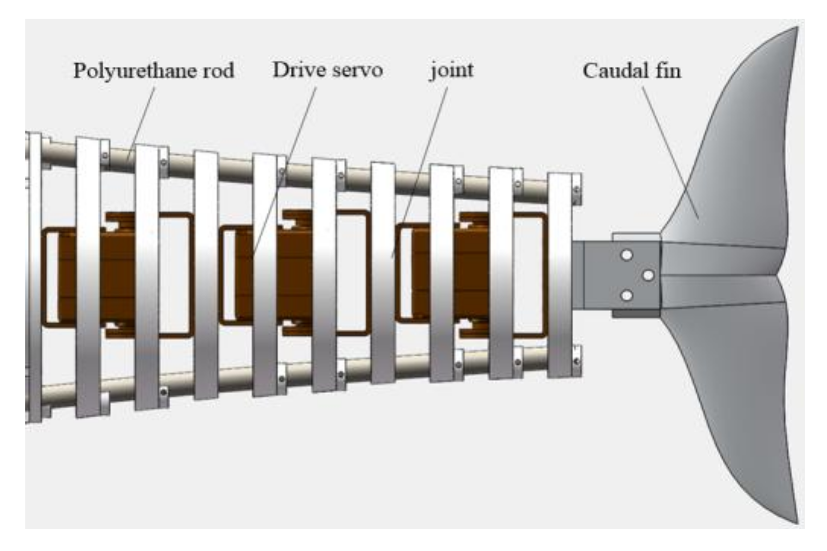
This section is divided into two parts. The tail swing mechanism uses three swing steering gears to drive three active joints, with each pair of active joints containing two driven joints, and two polyurethane rods are used to connect each joint in series. A symmetrical crescent shaped caudal fin is adopted in the structure design of the bionic dolphin caudal fin.
2.1. Tail Swing Mechanism Design
When a dolphin is swimming, its main source of power is the up and down swing of its tail muscles, so the ratio of the total length of the tail swing to the whole body length should be considered in the design process. This ratio not only affects the swimming efficiency and speed of the bionic dolphin, but also its mobility. The mobility of the bionic dolphin increases with the increase of this ratio [14,15].
In addition, the number of tail joints affects the flexibility of the tail: the higher the number of tail joints, the better the flexibility of the tail. The bionic dolphin tail swing mechanism designed is shown in Figure 1. It includes three swing steering gears, nine swing joints, and two flexible spines. The function of the flexible spine is to provide support for the swing of the dolphin’s tail joints. In addition, the flexible spine is elastic and can also play a role in energy storage. When the bionic dolphin is starting or accelerating, it stores excess energy in the flexible spine of each joint. When it enters a stable operation stage, the energy stored in the flexible spine is released, which can improve the energy utilization rate and endurance of the bionic dolphin [16].
The flexible spine is very important for the swing of the bionic dolphin tail. The flexible spine must meet the requirements of a circular cross-section, flexible body, and curved deformation under force [17]. According to the above conditions, there are the following choices for flexible spine materials:
- Spring: Spring has good elasticity and flexibility. However, it is difficult to control the spring when it deforms in the axial direction;
- Silicone tube: The elasticity of silicone tube is good, but its flexibility is insufficient, and it is easy to break;
- Polyurethane rod: Polyurethane rod is a new type of polymer material with good elasticity and flexibility. When the polyurethane rod deforms, the axial deformation is small and easy to control.
Therefore, the flexible spine material of the bionic dolphin’s tail is a polyurethane rod.
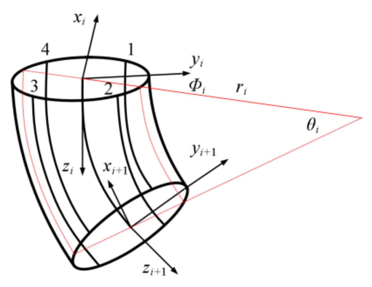
The segmental constant curvature method is used to analyze the flexible spine. The flexible spine is divided into small arcs. The bending posture of each central arc is determined by the following parameters: The radius of curvature , curvature angle , and plane angle . The flexible spine is assumed to be in the same plane when bending, there is = 0°. The coordinate system is and on the small arc of segment . The schematic diagram is shown in Figure 2.
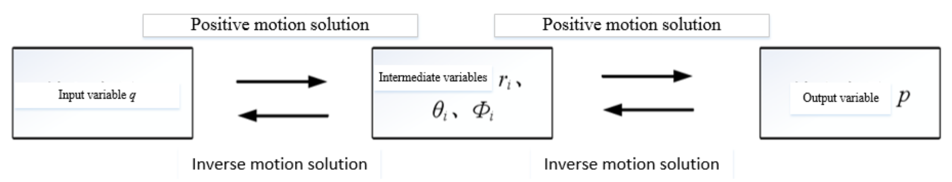
There are two satellite coordinate systems in the upper and lower planes respectively. The origin of the coordinates is the intersection and of the central arc and the upper and lower planes. The and axis remain tangent to the central arc, and the directions are consistent with the section’s directions. The and coincide with the upper and lower sections respectively. The directions of the and axis are judged by the right-hand rule. The input variable is the steering angle . The intermediate variables are the three central arcs of the flexible spine. The output variable is the pose of the central arc of the flexible spine. The relationship among them is shown in Figure 3.
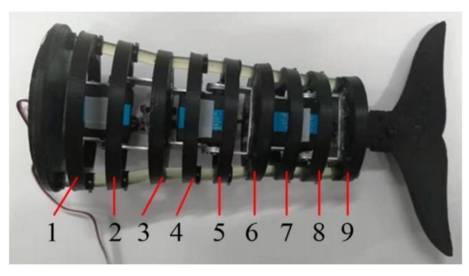
There are two types of joints in the tail of the bionic dolphin. The joints directly connected to the steering gear are called active joints. The joints not directly connected to the steering gear are called driven joints. There are three active joints and six driven joints. The driven joints are fixed to the flexible spine by bolts. The oval joints are evenly distributed on the two flexible spine. Its shape is an ellipse. The size of the oval joint increases from the tail to the head which can make the tail of the bionic dolphin closer to the shape of the real dolphin.
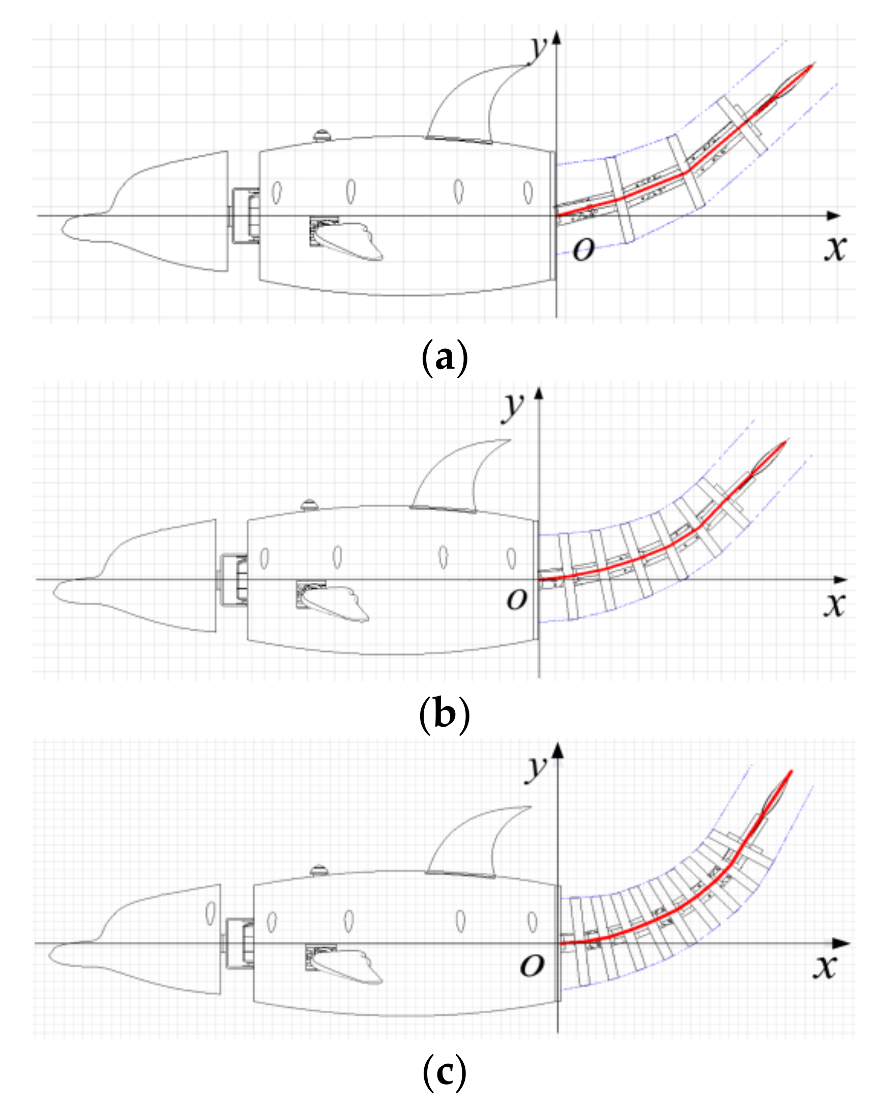
When the three steering gears at the bionic dolphin’s tail move, the active joints are forced to generate a bending moment and drive the flexible spine to bend. As shown in Figure 4, different numbers of driven joints produce different bending curves. When there is no driven joint, the generated curve is a broken line in Figure 4a. When three driven joints are added on the basis of the three active joints, the curve formed during the tail swing in Figure 4b is gradually closer to the fish body wave curve of the real dolphin movement. When six driven joints are added on the basis of the three active joints, the tail swing curve of the bionic dolphin in Figure 4c is very close to the body wave curve of the real dolphin.
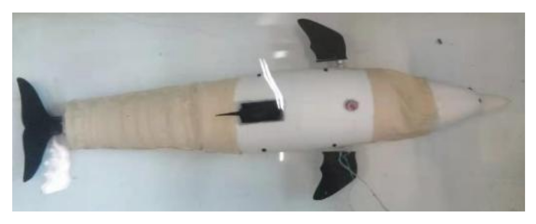
Therefore, the number of driven joints at the tail of the bionic dolphin is selected as six by considering the swing space of the tail. The physical map is shown in Figure 5.
2.2. Bionic Dolphin Tail Fin Structure Design
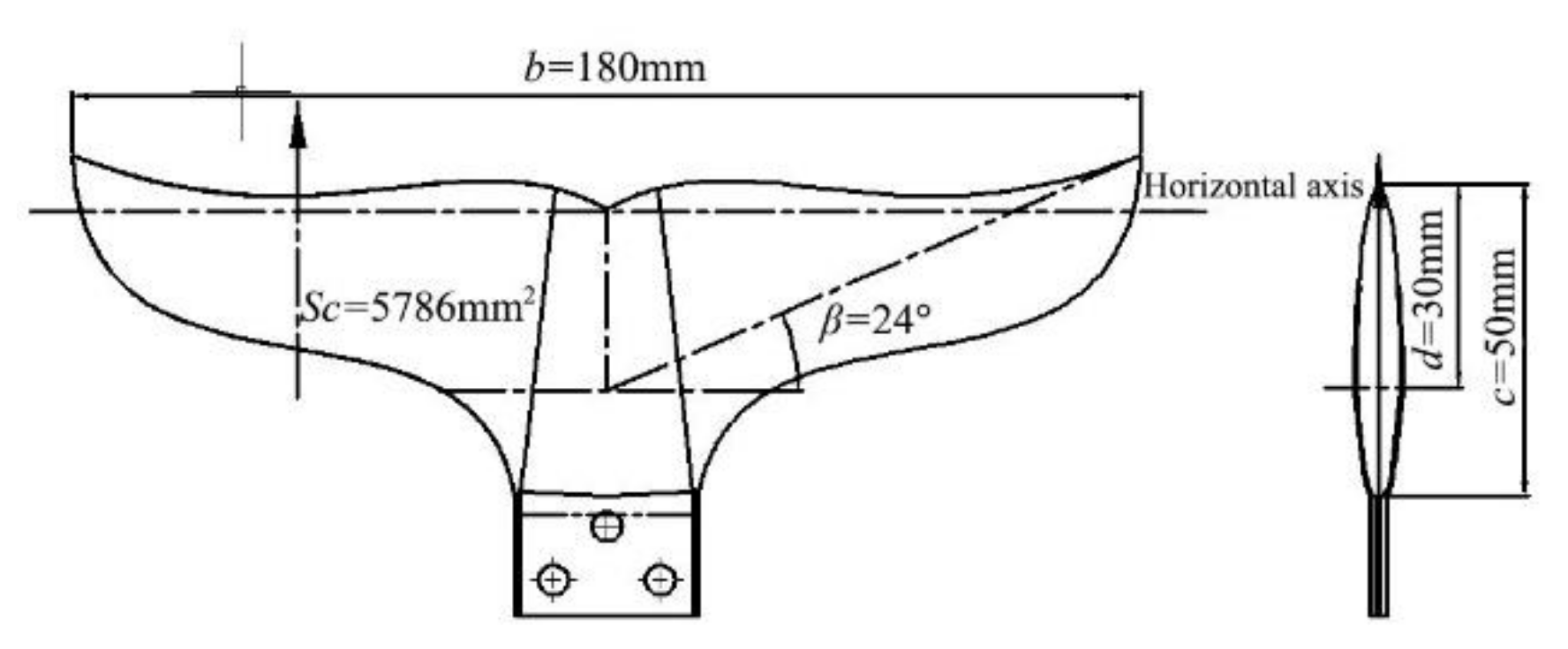
The typical shape of the tail fin of the tuna family mainly includes two kinds of crescent-shaped tail fin and crooked tail. The tail fin of a dolphin belongs to the crescent-shaped tail fin [18]. The symmetrical crescent-shaped tail fin has its own advantages. It not only has a relatively large spread, but also has a blunt arc-shaped front edge and a relatively sharp rear edge, which will cause front-edge suction. This shape greatly reduces the resistance of water to it when it swims in the water. In addition, the symmetrical crescent-shaped tail fin also helps to balance the force in the vertical direction. It makes the dolphins more stable in the vertical direction while swimming in the water [19]. The structure design of the caudal fin adopts a symmetrical crescent-shaped caudal fin. The parameter diagram is shown in Figure 6.
Several important parameters of the tail fin determine the propulsion and efficiency of the bionic dolphin’s tail fin. Therefore, the value range of these parameters must be strictly controlled when designing the shape of the tail fin. These reasonable parameters can make the designed bionic dolphin achieve a good swimming effect [20]. Several design parameters of the tail fin are shown below.
- Aspect ratio . The aspect ratio mainly affects the efficiency of the swing and propulsion of the bionic dolphin’s tail, and its calculation formula is shown in Equation (1). The aspect ratio of the tail fin of different species is slightly different, and the aspect ratio of the dolphin is between 4.5 and 7.2. Through considering the relationship between the propulsion efficiency and the propulsion force, the aspect ratio of the bionic dolphin is selected as 5.6.where is the tail fin spread in millimeters and is the caudal fin area in square millimeters.
- Swept angle . In theory, it can be known that the sharper the trailing edge of the tail fin, the easier it is for the tail vortex to fall off. While the bionic dolphin is swimming, the drag on the tail fin decreases as decreases. Through considering the shape of the actual dolphin tail fin and the tail fin’s area, the value of the swept angle is selected as 24°.
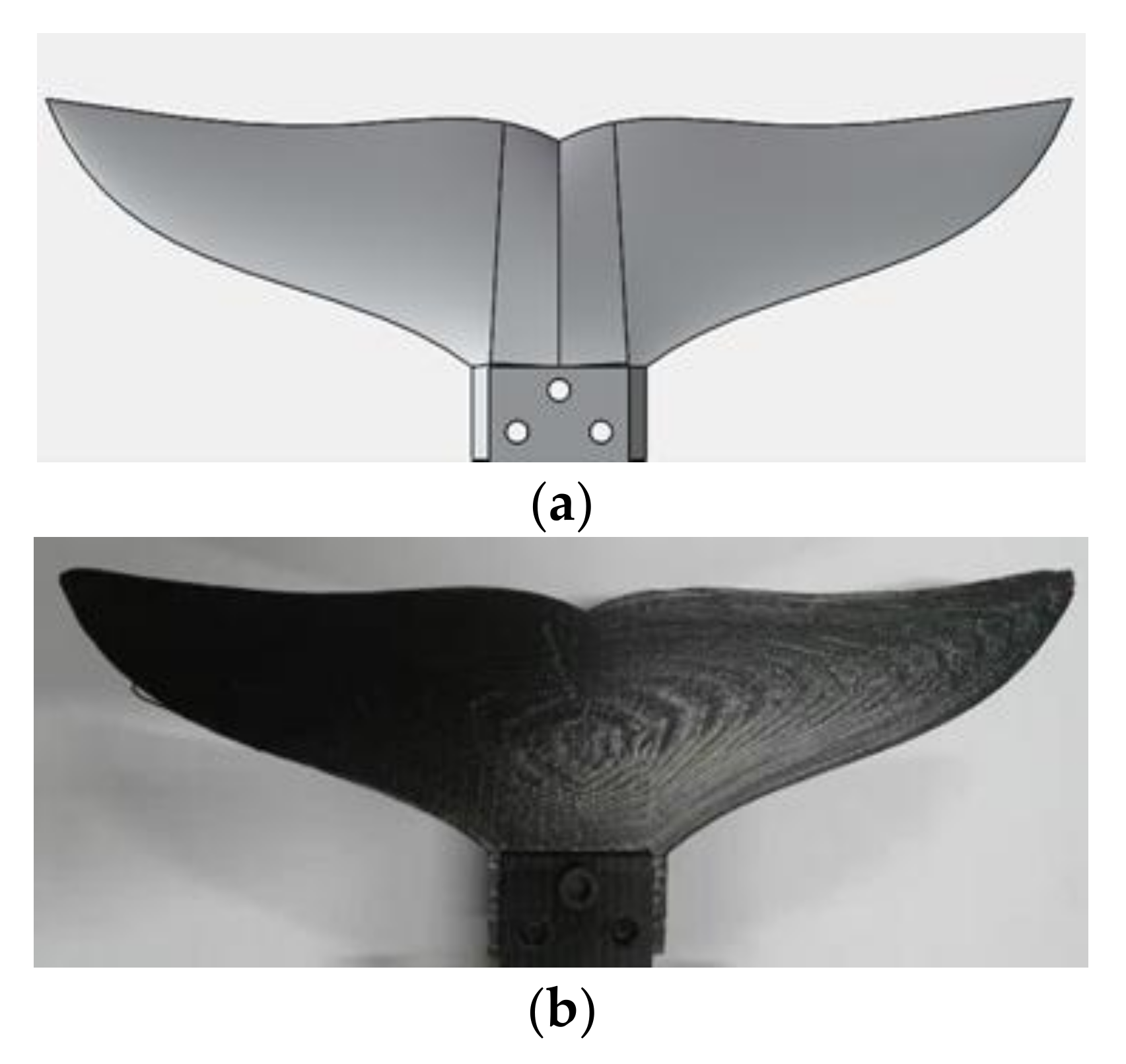
- Tail fin’s stiffness . As the stiffness increases, the propulsion efficiency and propulsion force generated by the tail fin swing are greater. Because the designed tail fin shape is a curved shape, it was decided to use 3D printing technology to process it. The material used for the tail fin is photosensitive resin, which has very high strength and rigidity. But the disadvantage is that the cost is relatively high.
- Strouhal number . This parameter affects the motion posture of the dolphin’s tail wake, and its specific formula is shown in Equation (2). When the propulsion efficiency is the highest, it is between 0.3 and 0.4.where is the caudal fin swing frequency around the sagittal axis in Hertz, is the trailing edge swing of caudal fin in millimeters and is the average speed of fish in meters per second.
3. Kinematic Analysis and Swing Curve Simulation of Bionic Dolphin Tail Mechanism Driven by Servos
This section is divided into kinematic analysis and swing curve simulation of the bionic dolphin tail mechanism. Through analyzing the energy conversion process of the tail swing of the bionic dolphin and applying the kinetic energy mapping principle, the relationship between the swimming speed and the tail servos was calculated. The three factors of the tail servos are swing amplitude, frequency, and phase difference. On this basis, the swing process of the bionic dolphin tail mechanism was simulated in Adams software and then Matlab software was used to fit the tail swing curve.
3.1. Kinematic Analysis of Bionic Dolphin Tail Mechanism Driven by Servos
For the bionic dolphin driven by multiple servos, its tail is driven by three servos to provide power for the whole bionic dolphin to swim forward. In a tail swing cycle, the battery energy is output by a steering gear, which is mainly converted into three parts. One part is converted into the kinetic energy of the surrounding water body. The second part is the circuit loss. The last part is converted into the kinetic energy of the bionic dolphin swimming [21].
The accelerating swimming process of the bionic dolphin is divided into tail swing cycles. In one tail swing cycle, the output power of the tail steering gear is converted into kinetic energy of the robot dolphin, and the proportion is recorded as . At the end of each swing cycle, the bionic Dolphin will increase a velocity .
According to the regular pattern of the dolphin’s tail swing, the kinematic equation of its tail swing angle can be obtained as follows.
where is the tail swing angle in radians and ω is the angular velocity in radians per second.
The three servos of the bionic dolphin’s tail are connected in turn. The three swing angles are assumed to be the same. The angular velocity of the tail fin swing can be obtained with Equation (3).
It can be seen that in a swing cycle, the kinetic energy reaches the maximum when or . The maximum kinetic energy is defined as the characteristic kinetic energy, which is recorded as . The characteristic kinetic energy of the three servos is calculated respectively.
where is one servo mass in kilogram, , , and are the joint centroid velocity in meters per second, , , and are the moment of inertia of mass center in kilogram times meter, and , , and are the angular velocity in radians per second.
The calculation formula of centroid velocity is shown in Equation (6).
The calculation formula of the moment of inertia is shown in Equation (7).
In the formula, ; ; .
The calculation formula of the negative maximum angular velocity of the servos is shown in Equation (8).
In the same way, the maximum angular velocity of the servos can be obtained when it swings in the positive direction. In a movement cycle, whether the tail fin moves downward or upward, part of the energy generated by the tail rudder will be converted into forward power.
In order to simplify the calculation process, let . Simultaneously, Equations (5)–(9) leads to Equation (10).
where is the bionic dolphin mass in kilograms, is the increasing speed of the cycle in meters per second, is the mass of the steering gear in kilograms, is the length of the steering gear in meters, is the oscillation frequency in Hertz(), and is the maximum swing angle in radians.
When the tail of the bionic dolphin goes through swing cycles, the speed reaches the maximum, the kinetic energy does not increase, and it reaches a certain speed value.
Equation (11) gives the energy conversion formula of swing cycles. Because one cycle and the variables that can be set as input are the energy conversion coefficients of the corresponding cycles, when the robot dolphin reaches the maximum speed, the energy conversion coefficient is zero, which is expanded from Equation (11) to Equation (12).
According to Equation (12) and , Equations (13) and (14) can be deduced.
In Equation (14), represents the velocity that enters the steady state after a period of time given a swing amplitude and swing angular velocity, which is the general motion model of discrete kinematic. Equation (14) is a simplified model and is a total conversion scale factor.
3.2. Kinetic Energy Mapping Principle and Kinematic Nonlinear Characteristic Equation
When the amplitude and frequency are given, the bionic dolphin reaches a fixed speed after tail swing cycles. When the bionic dolphin enters a stable swimming state, its characteristic kinetic energy and average kinetic energy are extracted. The ratio between them is the kinetic energy mapping coefficient, and the relationship between them is the kinetic energy mapping principle. The motion equation of the bionic dolphin tail is shown in Equation (15).
where is the particle wave function, is the maximum swing of caudal fin in radians, and is the swing angle frequency in Hertz.
The particle wave function can be expressed by Equation (16).
According to Equations (15) and (16), the basic kinetic energy mapping equation and the discrete kinematic nonlinear characteristic equation based on swing frequency control are obtained. As shown in Equations (17) and (18).
where represents the mass of the bionic dolphin in kilogram, represents the velocity that enters the steady state after a period of time in meters per second and corresponds to in Equation (14). is the kinetic energy mapping coefficient that depends on the hydrodynamic characteristics and the surrounding water environment, corresponds to in Equation (13). is the characteristic kinetic energy in joules. where is the steady-state average velocity in samples of oscillation period with time in meters per second, is the kinetic energy mapping coefficient in samples of oscillation period with time , corresponds to in the previous section, is the input swing angular velocity in radians per second, and is the duration of oscillation period in seconds.
Equation (18) is mainly based on energy conversion and motion feature extraction. The kinetic energy mapping coefficient is measured and the swimming speed of the bionic dolphin is controlled by the input angular velocity signal.
3.3. Simulation of Tail Swing Curve of Bionic Dolphin by Servos
The tail of this bionic dolphin is driven by three servos to provide power for the bionic dolphin to swim forward. There are seven groups in this section, and their classification is based on the number of driving servos and the phase difference, as shown in Table 1. The servos from tail to head are numbered 1, 2, and 3. When the servo 2 or 3 is driven, servo 1 follows the tail swing even though it is not driven, so it is interpreted as follows.
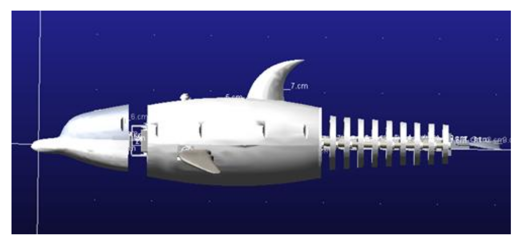
These seven driving schemes were simulated in Adams software, as shown in Figure 8. In order to make the simulation easier and more convenient, all parts that are not related to motion in the bionic dolphin model are removed.
According to the number of different driving servos and whether there is a phase difference between each adjacent servo, each situation was simulated in Adams software. The three active joints at the tail of the bionic dolphin were used as sampling points, and the collected data with group number 111 are shown in Table 2. In order to better compare the tail swing curves of the nine joint and three joint bionic dolphin, the nine joint data collection points were also set up. The data collection is shown in Table 3.
Adams simulation of the above seven driving schemes was carried out, and then the respective fish body wave curve was fitted by Matlab software, which can compare the fish body waves formed by different driving schemes with the real situation.
When the number of driven servos is different and when there is a phase difference between adjacent servos, the fish body wave fitting curve formed by the swing of the bionic dolphin’s tail is different. The difference in the number of joints in the tail of the bionic dolphin also affect the fish body wave curve formed. The driving mode with only one servo is shown in Figure 9. The driving mode with two servos is shown in Figure 10. And the driving mode with three servos is shown in Figure 11.
According to Figure 9, Figure 10 and Figure 11, when the number of driving servos is three and there is a phase difference between their swings, the resulting fish body wave curve is more in line with the dolphin S-shaped swimming curve.
When two flexible spines and six driven joints are added to the tail of the bionic dolphin, the tail swing curve of the bionic dolphin is more in line with the real fish body wave curve, as shown in Figure 12. Therefore, the nine joint flexible swinging tail of the bionic dolphin is more reasonable than the three joint bionic dolphin swinging tail. The rationality of the designed bionic dolphin was verified, and the foundation was laid for the next experiment.
The tail swing curve in Figure 13 was obtained by fitting the curve in Figure 12 through the Matlab software. The purpose of the fitting is to consider that the real dolphin is affected by the degree of body bending when swimming.
It can be seen from Figure 9, Figure 10, Figure 11, Figure 12 and Figure 13 that when the three servos at the tail of the bionic dolphin are driven and work with a uniform phase difference, the bionic dolphin has a better fish body wave curve, which can achieve a better S-type BCF propulsion effect and keep the entire bionic dolphin within the envelope of the fish body.
4. Experimental Study
The tail swing mechanism of the bionic dolphin is studied in this section. Firstly, the control model was constructed, and the simulation analysis of the parameters of control variables was completed. Then, the platform of the dolphin experiment prototype was built. Through the comparative experimental study of the body wave curve of the bionic dolphin fish, it was concluded that it can fit the body wave curve of fish well. Then the effects of tail swing phase difference, swing amplitude and swing frequency on dolphin speed were studied, and the relative relationship was obtained. Finally, the conclusion was drawn that when the bionic Dolphin = 0.3π, = 4 Hz and = 100 mm, the maximum swimming speed of the bionic dolphin is 0.75 m/s.
4.1. CPG Control Analysis of Bionic Dolphins Based on Kane Dynamic Model
In order to control the amplitude, the phase difference, and the frequency of the tail swing of the bionic dolphin, a CPG control model is used to control the three parameters separately [22,23]. It is assumed that there are joints of bionic dolphin. From the head to the caudal fin of the robot dolphin, the joint is 0 to . A coordinate system is established as .
The coordinate system is established in the tail joint, where is located at the center of the tail joint. is parallel to the axis of the steering gear and is perpendicular to the plane of the steering gear. Then the right-hand rule is used to determine the direction of . The length and mass of the bionic dolphin tail actuator are and , respectively. The center of gravity of the bionic dolphin tail joint is , and the geometric center is . The mass of the tail joint is assumed to be continuous and uniform, so the two points coincide. is the angle between the joint and the joint, is the rotation matrix from the coordinate system to the coordinate system , as shown in Equation (20).
The position vector is the origin of the tail joint to the origin of the world coordinate system , as shown in Equation (21).
The position vector of the center of mass of the tail joint is obtained, as shown in Equation (22).
When the bionic dolphin swims in the water, each joint of the tail provides forward power for it by swinging. The angular velocity and angular acceleration of each joint at the tail are shown in Equation (23).
The velocity and acceleration of the center of mass of the dolphin tail joint are shown in Equation (24).
When the bionic dolphin swims in the water, it is assumed that the buoyancy and gravity in the vertical direction are in balance. Then the generalized active force and inertial force of the bionic dolphin are calculated. The swimming speed and acceleration of the bionic dolphin are shown in Equation (25).
At the same time, because the swimming of the bionic dolphin drives the surrounding fluid to move, it is necessary to calculate the additional mass effect, which is expressed by Equation (26).
where is the inertial force due to added mass in Newton, is the moment of inertia due to added mass in Newton meter, is the skew symmetric matrix, is the form of an additional mass matrix in the local coordinate system .
The resistance of the bionic dolphin swimming in water is divided into pressure resistance and friction resistance. The calculation method with a large Reynolds number is shown in Equation (27).
where is the density in kilogram per cubic meter, is the relative velocity of the joint in meters per second, are the drag coefficients in Y and X directions, are the effective area of x-axis and y-axis in square meters.
The resistance moment of bionic dolphin in water is shown in Equation (28).
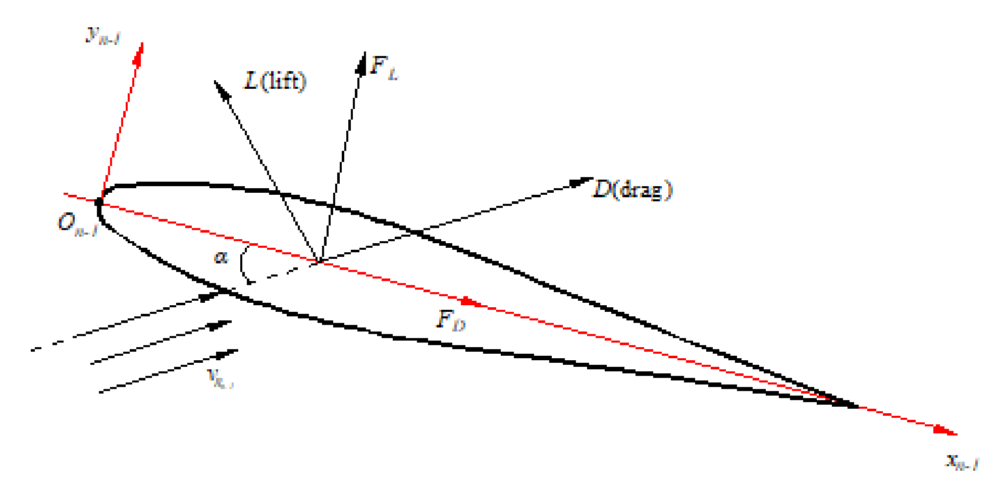
When the bionic dolphin swims in the water, the caudal fin is affected by the reaction force of the water. The force diagram is shown in Figure 14.
Because the velocity of the liquid flowing through the upper and lower surface of the caudal fin is different, an upward lift is generated. The expressions of lift and drag are shown in Equation (29).
The angle between the axis of the caudal fin and the direction of the flow velocity is . The equation of lift and resistance in the local coordinate system of the tail joint is shown in Equation (30).
The moment of the caudal fin is calculated as shown in Equation (31).
When the tail joint of the bionic dolphin swings, the torque provided by the joint is , which is expressed in the local coordinate system . is the size in the local coordinate system .
Through the above analysis and derivation, the force and moment of the bionic dolphin tail joint are calculated, as shown in Equation (33).
The Kane method is needed to calculate the deflection velocity and angular velocity when the generalized inertial force of the system is calculated, as shown in Equation (34).
where is the generalized inertial force of the system in Newton, is the joint forces in Newton, and is the action moment of joint in Newton meters.
The generalized inertial force generated by the additional mass effect is shown in Equation (35).
When the Kane method is used to calculate the generalized active force, it is necessary to sum the scalar product of the active force on each particle and the partial velocity of the particle. The formula for calculating the generalized active force on the bionic dolphin is shown in Equation (36).
The Kane equation of the system is established, as shown in Equation (37).
The Kane dynamic model is used to verify the relevant parameters in the CPG control model. The solution of Equation (37) can obtain the relevant parameters such as the amplitude, frequency, and phase difference of the tail swing of the bionic dolphin. Then the signal is input into the system in the CPG control model. To determine the amplitude of the bionic dolphin swing. The relevant simulation parameters are shown in Table 4.
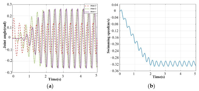
The driving frequency of CPG is 2 Hz and the phase difference between joints is . The swing amplitude of each joint was 0.26 rad, 0.26 rad and 0.12 rad respectively. The driving signals of the three joints of the bionic dolphin and the swimming speed of the bionic dolphin in the water are calculated in Matlab software, as shown in Figure 15.
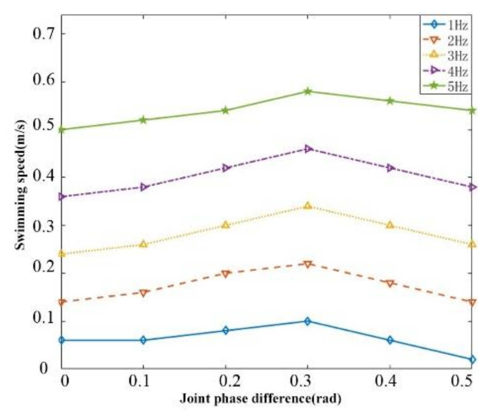
It can be seen from Figure 15 that the swimming speed of the bionic dolphin reaches a maximum of 0.32 m/s after 2 s acceleration in the water. When the bionic dolphin’s tail swing frequency and phase difference are set in the simulation, the speed change diagram of the bionic dolphin swimming in the water is obtained, as shown in Figure 16.
According to Figure 16, the swimming speed of the bionic dolphin increases with the increase of the tail swing frequency. When the frequency is kept constant, the phase difference of the joint swing increases gradually, and the speed of the joint will increase first and then decrease gradually. When φ = 0.3π, the speed reaches the maximum.
4.2. Curve Fitting Experiment of Bionic Dolphin Tail Based on Steering Gear Drive
The above simulation analysis of the fish body wave of the bionic dolphin has been carried out, and it is concluded that when there is a phase difference in a steering gear driven, the fitting curve of the tail of the bionic dolphin is more in line with the real dolphin fish body wave curve. In order to verify the rationality of the designed bionic dolphin prototype, the test obtained the fish body wave fitted when there are different numbers of driving servos and phase differences between the servos.
The model of tail drive steering gear used in the bionic dolphin experimental prototype is LDX-218 and the torque is 32 kg·cm. It is powered by an adjustable DC voltage stabilized power supply or 2200 mA·h lithium battery, and controlled by STM32F405 system development board.
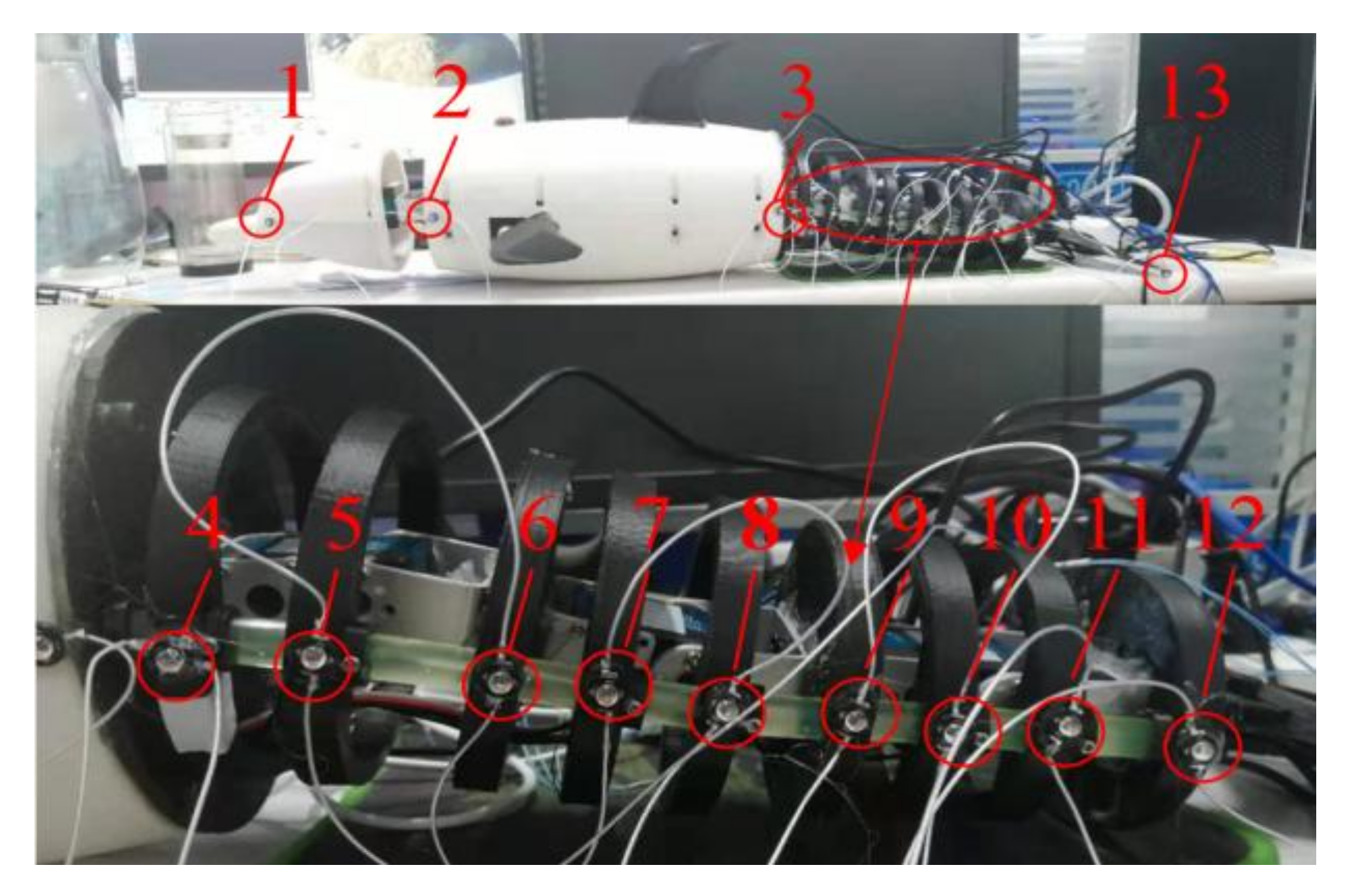
In the experiment, the body part of the dolphin prototype was fixed on the test bench, and the head and tail were suspended. Small infrared lamp beads were pasted on the head, body, tail swing joint and tail fin of dolphin prototype as infrared marking points. The infrared camera was placed on its side to capture the motion state of the dolphin prototype, as shown in Figure 17.
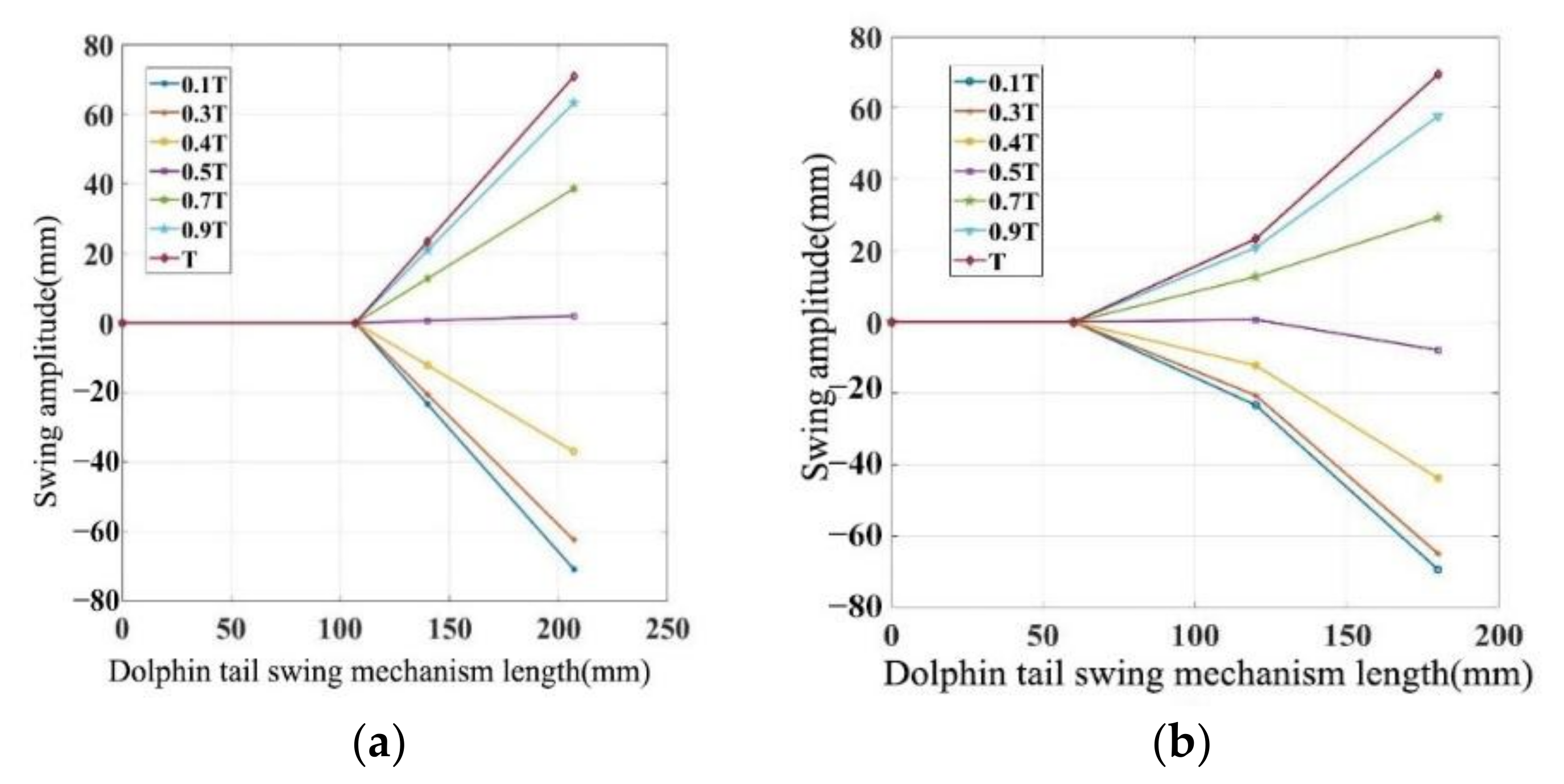
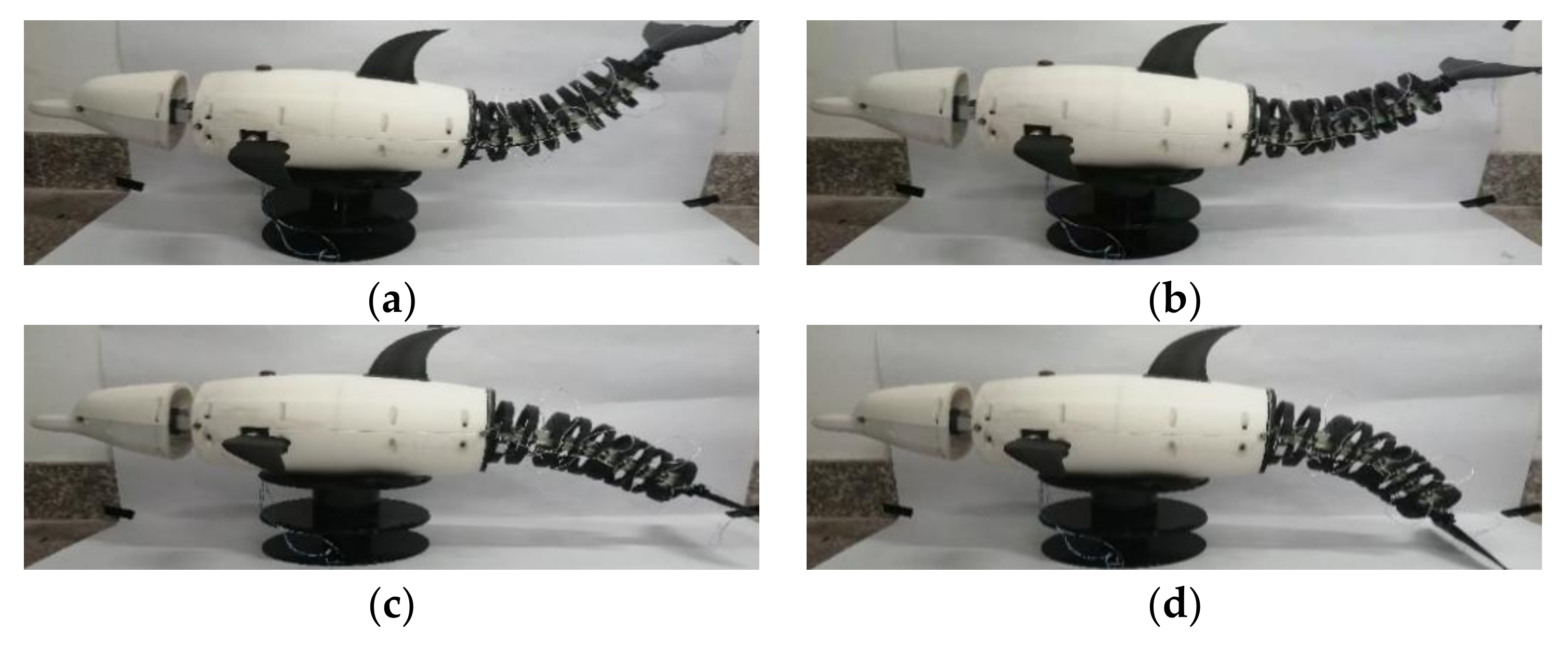
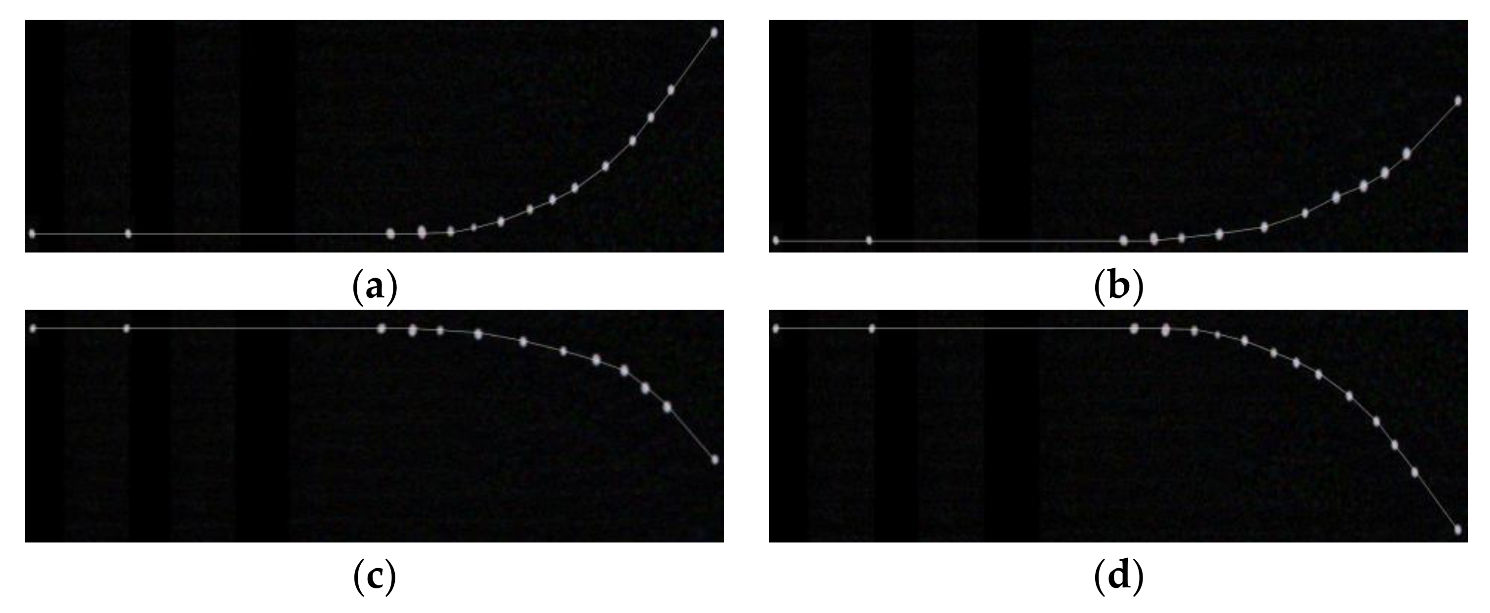
During the experiment, the tail of the dolphin was controlled to swing, and the camera was used to record the tail posture of the dolphin at different times of swing, and the tail swing fitting curve of the dolphin prototype was compared, as shown in Figure 18.
The data were collected by capturing 13 infrared small lamp beads on the dolphin like fuselage. These data were processed in Matlab software and fitted by fish body wave curve. The captured infrared beads are shown in Figure 19.
Meanwhile, in order to better measure the motion curve of the tail swing of the dolphin, a high-precision gyro accelerometer MPU6050 was attached to the three active joints of the tail. The gyroscope transmitted the swing angle, angular acceleration and angular velocity to the upper computer software, and then the real-time position of the tail was calculated based on the joint length and the returned offset angle value. Finally, the swing posture of the bionic dolphin prototype was collected by the LabVIEW video acquisition module.
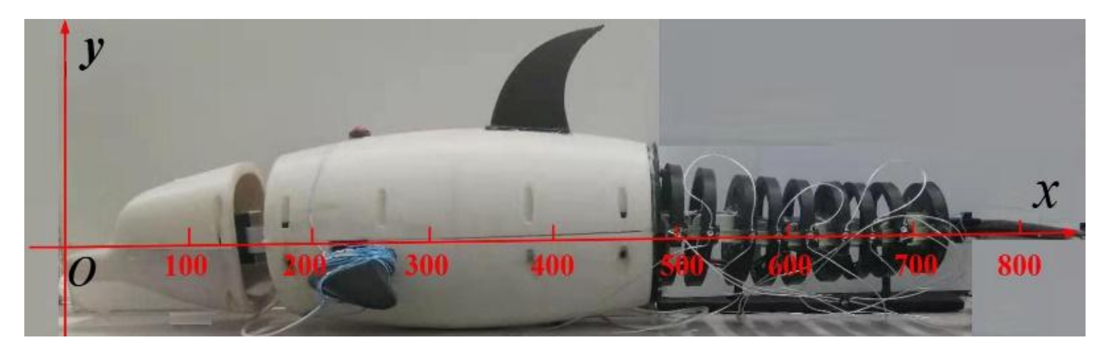
A coordinate system was established for the bionic dolphin prototype, as shown in Figure 20. The abscissa is the center line of the prototype, the leftmost end of the dolphin’s head is the ordinate, and the leftmost end of the dolphin’s mouth is the coordinate origin.
According to the proportional relationship between the two points, the scale function is used to calculate the abscissa and ordinate of each small infrared lamp bead. Because the body and head are not involved in the swing, the ordinate value of the first three points is 0, and the data of other points are shown in Table 5.
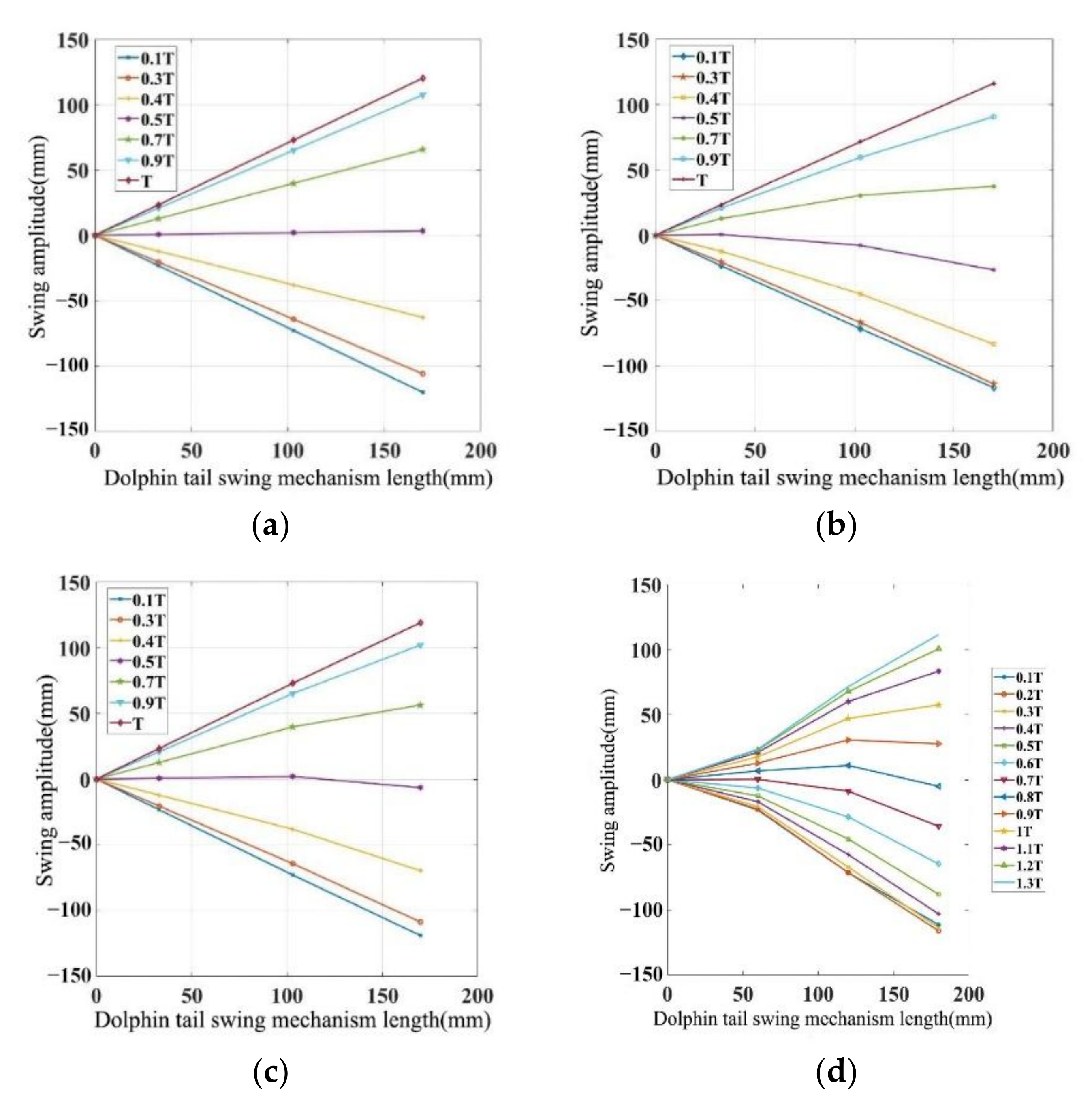
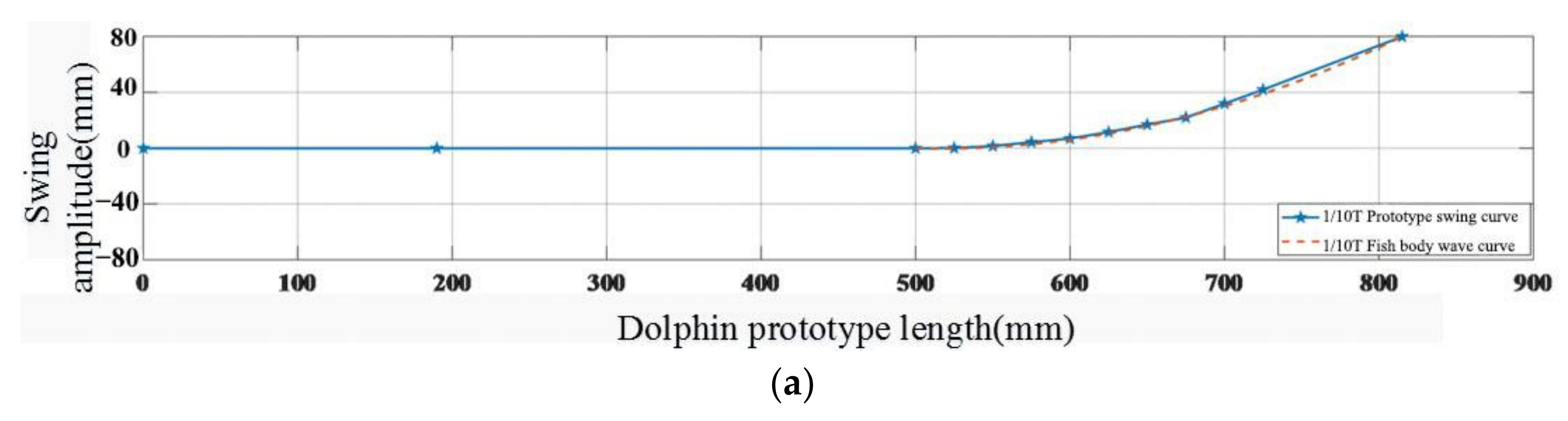
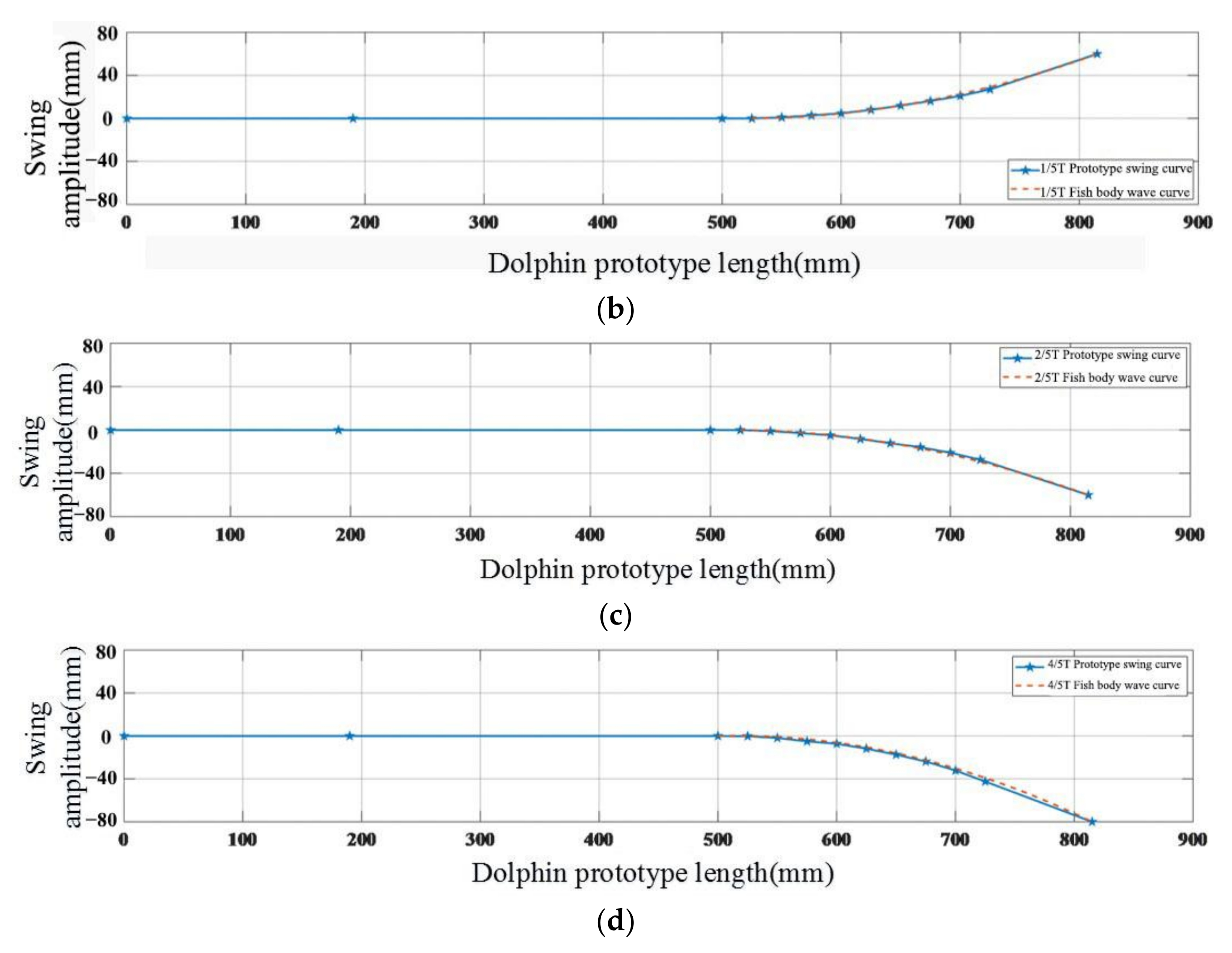
The data in Table 5 and the data collected by the sensor were summarized and calculated to obtain the coordinate value of the fish body wave curve of the dolphin experimental prototype. The fish body wave waveform of the dolphin experimental prototype is obtained with Matlab software, as shown in Figure 21.
It can be seen from Figure 19 and Figure 21 that the swing trend of the joint center line at each characteristic time is consistent with the corresponding point on the simulation curve by controlling different swing phase differences of the bionic dolphin prototype, which can better simulate the swing posture of the dolphin.
4.3. Underwater Tail Swing Experiment Based on Steering Gear Drive
In this section, an underwater cruise experiment was carried out on the bionic dolphin experimental prototype. The influence of tail swing frequency, tail swing amplitude and tail joint swing on the speed of the bionic dolphin experimental prototype were studied by the method of controlling variables.
Because this experiment was carried out in water, water tightness is very important. A natural 0.5 mm elastic rubber skin was used to wrap the experiment prototype, and use waterproof glue for bonding. In the water tightness experiment, it was found that the water tightness of the bionic dolphin experimental prototype in the water was good, as shown in Figure 22.
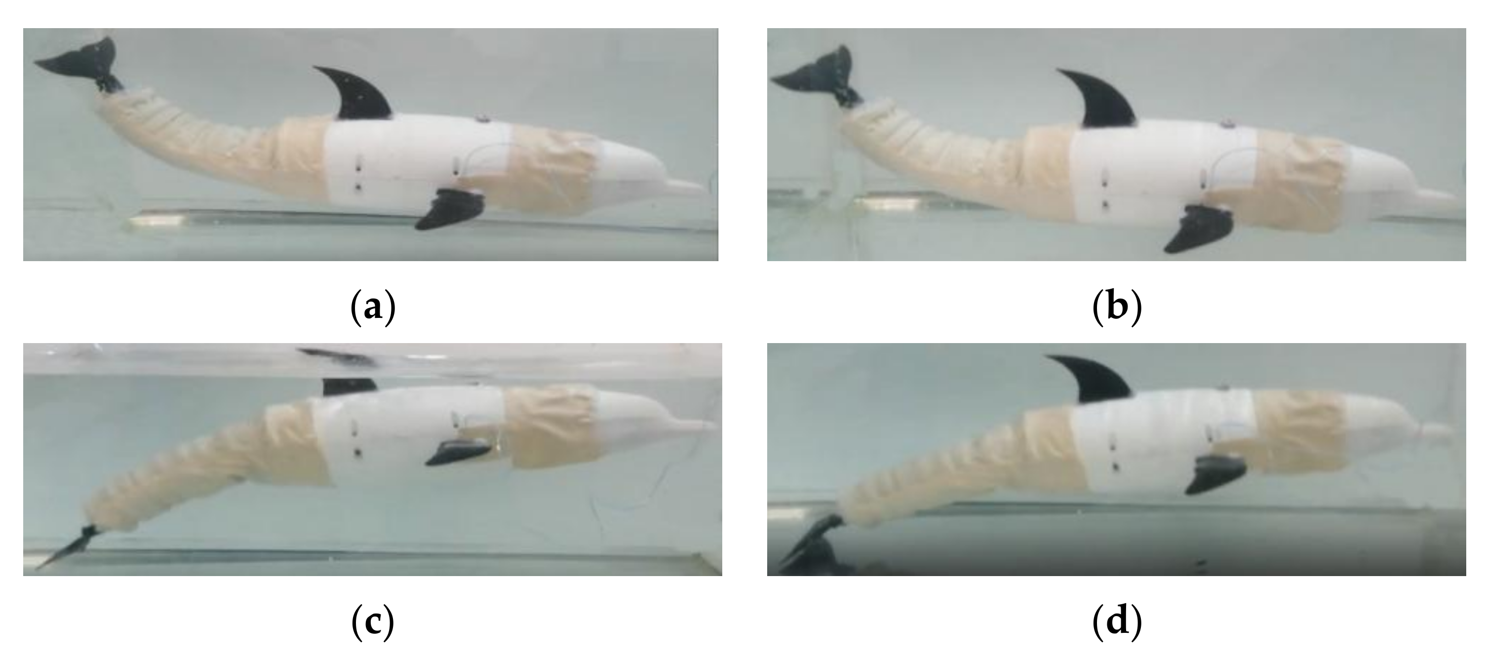
The control parameter is = 1 Hz, = 0.2π. The swimming posture of the bionic dolphin was captured by the camera in real time, and then its swing posture at different times was extracted to obtain the swimming sequence image as shown in Figure 23.
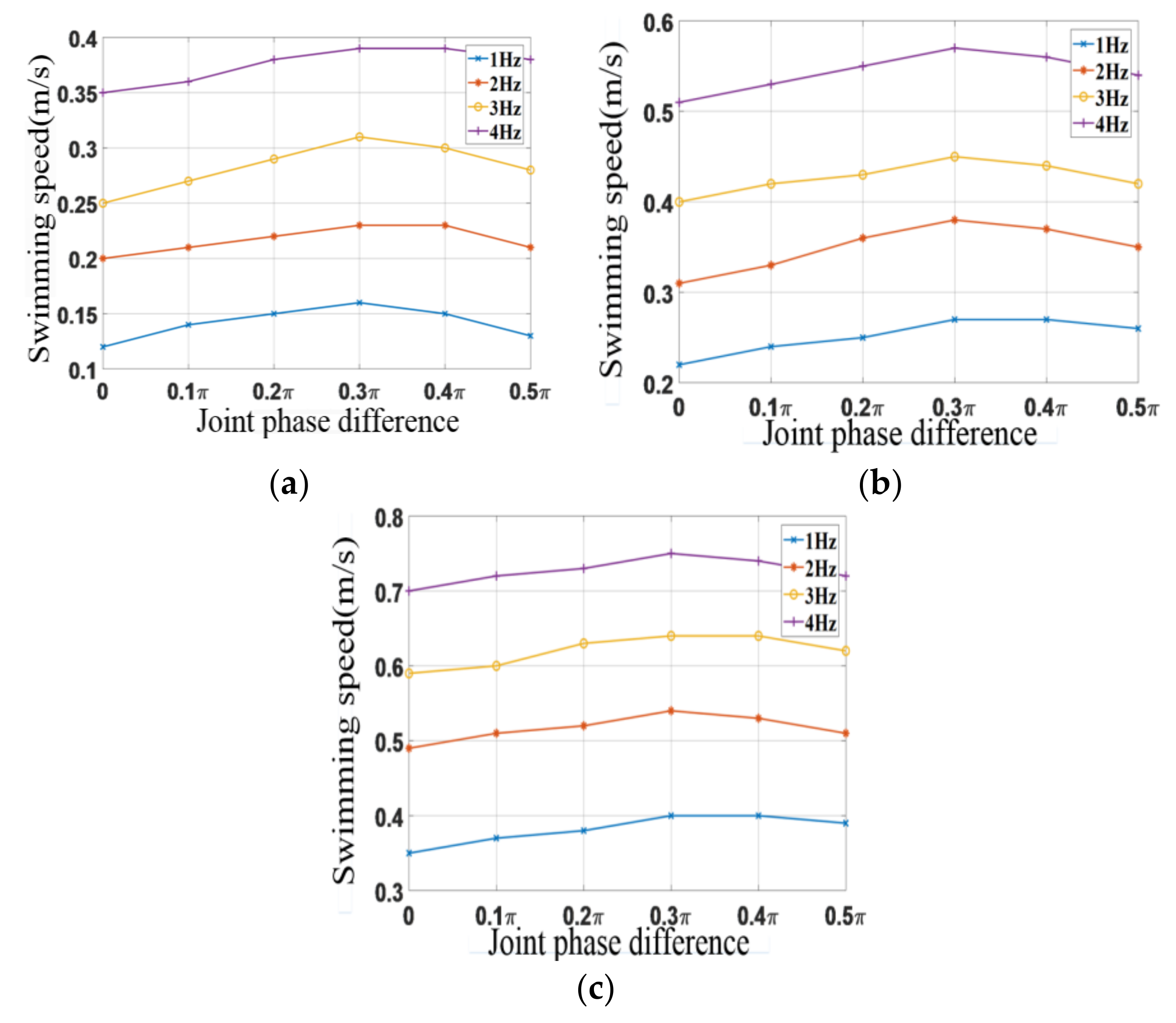
Through controlling the swing, the amplitude of the tail of bionic dolphins is 60 mm, 80 mm, and 100 mm, the experiment is carried out with different phase differences and different frequencies. The swimming speed of the obtained experimental prototype was plotted as a curve, as shown in Figure 24.
It can be seen from Figure 24 that when the swing phase difference and the swing amplitude of the experimental prototype are constant, the swimming speed increases with the increase of the swing frequency of the experimental prototype. When the experimental prototype swing frequency and swing amplitude are constant, the swimming speed of the experimental prototype first increases and then decreases with the increase of the phase difference . When = 4 Hz and = 0.3π, the maximum swimming speed is 0.75 m/s. This is because the experimental prototype is driven by a steering gear, which is limited by the steering gear swing frequency. When the swing frequency continues to increase, the tail swing amplitude cannot swing according to the predetermined amplitude.
5. Conclusions
This article mainly studied a mechanism of the tail swing of a bionic dolphin with a steering gear drive and two flexible spines. The total weight of the bionic dolphin experimental prototype is 2.4 kg and the total length is 815 mm. In order to solve the problem of excessive stiffness of tail swing mechanism caused by the steering gear, two flexible spines were used in series at the tail of the bionic dolphin. Meanwhile, the number of swinging joints of the bionic dolphin tail was increased from three to nine. The rigid joints were changed into flexible joints. Through controlling the different swing frequency, swing amplitude and phase difference of the three driving servos of tail, the different swing posture of the bionic dolphin experimental prototype was realized. The nine joint flexible tail swing mechanism driven by a steering gear had a better tail swing curve than the original three joint rigid tail swing mechanism through analyzing the tail swing curve of the bionic dolphin, which could well simulate the tail swing curve of the real dolphin. When = 4 Hz and = 0.3π, the swimming speed of the bionic dolphin test prototype reaches a maximum of 0.75 m/s.
On the basis of ensuring accuracy, the rationality of the flexible swing mechanism of bionic dolphins is verified by experiment, and the problem of excessive rigidity of the tail swing mechanism caused by the steering gear driving is successfully solved. It provides an experimental basis for the further development of a bionic underwater vehicle.
Author Contributions
All the authors contributed to this paper. Conceptualization, Z.W.; methodology, B.Z.; software, T.W.; resources, B.Z.; data curation, Q.L.; writing—original draft preparation, Z.W.; writing—review and editing, Q.L. All authors have read and agreed to the published version of the manuscript.
Funding
This research was funded by NNSFC (National Natural Science Foundation of China) (Contract name: Research on ultimate bearing capacity and parametric design for the grouted clamps strengthening the partially damaged structure of jacket pipes), grant number 51879063.
Data Availability Statement
Data sharing is not applicable to this article.
Acknowledgments
Throughout the writing of this dissertation, we have received a great deal of support and assistance. This article was funded by NNSFC (National Natural Science Foundation of China). Thanks for our tutors and classmates for their patience and excellent cooperation. The views expressed here were the authors alone.
Conflicts of Interest
The authors declare no conflict of interest.
References
- He, Y.; Huang, Y. The significance of protecting the marine environment in the exploitation of marine resources. Chin. Market 2018, 1, 233–234. [Google Scholar]
- Moynihan, R.; Magsig, B.O. The role of international regimes and courts in clarifying prevention of harm in freshwater and marine environmental protection. Int. Environ. Agreem. Polit. Law Econ. 2020, 20, 649–666. [Google Scholar] [CrossRef]
- Gao, S.; Zhao, L.; Sun, H.H.; Cao, G.X.; Liu, W. Evaluation and Driving Force Analysis of Marine Sustainable Development Based on the Grey Relational Model and Path Analysis. J. Resour. Ecol. 2020, 11, 570–579. [Google Scholar]
- Zheng, Y.H.; Guo, H.D.; Wu, S.C. Analysis of my country’s energy status and its development strategy. City 2018, 1, 35–42. [Google Scholar]
- Zhang, S.; Zhang, A.M.; Cui, P.; Li, T. Simulation of air gun bubble motion in the presence of air gun body based on the finite volume method. Appl. Ocean Res. 2020, 97, 102095. [Google Scholar] [CrossRef]
- Wang, J.C.; Jing, C.L.; Tian, X. The operation and maintenance status of large-scale marine equipment in the United States and its enlightenment to my country. Mar. Sci. 2018, 44, 171–179. [Google Scholar]
- Ren, Y.G.; Liu, B.H.; Ding, Z.J.; Li, Y.; Yang, L.; Hu, X.H. Development status and trends of manned submersibles. J. Ocean Technol. 2018, 37, 114–122. [Google Scholar]
- Liang, J.; Wang, T.; Wen, L. Development of a two-joint robotic fish for real-world exploration. J. Field Robot. 2011, 28, 70–79. [Google Scholar] [CrossRef]
- Hu, Y.Y. Research on the Control System of High-Mobility Bionic Robotic Dolphin Based on STM32. Master’s Thesis, Shenzhen University, Shenzhen, China, 2018. [Google Scholar]
- Xu, D.; Zeng, H.N.; Peng, X. A Stiffness Adjustment Mechanism Based on Negative Work for High-efficient Propulsion of Robotic Fish. J. Bionic Eng. 2018, 15, 270–282. [Google Scholar] [CrossRef]
- Shen, F. Modeling and Control of Bionic Robotic Dolphin and Its Application in Water Quality Monitoring. Master’s Thesis, Graduate School of Chinese Academy of Sciences, Beijing, China, 2012. [Google Scholar]
- Wang, M.; Zhang, Y.L.; Dong, H.F.; Yu, J.Z. Trajectory tracking control of a bionic robotic fish based on iterative learning. Sci. China Inf. Sci. 2020, 63, 505–518. [Google Scholar] [CrossRef]
- Wang, S.Y.; Zhu, J.; Wang, X.J.; Li, Q.F.; Zhu, H.Y.; Zhou, R. Optimization and simulation of a bionic fish tail driving system based on linear hypocycloid with hydrodynamics. Adv. Mech. Eng. 2017, 9, 975–991. [Google Scholar] [CrossRef] [Green Version]
- Techet, A.H.; Hover, F.S.; Triantafyllou, M.S. Separation and Turbulence Control in Biomimetic Flows. Flow Turbul. Combust. 2003, 71, 105–118. [Google Scholar] [CrossRef]
- Liu, J.; Hu, H. Biological Inspiration: From Carangiform Fish to Multi-Joint Robotic Fish. J. Bionic Eng. 2010, 7, 35–48. [Google Scholar] [CrossRef]
- Wang, Y.W.; Yu, K.; Yan, Y.C. Research status and development trend of BCF propulsion model bionic robotic fish. Micro Special Motor 2016, 44, 75–80. [Google Scholar]
- Peng, Z.C. Motion Simulation of Fish-Like Robot. Master’s Thesis, Harbin Engineering University, Harbin, China, 2003. [Google Scholar]
- Liu, Y.X.; Liu, J.K.; Chen, W.S. Development and experimental study of a new type of two-joint robotic fish. Ship Eng. 2008, 30, 28–31. [Google Scholar]
- Yang, Y.; Wang, J.; Wu, Z. Fault-Tolerant Control of a CPG-Governed Robotic Fish. Engineering 2018, 4, 861–869. [Google Scholar] [CrossRef]
- Osama, E.; Christopher, H.; Darryl, W.H. Characterization of acoustic detection efficiency using a gliding robotic fish as a mobile receiver platform. Anim. Biotelem. 2020, 8, 260–272. [Google Scholar]
- Ren, G. Research on Kinematics and Control Method of Robot Dolphin Propulsion System. Master’s Thesis, Beijing Institute of Technology, Beijing, China, 2015. [Google Scholar]
- Xie, F.G.; Zhong, Y.; Du, R.X. Central Pattern Generator (CPG) Control of a Biomimetic Robot Fish for Multimodal Swimming. J. Bionic Eng. 2019, 16, 222–234. [Google Scholar] [CrossRef]
- Sheng, F.; Cao, Z.Q.; Xu, D.; Zhou, C. Dynamic modeling and speed optimization method of robotic dolphin based on Kane method. Acta Autom. Sin. 2012, 38, 1247–1256. [Google Scholar] [CrossRef]
Figure 1.
Bionic dolphin flexible tail swing mechanism.

Figure 2.
Flexible fish body segmented constant curvature model.

Figure 3.
The mapping relationship of each group of variables.

Figure 4.
Schematic diagram of different numbers of joints: (a) three joints of the dolphin tail; (b) six joints of the dolphin tail; (c) nine joints of the dolphin tail.
Figure 4.
Schematic diagram of different numbers of joints: (a) three joints of the dolphin tail; (b) six joints of the dolphin tail; (c) nine joints of the dolphin tail.

Figure 5.
Physical picture of nine joints of dolphin’s tail. 1, 2, 4, 5, 7, 8—swing fishtail follower joint. 3, 6, 9—swing fishtail active joint.
Figure 5.
Physical picture of nine joints of dolphin’s tail. 1, 2, 4, 5, 7, 8—swing fishtail follower joint. 3, 6, 9—swing fishtail active joint.

Figure 6.
Parameters of the bionic dolphin’s tail fin.

Figure 7.
Schematic diagram of tail fin structure: (a) 3D model of caudal fin; (b) real picture of the caudal fin.
Figure 7.
Schematic diagram of tail fin structure: (a) 3D model of caudal fin; (b) real picture of the caudal fin.

Figure 8.
Adams simulation of the tail swing.

Figure 9.
The amplitude envelope of seven driving modes: 001—servo 1 drive.

Figure 10.
The amplitude envelope of seven driving modes: (a) 010—servo 2 drives the servo 1 to follow; (b) 011—servo 1, 2 has phase difference drive.
Figure 10.
The amplitude envelope of seven driving modes: (a) 010—servo 2 drives the servo 1 to follow; (b) 011—servo 1, 2 has phase difference drive.

Figure 11.
The amplitude envelope of seven driving modes: (a) 100—only servo 3 drive; (b) 101— only servos 1, 3 have phase difference drive; (c) 110—only servo 2, 3 drive; (d) 111—servo 1, 2, 3 have phase difference drive.
Figure 11.
The amplitude envelope of seven driving modes: (a) 100—only servo 3 drive; (b) 101— only servos 1, 3 have phase difference drive; (c) 110—only servo 2, 3 drive; (d) 111—servo 1, 2, 3 have phase difference drive.

Figure 12.
Group 111 nine joint fitting curve.

Figure 13.
Fitted robot dolphin swimming envelope.

Figure 14.
Caudal fin stress diagram.

Figure 15.
Kane dynamic simulation curve of the bionic dolphin: (a) CPG control signal of the bionic dolphin; (b) swimming speed of the bionic dolphin.
Figure 15.
Kane dynamic simulation curve of the bionic dolphin: (a) CPG control signal of the bionic dolphin; (b) swimming speed of the bionic dolphin.

Figure 16.
Swimming speed of the bionic dolphin under different frequencies and phase differences.

Figure 17.
Pasting small infrared lamp beads on the bionic dolphin experiment prototype. 1—head marking point. 2, 3—body marking point. 4, 5, 6—first joint marking point. 7, 8, 9—second joint marking point. 10, 11, 12—third joint marking point. 13—caudal fin marking point.
Figure 17.
Pasting small infrared lamp beads on the bionic dolphin experiment prototype. 1—head marking point. 2, 3—body marking point. 4, 5, 6—first joint marking point. 7, 8, 9—second joint marking point. 10, 11, 12—third joint marking point. 13—caudal fin marking point.

Figure 18.
Dolphin prototype swing diagram: (a) 0.1 T dolphin swing; (b) 0.2 T dolphin swing; (c) 0.4 T dolphin swing; (d) 0.8 T dolphin swing.
Figure 18.
Dolphin prototype swing diagram: (a) 0.1 T dolphin swing; (b) 0.2 T dolphin swing; (c) 0.4 T dolphin swing; (d) 0.8 T dolphin swing.

Figure 19.
The infrared camera captures the swing curve of the small lamp bead prototype: (a) 0.1 T prototype swing curve; (b) 0.2 T prototype swing curve; (c) 0.4 T prototype swing curve; (d) 0.8 T prototype swing curve.
Figure 19.
The infrared camera captures the swing curve of the small lamp bead prototype: (a) 0.1 T prototype swing curve; (b) 0.2 T prototype swing curve; (c) 0.4 T prototype swing curve; (d) 0.8 T prototype swing curve.

Figure 20.
Establishment of the coordinate system of the dolphin experiment prototype.

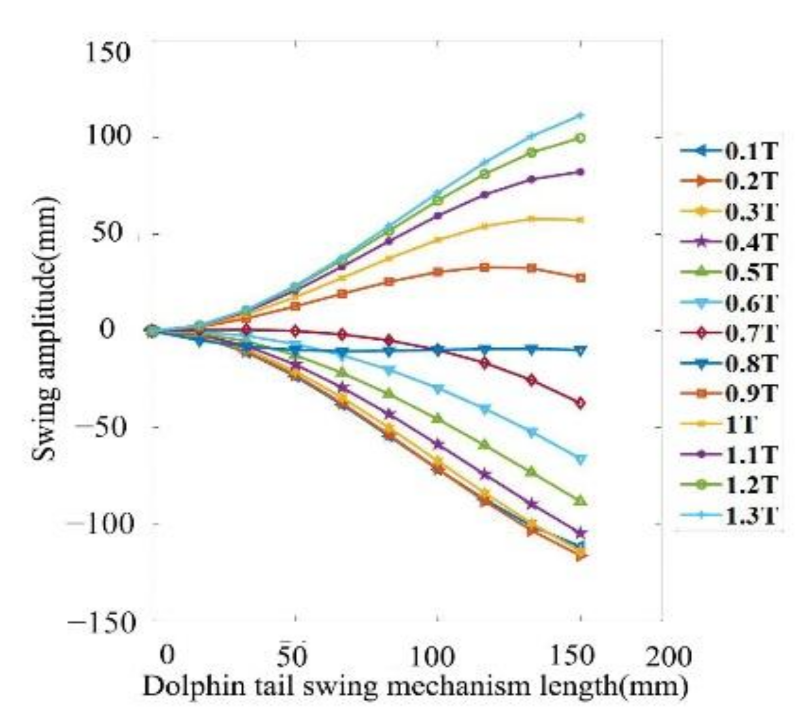
Figure 21.
Matlab software fitting the swing curve of the prototype: (a) 0.1 T prototype swing fitting curve; (b) 0.2 T prototype swing fitting curve; (c) 0.4 T prototype swing fitting curve; (d) 0.8 T prototype swing fitting curve.
Figure 21.
Matlab software fitting the swing curve of the prototype: (a) 0.1 T prototype swing fitting curve; (b) 0.2 T prototype swing fitting curve; (c) 0.4 T prototype swing fitting curve; (d) 0.8 T prototype swing fitting curve.


Figure 22.
Experimental diagram of water tightness of dolphins.

Figure 23.
Motion sequence diagram of bionic dolphin underwater: (a) 0.1 T; (b) 0.3 T; (c) 0.6 T; (d) 0.9 T.
Figure 23.
Motion sequence diagram of bionic dolphin underwater: (a) 0.1 T; (b) 0.3 T; (c) 0.6 T; (d) 0.9 T.

Figure 24.
Swimming speed of experimental prototype of dolphin with different swing amplitude: (a) = 60 mm; (b) = 80 mm; (c) = 100 mm.
Figure 24.
Swimming speed of experimental prototype of dolphin with different swing amplitude: (a) = 60 mm; (b) = 80 mm; (c) = 100 mm.


Table 1.
Bionic robot dolphin servo drive scheme.
| Drive Servo Quantity/Piece | Serial Number | Description |
|---|---|---|
| 1 | 001 | Servo 1 drive |
| 2 | 010 | Servo 2 drive; Servo 1 follow |
| 011 | Servos 1, 2 have phase difference drive | |
| 3 | 100 | Servo 3 drive; Servo 1, 2 follow |
| 101 | Servos 1, 3 have phase difference drive; Servo 2 follow | |
| 110 | Servos 2, 3 have phase difference drive; Servo 1 follow | |
| 111 | Servo 1, 2, 3 have phase difference drive |
Table 2.
Simulation data of No. 111 three joint group.
| Cycle/T | Servo 1 Displacement | Servo 2 Displacement | Servo 3 Displacement |
|---|---|---|---|
| 0.1 | −23.33 | −71.40 | −111.36 |
| 0.2 | −22.69 | −71.32 | −115.98 |
| 0.3 | −20.71 | −67.10 | −113.69 |
| 0.4 | −17.30 | −58.55 | −104.40 |
| 0.5 | −12.45 | −45.57 | −87.96 |
| 0.6 | −6.71 | −29.46 | −65.92 |
| 0.7 | 0.00 | −9.77 | −37.23 |
| 0.8 | −9.77 | −9.77 | −9.77 |
| 0.9 | 12.72 | 30.46 | 27.49 |
| 1 | 17.50 | 47.03 | 57.40 |
| 1.1 | 20.84 | 59.54 | 82.21 |
| 1.2 | 22.69 | 67.36 | 99.76 |
| 1.3 | 23.33 | 71.40 | 111.36 |
Table 3.
No. 111 group nine joint simulation data.
| Cycle/T | Joint 1 | Joint 2 | Joint 3 | Joint 4 | Joint 5 | Joint 6 | Joint 7 | Joint 8 | Joint 9 |
|---|---|---|---|---|---|---|---|---|---|
| 0.1 | −2.92 | −10.89 | −23.33 | −38.00 | −54.18 | −71.40 | −87.03 | −100.62 | −111.36 |
| 0.2 | −2.76 | −10.48 | −22.69 | −37.27 | −53.59 | −71.32 | −87.89 | −102.98 | −115.98 |
| 0.3 | −2.41 | −9.43 | −20.71 | −34.36 | −49.89 | −67.10 | −83.63 | −99.28 | −113.69 |
| 0.4 | −1.85 | −7.69 | −17.30 | −29.16 | −42.91 | −58.55 | −74.05 | −89.37 | −104.40 |
| 0.5 | −1.11 | −5.28 | −12.45 | −21.61 | −32.60 | −45.57 | −59.03 | −73.09 | −87.96 |
| 0.6 | −0.29 | −2.49 | −6.71 | −12.53 | −20.00 | −29.46 | −40.04 | −52.02 | −65.92 |
| 0.7 | 0.59 | 0.70 | 0.00 | −1.75 | −4.83 | −9.77 | −16.45 | −25.33 | −37.23 |
| 0.8 | −4.89 | −8.01 | −9.77 | −10.37 | −10.26 | −9.77 | −9.29 | −9.16 | −9.77 |
| 0.9 | 2.04 | 6.50 | 12.72 | 19.25 | 25.41 | 30.46 | 33.03 | 32.44 | 27.49 |
| 1 | 2.51 | 8.57 | 17.50 | 27.40 | 37.49 | 47.03 | 54.07 | 57.94 | 57.40 |
| 1.1 | 2.79 | 9.97 | 20.84 | 33.24 | 46.37 | 59.54 | 70.41 | 78.35 | 82.21 |
| 1.2 | 2.93 | 10.71 | 22.69 | 36.62 | 51.70 | 67.36 | 81.03 | 92.17 | 99.76 |
| 1.3 | 2.92 | 10.89 | 23.33 | 38.00 | 54.18 | 71.40 | 87.03 | 100.62 | 111.36 |
Table 4.
Simulation parameters of the bionic dolphin.
| Parameter | ||||
|---|---|---|---|---|
| head | 0.8 | 0.172 | 0.018258 | 0.036296 |
| Joint 1 | 0.6 | 0.074 | 0.006576 | 0.011864 |
| Joint 2 | 0.5 | 0.074 | 0.002515 | 0.006076 |
| Joint 3 | 0.4 | 0.074 | 0.00387 | 0.0061 |
| Caudal fin | 0.1 | 0.128 | 0.000372 | 0.00692 |
Table 5.
Dolphin prototype swing coordinate parameters.
| Coordinate | 525 | 550 | 575 | 600 | 625 | 650 | 675 | 700 | 725 | 815 | |
|---|---|---|---|---|---|---|---|---|---|---|---|
| Cycle | |||||||||||
| 0.1 T | 0.2 | 1.6 | 4.4 | 7.0 | 10.6 | 17 | 22 | 32 | 42 | 80 | |
| 0.2 T | 0 | 1.0 | 2.8 | 4.8 | 8 | 12 | 16.2 | 21 | 27 | 60 | |
| 0.4 T | 0 | −0.9 | −2.9 | −5 | −8.3 | −12 | −16 | −22 | −28 | −59 | |
| 0.8 T | −0.2 | −1.8 | −5 | −7.2 | −11.8 | −17.4 | −23.8 | −32.2 | −42.4 | −79 | |
Publisher’s Note: MDPI stays neutral with regard to jurisdictional claims in published maps and institutional affiliations. |
© 2021 by the authors. Licensee MDPI, Basel, Switzerland. This article is an open access article distributed under the terms and conditions of the Creative Commons Attribution (CC BY) license (https://creativecommons.org/licenses/by/4.0/).
Share and Cite
MDPI and ACS Style
Zhang, B.; Li, Q.; Wang, T.; Wang, Z. Development of a Bionic Dolphin Flexible Tail Experimental Device Driven by a Steering Gear. Actuators 2021, 10, 167. https://0-doi-org.brum.beds.ac.uk/10.3390/act10070167
AMA Style
Zhang B, Li Q, Wang T, Wang Z. Development of a Bionic Dolphin Flexible Tail Experimental Device Driven by a Steering Gear. Actuators. 2021; 10(7):167. https://0-doi-org.brum.beds.ac.uk/10.3390/act10070167
Chicago/Turabian StyleZhang, Bo, Qingxiang Li, Tao Wang, and Zhuo Wang. 2021. "Development of a Bionic Dolphin Flexible Tail Experimental Device Driven by a Steering Gear" Actuators 10, no. 7: 167. https://0-doi-org.brum.beds.ac.uk/10.3390/act10070167
Note that from the first issue of 2016, this journal uses article numbers instead of page numbers. See further details here.