Adaptive Super-Twisting Sliding Mode Control of Underwater Mechanical Leg with Extended State Observer

Abstract

Underwater manipulation is one of the most significant functions of the deep-sea crawling and swimming robot (DCSR), which relies on the high-accuracy control of the body posture. As the actuator of body posture control, the position control performance of the underwater mechanical leg (UWML) thus determines the performance of the underwater manipulation. An adaptive super-twisting sliding mode control method based on the extended state observer (ASTSMC-ESO) is proposed to enhance the position control performance of the UWML by taking into account the system’s inherent nonlinear dynamics, uncertainties, and the external disturbances from hydrodynamics, dynamic seal resistance, and compensation oil viscous resistance. This newly designed controller incorporates sliding mode (SMC) feedback control with feedforward compensation of the system uncertainties estimated by the ESO, and the external disturbances of the hydrodynamics by fitting the parameters, the dynamic seal resistance, and the compensation oil viscous resistance to the tested results. Additionally, an adaptive super-twisting algorithm (AST) with integral action is introduced to eliminate the SMC’s chattering phenomenon and reduce the system’s steady-state error. The stability of the proposed controller is proved via the Lyapunov method, and the effectiveness is verified via simulation and comparative experimental studies with SMC and the adaptive fuzzy sliding mode control method (AFSMC).

1. Introduction

With the increasingly continuous consumption of land resources, the pace of human exploration and the development of ocean resources is accelerating and gradually moving from shallow waters to the deep seas. Recently, with the development of robot technology, numerous robots have been increasingly applied in marine engineering. Therefore, deep-sea robots have attracted more and more attention to research. Compared with wheeled robots and tracked robots, legged robots have excellent motion flexibility, strong obstacle avoidance ability, and excellent terrain adaptation [1], making them a hot research topic in recent years [2,3,4]. As a special type of legged robots, the DCSR combines swimming, walking, and underwater manipulating functions, therefore being an important equipment for marine engineering.

Since the robot body is the base of the manipulator equipped on the robot, high-accuracy position control of the UWML is of great significance to improve the robot’s posture control performance, thus enhancing the manipulating performance. Currently, model-based control is the primary method of the high-performance control of dynamic systems, but an accurate model of the control object is required. However, as an inherent nonlinear and strongly coupled dynamic system, the UWML not only has complex nonlinear characteristics but is also influenced by system uncertainties (i.e., parametric uncertainties and unmodeled uncertainties) and external disturbances caused by the deep-sea environment (i.e., hydrodynamic, dynamic seal resistance, and compensation oil viscous resistance). The combined effect of these factors makes it difficult to establish an accurate dynamic model of the UWML, thus exacerbating the difficulty of control.

To overcome nonlinearity and the uncertainties of manipulators, many elegant control techniques [5,6,7,8,9,10,11] were proposed. Among them, the SMC-based methods are the most widely used due to their simple design and robustness against uncertainties and disturbances [12]. However, these methods require an infinite switching control action to handle system uncertainties, which would aggravate the undesired chattering phenomenon. Moreover, the upper bounds of the external disturbances and the system uncertainties must be well known to obtain a stable closed-loop control law. Another issue in SMC-based methods is that of asymptotic convergence, which may not meet the high-performance control of the robotic systems [13].

To restrain chattering, some momentous methods, such as the boundary layer method, the modified switching signal with saturation, etc., have been introduced; however, the presence of the finite steady-state error may cause degradation of the tracking ability [14]. Therefore, high-order sliding mode control (HOSMC) approaches, which provide effective solutions to the chattering problem without sacrificing the control performance, were developed to improve the performance of the classical SMC [15]. In particular, the super-twisting control (STC) has been a widely applied HOSMC since its inception [16].

As a prototype of the HOSMC, STC can effectively suppress the chattering phenomenon since the discontinuous signum function is concealed in the time derivative of the sliding variable [15,17]. However, if the states are far from the sliding surface, the bounded correction terms will result in a very slow convergence of the sliding variable [18]. Moreover, although STC yields a smooth control signal, chattering is still possible. For example, in situations where the upper bound of system uncertainties is difficult to obtain accurately, the largest possible parameters are often selected to ensure the finite-time stability condition, which may result in system oscillation [19]. Therefore, various new STC algorithms have been proposed to enhance the performance of traditional STC. A modified STC was proposed to improve the convergence speed and robustness, in which two linear correction terms were added to the traditional STC to form a double-closed-loop feedback structure [18]. An adaptive STC (ASTC) was synthesized to avoid the problem of difficulty in determining the upper bound of system uncertainties in practical applications, where a double-layer gain-adaptation function was introduced into the traditional STC to determine the two control parameters [20].

In addition, many researchers also conducted a series of observer-based control methods to deal with the uncertainties and disturbances of the dynamic systems, in which observers were applied to estimate the total system uncertainties and disturbances to synthesize a feedforward compensation. Such observers include the disturbance observer (DOB) [21], the sliding mode disturbance observer (SMDO) [22,23], the extended state observer (ESO) [24,25,26,27], etc. An adaptive fuzzy sliding mode control method based on a disturbance observer was proposed to control a manipulator, in which a fuzzy system was adopted to approximate the modeling uncertainties while the disturbances were estimated via a DOB online, respectively, and both were then compensated in SMC [21]. Due to the advantages of estimating the system’s states and uncertainties simultaneously with little model information and a simple design process, ESO was widely applied in the control of manipulators. An adaptive extended state observer (ESO) is developed to estimate the unmeasured states and eliminate the impact of the unknown disturbances and parameter uncertainties for the control of an aircraft skin inspection robot [26]. To deal with the time-varying output constraints and external disturbances of a manipulator, an ESO was applied to estimate the unmeasurable states and total disturbances, which were then incorporated into the controller design [25].

Based on the above analysis and the UWML’s system characteristics, by borrowing ideas from ESO and AST and integrating them via an SMC control action, a novel adaptive super-twisting sliding mode control method based on the extended state observer (ASTSMC-ESO) is proposed for the high-accuracy position control of the UWML. The introduction of AST can effectively suppress the chattering effect and enhance the steady-state control accuracy while ensuring the robustness of the feedback controller SMC. The integration of ESO and the experimentally tested data can make a feedforward compensation for the system uncertainties, and the external disturbances of the hydrodynamic force, dynamic seal resistance, and compensation oil viscous resistance.

The rest of this paper is organized as follows. Section 2 establishes the models of the UWML and gives the problem formulation. Section 3 presents the ESO design procedure, while Section 4 carries out the ASTSMC-ESO design procedure. Section 5 and Section 6 describe the simulation and experimental verification results, respectively, and some conclusions are made in Section 7.

2. Models and Problem Formulation

2.1. Kinematic Model

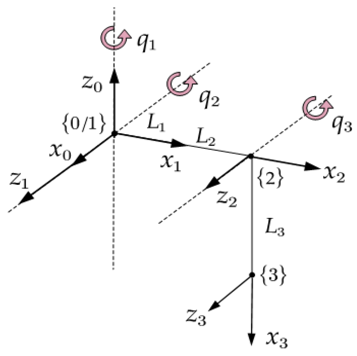
The UWML is a 3-DOF serial mechanism shown in Figure 1. The D-H coordinate systems and the corresponding parameters used to develop the kinematic model of the UWML are shown in Figure 2 and

Table 1. D-H parameters of the UWML.

#	q	d	a	α
0–1	q1	0	L1 (0 m)	90°
1–2	q2	0	L2 (0.66 m)	0°
2–3	q3	0	L3 (0.85 m)	0°

, respectively.

The coordinates of the foot tip of the UWML with respect to the base frame {0} can be determined as:

$${}_{ }{}^{0}p{}_3=\left[\begin{array}{c}x\\ y\\ z\end{array}\right]=\left[\begin{array}{c}-s_1\left(L_1+L_2{c}_2+L_3{s}_{23}\right)\\ c_1\left(L_1+L_2{c}_2+L_3{s}_{23}\right)\\ L_2{s}_2-L_3{c}_{23}\end{array}\right]$$

(1)

Then, the joint angles can be derived using the inverse kinematics, as follows:

$$\{\begin{array}{l}{q}_1=\arctan 2\left(-x, y\right)\\ q_2=\arccos \left(\frac{-z}{\sqrt{M^2+N^2}}\right)-\phi \\ q_3=\arcsin \left(\frac{A^2+z^2-L_2^2-L_3^2}{2L_2{L}_3}\right)\end{array}$$

(2)

where x, y, and z are the coordinates of the foot tip, $s_i=\sin \left(q_i\right)$, $c_i=\cos \left(q_i\right)$, $s_{ij}=\sin \left(q_i+q_j\right)$, $c_{ij}=\cos \left(q_i+q_j\right),A=y/c_1-L_1, M=L_2+L_3{s}_3=\rho \sin \left(\phi \right)$, $N=L_3{c}_3=\rho \cos \left(\phi \right)$, and $\phi =\arctan 2\left(M, N\right)$.

2.2. Dynamic Model

When taking into account the external disturbances of hydrodynamics ${\tau }_w$, dynamic seal resistance ${\tau }_f$, compensation oil viscous resistance ${\tau }_s$, and the system uncertainty d, the dynamic model of the UWML is:

$$\tau =M\ddot{q}+C\dot{q}+G+{\tau }_f+{\tau }_s-{\tau }_w+d$$

(3)

where $\dot{q}$ and $\ddot{q}$ are the joint velocity and acceleration, respectively. M, C, and G are the inertia matrix, the coriolis/centrifugal matrix, and the gravity vector, respectively.

In general, due to parameter perturbation, testing errors, and unmodeled dynamics, the model (3) differs from the actual model of the UWML, and the differences become uncertainties of the system. When considering the impact of system uncertainties, the system parameters M, C, and G and the external disturbances ${\tau }_w$, ${\tau }_f$, and ${\tau }_s$ can be represented as:

$$\{\begin{array}{c}M=M_n+\Delta M\\ C=C_n+\Delta C\\ G=G_n+\Delta G\\ {\tau }_f={\tau }_{fn}+\Delta {\tau }_f\\ {\tau }_s={\tau }_{sn}+\Delta {\tau }_s\\ {\tau }_w={\tau }_{wn}+\Delta {\tau }_w\end{array}$$

(4)

where $M_n$, $C_n$ and $G_n$ are the nominal values of the inertia matrix, the coriolis/centrifugal matrix, and the gravity vector of the UWML, respectively, which can be found in the author’s published article [28]. $\Delta M$, $\Delta C,$ and $\Delta G$ are the modeling uncertainties. ${\tau }_{fn}$ and ${\tau }_{sn}$ are the tested results of the dynamic seal resistance and compensation oil viscous resistance, respectively, which are shown in Figure 3 and Figure 4; ${\tau }_{wn}$ is the hydrodynamics calculated with the fitted parameters, of which the detailed analysis can be found in the author’s recently published article [29]. $\Delta {\tau }_f$, $\Delta {\tau }_s$, and $\Delta {\tau }_w$ represent the uncertainties caused by the testing errors.

Substituting (4) into (3) yields the nonlinear dynamic model of the UWML:

$$\tau =M_n\ddot{q}+C_n\dot{q}+G_n+{\tau }_{fn}+{\tau }_{sn}-{\tau }_{wn}+\Delta$$

(5)

where $\Delta =\Delta M\ddot{q}+\Delta C\dot{q}+\Delta G+\Delta {\tau }_f+\Delta {\tau }_s-\Delta {\tau }_w+d$ represents the total dynamic uncertainties caused by the parameter uncertainties, testing errors, and unmodeled dynamics. According to the robotic theory, the inertia matrix $M_n$ is a bounded symmetric positive definite matrix, and $M_n-2C_n$ is a skew-symmetric matrix, satisfying $x^T\left(M_n-2C_n\right)x=0$ for any vector x.

To simplify the design and analysis, define the state variable of the UWML as $x={\left[x_1, x_2\right]}^T={\left[q, \dot{q}\right]}^T$, then the dynamic model (5) can be rewritten in a state-space form:

$$\{\begin{array}{l}{\dot{x}}_1=x_2 \\ {\dot{x}}_2=M_n^{-1}\tau -M_n^{-1}\left(C_n{x}_2+G_n+{\tau }_{fn}+{\tau }_{sn}-{\tau }_{wn}\right)-M_n^{-1}\Delta \end{array}$$

(6)

2.3. Control Objective

The control objective is to design a high-performance controller for the UWML with strong nonlinearities (i.e., structure nonlinearity, friction resistance, and oil resistance nonlinearity) and uncertainties (i.e., parameter uncertainties, unmodeled dynamics) to ensure the actual foot trajectory $y\left(t\right)$ tracking the planned trajectory $y_d\left(t\right)$ as close as possible.

3. Observer Design

To reduce the impact of uncertainties on the UWML’s control performance, the total uncertainties of the dynamic system (6) have to be compensated in the controller, which can be extended to a new state variable and estimated via an ESO. Based on this idea, the uncertainties $-M_n^{-1}\Delta$ is extended to a state variable $x_3$, and its time derivative is set to be $h\left(t\right)$. Thus, the extended dynamic model of the UWML can be expressed as:

$$\{\begin{array}{l}{\dot{x}}_1=x_2\hfill \\ {\dot{x}}_2=M_n^{-1}\tau -M_n^{-1}\left(C_n{x}_2+G_n+{\tau }_{fn}+{\tau }_{sn}-{\tau }_{wn}\right)+x_3\hfill \\ {\dot{x}}_3=h\left(t\right)\hfill \end{array}$$

(7)

Assumption 1.

$h\left(t\right)$ is bounded, and there exists a constant $h_0>0$ such that $\Vert h\left(t\right)\Vert \le h_0$.

Based on the extended system model (7), the ESO can be designed as:

$$\{\begin{array}{l}{\dot{\hat{x}}}_1={\hat{x}}_2+l_1{\omega }_0\left(x_1-{\hat{x}}_1\right)\hfill \\ {\dot{\hat{x}}}_2=M_n^{-1}\tau -M_n^{-1}(C_n{x}_2+G_n+{\tau }_{fn}+{\tau }_{sn}-{\tau }_{wn})+{\hat{x}}_3+l_2{\omega }_0^2\left(x_1-{\hat{x}}_1\right)\hfill \\ {\dot{\hat{x}}}_3=l_3{\omega }_0^3\left(x_1-{\hat{x}}_1\right)\hfill \end{array}$$

(8)

where $\widehat{x}={\left[{\widehat{x}}_1, {\widehat{x}}_2, {\widehat{x}}_3\right]}^T$ is the estimated state, $L={\left[l_1, l_2, l_3\right]}^T$ is the observer gain, and ${\omega }_0>0$ is the observer bandwidth.

To ensure the stability of ESO, the observer gain is designed to satisfy the following polynomial:

$$p\left(s\right)=s^3+l_1{s}^2+l_{2}s+l_3={\left(s+1\right)}^3$$

(9)

Let $\tilde{x}=x-\widehat{x}={\left[{\tilde{x}}_1, {\tilde{x}}_2, {\tilde{x}}_3\right]}^T$ denote the observation error, then the dynamic of the observation error can be obtained from (7) and (8):

$$\{\begin{array}{l}{\dot{\tilde{x}}}_1={\tilde{x}}_2-l_1{\omega }_0{\tilde{x}}_1\hfill \\ {\dot{\tilde{x}}}_2={\tilde{x}}_3-l_2{\omega }_0^2{\tilde{x}}_1\hfill \\ {\dot{\tilde{x}}}_3=h\left(t\right)-l_3{\omega }_0^3{\tilde{x}}_1\hfill \end{array}$$

(10)

Define the proportional observation error ${\epsilon }_i={\tilde{x}}_i/{\omega }_0^{i-1}$, $i=1, 2, 3$. Then, the dynamic of the proportional observation error can be obtained according to (10):

$$\dot{\epsilon }={\omega }_{0}A\epsilon +B\frac{h\left(t\right)}{{\omega }_0^2}$$

(11)

where $\epsilon ={\left[{\epsilon }_1, {\epsilon }_2, {\epsilon }_3\right]}^T, A=\left[\begin{array}{ccc}-3I_{3\times 3}& I_{3\times 3}& 0_{3\times 3}\\ -3I_{3\times 3}& 0_{3\times 3}& I_{3\times 3}\\ -I_{3\times 3}& 0_{3\times 3}& 0_{3\times 3}\end{array}\right], B=\left[\begin{array}{c}{0}_3\\ 0_3\\ I_3\end{array}\right]$; $0_{3\times 3}$ and $I_{3\times 3}$ are the 3×3 zero matrix and the identity matrix, respectively; and $0_3$ and $I_3$ are the 3-dimensional zero vector and the unit vector, respectively.

Theorem 1 

[27,30]. Under Assumption 1, according to the dynamic Equation (6), when designing an ESO (8), there exist constants ${\sigma }_{ij}>0$, $c>0$, and finite time $T_1>0$, such that the state estimation error ${\tilde{x}}_{ij}$ is bounded, and its value of the state estimation error can be adjusted by changing the bandwidth ${\omega }_0$: 

$$\left|{\tilde{x}}_{ij}\right|\le {\sigma }_{ij} , {\sigma }_{ij}=O\left(\frac{1}{{\omega }_0^c}\right); i=j=1, 2, 3 \forall t\ge T_1$$

(12)

4. Controller Design

4.1. Design of SMC-ESO Controller

Since the UWML is subject to strong external disturbances and uncertainties when working in a complex underwater environment, an SMC-ESO control method, possessing strong robustness, is adopted to deal with the trajectory tracking problem of the UWML intuitively.

The tracking errors of the joint position and velocity of the UWML are defined as $e_1$ and $e_2$, respectively:

$$e_1=x_{1d}-x_1$$

(13)

$$e_2={\dot{x}}_{1d}-x_2$$

(14)

where $x_{1d}$ and ${\dot{x}}_{1d}$ are the joint position and velocity command obtained from the reference foot trajectory via inverse kinematics (6).

Then, the sliding mode surface function $s$ can be defined as:

$$s=e_2+{\lambda }_1{e}_1$$

(15)

where ${\lambda }_1\in R^{3\times 3}$ is a positive definite diagonal parameter matrix.

Based on Equations (7) and (13)–(15), the time derivative of $s$ can be expressed as:

$$\begin{array}{ll}\dot{s}& ={\dot{e}}_2+{\lambda }_1{\dot{e}}_1\\ & \begin{array}{c}={\ddot{x}}_{1d}+{\lambda }_1{e}_2-M_n^{-1}\tau +M_n^{-1}\left(C_n{x}_2+G_n+{\tau }_{fn}+{\tau }_{sn}-{\tau }_{wn}\right)-x_3\end{array}\end{array}$$

(16)

From (16), the SMC-ESO with an exponential convergence rate can be designed as:

$$\tau ={\tau }_{eq}+{\tau }_{sw}$$

(17)

$${\tau }_{eq}=M_n\left({\ddot{x}}_{1d}+{\lambda }_1{e}_2\right)-M_n{\widehat{x}}_3+C_n{x}_2+G_n+{\tau }_{fn}+{\tau }_{sn}-{\tau }_{wn}$$

(18)

$${\tau }_{sw}=M_n\left({\lambda }_{1}s+{\lambda }_r\mathrm{sign}\left(s\right)\right)$$

(19)

where $-M_n{\widehat{x}}_3$ is the estimated value of the system uncertainties $\Delta$, which can be calculated from the extended state of the ESO; ${\lambda }_2$ and ${\lambda }_r\in R^{3\times 3}$ are positive definite diagonal parameter matrices; and $\mathrm{sign}\left(s\right)$ is the signum function vector.

Although the above SMC-ESO can ensure the stability of the closed-loop system, it has inherent defects of conventional SMC. On the one hand, the sliding mode switching control action ${\tau }_{sw}$ contains a discontinuous signum function $\mathrm{sign}\left(s\right)$ leading to the “chattering” phenomenon. On the other hand, the gain ${\lambda }_r$ of ${\tau }_{sw}$ must be selected based on the upper bound of the system uncertainties, which are usually unknown. If the value is too conservative to be large, it will exacerbate the system chattering. However, if a smaller value is selected, it may cause the system to be unstable. To avoid sacrificing the control accuracy or robustness by using traditional methods such as the boundary layer method and the modified switching signal with saturation to suppress chattering, this paper introduces the AST into the above SMC-ESO to eliminate the chattering and improve the control performance of the system.

4.2. Design of ASTSMC-ESO Controller

To eliminate the chattering effect of the conventional SMC, an ASTSMC-ESO is proposed, in which a super-twisting control action [16,31] is applied to replace the discontinuous sliding mode control law ${\tau }_{sw}$:

$$\{\begin{array}{l}{\tau }_{sw}=M_n\left[\alpha \left(t\right){\left|s\right|}^{\frac{1}{2}}\mathrm{sign}\left(s\right)+k_1\left(t\right)s-\xi +\varphi \left(s, L\left(t\right)\right)\right]\\ \dot{\xi }=-\beta \left(t\right)sign\left(s\right)-k_2\left(t\right)s \end{array}$$

(20)

where $\xi$ is an intermediate variable; $L\left(t\right)$ is the parameter adaptive function to be designed later; and $\alpha \left(t\right)$, β(t), $k_1\left(t\right),$ and $k_2\left(t\right)$ are positive definite parameter matrices; $\varphi \left(s, L\left(t\right)\right)=-\dot{L}\left(t\right)s/L\left(t\right)$.

In the above super-twisting algorithm, the values of $\alpha \left(t\right)$ and $\beta \left(t\right)$ should be determined based on the upper bound of system uncertainties and its rate of change. For the UWML, since the system uncertainties have been estimated via the expanded state observer, α(t) and β(t) should be determined based on the upper bound of the estimation error and its rate of change. Since these two values are both difficult to determine, the adaptive laws are designed for the parameters of (20), which are shown in (21):

$$\{\begin{array}{c}\alpha \left(t\right)=\sqrt{L\left(t\right)}{\alpha }_0\\ \beta \left(t\right)=L\left(t\right){\beta }_0\\ k_1\left(t\right)=L\left(t\right)k_{10}\\ k_2\left(t\right)=L^2\left(t\right)k_{20}\end{array}$$

(21)

where ${\alpha }_0$, ${\beta }_0$, $k_{10}$, and $k_{20}$ are the constants, and $L\left(t\right)$ are adaptive functions that will be designed using a double-layer gain-adaptation algorithm in Section 4.4.

Substituting (17)–(20) into (16) yields:

$$\dot{s}=-{\tilde{x}}_3-\alpha {\left|s\right|}^{\frac{1}{2}}\mathrm{sign}\left(s\right)-k_{1}s-{\int }_0^t\left(\beta \mathrm{sign}\left(s\right)+k_{2}s\right)dt-\varphi \left(s, L\right)$$

(22)

Define $z=-{{\int }^{ }}_0^t\left(\beta \mathrm{sign}\left(s\right)+k_{2}s\right)dt-{\tilde{x}}_3$, $f\left(t\right)=-{\dot{\tilde{x}}}_3$, then (22) can be rewritten as:

$$\{\begin{array}{l}\dot{s}=-\alpha {\left|s\right|}^{\frac{1}{2}}sign\left(s\right)-k_{1}s+z-\varphi \left(s, L\right)\\ \dot{z}=-\beta sign\left(s\right)-k_{2}s+f\left(t\right) \end{array}$$

(23)

According to Theorem 1 and Equation (10), it can be seen that $f\left(t\right)=-{\dot{\tilde{x}}}_3=-h\left(t\right)+l_3{\omega }_0^3{\tilde{x}}_1$ is bounded. Let its upper bound be denoted as ${\sigma }_0$, thus $\Vert f\left(t\right)\Vert \le {\sigma }_0$.

4.3. Controller Stability Analysis

The stability proof of the ASTSMC-ESO is relatively complex. Here, only the following stability theorem is presented. The detailed proof process can be found in Appendix A.

Theorem 2.

Based on Assumption 1, Lemma 1, and Theorem 1, the ASTSMC-ESO controller (17), (18), (20), and the parameter adaptive function (21) are designed for the dynamic system (7) of the UWML. When $L_i\left(t\right)>{\sigma }_{0i}\ge \left|f_i\left(t\right)\right|$, and the appropriate parameters ${\alpha }_{0i}$, ${\beta }_{0i}$, $k_{10i}$ and $k_{20i}$ are selected to make the matrix $P_i$, $B_i$, and $Q_i$ (which was expressed as (24)–(26)) positive definite, then the closed-loop system of the UWML is stable, and the joint position error $e_{1i}$ will converge to the origin in finite time, where $i=1, 2, 3$.

$$P_i=\frac{1}{2}\left[\begin{array}{ccc}4{\beta }_{0i}+{\alpha }_{0i}^2& {\alpha }_{0i}{k}_{10i}& -{\alpha }_{0i}\\ {\alpha }_{0i}{k}_{10i}& 2k_{20i}+k_{10i}^2& -k_{10i}\\ -{\alpha }_0& -k_{10i}& 2\end{array}\right]$$

(24)

$$B_i=k_{10i}\left[\begin{array}{ccc}{\beta }_{0i}+2{\alpha }_{0i}^2& 0& 0\\ 0& k_{20i}+k_{10i}^2& -k_{10i}\\ 0& -k_{10i}& 1\end{array}\right]$$

(25)

$$Q_i=A_i-C_i$$

(26)

$$A_i=\frac{{\alpha }_{0i}}{2}\left[\begin{array}{ccc}2{\beta }_{0i}+{\alpha }_{0i}^2& 0& -{\alpha }_{0i}\\ 0& 2k_{20i}+5k_{10i}^2& -3k_{10i}\\ -{\alpha }_{0i}& -3k_{10i}& 1\end{array}\right]$$

(27)

$$C_i=\left[\begin{array}{ccc}-{\alpha }_{0i}{\vartheta }_i& -\frac{1}{2}{k}_{10i}{\vartheta }_i& {\vartheta }_i\\ -\frac{1}{2}{k}_{10i}{\vartheta }_i& 0& 0\\ {\vartheta }_i& 0& 0\end{array}\right]$$

(28)

$${\vartheta }_i=\frac{f_i\left(t\right)sign\left(s_i\right)}{L_i\left(t\right)}$$

(29)

Compared to the conventional ASTSMC-ESO algorithm applied in other fields [32], The main improvement of the method proposed in this paper is to increase the convergence speed of the system states. It can be seen from the proof results (A16) of the ASTSMC-ESO in this paper, when the Lyapunov function V is relatively close to the equilibrium, the nonlinear term ${\lambda }_2{V}_i^{1/2}$ is much bigger than the linear term ${\lambda }_1{V}_i$, so the nonlinear term ${\lambda }_2{V}_i^{1/2}$ mainly determines the convergence speed. When the Lyapunov function V is far from the equilibrium, the linear term ${\lambda }_1{V}_i$ is much bigger than the nonlinear term ${\lambda }_2{V}_i^{1/2}$, so the linear term ${\lambda }_1{V}_i$ mainly determines the convergence speed. Nevertheless, for conventional ASTSMC-ESO, no matter where the Lyapunov function is, the convergence speed is determined only by the nonlinear term ${\lambda }_2{V}_i^{1/2}$, so when the Lyapunov function V is far from the equilibrium, slow convergence speed will present [20]. The above analysis shows that by adding linear terms to the conventional AST, the ASTSMC-ESO designed in this paper improves the convergence characteristics. From the viewpoint of the controller, the newly designed ASTSMC-ESO is equivalent to adding a proportional and integral sliding mode control action than the conventional one. Therefore, the convergence speed and control accuracy are improved.

4.4. Design of the Adaptive Function $L_i\left(t\right)$

As mentioned in the previous design process, the parameters ${\alpha }_i\left(t\right)$, ${\beta }_i\left(t\right)$, $k_{1i}\left(t\right),$ and $k_{2i}\left(t\right)$ of (20) must be adjusted via the adaptive function $L_i\left(t\right)$. To ensure stability, $L_i\left(t\right)$ should satisfy the condition $L_i\left(t\right)>\left|f_i\left(t\right)\right|$, where a dual-layer adaption algorithm is adopted to design $L_i\left(t\right)$.

According to the concept of “equivalent control”, the system (23) enters the sliding mode surface when $s_i={\dot{s}}_i=0$ and $z_i={\dot{z}}_i=0$. To maintain the system trajectory on the sliding surface, the equivalent effect of the discontinuous switching term ${\beta }_i\mathrm{sign}\left(s_i\right)$, denoted as $u_{eqi}$, can be used to compensate for $f_i\left(t\right)$:

$$u_{eqi}={\beta }_i\mathrm{sign}\left(s_i\right){|}_{eq}=f_i\left(t\right)$$

(30)

In practical applications, $u_{eqi}$ can be estimated from ${\beta }_i\mathrm{sign}\left(s_i\right)$ online via a low-pass filter:

$${\dot{u}}_{eqi}=\frac{1}{\tau }\left({\beta }_i\mathrm{sign}\left(s_i\right)-u_{eqi}\right)$$

(31)

where $\tau$ is the time constant of the filter.

From (30) and (31), an online estimation of $f_i\left(t\right)$ can be achieved by filtering the discontinuous switch term. This estimation value can be used to design $L_i\left(t\right)$:

$$L_i\left(t\right)=l_{0i}+l_i\left(t\right)$$

(32)

where $l_{0i}$ is a small positive design parameter, $l_i\left(t\right)$ is a time-varying parameter whose rate of change is defined as the first-layer adaptive algorithm:

$${\dot{l}}_i\left(t\right)=-\left({\rho }_{0i}+{\rho }_i\left(t\right)\right)\mathrm{sign}\left({\delta }_i\right)$$

(33)

where ${\rho }_{0i}$ is a constant positive parameter, ${\rho }_i\left(t\right)$ is a time-varying parameter, and its rate of change is defined as the second-layer adaptive algorithm:

$${\dot{\rho }}_i\left(t\right)={\gamma }_i\left|{\delta }_i\right|$$

(34)

where ${\gamma }_i$ is a positive design parameter.

The variable ${\delta }_i$ in the above two-layer adaptive rate is:

$${\delta }_i=L_i\left(t\right)-\frac{1}{a_i{\beta }_{0i}}\left|u_{eqi}\right|-{ϵ}_i$$

(35)

where $0<a_i<1/{\beta }_{0i}<1$, and ${ϵ}_i$ is a small positive parameter.

Using the above dual-layer adaption algorithm, the condition $L_i\left(t\right)>\left|f_i\left(t\right)\right|$ can be guaranteed within a finite time, which can be described as the following theorem.

Theorem 3

[20]. Consider the system in (23) is subject to uncertainty $f\left(t\right),$ which satisfies the two constraints $\left|f_i\left(t\right)\right|<{\sigma }_{0i}$ and $\left| {\dot{f}}_i\left(t\right)\right|<{\sigma }_{1i}$, where the positive scalars $a_0$ and $a_1$ are finite but unknown. Then, the dual-layer adaption algorithm in (32)–(34) ensures $L_i\left(t\right)>\left|f_i\left(t\right)\right|$ in finite time.

Theorem 3 is a supplement to Theorem 2, which resolves the parameter selecting-problem of the ASTSMC-ESO. In practical applications, in order to reduce the influence of noise and disturbances, ${\dot{\rho }}_i\left(t\right)$ can be obtained with a dead zone ${\delta }_{i0}$:

$${\dot{\rho }}_i\left(t\right)=\{\begin{array}{c}\begin{array}{cc}{\gamma }_i\left|{\delta }_i\right|, & \mathrm{if} \left|{\delta }_i\right|>{\delta }_{i0}\end{array}\\ \begin{array}{cc} 0, & \mathrm{otherwise} \end{array}\end{array}$$

(36)

From Equations (17), (18), (20), and (21), it can be seen that the ASTSMC-ESO mainly consists of two parts: ${\tau }_{eq}$ is the model compensation term, which enables the system output to quickly track the desired trajectory, while ${\tau }_{sw}$ is the stabilizing feedback term, which ensures that the tracking error of the system is stable. Further analysis of the composition of ${\tau }_{sw}$ reveals that, in addition to the conventional approaching term ${\left|s\right|}^{\frac{1}{2}}\mathrm{sign}\left(s\right)$ and the exponential approaching term $k_{1}s$, it also includes an integral term of the signum function of the sliding mode variable ${{\int }^{ }}_0^t\beta \mathrm{sign}\left(s\right)dt$ and an integral term of the sliding mode variable itself ${{\int }^{ }}_0^t{k}_{2}sdt$. The former compensates for the estimation error of the system uncertainties, while the latter reduces the steady-state error of the system, thereby improving both the dynamic convergence speed and the steady-state control accuracy of the system. In addition, an adaptive function $L_i\left(t\right)$ is designed to adjust the parameters ${\alpha }_i\left(t\right)$, ${\beta }_i\left(t\right)$, $k_{1i}\left(t\right),$ and $k_{2i}\left(t\right)$ of the controller, which effectively eliminates the chattering phenomenon of the SMC. The principle of the ASTSMC-ESO control system for the UWML is shown in Figure 5.

5. Simulation Results

To verify the effectiveness of the proposed ASTSMC-ESO, the trajectory tracking performance of the UWML is studied via simulation.

5.1. Simulation Model

The simulation model of the UWML is shown in Figure 6, which is built using Simulink/Simscape. The parameters of the UWML are listed in

Table 2. Parameters of the UWML.

Link	Mass (kg)	Center of Mass (m)	Inertia Matrix (kg·m2)
1	10.758	[0, 0.001, −0.017]T	diag{0.044, 0.039, 0.032}
2	19.261	[−0.154, 0, −0.014]T	diag{0.135, 1.455, 1.375}
3	10.375	[−0.391, 0, −0.045]T	diag{0.138, 2.437, 2.327}

. To simulate the effects of the dynamic seal resistance ${\tau }_f$, compensation oil viscous resistance ${\tau }_s$, and the hydrodynamic ${\tau }_w$, a tabular form of ${\tau }_s$ and ${\tau }_w$ from the tested results in Figure 3 and Figure 4, which are added to the dynamic model of the UWML, while ${\tau }_w$ is added according to the calculation formulas with the fitted hydrodynamic parameters. The initial values of the system states are $x_1={\left[0.294, 0.158,-0.105\right]}^{\mathrm{T}}$, and $x_2={\left[0, 0, 0\right]}^{\mathrm{T}}$; the initial values of the states of ESO are ${\widehat{x}}_1={\left[0, 0, 0\right]}^{\mathrm{T}}$, ${\widehat{x}}_2={\left[0, 0, 0\right]}^{\mathrm{T}}$, and ${\widehat{x}}_3={\left[0, 0, 0\right]}^{\mathrm{T}}$, while the bandwidth is ${\omega }_0=60$. The controller parameters are presented in

Table 3. Parameters of the simulation controller.

Controller

Parameters

ASTSMC-ESO

${\lambda }_1=\mathrm{diag}\left\{400, 800, 800\right\}, k_{10}=\mathrm{diag}\left\{12, 20, 4\right\}, k_{20}=\mathrm{diag}\left\{200, 200, 200\right\}$, ${\alpha }_0=\mathrm{diag}\left\{6.32, 6.32, 8.94\right\}, {\beta }_0=\mathrm{diag}\left\{5, 5, 10\right\}, \tau =\mathrm{diag}\left\{0.01, 0.01, 0.01\right\}$, $a=\mathrm{diag}\left\{0.86, 0.86, 0.86\right\}, l_0=\mathrm{diag}\left\{0.5, 0.5, 0.5\right\}, {\rho }_0=\mathrm{diag}\left\{0.5, 0.5, 0.5\right\}$, $\gamma =\mathrm{diag}\left\{0.002, 0.002, 0.002\right\}, {\delta }_0=\mathrm{diag}\left\{50, 50, 50\right\}$, $ϵ=\mathrm{diag}\left\{0.1, 0.1, 0.1\right\}$

. For convenience, a cycloidal foot trajectory [28] is planned for the UWML, which is shown in (37), with the step length $S_0=0.4 \mathrm{m}$, step height $H_0=0.2 \mathrm{m}$, step period $T=8 \mathrm{s}$, translational phase period $T_m=4 \mathrm{s}$, and initial height of the foot tip $z_0=-0.61$.

$$\{\begin{array}{c}x=\left\{\begin{array}{c}\frac{S_0}{2\pi }\left(\frac{2\pi t}{T_m}-sin\left(\frac{2\pi t}{T_m}\right)\right)-\frac{S_0}{2},\left(0\le t\le T_m\right)\hfill \\ S_0-\frac{S_0}{2\pi }\left(\frac{2\pi t}{T_m}-sin\left(\frac{2\pi t}{T_m}\right)\right)-\frac{S_0}{2},\left(T_m<t\le \mathrm{T}\right)\hfill \end{array}\right.\hfill \\ y=L_2,\left(0\le t\le T_m\right)\hfill \\ z=\left\{\begin{array}{c}2H_0\left(\frac{t}{T_m}-\frac{1}{4\pi }sin\left(\frac{4\pi t}{T_m}\right)\right)+z_0,\left(0\le t\le T_m/2\right)\hfill \\ -2H_0\left(\frac{t}{T_m}-\frac{1}{4\pi }sin\left(\frac{4\pi t}{T_m}\right)\right)+2H_0+z_0,\left(T_m/2<t\le T_m\right)\hfill \\ z_0,\left(T_m\le t\le T\right)\hfill \end{array}\right.\hfill \end{array}$$

(37)

5.2. Simulation Study

Three working conditions were studied with the ASTSMC-ESO. Condition 1 is the basic condition, where no disturbances are added to the UWML, and the action time is $0 \mathrm{s}\le t\le 20 \mathrm{s}$, $40 \mathrm{s}\le t\le 60 \mathrm{s}$, and $80 \mathrm{s}\le t\le 100 \mathrm{s}$, respectively. Condition 2 is the condition where the modeling uncertainty disturbances are added, of which the parameters $M$, $C,$ and $G$ of the UWML are set with an amplitude of 50% variation during the time period of $20 \mathrm{s}\le t\le 40 \mathrm{s}$, and the changing law is shown in Equation (38). Condition 3 is the condition where the external disturbances are added, of which the system uncertainty d in the dynamic equation of the UWML has a fluctuation of 50 Nm during the time period of $60 \mathrm{s}\le t\le 80 \mathrm{s}$, and the variation law is shown in Equation (39). The simulation results are shown in Figure 7, Figure 8, Figure 9 and Figure 10.

$$\{\begin{array}{c}M=M_n\left[1+0.5\sin \left(0.25\pi t\right)\right]\left(20\le t\le 40\right)\\ C=C_n\left[1+0.5\sin \left(0.25\pi t\right)\right]\left(20\le t\le 40\right)\\ \begin{array}{c}G=G_n\left[1+0.5\sin \left(0.25\pi t\right)\right]\left(20\le t\le 40\right)\end{array}\end{array}$$

(38)

$$d=50\sin \left(0.25\pi t\right)\left(60\le t\le 80\right)$$

(39)

From the foot trajectory tracking results in Figure 7, it can be seen that the ASTSMC-ESO can accurately control the UWML to move along the planned trajectory under all the three working conditions with tracking errors within 10⁻² mm in all three directions of the workspace, which illustrates the effectiveness of the ASTSMC-ESO. In addition, from Figure 7, we can also see that the foot trajectory tracking errors under two external disturbances are not significantly different from those without disturbances, indicating that the ASTSMC-ESO has excellent robustness. Further analysis of the joint position control results in Figure 8 shows that the actual joint position almost coincides with the reference joint position. Even under the time-varying modeling uncertainties with an amplitude up to 50% of the nominal value of the system parameters in working condition 2 and the external disturbances with an amplitude up to 50 Nm in working condition 3, the position tracking error of each joint can still be maintained within 10⁻⁵ rad and is hardly affected by external disturbances.

The estimated uncertainties in Figure 9 show that no matter which working conditions, the ESO can accurately estimate the system uncertainties. This indicates that the ESO has good estimation ability for the system uncertainties. As can be seen, with the help of the ESO, the uncertainties of different working conditions can be effectively compensated via ASTSMC-ESO, so that the joint control torque can respond quickly and accurately to reduce the impact of these uncertainties on the system performance. In addition, it can be seen from Figure 10 that the parameter’s adaptive function $L_i\left(t\right)$ has good convergence performance and can be adjusted online periodically according to the motion of UWML, thereby eliminating the chattering of SMC.

6. Comparative Experimental Results

To further test the performance of the ASTSMC-ESO, experimental research was conducted with the UWML, of which the test platform is presented in Figure 11, and its main components are listed in

Table 4. The main components of the experimental platform of the UWML.

Name	Specification	Name	Specification
Motor for joint 1/2/3	Kollmorgen TBMS-7646-A	Velocity sensor of joint 2	Tamagawa S2620N271E14
Reducer for joint 1/2/3	Benrun BHS32-160	Position sensor of joint 3	Tamagawa S2640N321E64
Motor driver for joint 1/2/3	Elmo G-SOLTWI15/100ER1	Velocity sensor of joint 3	Tamagawa S2620N271E14
Position sensor of joint 1	Tamagawa TS2660N31E148	Motion controller	Beckhoff CX5140 PLC
Velocity sensor of joint 1	Tamagawa TS2620N271E14	Main power	DC48V
Position sensor of joint 2	Tamagawa TS2620N271E14	Control power	DC24V

. To illustrate the control performance, comparative studies were carried out on the ASTSMC-ESO, SMC [33], and AFSMC [34].

6.1. Comparison Controllers

(1) SMC: This is the traditional sliding mode controller with the compensation of external disturbances of ${\tau }_f$, ${\tau }_s,$ and ${\tau }_w$:

$$\tau =M_n\left({\ddot{x}}_{1d}+{\lambda }_1{e}_2\right)+C_n{x}_2+G_n+{\tau }_{fn}+{\tau }_{sn}-{\tau }_{wn}+{\lambda }_{2}s+{\lambda }_r\mathrm{sign}\left(s\right)$$

(40)

where ${\lambda }_1$, ${\lambda }_2,$ and ${\lambda }_r$ are positive definite diagonal parameter matrices. In order to suppress the chattering phenomenon caused by the signum function sign(), the saturation function $\mathrm{sat}()$ with a boundary layer thickness of $\delta$ is used instead of the $\mathrm{sign}()$ function in the application.

(2) AFSMC: This is the adaptive fuzzy sliding mode controller with the compensation of disturbances of ${\tau }_f$, ${\tau }_s,$ and ${\tau }_w$:

$$\tau =M_n\left({\ddot{x}}_{1d}+{\lambda }_1{e}_2\right)+C_n{x}_2+G_n+{\tau }_{fn}+{\tau }_{sn}-{\tau }_{wn}+{\lambda }_{2}s+{\lambda }_r$$

(41)

$${\widehat{\lambda }}_{ri}={\widehat{\theta }}_i^T{\psi }_i\left(s_i\right)$$

(42)

$${\dot{\widehat{\theta }}}_i=-\Gamma s_i{\psi }_i\left(s_i\right)$$

(43)

where ${\lambda }_1$, ${\lambda }_2,$ and $\Gamma$ are positive definite diagonal parameter matrices. The elements ${\lambda }_{ri}$ in ${\lambda }_r$ are approximated by an adaptive fuzzy logic system (AFLS), as shown in (42), with a weight adaptive rate ${\dot{\widehat{\theta }}}_i$ given by (43). The fuzzy rules are shown in

Table 5. Fuzzy rules of ${\lambda }_{ri}$.

Condition	Conclusion
IF si is NB	THEN λri is NB
IF si is NS	THEN λri is NS
IF si is ZE	THEN λri is ZE
IF si is PS	THEN λri is PS
IF si is PB	THEN λri is PB

, and the Gaussian functions (44) are chosen as the membership functions, where $i=1, 2, 3$ and $j=1, 2, 3, 4, 5$.

$$\{\begin{array}{c}{\psi }_j\left(s_1\right)=\exp \left(-{\left[\frac{s_1+\pi /12-\left(j-1\right)\pi /24}{3\pi /48}\right]}^2\right)\\ {\psi }_j\left(s_2\right)=\exp \left(-{\left[\frac{s_2+\pi /12-\left(j-1\right)\pi /24}{20\pi /48}\right]}^2\right)\\ {\psi }_j\left(s_3\right)=\exp \left(-{\left[\frac{s_3+\pi /12-\left(j-1\right)\pi /24}{3\pi /48}\right]}^2\right)\end{array}$$

(44)

6.2. Experimental Study

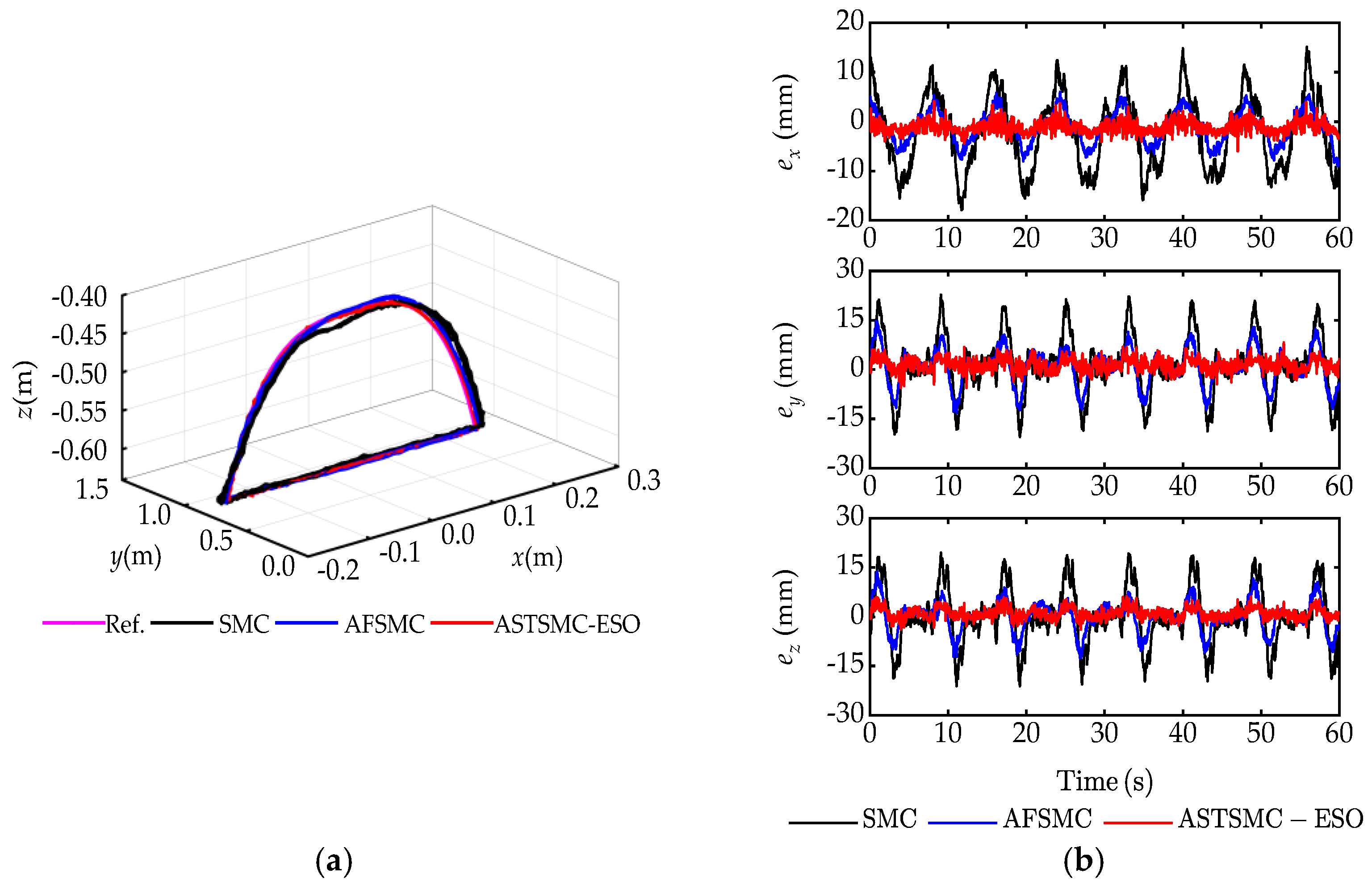
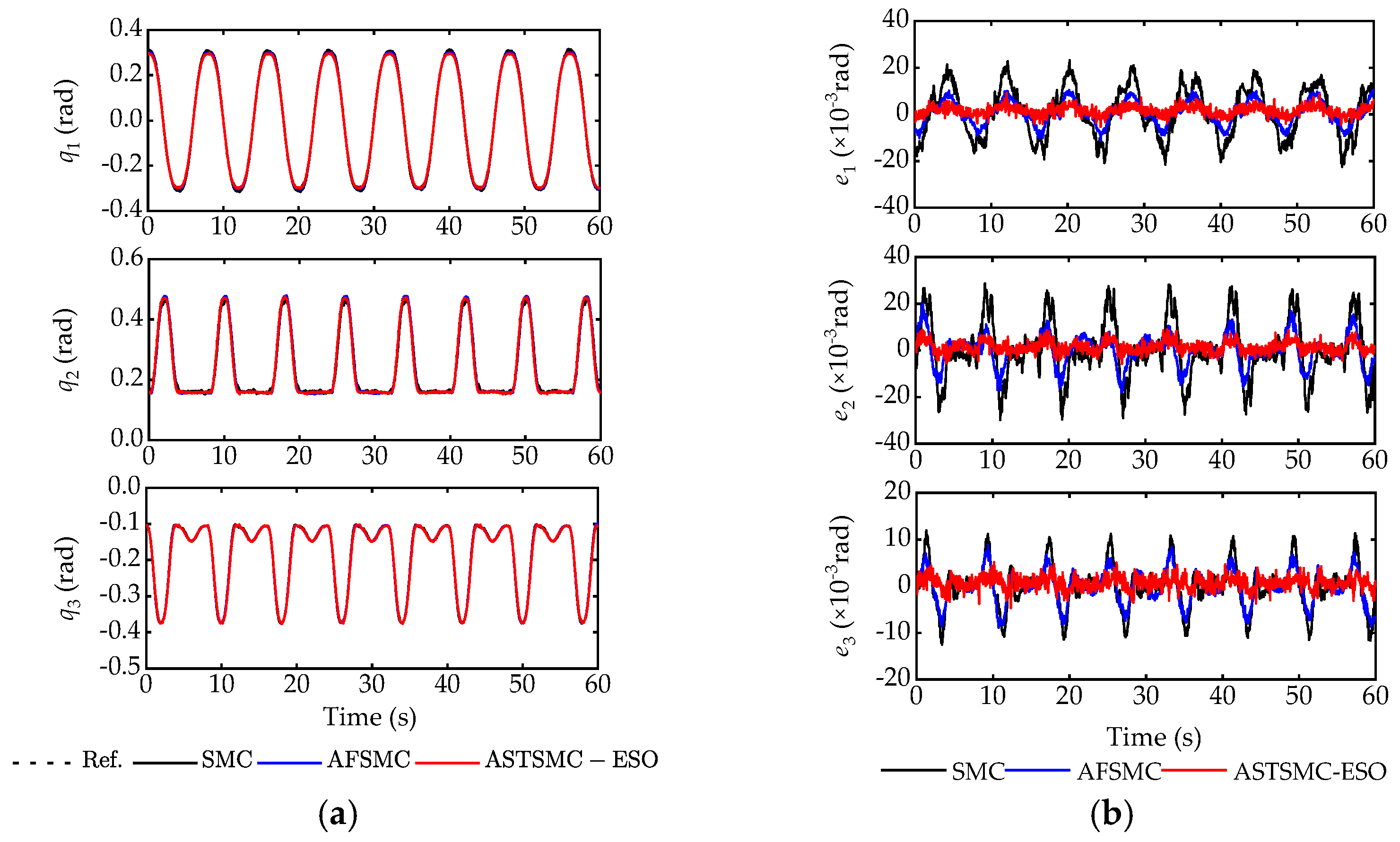
The controller parameters of the experimental study are shown in

Table 6. Controller parameters of the experimental study.

Controller	Parameters
SMC	$\lambda =\mathrm{diag}\left\{400, 600, 600\right\}, k_1=\mathrm{diag}\left\{10, 20, 8\right\}$, $k_2=\mathrm{diag}\left\{150, 180, 100\right\}, \delta =\mathrm{diag}\left\{0.1, 0.1, 0.1\right\}$
AFSMC	$\lambda =\mathrm{diag}\left\{400, 600, 600\right\}, k_1=\mathrm{diag}\left\{10, 20, 8\right\}, \Gamma =\mathrm{diag}\left\{1500, 1500, 1500\right\}$
ASTSMC-ESO	$\lambda =\mathrm{diag}\left\{400, 600, 600\right\}, k_{10}=\mathrm{diag}\left\{10, 20, 8\right\}, k_{20}=\mathrm{diag}\left\{100, 100, 100\right\}$, ${\alpha }_0=\mathrm{diag}\left\{6.32, 6.32, 8.94\right\}, {\beta }_0=\mathrm{diag}\left\{5, 5, 10\right\}, \tau =\mathrm{diag}\left\{0.01, 0.01, 0.01\right\}$, $a=\mathrm{diag}\left\{0.19, 0.19, 0.38\right\}, l_0=\mathrm{diag}\left\{0.5, 0.5, 0.5\right\}, {\rho }_0=\mathrm{diag}\left\{0.5, 0.5, 0.5\right\}$, $\gamma =\mathrm{diag}\left\{0.005, 0.005, 0.005\right\}, {\delta }_0=\mathrm{diag}\left\{80, 80, 80\right\}$, $ϵ=\mathrm{diag}\left\{0.1, 0.1, 0.1\right\}$

. For fairness of comparison, some parameters of ASTSMC-ESO and AFSMC are inherited from the SMC. To evaluate the performance of the three control algorithms, the maximum error $M_e$, average error ${\mu }_e,$ and standard deviation error ${\sigma }_e$ of the foot trajectory were used as indicators [35]. The results are shown in Figure 12, Figure 13 and Figure 14, and the performance evaluation results are listed in

Table 7. Evaluation results of the trajectory tracking performance with different controllers.

Controller	Me (mm)	μe (mm)	σe (mm)
SMC	[17.90, 22.76, 21.15]	[6.42, 6.52, 6.17]	[4.25, 6.05, 5.78]
AFSMC	[8.94, 14.67, 13.73]	[2.79, 4.32, 3.44]	[2.01, 3.91, 3.04]
ASTSMC-ESO	[5.92, 8.28, 6.26]	[1.42, 1.96, 1.54]	[0.91, 1.49, 1.28]

.

The desired foot trajectory and corresponding tracking performance under the three controllers are shown in Figure 12. As seen, the proposed ASTSMC-ESO controller performs better than the other two controllers throughout the movement. From the performance evaluation results in Table 7, it can be seen that all the performance indicators of ASTSMC-ESO are better than SMC and AFSMC. Comparing the joint positions in Figure 13, it can be seen that through uncertainty compensation, the joint position control accuracy can be effectively improved. Further comparing of the joint position errors of ASTSMC-ESO and AFSMC indicates that the former has better robustness than the latter, which is mainly due to the better control mechanism of ASTSMC-ESO than AFSMC.

From Figure 14, we can conclude that the differences in the trajectory tracking performance are mainly due to the differences in the joint control torques of each control method, even though they seem minor. Furthermore, we can see that the torque differences of joint 2 are more significant than those of the other two joints, which are mainly caused by the accuracy of uncertainty compensation, as shown in Figure 14a. AFSMC and ASTSMC-ESO estimate and compensate for the system uncertainties with different methods, so their output control torques can effectively improve the trajectory tracking performance compared with SMC. However, due to the difference in estimation performance, ASTSMC-ESO can compensate for the system uncertainties more precisely than AFSMC, thus further improving the system performance. In addition, it can be seen that the chattering phenomenon of the joint control torques of AFSMC and ASTSMC-ESO is effectively eliminated, which indicates that the AFLS and AST can effectively suppress the chattering effect of SMC while ensuring the control performance of the system.

7. Conclusions

In this paper, a novel adaptive super-twisting sliding mode control method with an extended state observer is proposed for the high-accuracy position control of the UWML in the presence of both uncertainties and external disturbances, which considers the system uncertainties and the external disturbances from the underwater working environment. On the one hand, an accurate model compensation is made with SMC feedback control based on the model information of the UWML to ensure a quick response performance. On the other hand, a feedforward compensation of the system uncertainties is achieved with the estimated uncertainties by ESO to reduce their impact on the control performance. Finally, the AST is introduced to eliminate the chattering phenomenon and further improve the steady-state control accuracy. Simulation and comparative experimental studies were conducted to illustrate the effectiveness of this proposed control scheme, which shows that the proposed controller can effectively compensate for system uncertainties and disturbances and significantly enhance system control accuracy and robustness without the steady-state chattering effect.

References

- Xu, S.; He, B.; Hu, H. Research on Kinematics and Stability of a Bionic Wall-Climbing Hexapod Robot. Appl. Bionics Biomech. 2019, 2019, 6146214. [Google Scholar] [CrossRef]
- Guizzo, E. By leaps and bounds: An exclusive look at how Boston dynamics is redefining robot agility. IEEE Spectr. 2019, 56, 34–39. [Google Scholar] [CrossRef]
- Carlo, J.D.; Wensing, P.M.; Katz, B.; Bledt, G.; Kim, S. Dynamic Locomotion in the MIT Cheetah 3 through Convex Model-Predictive Control. In Proceedings of the 2018 IEEE/RSJ International Conference on Intelligent Robots and Systems (IROS), Madrid, Spain, 1–5 October 2018; pp. 1–9. [Google Scholar]
- Shim, H.; Yoo, S.Y.; Ju, B.H.; Kang, H. Development of arm and leg for seabed walking robot CRABSTER200. Ocean Eng. 2016, 116, 55–67. [Google Scholar] [CrossRef]
- Yang, C.; Yao, F.; Zhang, M.J.; Zhang, Z.Q.; Wu, Z.Z.; Dan, P.J. Adaptive Sliding Mode PID Control for Underwater Manipulator Based on Legendre Polynomial Function Approximation and Its Experimental Evaluation. Appl. Sci. 2020, 10, 1728. [Google Scholar] [CrossRef]
- Yao, J.J.; Wang, C.J. Model reference adaptive control for a hydraulic underwater manipulator. J. Vib. Control 2011, 18, 893–902. [Google Scholar] [CrossRef]
- Lee, M.; Choi, H.S. A Robust Neural Controller for Underwater Robot Manipulators. IEEE Trans. Neural Netw. 2000, 11, 1465–1470. [Google Scholar]
- Zhou, Z.C.; Tang, G.Y.; Huang, H.; Han, L.J.; Xu, R.K. Adaptive nonsingular fast terminal sliding mode control for underwater manipulator robotics with asymmetric saturation actuators. Control Theory Technol. 2020, 18, 81–91. [Google Scholar] [CrossRef]
- Zhou, Z.C.; Tang, G.Y.; Xu, R.K.; HAN, L.J.; Cheng, M.L. A Novel Continuous Nonsingular Finite-Time Control for Underwater Robot Manipulators. J. Mar. Sci. Eng. 2021, 9, 269. [Google Scholar] [CrossRef]
- Chatchanayuenyong, T.; Parnichkun, M. Neural network based-time optimal sliding mode control for an autonomous underwater robot. Mechatronics 2006, 16, 41–87. [Google Scholar] [CrossRef]
- Yao, B.; Tomizuka, M. Adaptive robust motion and force tracking control of robot manipulators in contact with compliant surfaces with unknown stiffness. J. Dyn. Syst. Meas. Control 1998, 120, 232–240. [Google Scholar] [CrossRef]
- Sabanovic, A. Variable structure systems with sliding modes in motion control—A survey. IEEE Trans. Ind. Inform. 2011, 2, 212–223. [Google Scholar] [CrossRef]
- Doulgeri, Z. Sliding regime of a nonlinear robust controller for robot manipulators. IEE Proc. Control Theory Appl. 1999, 146, 493–498. [Google Scholar] [CrossRef]
- Goel, A.; Swarup, A. Adaptive fuzzy high-order super-twisting sliding mode controller for uncertain robotic manipulator. J. Intell. Syst. 2017, 26, 697–715. [Google Scholar] [CrossRef]
- Levant, A. Higher-order sliding modes, differentiation and output-feedback control. Int. J. Control 2003, 76, 924–941. [Google Scholar] [CrossRef]
- Nagesh, I.; Edwards, C. A multivariable super-twisting sliding mode approach. Automatica 2014, 50, 984–988. [Google Scholar] [CrossRef]
- Polyakov, A.; Poznyak, A. Reaching time estimation for ‘‘super-twisting’’ second order sliding mode controller via Lyapunov function designing. IEEE Trans. Autom. Control 2009, 54, 1951–1955. [Google Scholar] [CrossRef]
- Yang, Y.; Qin, S. A new modified super-twisting algorithm with double closed-loop feedback regulation. Trans. Inst. Meas. Control 2017, 39, 1603–1612. [Google Scholar] [CrossRef]
- Boiko, I.; Fridman, L. Analysis of chattering in continuous sliding-mode controllers. IEEE Trans. Autom. Control 2005, 50, 1442–1446. [Google Scholar] [CrossRef]
- Edwards, C.; Shtessel, Y. Adaptive dual-layer super-twisting control and observation. Int. J. Control 2016, 89, 1759–1766. [Google Scholar] [CrossRef]
- Van, M.; Ge, S.S. Adaptive Fuzzy Integral Sliding-Mode Control for Robust Fault-Tolerant Control of Robot Manipulators with Disturbances Observer. IEEE Trans. Fuzzy Syst. 2021, 29, 284–1296. [Google Scholar] [CrossRef]
- Zhu, Y.K.; Qiao, J.Z.; Guo, L. Adaptive Sliding Mode Disturbances Observer-Based Composite Control with Prescribed Performance of Space Manipulators for Target Capturing. IEEE Trans. Ind. Electron. 2019, 66, 1973–1983. [Google Scholar] [CrossRef]
- Xi, R.; Xiao, X.; Ma, T.; Yang, Z. Adaptive Sliding Mode Disturbances Observer Based Robust Control for Robot Manipulators Towards Assembly Assistance. IEEE Robot. Autom. Lett. 2022, 7, 6139–6146. [Google Scholar] [CrossRef]
- Xu, B.; Ji, S.; Zhang, C.; Chen, C.; Ni, H.; Wu, X. Linear-extended-state-observer-based prescribed performance control for trajectory tracking of a robotic manipulator. Ind. Robot Int. J. Robot. Res. Appl. 2021, 48, 544–555. [Google Scholar] [CrossRef]
- Tran, D.T.; Jin, M.; Ahn, K.K. Nonlinear Extended State Observer Based on Output Feedback Control for a Manipulator with Time-Varying Output Constraints and External Disturbances. IEEE Access 2019, 7, 156860–156870. [Google Scholar] [CrossRef]
- Wu, X.; Wang, C.; Hua, S. Adaptive extended state observer-based nonsingular terminal sliding mode control for the aircraft skin inspection robot. J. Intell. Robot. Syst. 2020, 98, 721–732. [Google Scholar] [CrossRef]
- Yao, J.Y.; Jiao, Z.X.; Ma, D.W. Adaptive robust control of DC motors with extended state observer. IEEE Trans. Ind. Electron. 2013, 61, 3630–3637. [Google Scholar] [CrossRef]
- Liao, L.H.; Li, B.R.; Wang, Y.Y.; Xi, Y.; Zhang, D.J.; Gao, L.L. Adaptive fuzzy robust control of a bionic mechanical leg with a high gain observer. IEEE Access 2021, 9, 134037–134051. [Google Scholar] [CrossRef]
- Liao, L.H.; Li, B.R.; Zhang, D.J.; Ngwa, M.; Gao, L.P.; Du, J.M. Research on the Influence of Underwater Environment on the Dynamic Performance of the Mechanical Leg of a Deep-sea Crawling and Swimming Robot. arXiv 2023, arXiv:2308.14393. [Google Scholar]
- Zheng, Q.; Gao, L.; Gao, Z. On stability analysis of active disturbances rejection control for nonlinear time-varying plants with unknown dynamics. In Proceedings of the IEEE Conference on Decision and Control, New Orleans, LA, USA, 12–14 December 2007; pp. 3501–3506. [Google Scholar]
- Yang, Y.J.; Liao, Y.; Yin, D.W.; Zheng, Y.X. Adaptive dual layer fast super twisting control algorithm. Control Theory Appl. 2016, 33, 1119–1127. [Google Scholar]
- Zhang, M.; Guan, Y.; Zhao, W. Adaptive super-twisting sliding mode control for stabilization platform of laser seeker based on extended state observer. Optik 2019, 199, 163337. [Google Scholar] [CrossRef]
- Luo, G.S. Research on Subsea 7 Function Maser-Slave Hydraulic Manipulator and Its Nonlinear Robust Control. Ph.D. Thesis, Zhejiang University, Hangzhou, China, 2013. [Google Scholar]
- Zhong, Y.G.; Yang, F. Dynamic Modeling and adaptive fuzzy sliding mode control for multi-link underwater manipulators. Ocean Eng. 2019, 187, 106202. [Google Scholar]
- Yao, J.Y.; Deng, W.X.; Jiao, Z.X. Adaptive Control of Hydraulic Actuators with LuGre Model-Based Friction Compensation. IEEE Trans. Ind. Electron. 2015, 62, 6469–6477. [Google Scholar] [CrossRef]
- Wang, Z. Adaptive smooth second-order sliding mode control method with application to missile guidance. Trans. Inst. Meas. Control 2017, 39, 848–860. [Google Scholar] [CrossRef]
- Tan, J.; Zhou, Z.; Zhu, X.P.; Xu, X.P. Fast super twisting algorithm and its application to attitude control of flying wing UAV. Control Decis. 2016, 31, 143–148. [Google Scholar]
Figure 1.
The structure of the UWML.
Figure 2.
D-H coordinate systems of the UWML.
Figure 3.
Compensation oil viscous resistance with different rotation speed and pressure.
Figure 4.
Dynamic seal resistance with respect to rotation speeds and pressure.
Figure 5.
The principle of the ASTSMC-ESO controller for the UWML.
Figure 6.
Simulation model of the UWML.
Figure 7.
Foot trajectory tracking results. (a) Foot trajectory; (b) Foot trajectory tracking error.
Figure 8.
Joint position tracking results. (a) Joint position; (b) Joint position tracking error.
Figure 9.
System uncertainty estimation and joint control torque. (a) Uncertainties estimation; (b) Joint control torque.
Figure 10.
Parameter adaptive function .
Figure 11.
The experimental platform of the UWML.
Figure 12.
Foot trajectory tracking results with different controllers. (a) Foot trajectory; (b) Foot trajectory tracking error.
Figure 13.
Joint position tracking results with different controllers. (a) Joint position; (b) Joint position tracking error.
Figure 14.
System uncertainty estimation and joint control torque with different controllers. (a) Uncertainty estimation; (b) Joint control torque.