
Hovering Flight of a Robotic Hummingbird: Dynamic Observer and Flight Tests

Department of Control Engineering and System Analysis, Université Libre de Bruxelles (ULB), CP. 165-55, 50 Av. F.D. Roosevelt, B-1050 Brussels, Belgium
*
Author to whom correspondence should be addressed.
Actuators 2024, 13(3), 91; https://0-doi-org.brum.beds.ac.uk/10.3390/act13030091
Submission received: 4 February 2024
/
Revised: 21 February 2024
/
Accepted: 26 February 2024
/
Published: 27 February 2024
(This article belongs to the Section Aircraft Actuators)
Abstract
:The paper reports on flight tests at hovering of the COLIBRI robot. After a short review of the control model and the stabilization strategy, two different approaches are considered for the attitude reconstruction from the MEMS Inertial Measurement Unit (IMU): the complementary filter and the full-state dynamic observer, implemented in a specially designed flight control board. It is shown that both strategies provide adequate stabilization at hovering in spite of the strong vibration excitation resulting from the flapping of the wings. Moreover, it is shown that the residual wandering due to noise, robot imperfection, etc., can be significantly reduced by a cascade control loop based on the axial and lateral velocities reconstructed by the full-state observer. Experiments show that this approach based on onboard measurements allows for a station keeping as good as that obtained with velocities reconstructed from an external tracking system. The paper also reports endurance tests conducted with two different robot configurations; the maximum flight time observed is 4 min 30 s.
1. Introduction
Mankind has always been fascinated by the agility of small birds and the hummingbird in particular, which is the only one capable of hovering, flying backward and sideways. In the past decade, miniature components (electronic components, MEMS inertial units, high energy-density batteries) have become available, leading to various research projects involving robotic hummingbirds. The problem is difficult, because it involves many different fields such as unsteady aerodynamics, aeroelasticity, mechanism, manufacturing and control. Not many academic projects went as far as flying. An excellent review of ongoing studies in the field of flapping-wing micro air vehicles is available in [1] (see also [2]). Particularly relevant are the impressive Nanohummingbirds [3], developed by Aerovironment with DARPA funding, and the Konkuk university robot [4,5], with a weight of only 15.8 g and a flight autonomy of 9 min.
Our project named COLIBRI is tailless with two membrane wings, of the size of a large hummingbird. A general view of the robot is presented in Figure 1; the left side shows an early version of the robot [6,7,8] with the control board on top of the robot [9]. The right side shows the current configuration where the control board and the two batteries are located at the bottom of the robot. The wing span is 21 cm, the flapping frequency is 20 Hz and the weight is around 22–23 g depending on the configuration. The flapping mechanism and gearbox are documented in [10]. The wings consist of membranes attached to the leading edge bars (moved by the flapping mechanism) and the control bars used to change the membrane wings configuration in order to generate the control torques (the technique called wing twist modulation was pioneered in [3]). All actuators (motor, servos) are low-cost, off-the-shelf components. The robot structure is 3-D printed. The initial version of the COLIBRI robot used a Micro MWC Flight Control Board of Hobbyking with a clock of 16 MHz and a six-axes IMU (three gyro axes and three accelerometer axes), for a weight of 1.8 gr. A new control board has been developed including a ARM processor with a clockspeed of 168 MHz and two IMU sensors, one with six axes and one with nine axes, including a magnetometer. The board also includes a Bluetooth link, for a total weight of 1.4 gr; it is briefly described in [11]. The IMUs are particularly critical components in view of the noisy environment due to the flapping of the wings; the flapping noise is analysed in [11].
It is not difficult to imagine the wide range of applications that a robotic hummingbird could perform if it were available with an agility comparable to that of real birds, particularly the most difficult task of all: reconnaissance in a confined, unstructured environment. On the military side, drones are taking an increasing role in modern warfare; robotic birds would bring the highly desirable feature of concealment (camouflage). But prior to this, one must produce a robot capable of following a trajectory with reasonable accuracy for a sufficient flight time (for comparison, the Black Hornet, a rotorcraft of the size of a small bird popular in the military, has a flight autonomy of 25 min, and a price tag of six digits). The current limit to autonomy is that the mass of existing robotic hummingbirds is still about twice the mass of their natural counterpart with the same wing span [12].
The MEMS inertial unit (IMU) of a flapping wing robot is a critical component because of the intense flapping noise; this motivated researchers to provide the control board with two different IMUs with different full-scale ranges. Each of them consists of three rate gyros measuring the roll-pitch-yaw angular velocity in the robot frame and the three components of the specific acceleration s = a − g (the absolute vector acceleration of the IMU unit minus the gravity vector ). In hovering, and the specific acceleration indicates the position of the gravity vector in the robot frame, from which the robot attitude (roll-pitch) can (in principle) be calculated. However, the acceleration and angular velocity data are subject to intense flapping noise at the flapping frequency and higher harmonics (the harmonic content of the lift and drag forces and the aerodynamic torque is documented in [11], together with a brief description of the control board).
At hovering, the dynamics of the pitch and roll axes of a robotic hummingbird are unstable; they can be stabilized actively if the robot attitude and angular velocities are available (or can be reconstructed) from the IMU. If the pitch and roll references are set to 0, the robot will inevitably drift from the starting position and an additional sensor is required for station keeping (on-board optical flow sensor or external sensor such a video external attitude tracking system). The present study explores an alternative approach based on a dynamic state observer reconstructing the linear forward and lateral velocities.
The present paper is organized as follows: Section 2 briefly recalls the equations governing the cycle-averaged longitudinal and lateral flight dynamics of the robot (they are essentially the same as those used in the simulation paper). Section 3 discusses the feedback stabilization with a PD compensator, assuming a perfect knowledge of the pitch angle and pitch rate q. While the pitch rate is directly available from the gyro, the pitch attitude angle is not. Section 4 considers two different strategies for attitude reconstruction: complementary filter and full-state (Luenberger) observer; both strategies are successful in stabilizing the robot in spite of the strong flapping noise, as reported in the flight tests, Section 5. Additionally, because of the availability of an estimator of the axial velocity in the full-state observer, a PI velocity feedback outer loop significantly improves the station keeping of the hovering robot, with an accuracy comparable with that of earlier tests carried out with an external motion tracking system [6]. Section 6 reports on endurance flights with two different versions of the robot.
2. Flight Dynamics
2.1. Cycle-Averaged Longitudinal Dynamics
Previous studies have shown that, near hovering, the low-frequency dynamics of the hummingbird robot (say, below 10 Hz) can be modelled as a rigid body and that the weak coupling between the longitudinal (pitch) and the lateral (roll) dynamics allows to treat them as independent. The following discussion will be focused on the longitudinal dynamics; a similar treatment applies to the lateral dynamics (with appropriate values of the model parameters). Since the flapping frequency is high compared to the robot dynamics, the complexity of the aerodynamic forces acting on the robot can be ignored and they may be approximated by their cycle-averaged values; a similar approach was followed by [13,14,15]. The rapid change in the aerodynamic moment as well as the lift and drag forces during a flapping cycle will appear as noise. Note that, if the aerodynamic forces along the lateral axis are self-balanced within a flapping cycle (due to left-right symmetry), it is not the case in the longitudinal axis, resulting in a significant pitch torque noise and drag forces. To alleviate this, Delft university has developed a flapper drone with four wings [16] which is also self-equilibrated in the longitudinal axis; this architecture increases the lift with the so-called clap and fling mechanism and it considerably reduces the flapping disturbance. However, such a morphology does not exist in nature.
2.2. Control Model
The longitudinal dynamics near hovering is governed by the Newton-Euler equations. Referring to Figure 2, Newton’s equation reads
where m is the mass of the robot, u is the velocity of the center of mass (CG), is the pitch angle (assumed small, so that and ) and is the pitch velocity. L is the lift (follower) force; at hovering its vertical component balances the gravity force and the component along the body axis is . is the drag force acting at the center of drag (CD) along the body axis .
The main damping mechanism is the flapping of the wings. The complex aerodynamic forces can be modelled by a point force proportional to the velocity of the center of drag located above the center of mass (Figure 2). The position of the center of drag is estimated at a quarter chord from the leading edge at mid-wing. The drag force is proportional to the velocity of the center of drag:
with the constant K being a linear function of the flapping frequency. u is the axial velocity of the center of mass and q is the pitch angular velocity. This model was validated with a set of pendulum experiments and was found to be very accurate [6,17]. It follows that the constants appearing in Equation (1) are and .
Similarly, the rotary motion follows the Euler equation:
where is the moment of inertia about the center of mass; is the drag torque with and . can be estimated also with a pendulum experiment (with the pendulum axis aligned on the center of mass). Direct and fairly accurate measurements of and are available while the cross coupling terms and result from a model and are less accurate; the distance between the center of mass and the center of drag is not known accurately.
The aerodynamic control torque results from the wing twisting obtained by the rotation of the control bars. The latter are operated by servos which can be modelled as first-order systems, so that the actual control torque is related to the requested torque (output of the controller) by
where T is the time constant of the servo. In state-space form, the cycle-averaged longitudinal dynamics read
where and are always negative and and are negative if , that is if the center of drag is above the center of mass, and positive if . The above equation includes the flapping drag noise d and the pitch flapping torque noise that enter the system at the input. Time-histories of the lift L, the drag d and the pitch torque have been studied in experiments reported in [11]. The signals are periodic but very complex, involving a lot of harmonic components and peak values at least one order of magnitude larger than their cycle-averaged values. For example, the RMS value of the aerodynamic torque is 0.0273 N·m (2780 gr·mm) while the (cycle-averaged) control torque that can be achieved by the control bars is limited to 2 N·mm (±200 gr·mm).
Similar considerations apply to the lateral dynamics with significantly lower values of the drag and torque noise because of the symmetry.
3. Stabilization
In short, the axial dynamics of the robot can be written in the classical state space form
where . The matrices A and B are given in Equation (5). w represents the system noise produced by the flapping of the wings, , as discussed above.
The open-loop longitudinal dynamics is unstable and the poles configuration (the eigenvalues of A) depends strongly of the value of . For (center of drag above the center of mass), the system has two unstable oscillatory poles and two poles on the negative real axis (blue × in Figure 3). If one considers the system as a SISO system with the control torque as input and the pitch angle as output, the system can be stabilized with a PD compensator, . This adds a zero in the open-loop system; Figure 3 shows the root locus as a function of the proportional gain . The position of the closed-loop poles corresponding to , 15 mm and is indicated in red [6].
4. Attitude Estimation
The PD compensator discussed above looks satisfactory; however, the pitch angle is not directly available because the IMU MEMS unit consists of three rate gyros measuring the roll-pitch-yaw angular velocity in the robot frame and the three components of the specific acceleration s = a − g, i.e., the absolute vector acceleration of the IMU unit minus the gravity vector .
4.1. Output Equation
In hovering, the absolute acceleration and the specific acceleration indicates the position of the gravity vector in the robot frame, from which the robot attitude (roll-pitch) can be calculated:
For the 1-D model considered here, if the IMU is located at a distance of the center of mass ( if the IMU is above the center of mass and if it is below), the x and z components of the specific acceleration are, respectively,
At hovering, and, because the component is subject to the intense periodic fluctuation of the lift force, may be a more accurate estimator.
From the foregoing discussion, we conclude that the important components of the IMU outputs are (the x component of the accelerometer) and q (the y component of the gyro). Considering the system equation, Equation (5), the output equation relating the sensor output to the state vector reads
in short, . Let us consider two different ways of dealing with the output signal to estimate the pitch attitude angle .
4.2. Complementary Filter
The gyros of the IMU unit provide the pitch rate that can be integrated to obtain an estimator of . However, it is well known that gyros are prone to drift. This can be alleviated by high-pass (HP) filtering.
On the other hand, we have just seen that, at hovering, the MEMS accelerometers provide another estimator, . The sensitivity to the intense high-frequency flapping noise can be alleviated by low-pass filtering (LP).
The idea in the Complementary Filter (CF) consists of combining the output of the two filters above; assuming second order Butterworth filters, the estimator reads
where is the corner frequency of the complementary filter, delimiting the frequency ranges where the accelerometer and the gyro are more reliable. Note that the sum of the two filters, HP + LP, is an all-pass filter.
The system can be looked at as a SISO system with input and output ; its block diagram is shown in Figure 4. The return loop involves three low-pass filters, at on the gyro output, at on the accelerometer output, and in the complementary filter, respectively. is particularly important, because its output is directly used in the construction of the control torque ; it has a direct impact on the stability margins. Extensive numerical studies [11] have shown that Hz offers a good compromise between stability and noise rejection. The frequencies (accelerometer output) and the complementary filter corner frequency are less critical; they have been selected Hz and Hz.
4.3. Full-State Dynamic Observer
The central assumption in the complementary filter is that of hovering, that is, the absolute acceleration is , so that the direction of the gravity vector in the robot frame can be extracted from the accelerometer signal. Since the robot is subjected to a strong flapping noise, an alternative approach consists of including the robot dynamics in the attitude estimation; this approach is advocated by [18] for spacecraft applications. A solution is given by a full-state dynamic observer (Luenberger observer) provided that a reasonably accurate linear state space model is available, Equations (6) and (11) in this case. The reconstructed state is solution of
This equation assumes that the model is accurate; the error follows the equation
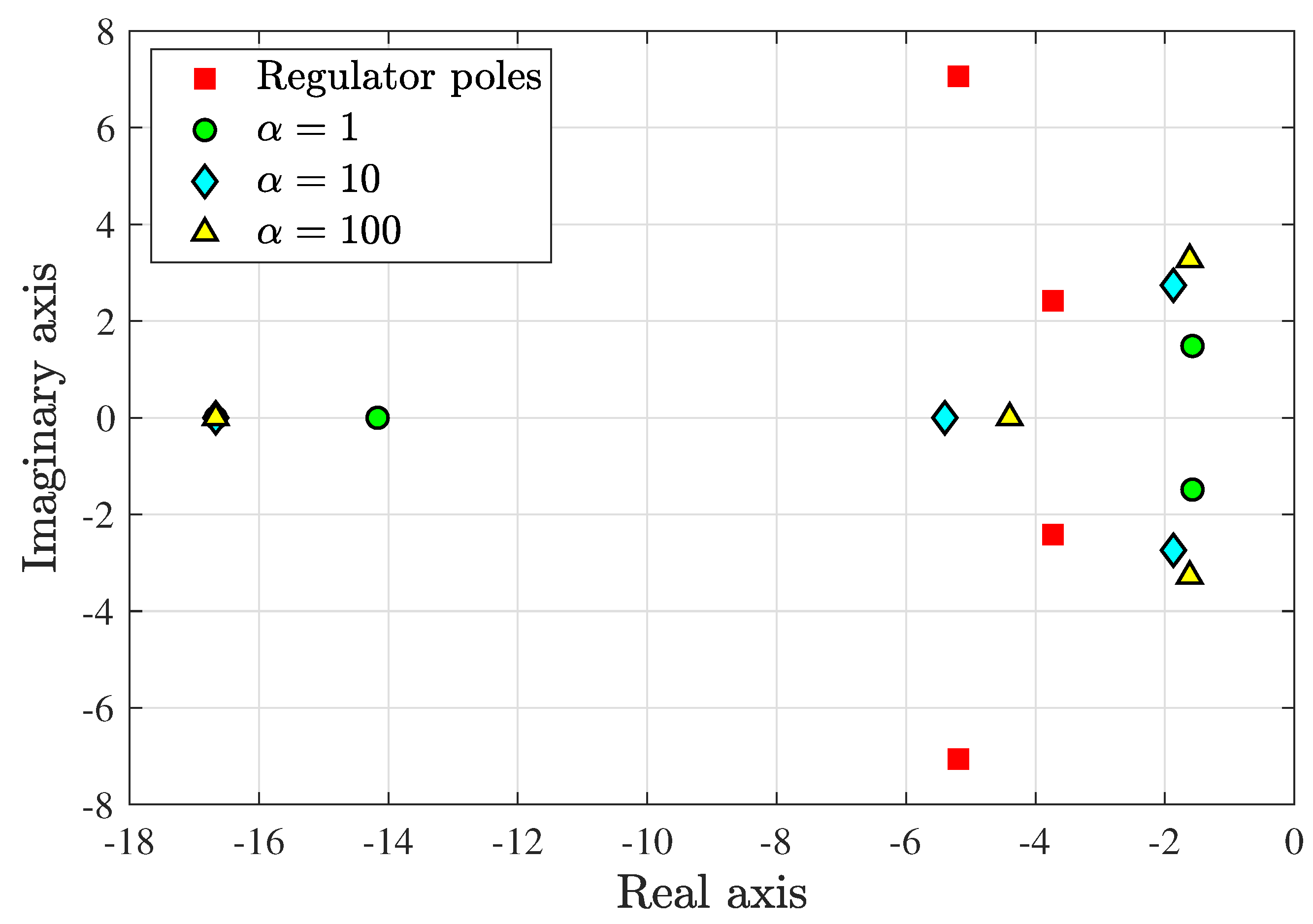
where L is the observer gain matrix, chosen to achieve adequate filtering properties of the IMU signals from the gyro and the accelerometer. According to the separation principle, the closed-loop poles consist of two decoupled sets, corresponding to the full-state feedback regulator (PD in this case) and the full-state observer; the closed-loop stability is guaranteed provided the eigenvalues of have negative real parts. The observer gain matrix may be obtained by pole placement or as a Kalman-Bucy filter, in short, Kalman Filter (KF), assuming that the plant noise w and the sensor noise v are white noise of given covariance matrices, W and V, respectively. This approach is followed here.
4.4. Kalman Filter
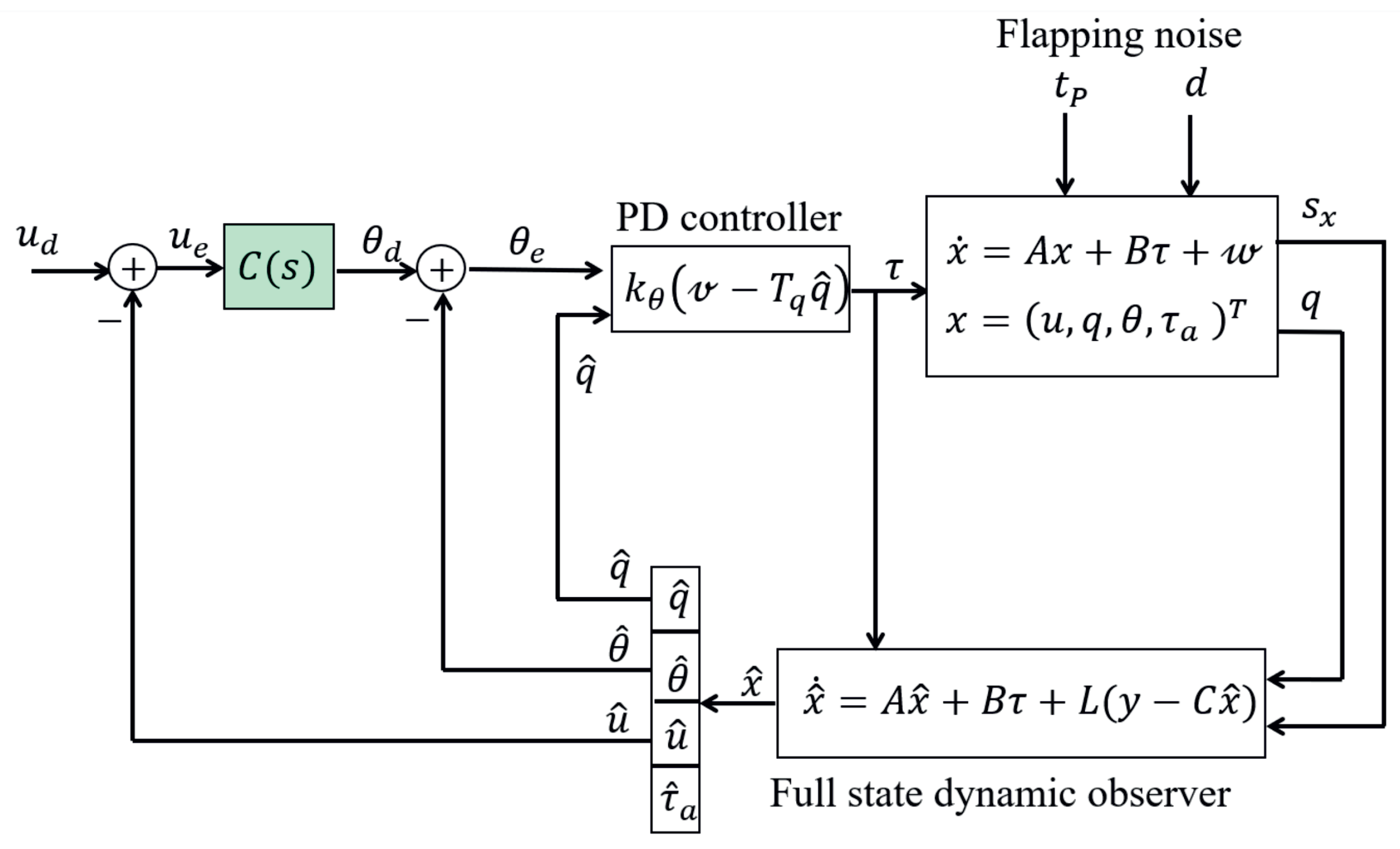
From measurements reported in [11], the variance of the drag noise and the pitch torque noise are estimated: (N/kg)2 and 200,000 (N/kg · m)2 (the components of the plant noise are expressed in different units; in SI units, their ratio is 100). The sensor noise covariance matrix may be estimated from the zero-acceleration output of the accelerometers and the zero-rate output of the gyros, available from the data sheet of the IMU sensor, 0.30 m/s2 and 0.085 rad/s, respectively, leading to (m/s2)2 and (rad/s)2, respectively. Thus the ratio . Figure 5 shows the block diagram of the longitudinal stability control loop with a full-state dynamic observer.
According to the foregoing discussion, we assume the following form for the plant noise W and the sensor noise V covariance matrices:
where is a design parameter. A small value of indicates that low noise measurements may be trusted. Note that only the ratio between V and W matters (multiplying both matrices by a scaler leads to the same gain matrix L). The measurement noise acts as an excitation in the observer error Equation (14), amplified by the observer gain matrix (); as a result, noisy measurements require moderate gains in the observer.
5. Flight Tests
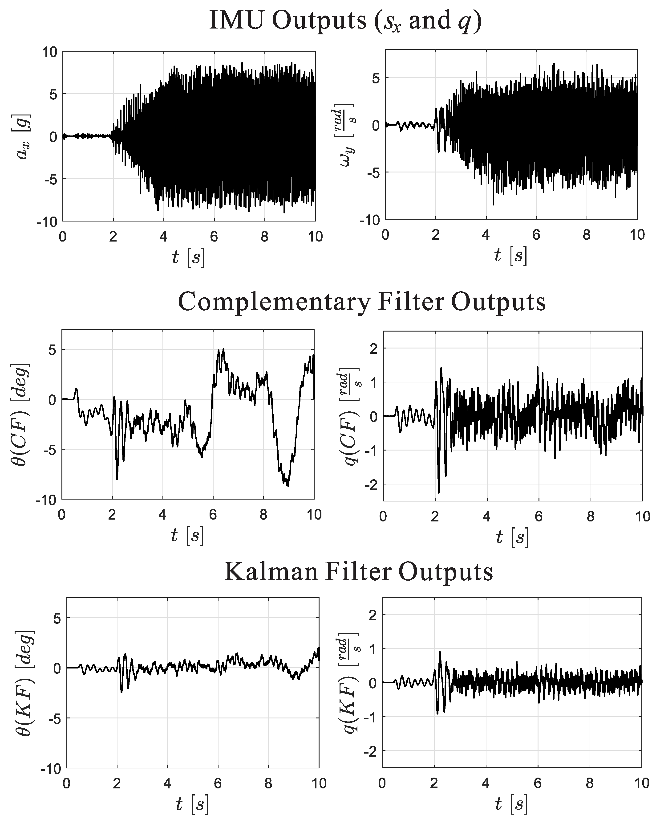
The control strategy explained for stabilizing the pitch (X) axis is applied also for the roll (Y) axis with appropriate values of the parameters of the Kalman filter (the model parameters for X and Y are slightly different, due to differences in the various drag coefficients appearing in the control model). The Complementary Filter (CF) and the Kalman Filter (KF) attitude reconstruction have been implemented in the control board. Attitude stabilization of the robot has been achieved successfully with both methods as illustrated by the video [19]. Figure 7 compares the reconstructed pitch angle and pitch rate of the two filters for a short spell of a stationary flight when the stabilization feedback loop is based on the Kalman Filter. Notice that the accelerometer output has a RMS amplitude of 4.1 g, while a pitch angle of 0.1 rad corresponds to an horizontal component of the gravity acceleration of 0.1 g. This means that the signal to noise ratio is of the order of 1%, which is quite challenging. We have observed that the reconstructed signal from the KF is systematically lower than that reconstructed from the CF, and the same trend has been observed when the stabilization loop is based on CF rather than KF. However, both filters successfully stabilize the robot and no significant visual difference is observed as illustrated in the video [19].
5.1. Station Keeping
When the references of the pitch and roll control loops are set to , the robot does not remain exactly at the same place but slowly drifts away from its starting position due to small inaccuracies in the IMU calibration, the strong flapping noise, the imperfect symmetry between the forward and backward strokes, etc. [19]. The Kalman filter reconstructs the full state that includes the forward velocity u (and the lateral velocity v). If the signal reconstruction is good enough, a cascaded control of the linear velocity may be implemented as shown in Figure 8. The compensator transforms the velocity error into a pitch angle demand with a P+I compensator:
where the parameters and have been selected after numerical simulations to provide adequate stability margins [11], and finally adjusted from flight tests. The proposed strategy looks fairly straightforward, but it was not obvious that it would work in practice, given the severe flapping noise affecting the IMU sensor. The flight tests have shown that it works as one can see one the short video [20]. The left side of Figure 9 compares trajectories of the center of mass of the robot with (in red) and without (in blue) velocity control measured by an external tracking system. The right side of the figure shows similar measurements conducted earlier when the velocity used in the feedback was that reconstructed from the external tracking system [6]. This figure shows similar performances of the two approaches; the on-board measurements allows to keep the robot within a circle with a radius of about one wingspan.
5.2. Yaw Control, Trajectory Generation
The control configuration shown in Figure 8 is exactly the configuration needed to generate the axial and lateral components of the robot trajectories. However, a careful observation of the videos reveal that the robot slowly rotates about the yaw axis. This is due to the fact that, to speed-up the research, the current versions of our demonstrator do not include an actuator to control the yaw axis, which is necessary for a full control of the trajectory.
The yaw axis is naturally stable (it is damped by the flapping of the wing); its control has been investigated in [21]. Unlike the pitch and roll torques which are generated by lift modulation, the yaw torque results from differential drag obtained by modifying slightly in opposite directions the central position of the left and right control bars. Once this step is achieved, the magnetometer included in one of the two IMU units in the control board can be used to steer the front axis of the robot and generate trajectories. This step remains to be performed.
6. Endurance Flight
Two prototypes have been built and tested, that differ by the mechanical structure of the flapping wing mechanism (both have the same kinematics), the gear ratio G of the gearbox between the d.c. motor and the flapping mechanism and the wing size W (which affects the lift-frequency relationship and the pitch and roll control moments), Table 1. Two sets of batteries have been considered with the characteristics of Table 2. In each case, two batteries are connected in series. All tests were performed with the same d.c. motor with the characteristics (at room temperature) of Table 3.
The two prototypes were first tested on a load cell with an external power supply; the voltage e and current I necessary to achieve a lift equal to the weight were measured (Table 4). The average current needed for the control board and the two attitude control servos was also estimated to 0.19 A, so that the total current supplied by the battery is A. Table 4 also provides estimates of the electrical power of the motor , the heat power and the mechanical power (necessary to produce the lift and overcome the internal friction in the mechanism and the motor) .
Figure 10 shows the discharge curve of two batteries B1 connected in series. The ∘ indicate the data from the manufacturer for A and the continuous lines correspond to the best-fit Shepherd model [22] for the requested current of the prototypes P1 and P2 (the requested current i is obtained by adding the current needed for the board and attitude servos to the values given in the third column of Table 4, A). The minimum voltage to operate the control board and the servos is 6 V, so the expected operating time with a constant current is obtained when the Shepherd model drops below 6 V.
In the flight tests, the operator adjusts the duty factor of the PWM of the main motor in order to keep a nearly constant altitude (lift equal to weight). When the available voltage at the battery v is larger than the requested voltage e, the duty factor of the PWM of the d.c. motor (i.e., the fraction of time when the full available voltage is applied) is set to . It follows that the total flight time may be estimated by
Table 5 summarizes the results for the two prototypes and the two sets of batteries. is the constant current discharge time obtained from Shepherd’s model, and T is the flight time estimate from Equation (17). is the actual flight time measured. P1-B1 refers to the string mechanism with the first set of batteries; the flight stopped after 106 s because of overheating of the main motor (the energy of the battery was not exhausted). As a result, the flight P1-B2 became useless and was canceled. The flight P2-B1 (gear mechanism) lasted 168 s, well below the estimated s; at least part of the discrepancy can be attributed to the fact that the set of batteries B1 had been used for a long time. The flight P2-B2 is the longest so far, s (nearly 4 min 30 s).
From Table 5, one sees that prototype P1 is subject to overheating in spite of a specific power W/kg while the prototype P2 flies longer with a specific power of 136 W/kg. The reason lies into the following relation between the heat power and the mechanical power [10]:
The first term is motor characteristics (Table 3), the second depends on the gear ratio G and the third one depends on the flapping frequency f. According to this equation, . On the other hand, previous studies have shown that, for a given lift, the mechanical power is to a large extent independent on the wing size (see Figure 6 of [10]). This means that a larger gear ratio and smaller wings (leading to a larger flapping frequency) will reduce heat production. The excess value of the specific power of the gear mechanism as compared to the string mechanism hints that internal friction could be reduced by more accurate components and careful assembly.
7. Conclusions
The attitude reconstruction of a hovering flapping wing robot has been analyzed with a complementary filter and a full-state dynamic observer. Both methods have been successfully implemented and tested, in spite of the high noise environment due to the flapping of the wings. In addition, it was found that the full-state observer allows the reconstruction of the forward and the lateral velocities needed for station keeping and full control of the robot trajectory.
Endurance tests were conducted with two different robot configurations; the maximum flight time observed is 265 s (4 min 30 s) in spite of some parasitic friction in the geared flapping mechanism. Future studies will be devoted to the control of trajectories and increasing the flight time of the robot.
Author Contributions
Conceptualization, A.P., H.W., Y.F. and L.W.; software, Y.F., L.W. and H.W.; test and validation, H.W., L.W. and Y.F.; writing—original draft preparation, A.P.; writing—review and editing, A.P. and Y.F.; supervision, A.P. and E.G. All authors have read and agreed to the published version of the manuscript.
Funding
This research received no external funding.
Institutional Review Board Statement
Not applicable.
Informed Consent Statement
Not applicable.
Data Availability Statement
Data are contained within the article.
Acknowledgments
The authors wish to thank Gert Geboers from Dekimo n.v. for his careful work in the manufacturing of the control board and his availability and help in the initial phase of programming. Many thanks also to Lorenzo Brancato, enthusiastic MSc student of Politecnico di Milano, who contributed to the programming and the early tests in the project during his Erasmus internship at ULB.
Conflicts of Interest
The authors declare no conflicts of interest.
Abbreviations
The following abbreviations are used in this manuscript:
| ARM | Advanced RISC Machine |
| CD | Center of drag |
| CF | Complementary Filter |
| CG | Center of mass |
| DARPA | Defense Advanced Research Projects Agency |
| HP | High Pass filter |
| IMU | Inertial Measurement Unit |
| KF | Kalman Filter |
| LP | Low pass filter |
| MEMS | Micro Electro Mechanical System |
| NA | Non Available |
| PD | Proportional plus Derivative |
| PI | Proportional plus Integral |
| PWM | Pulse Width Modulation |
| RMS | Root Mean Square |
| SI | International System Units |
| SISO | Single Input Single Output |
References
- Xiao, S.; Hu, K.; Huang, B.; Deng, H.; Ding, X. A Review of Research on the Mechanical Desig of Hoverable Flapping Wing Micro-Air Vehicles. J. Bionic Eng. 2021, 18, 1235–1254. [Google Scholar] [CrossRef]
- Ward, T.A.; Rezadad, M.; Fearday, C.J.; Viyapuri, R. A Review of Biomimetic Air Vehicle Research: 1984–2014. Int. J. Micro Air Veh. 2015, 7, 375–394. [Google Scholar] [CrossRef]
- Keennon, M.T.; Klingebiel, K.R.; Won, H.; Andriukov, A. Development of the nano hummingbird: A tailless flapping wing micro air vehicle. In Proceedings of the 50th AIAA Aerospace Sciences Meeting including the New Horizons Forum and Aerospace Exposition, Nashville, TN, USA, 9–12 January 2012; pp. 1–24. [Google Scholar]
- Phan, H.V.; Park, H.C. Insect-inspired, tailless, hover-capable flapping-wing robots: Recent progress, challenges, and future directions. Prog. Aerosp. Sci. 2019, 111, 100573. [Google Scholar] [CrossRef]
- Phan, H.V.; Aurecianus, S.; Au, T.K.L.; Kang, T.; Park, H.C. Towards Long-Endurnce Flight of an Insect-Inspired, Tailess, Two-Winged, Flapping-Wing Flying Robot. IEEE Robot. Autom. Lett. 2020, 5, 5059–5066. [Google Scholar] [CrossRef]
- Roshanbin, A. Design and Development of a Tailless Robotic Hummingbird. Ph.D. Thesis, Université Libre de Bruxelles, Dept Control Engineering and System Analysis, Bruxelles, Belgium, September 2019. [Google Scholar]
- Roshanbin, A.; Altartouri, H.; Karasek, M.; Preumont, A. COLIBRI: A Hovering Flapping Twin-Wing Robot. Int. J. Micro Air Veh. 2017, 9, 270–282. [Google Scholar] [CrossRef]
- Roshanbin, A.; Abad, F.; Preumont, A. Kinematic and Aerodynamic Enhancement of a Robotic Hummingbird. AIAA J. 2019, 57, 4599–4607. [Google Scholar] [CrossRef]
- Colibri Maiden Flight. Available online: https://www.youtube.com/watch?v=-5-o9tvbziE (accessed on 3 February 2024).
- Preumont, A.; Wang, H.; Kang, S.; Wang, K.; Roshanbin, A. A Note on the Electromechanical Design of a Robotic Hummingbird. Actuators 2021, 10, 52. [Google Scholar] [CrossRef]
- Farid, Y.; Wang, L.; Brancato, L.; Wang, H.; Wang, K.; Preumont, A. Robotic Hummingbird Axial Dynamics and Control near Hovering: A Simulation Model. Actuators 2023, 12, 262. [Google Scholar] [CrossRef]
- Greenwalt, C.H. Hummingbirds; Dover: New York, NY, USA, 1990. [Google Scholar]
- Van Breugel, F.; Regan, W.; Lipson, H. From Insects to Machines. IEEE Robot. Autom. Mag. 2008, 15, 68–74. [Google Scholar] [CrossRef]
- Ristroph, L.; Ristroph, G.; Morozova, S.; Bergou, A.J.; Chang, S.; Guckenheimer, J.; Wang, Z.J.; Cohen, I. Active and passive stabilization of body pitch in insect flight. J. R. Soc. Interface 2013, 10, 20130237. [Google Scholar] [CrossRef] [PubMed]
- Teoh, Z.E.; Fuller, S.B.; Chirarattananon, P.; Pérez-Arancibia, N.O.; Greenberg, J.D.; Wood, R.J. A Hovering Flapping-Wing Microrobot with Altitutde Control and Passive Upright Stability. In Proceedings of the 2012 IEEE/RSJ International Conference on Intelligent Robots and Systems, Vilamoura-Algarve, Portugal, 7–12 October 2012; pp. 3209–3216. [Google Scholar]
- Karásek, M.; Muijres, F.T.; De Wagter, C.; Remes, B.D.; De Croon, G.C. A tailess aerial robotic flapper reveals that flies use torque coupling in rapid banked turns. Science 2018, 361, 1089–1094. [Google Scholar] [CrossRef] [PubMed]
- Altartouri, H.; Roshanbin, A.; Andreolli, G.; Fazzi, L.; Karásek, M.; Lalami, M.; Preumont, A. Passive stability enhancement with sails of a hovering flapping twin-wing robot. Int. J. Micro Air Veh. 2019, 11, 1756829319841817. [Google Scholar] [CrossRef]
- Yang, Y.; Zhou, Z. Attitude determination: With or without spacecraft dynamics. Adv. Aircr. Spacecr. Sci. 2017, 4, 335–351. [Google Scholar]
- CF and KF Stabilization Loop. Available online: https://youtu.be/ZCN5RK5Thb0 (accessed on 3 February 2024).
- Station Keeping. Available online: https://youtu.be/53DJ0rtebKk (accessed on 3 February 2024).
- Roshanbin, A.; Preumont, A. Yaw control torque generation for a hovering robotic hummingbird. Int. J. Adv. Robot. Syst. 2019, 16, 1–14. [Google Scholar] [CrossRef]
- Shepherd, C.M. Design of Primary and Secondary Cells-Part 2. An Equation Describing Battery Discharge. J. Electrochem. Soc. 1965, 112, 657–664. [Google Scholar] [CrossRef]
Figure 1.
The robot COLIBRI. Left: early version with the control board on top [7]. Right: current configuration with the control board at the bottom. (1) Flight control board, (2) batteries, (3) main motor, (4) gearbox and flapping mechanism, (5) attitude control actuators.
Figure 1.
The robot COLIBRI. Left: early version with the control board on top [7]. Right: current configuration with the control board at the bottom. (1) Flight control board, (2) batteries, (3) main motor, (4) gearbox and flapping mechanism, (5) attitude control actuators.

Figure 2.
Longitudinal (pitch) model of the robot near hovering. Coordinate system, force and moment diagram.
Figure 2.
Longitudinal (pitch) model of the robot near hovering. Coordinate system, force and moment diagram.

Figure 3.
Root-locus plot trajectories as a function of the proportional feedback gain for PD control of the robot with and mm. The open-loop poles and zero are the blue ×. The red squares indicate the closed-loop poles location obtained with .
Figure 3.
Root-locus plot trajectories as a function of the proportional feedback gain for PD control of the robot with and mm. The open-loop poles and zero are the blue ×. The red squares indicate the closed-loop poles location obtained with .

Figure 4.
Block diagram of the longitudinal stability control loop with a complementary filter. is the requested control torque, is the position of the servo actuator acting on the control bars and is the actual torque produced by the flapping wings, including the periodic noise components.
Figure 4.
Block diagram of the longitudinal stability control loop with a complementary filter. is the requested control torque, is the position of the servo actuator acting on the control bars and is the actual torque produced by the flapping wings, including the periodic noise components.

Figure 5.
Block diagram of the longitudinal stability control loop with a full-state dynamic observer. The symbols have the same meaning as in the previous figure.
Figure 5.
Block diagram of the longitudinal stability control loop with a full-state dynamic observer. The symbols have the same meaning as in the previous figure.

Figure 6.
Observer poles for 1, 10 and 100 (the pole on the left side of the real axis is common to all values of ). The regulator poles of Figure 3 are also shown with red squares.
Figure 6.
Observer poles for 1, 10 and 100 (the pole on the left side of the real axis is common to all values of ). The regulator poles of Figure 3 are also shown with red squares.

Figure 7.
Comparison of the outputs of the Complementary Filter (CF: in Figure 4) and the Kalman Filter (KF: in Figure 5) in a short interval of a stationary flight () when the stabilization feedback loop is based on the Kalman Filter output. The upper figures refer to the IMU outputs ().

Figure 8.
Cascaded control on the linear velocity u. The flapping noise includes the drag d and the pitch torque .
Figure 8.
Cascaded control on the linear velocity u. The flapping noise includes the drag d and the pitch torque .

Figure 9.
Comparison of trajectories with and without velocity control. Left: velocity control based on the reconstruction from the on-board sensor and Kalman filter. Right: velocity control based on an external tracking system [6].
Figure 9.
Comparison of trajectories with and without velocity control. Left: velocity control based on the reconstruction from the on-board sensor and Kalman filter. Right: velocity control based on an external tracking system [6].

Figure 10.
Discharge curve of two batteries B1 in series for a the discharge rate of 1.2 A (data from manufacturer) and the best-fit Shepherd model. The other curves correspond to the Shepherd model for the discharge currents of the two prototypes.
Figure 10.
Discharge curve of two batteries B1 in series for a the discharge rate of 1.2 A (data from manufacturer) and the best-fit Shepherd model. The other curves correspond to the Shepherd model for the discharge currents of the two prototypes.


Table 1.
Characteristics of the prototypes considered in this study.
| Prototype | Flapping | Gearbox | Wing Size | Weight | Flapping |
|---|---|---|---|---|---|
| Number | Mechanism | Ratio G | W (mm) | L (gr) | Frequency f (Hz) |
| P1 | String | 28.9 | 88 | 22 | 18 |
| P2 | Gear | 39 | 81 | 22.6 | 19 |
Table 2.
Characteristics of the batteries.
| Battery | Reference | Capacity | Discharge | Weight | Max. |
|---|---|---|---|---|---|
| Number | (mAh) | Rate | (gr) | Current (A) | |
| B1 | Hyperion G5 | 70 | 25C–30C | 2.26 | 1.75–2.1 |
| LiPo | (50C burst) | ||||
| B2 | Honcell | 95 | 15C | 2.3 | 1.425 |
Table 3.
Characteristics of the d.c. motor.
| Producer | Weight (gr) | (Ω) | k ( V.s) | () |
|---|---|---|---|---|
| Micronwings | 3.51 | 0.76 | 7.18 | 0.0147 |
Table 4.
Flight characteristics of the robots.
| Prototype | Operating | Operating | Electrical | Heat | Mechanical |
|---|---|---|---|---|---|
| Number | Voltage | Current | Power | Power | Power |
| P1 | 3.2 | 1.12 | 3.58 | 0.95 | 2.63 |
| P2 | 3.92 | 0.97 | 3.80 | 0.715 | 3.08 |
Table 5.
Estimated and measured flight time, specific power .
| Prototype | Shepherd | Estimated | Actual | Remark | |
|---|---|---|---|---|---|
| Battery | Equation (17) | Flight | (W/kg) | ||
| P1-B1 | 130 s | 279 s | 106 s | 119 | Overheating |
| P1-B2 | - | - | - | - | - |
| P2-B1 | 150 s | 265 s | 168 s | 136 | Old batteries |
| P2-B2 | NA | NA | 265 s | 136 | Longest flight |
Disclaimer/Publisher’s Note: The statements, opinions and data contained in all publications are solely those of the individual author(s) and contributor(s) and not of MDPI and/or the editor(s). MDPI and/or the editor(s) disclaim responsibility for any injury to people or property resulting from any ideas, methods, instructions or products referred to in the content. |
© 2024 by the authors. Licensee MDPI, Basel, Switzerland. This article is an open access article distributed under the terms and conditions of the Creative Commons Attribution (CC BY) license (https://creativecommons.org/licenses/by/4.0/).
Share and Cite
MDPI and ACS Style
Wang, H.; Farid, Y.; Wang, L.; Garone, E.; Preumont, A. Hovering Flight of a Robotic Hummingbird: Dynamic Observer and Flight Tests. Actuators 2024, 13, 91. https://0-doi-org.brum.beds.ac.uk/10.3390/act13030091
AMA Style
Wang H, Farid Y, Wang L, Garone E, Preumont A. Hovering Flight of a Robotic Hummingbird: Dynamic Observer and Flight Tests. Actuators. 2024; 13(3):91. https://0-doi-org.brum.beds.ac.uk/10.3390/act13030091
Chicago/Turabian StyleWang, Han, Yousef Farid, Liang Wang, Emanuele Garone, and André Preumont. 2024. "Hovering Flight of a Robotic Hummingbird: Dynamic Observer and Flight Tests" Actuators 13, no. 3: 91. https://0-doi-org.brum.beds.ac.uk/10.3390/act13030091
Note that from the first issue of 2016, this journal uses article numbers instead of page numbers. See further details here.