

In-Flight Calibration of Lorentz Actuators for Non-Contact Close-Proximity Formation Satellites with Cooperative Control


Institute of Astronautics, Nanjing University of Aeronautics and Astronautics, Nanjing 211106, China
*
Author to whom correspondence should be addressed.
Actuators 2024, 13(4), 129; https://0-doi-org.brum.beds.ac.uk/10.3390/act13040129
Submission received: 8 February 2024
/
Revised: 31 March 2024
/
Accepted: 1 April 2024
/
Published: 3 April 2024
(This article belongs to the Section Aircraft Actuators)
Abstract
:The non-contact close-proximity formation satellite (NCCPFS) is one of the technical solutions to improve the attitude performance, consisting of a payload module (PM) and a support module (SM). The non-contact Lorentz actuator (NCLA), as the core components of the NCCPFS, directly affect the attitude control performance of the entire satellite. In order to ensure the ultra-high attitude pointing performance and stability of the PM, an in-flight calibration method for the NCLAs based on minimum model error (MME) algorithm and Kalman filtering (KF) with cooperative control strategy is proposed in this article. In this method, the NCLAs generate a periodic nominal torque that causes the attitude of the PM to be periodically deflected. This periodic torque also reacts on the SM, and the SM counteracts this periodic torque through the flywheel to realize the cooperative tracking relative to the PM. Then, the gyroscope data are substituted into the MME algorithm to obtain the angular acceleration of the two modules, and the KF algorithm is adopted to observe the actual output torque of the NCLAs to complete the in-flight calibration of the NCLAs. Numerical simulation results show that the accuracy of the proposed calibration algorithm can reach about 8%, which proves the effectiveness of the proposed method.
1. Introduction
As the complexity of future space missions continue to increase, modern satellite payloads such as high-resolution remote sensing, high-resolution radar, and space telescopes become more sophisticated [1], putting higher demand on the pointing accuracy and stability of satellite attitude control systems [2,3]. To reduce the impact of flexible and moving components of the satellite on the pointing accuracy and stability of the payload, the concept of a non-contact close-proximity formation satellite (NCCPFS) has been proposed by Pedreiro [4]. This concept divides the satellite into a payload module (PM) and a support module (SM), which are connected by non-contact Lorentz actuators (NCLA) to achieve complete isolation between the PM and the disturbance source [5,6], effectively improving the PM’s attitude control performance.
The structure design of NCCPFS two-module close-proximity formation implies that it is necessary to choose a cooperative control strategy to avoid any collision between two modules. The cooperative control strategy designed in this article is mainly divided into two parts: the active attitude control loop for the PM and a passive attitude control loop for the SM. The PM uses NCLAs as its attitude execution mechanism, while the SM uses flywheels to achieve attitude tracking of the PM.
NCLAs, with advantages such as fast response times and high accuracy, are the core components of NCCPFS [7] and are crucial for achieving high-precision attitude control [8,9], which has already established relatively mature structural configurations and control strategies after years of research and development [10,11]. NCLAs are the attitude controller of PM, and its internal excitation coils generate periodic control torques based on a uniform magnetic field to act on the PM. Although NCLAs can be pre-calibrated on the ground, in practical in-flight applications, the control performance of the NCLAs is affected by factors such as material out-gassing, relative coupling between the positions and attitudes of the two modules under micro-gravity, non-uniformity of the magnetic field caused by the space magnetic field, and uncertainty in the installation matrix of the NCLAs due to measurement limitations. Therefore, to eliminate the system errors caused by the in-flight space environment on the NCLAs, it is necessary to accurately calibrate the output torque of the NCLAs in-flight.
Significant progress has been made by domestic and international researchers on calibration algorithms. Yuan proposed calibration model based on continuous acquisition of satellite attitude information, which has higher attitude determination performance compared to traditional calibration models [12]. Cheng applies the unscented Kalman filter (UKF) to the single-axis rotational inertial navigation system by introducing the external position reference, achieving the comprehensive calibration method of nonlinear filter estimation [13], which has certain feasibility in engineering applications. Lin proposes an enhanced automatic traditional tool center point calibration method based on a laser displacement sensor and implemented on a cooperative robot with six degrees of freedom [14]. Hammer designed a calibration scheme for measuring the internal magnetometer data of celestial bodies based on the CryoSat-2 satellite’s in-flight data. This scheme considers the magnetic interference caused by the battery, solar cells, and magnetic torques on the measurement data [15]. Pittelkau obtained the absolute standard error model and gyroscope error model using the Kalman filtering (KF) algorithm and derived the noise matrix for the calculation process based on this model [16]. Szabo proposed a calibration method to calculate the position iteratively based on two observations, greatly reducing the number of steps required for calibration [17].
Due to the lack of reliable angular acceleration sensor, the data of measurement equation of the in-flight calibration cannot be obtained directly. To address this issue, this article adopts the minimum model error (MME) algorithm, which was proposed by Mook [18]. Based on the optimal control theory, Mook introduced the Pontryagin maximum principle into nonlinear estimation problems, which defines the unknown part of the model as model error, thus the MME algorithm does not require knowledge of the mathematical model of the variables to be estimated [19]. To eliminate the systematic error of the model, this article adopts the KF algorithm, which iteratively calculates the current optimal state estimate by combining the current measurements with the previous estimated state values until the iteration results reach the accuracy requirement [20]. By combining these two algorithms, the model error generated by the sensors in the mathematical model and the desired angular acceleration can be simultaneously estimated, avoiding the influence of attitude input errors on calibration accuracy.
The main contributions of this article can be outlined as follows.
- (1)
- Having noticed that most of the existing calibration methods for NCLAs are carried out on the ground, this article proposes a NCLA in-flight calibration method.
- (2)
- This article designs a two-module close-proximity formation cooperative control strategy, which the angular acceleration is estimated by MME algorithm and the final results are filtered by the KF algorithm to improve accuracy.
The rest of this article is organized as follows. The overall design of NCCPFS is given in Section 2. Section 3 presents the design of calibration architecture. The calibration algorithm is described in Section 4. In Section 5, numerical simulation is performed to demonstrate the validation of the algorithm. Finally, the main conclusions are drawn in Section 6.
2. Hierarchical Architecture
2.1. Overall Structure
The design concept of the NCCPFS is different from traditional satellite structures. It separates the satellite into two independent yet organically combined parts—the PM and the SM—through the use of the NCLAs. The two modules are separated from each other through the electromagnetic force in the NCLAs while still being able to maintain relative motion so that there is no physical connection between the two modules. This cuts off the physical contact between the noisy module and the quiet module, achieving the purpose of dynamic and static isolation.
The structure of the NCCPFS is shown in Figure 1. The PM mainly installs the components that require vibration isolation such as telescopes, radars, cameras, as well as sensitive elements like star sensors and gyroscopes. The SM mainly installs the power component, attitude component, and communication component. The power component is solar sails, the attitude component includes thrusters and flywheel, and the communication component includes antennas and a data transmission receiver. The flexibility of solar sails and antennas as well as the vibration generated by thrusters and flywheels during operation will greatly impact the ultra-stable control of high-precision payloads [21]. Therefore, in order to isolate the influence of interfering factors on the PM, the two modules are connected by eight orthogonally mounted NCLAs, which generate Lorentz forces that act on both the PM and the SM. The control system of the SM is basically the same as the traditional satellite control system, and the attitude of the PM is used as the reference for tracking control. During the in-flight maneuvering, the two modules will both rotate around the center of mass of the PM to avoid collision. Obviously, these NCLAs serve as the execution units for PM attitude control and relative position control between the two modules. When the PM is in motion, the SM will track the attitude of the PM using flywheels. To maintain the relative position between the two modules and avoid collisions, the NCLAs will generate Lorentz forces on the PM, synthesizing control moments to drive the rotation of the PM.
To ensure the long-term dynamic and static isolation effect between the PM and the SM, the NCCPFS must ensure that the relative positions between the PM and the SM follow a certain range. Therefore, this article adopts a cooperative control strategy by using the PM as a reference and having the SM follow the PM. In order to reduce the coupling between the active control of the PM and the passive control of the SM, this article uses an eight-rod NCLA with a minimum-norm decoupling strategy.
NCLAs are the core of high-precision attitude control for the PM, and their output performance directly affects the satellite’s attitude control. In addition, different NCLA layout schemes will also affect the difficulty in controlling the output force of the actuator and the complexity of the coupling between the actuators, making it necessary to study the structure and layout scheme of the NCLA.
2.2. Non-Contact Actuator
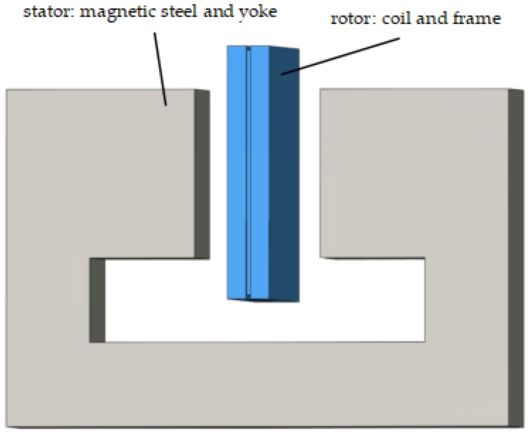
In order to achieve physical isolation between the two modules, a reasonable non-contact mechanism must be adopted. NCLA has the advantages of fast response, high accuracy, simple structure, and convenient installation. Therefore, this article chooses it as the actuator for the PM [22]. Its structural diagram is shown in Figure 2.
The working principle of a NCLA is the generation of Lorentz force by energized coils in a magnetic field. The NCLA is mainly composed of the stator and the rotor (Figure 2). The stator is composed of magnetic steel and yoke, while the rotor consists of a coil and a frame. The stator is installed on the SM, and the rotor is installed on the PM, with no physical contact between the stator and the rotor. Due to the micro-gravity environment of NCCPFS’s in-flight, NCLA is less perturbed under normal conditions. Therefore, maintaining the non-contact state of the rotor and stator in space does not require additional magnetic levitation force.
The total force generated by the NCLA in the magnetic field is the control force of the PM. The force exerted on an individual NCLA in the magnetic field can be expressed as:
where B is the magnetic induction intensity, l is the length of the coil in the magnetic field, θ is the angle between the magnetic bar and the magnetic field, f is the Lorentz force, i is the energizing current, and k is the driving parameter.
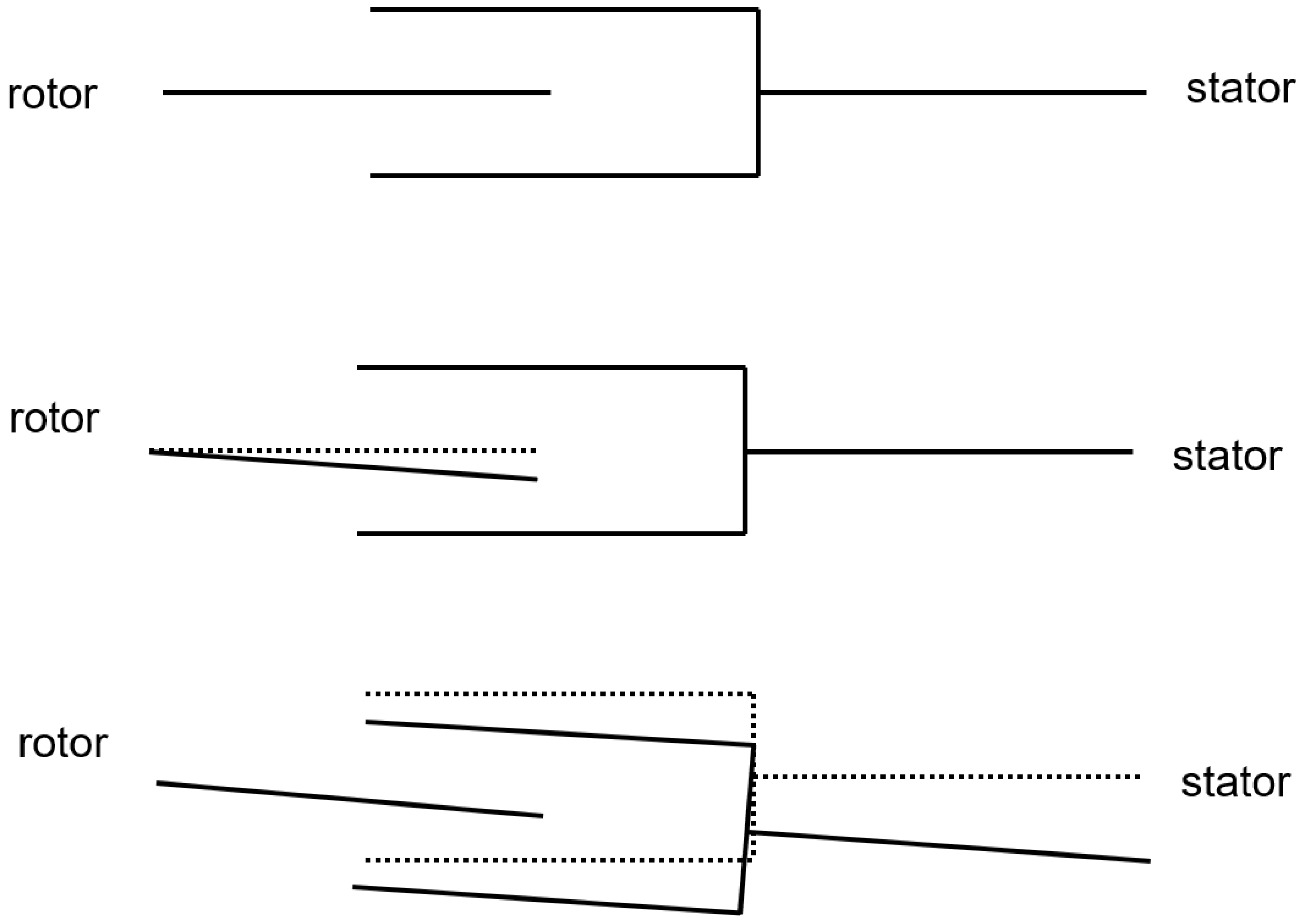
The movement process of NCLA is shown in Figure 3.
It can be seen from Figure 3 that the rotor of NCLA is equipped with a stator in PM and a stator in SM. During control, the drive control circuit of rotor outputs current and the rotor cuts the magnetic field in stator to generate control information to actively control the PM. At the same time, its reaction force also acts on the stator, that is, the SM. At this point, the SM flywheel controls the SM to move around the PM.
The layout scheme of NCLAs and the force generated is shown in Figure 4.
The installation positions of the eight NCLAs are shown in Figure 4, with the stator of each NCLA mounted on the SM and the rotor mounted on the PM. The direction of magnetic induction intensity generated by the stators A1, A2, A3, and A4 are perpendicular to the satellite installation plane. The direction of magnetic induction intensity generated by the stators B1, B2, B3, and B4 are parallel to the satellite installation plane. Eight NCLAs are symmetrically arranged, with each NCLA only generating forces along one of the x, y, or z axes. By A1, A2, A3, and A4, the rotation of the PM around the x direction is realized. The rotation of the PM around the y direction is realized by A1, A2, A3, and A4. The rotation of the PM around the z direction is realized by B1, B2, B3, and B4.
In this structure, by using minimum norm decoupling, the control force of each NCLA can be determined uniquely and definitively [23], and there are no singularities. Correspondingly, the control current corresponding to this control force can be calculated through the force constant of the NCLA, achieving a fully decoupled control of the PM attitude and the relative positions of the two modules in the system. The PM attitude is adjusted by attitude control force, and the relative positions of the two modules are adjusted by relative position control force. Additionally, the decoupling of the satellite control force is simple, making the control simple.
Remark 1.
The distribution of the output force can be achieved through minimum norm decoupling, but the decoupling is effective only when the force output of NCLA is accurate, so the performance of NCLA output force directly affects the smooth execution of in-flight missions. However, although the output force of NCLA can be calibrated on the ground, in actual in-flight applications, the control performance of the NCLA is affected by issues such as material out-gassing, relative coupling between the position and attitude of the two modules in micro-gravity, non-uniformity of the magnetic field caused by the space magnetic field, and the uncertainty of the installation matrix of the NCLA due to measurement methods [24]. Therefore, to ensure the effectiveness of the NCLA in-flight, it is necessary to accurately calibrate the output.
3. Calibration Architecture Design
3.1. Dynamic Model
The premise of the in-flight calibration is to establish the coordinate system and dynamic model that meet the requirements of the satellite attitude control. It can be seen from Section 2 that the special connecting structure between the two modules of the NCCPFS lead to the requirement of establishing an effective two-module cooperative control strategy.
As shown in Figure 5, the establishment of the satellite attitude motion model involves the following coordinate systems: J2000.0 Earth-centered inertial coordinate system, PM orbit coordinate system, PM body coordinate system, and SM body coordinate system [22].
The definitions of these four coordinate systems are as follows:
- (1)
- J2000.0 Earth-centered inertial coordinate system:
J2000.0 Earth-centered inertial coordinate system Fi:O-XiYiZi, where the origin O is located at the Earth’s core. The OXi axis points to the vernal equinox of the year 2000 on the intersection line between the ecliptic plane and the Earth’s equatorial plane. The OZi axis points towards the North Pole, and the OYi axis satisfies the right-hand rule, forming a right-handed Cartesian coordinate system.
- (2)
- PM orbit coordinate system:
Orbit coordinate system Fpo: O-XpoYpoZpo, where the origin O is at the satellite’s center of mass. The OZpo axis points towards the Earth’s center, OXpo axis lies in the orbital plane and has the same direction as the satellite’s velocity, and OYpo axis, together with the OZpo and OXpo axes, form a right-handed system.
- (3)
- PM body coordinate system:
Body coordinate system Fpb: O-XpbYpbZpb, where the origin O is located at the center of the PM, coinciding with the origin of the orbit coordinate system. The OXpb, OYpb, and OZpb axes are fixed to the PM body and represent the three principal axes of inertia for the PM. Specifically, the OXpb axis corresponds to the roll axis, the OYpb axis corresponds to the pitch axis, and the O Zpb axis corresponds to the yaw axis.
- (4)
- SM body coordinate system:
SM body coordinate system Fsb: O-XsbYsbZsb, similar to the PM body coordinate system, origin O is located at the center of the SM. The OXsb, OYsb, and OZsb axes are fixed to the SM body and represent the three principal axes of inertia for the SM.
In this article, the two-module dynamic modeling of the satellite can be divided into two parts: the active dynamic model of the PM and the follow-up dynamic model of the SM [25]. The PM can be regarded as a rigid body, so its dynamic model has the same structure as the rigid satellite dynamic model. The SM follows the attitude of the PM, so its dynamic model has the same structure as the PM dynamic model. However, because the reference coordinate system is different, there is a formal difference between them.
The PM adopts active control, with the orbit coordinate system as the reference coordinate system. The attitude kinematics model of the PM relative to the orbit system is:
where qpo is the quaternion representing the attitude of the PM relative to the orbit system and is the angular velocity of the PM body relative to the orbit system.
The absolute angular velocity vector of the PM body coordinate with respect to the inertial coordinate is . The motion of the PM relative to the inertial coordinate can be divided into two parts: the motion of the PM relative to the orbital coordinate and the motion of the orbital coordinate itself, thus:
where is the angular velocity of the orbital coordinate, with respect to the inertial coordinate. The formula is projected into the PM body coordinate, therefore:
where is the coordinate transformation matrix from the orbital coordinate to the PM body coordinate.
The attitude dynamics model of the PM under the PM body coordinate can be obtained:
Since the actual engineering background of this article is a near circular orbits, the term is insignificant, thus:
By bringing it into the above equation, the orbital dynamics equation of the PM is obtained:
where Jp is the moment of inertia of the PM, is the angular velocity of the orbit system relative to the inertial system, is the absolute angular velocity of the PM relative to the inertial system, is the coordinate transformation matrix from the orbit system to the PM body system, Tcp is the control torque applied to the PM, Tdp is the disturbance torque acting on the PM.
The SM is under passive control, with the PM coordinate system as the reference coordinate system. When the PM maneuvers, the SM tracks the PM’s attitude and rotates around the PM. The attitude kinematics and dynamics model of the SM relative to the PM is similar to the aforementioned equation:
where Js is the moment of inertia matrix of the SM, Jfw is the moment of inertia matrix of the flywheel, qsp is the quaternion representing the attitude of the SM relative to the PM, is the absolute angular velocity vector of the SM relative to the inertial system, is the rotational velocity of the SM relative to the PM project to the SM coordinate body system, is the rotational velocity of the flywheel project to the SM body coordinate system, is the transformation matrix from the PM to the SM, Tds is the disturbance torque acting on the SM, and Tcs is the control torque applied to the SM.
3.2. Calibration Method with Cooperative Control
Prior to the in-flight calibration of the NCLAs, there is no relative motion or interaction between the two modules. The NCCPFS ought to be stabilized relative to the body coordinate system or three-axis stabilized to the earth. For the consideration of the satellite in-flight, such as earth imaging [26], the three-axis stabilization is chosen in this article. The schematic diagram of NCLA’s control force in-flight calibration scheme is shown in Figure 5.
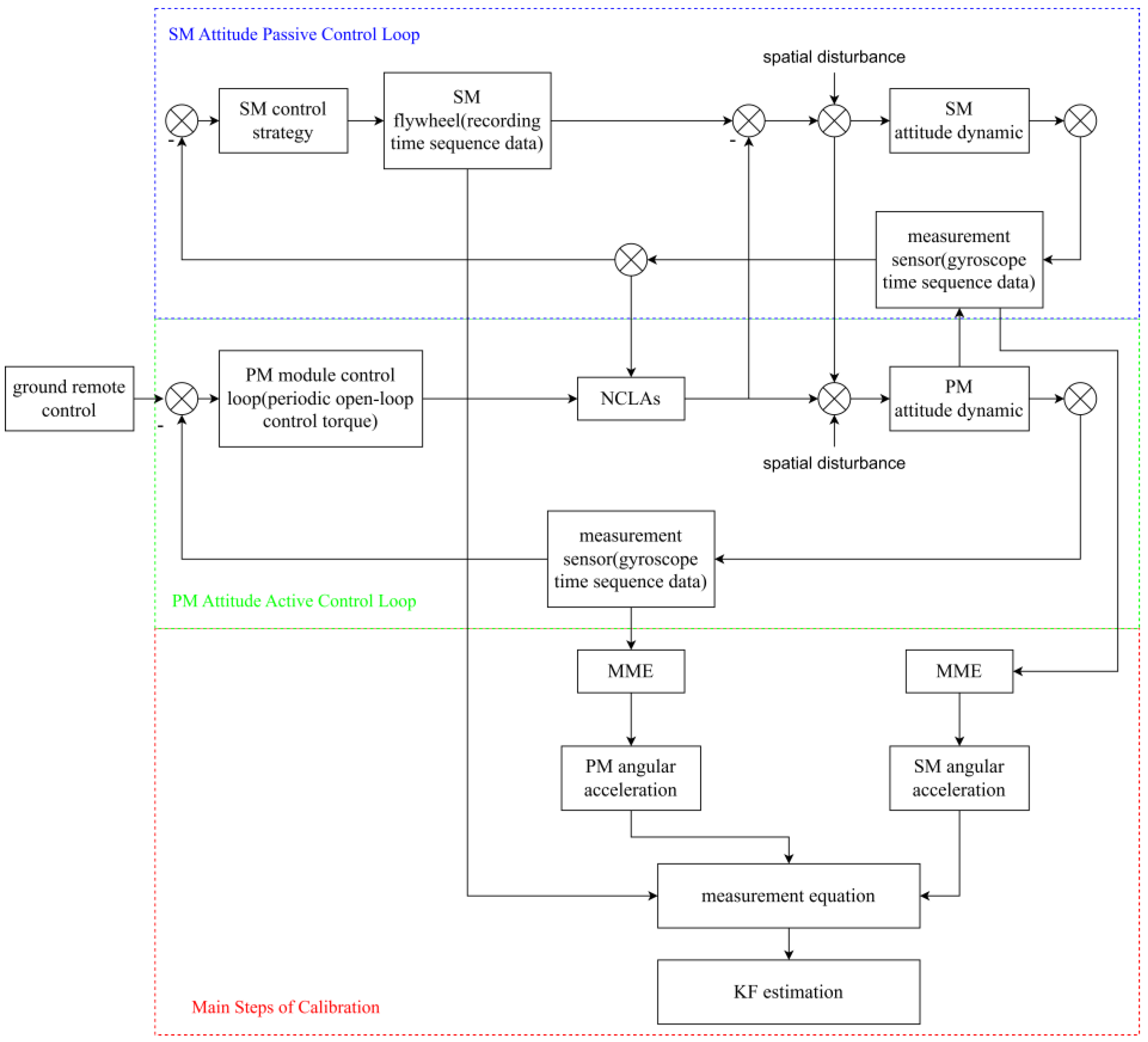
As shown in Figure 6, an attitude control command is sent to the NCLAs to generate periodic control torques acting on the PM, causing changes in the PM’s attitude. In order to maintain relative attitude stability between the two modules, the SM generates the corresponding control torque through the flywheel to adjust its attitude and compensates for the environmental disturbance torque to realize passive control. In this way, we can acquire the calibrated measurement equations and state equations.
Successfully completing the above in-flight calibration plan requires an effective NCCPFS two-module cooperative control loop. The schematic diagram of the control loop established in this article is shown in Figure 6, which can be divided into three parts.
Figure 7 shows that the object studied in our article is the cooperative movement of two modules of the twin-body satellite rather than the traditional multi-star formation flight, yet in our design, the PM is the reference, which installs the star-sensors and gyroscopes as the measurement references. According to the measurement information, PM moving first is realized through the NCLAs control torque generated by the coil of the NCLAs and the magnetic steel. The control system of the SM is basically the same as traditional satellite control system, and the attitude of the PM is used as the reference for tracking control. Therefore, the active control loop for the attitude of the PM is used to generate periodic open-loop control torque, causing changes in the attitude of the PM and recording the timing data of the PM gyroscope. In order to enable the PM’s dynamic model to have fast response capability and strong robustness, the design of the control torque in this article adopts the PD control, which is widely used in engineering [27].
where Kpp and Kdp are the PD controller parameters of the PM, respectively.
This article proves the stability of the above PD controlled. First, the Lyapunov equation is constructed as follows:
where Jp is the inertial tensor matrix.
From the quaternion property , it can be seen that . Both Jp and Kpp in the equation are positively definite, therefore the Lyapunov function is globally positively definite.
Taking the derivative of Lyapunov function over time yields, there is:
The scalar part of a quaternion is , and substituted into the Equation (12), thus:
According to Lyapunov theorem, when the Lyapunov equation is not greater than 0, that is, the energy stored in the system is continuously decaying with time, it is considered that the trajectory of any initial condition near the equilibrium state of the dynamic system can be maintained near the equilibrium state. So, it can be concluded that the system is stable under the selected control law. Therefore, the attitude of the PM can be stabilized through PD control.
The SM attitude passive control loop performs passive control on the SM to ensure that it can keep up with the PM and records the timing sequence output torque of the SM flywheel and the timing sequence data of the SM gyroscope. Recording the output torque of the flywheel gyroscope is the way to obtain the calibrations’ measurement equation and state equation. To follow the attitude of the PM, the SM is designed with the following controller for passive control:
where Kps and Kds are the PD controller parameters of the SM, respectively. is the vector part of the SM’s attitude quaternion under the SM body coordinate system.
The stability proof process of the SM is similar to the PM, and it will not be repeated here. The SM can also maintain stability by using PD control. In the calibration process, the relative position of the two modules is not significantly changed, so it will be not considered here.
The main steps of calibration are to call the gyroscope angular velocity time sequence data of the PM and SM, respectively, combining the minimum model error estimation method to obtain the angular acceleration of each module, and obtain the timing sequence control torque of the NCLAs through the Kalman filter algorithm.
During the in-flight calibration of the NCLAs, the attitude dynamic equation of the SM is shown in Equation (9). The SM achieves attitude tracking of the PM through the NCLAs. Based on the PM state data, SM state data, and relative state data between the two modules, the calibration torque Tsp(tk) acting on the SM can be calculated as:
Remark 2.
It is obvious that in constructing the above measurement equation, the angular acceleration information of the two modules is required. Since it is difficult to directly obtain the angular acceleration information due to the lack of measurement sensitive elements. In this article, the MME algorithm is introduced into the problem to obtain the angular acceleration information of the two modules during the in-flight calibration of NCLA. Finally, to eliminate the system noise, the centroid positions of the PMs and SMs are estimated using the KF estimation algorithm, which is selected for its efficiency, accuracy, and real-time capability. Both algorithms are well applied in precision parameter calibration in other fields [28,29]. The specific process is described in the following text.
4. Calibration Algorithm Design
4.1. MME-Based Angular Acceleration Estimation
Due to the limitation of engineering conditions, the attitude dynamic characteristics of satellite obtained by current measurement instruments are not entirely reliable. Therefore, using previous dynamic equations to calculate the satellite’s angular acceleration results in significant deviations from the actual situation. This article utilizes the MME algorithm, treating the unknown part of the mathematical model of the variables to be estimated as model errors , by estimating and solving to obtain the satellite’s angular acceleration data. Therefore, the MME algorithm does not require knowledge of the mathematical model of the variables to be estimated.
The estimation of PM angular acceleration (similarly for the SM) based on the MME algorithm is as follows:
where is the estimated value of the PM angular acceleration, is the estimated value of the model error, ωobs is the measurement information from the gyroscopes installed on the PM, Rw is the covariance matrix of the measurement information from the gyroscopes, is the estimated value of the PM angular velocity, and W is a third-order model weighting matrix that continuously adjusts to make the estimated angular velocity consistent with the measured values from the gyroscopes.
Define
Then, Equations (16)–(21) can be expressed as follows:
where:
where M, M0, and Mm represent the boundary conditions. The specific meaning of Dk and Gk represent jump discontinuity.
The matrix containing the angular acceleration information is shown in the following equation:
4.2. KF-Based In-Flight Calibration
The KF algorithm is widely used in engineering state estimation problems. Its basic idea is to estimate the system’s state by fusing the measurements and predictions of the system’s model. It iteratively calculates the current optimal state estimate by combining the current measurements with the previous estimated state values.
For in-flight calibration of the NCLAs, the parameter matrix to be estimated is denoted as AT(tk). The in-flight calibration steps are shown in Figure 8.
The control torque generated by the NCLAs can be expressed as:
where both L and D are 3 × 8 matrices representing the installation positions and directions of the NCLAs in the PM coordinate system, F(tk) represents the thrust magnitude generated by each NCLA at time tk, and AT(tk) is the control torque matrix of the NCLAs at time tk. The purpose of in-flight calibration of the NCLAs is to obtain the mean estimate of AT(tk).
By combining Equations (9), (15), and (32), the measurement equation for the in-flight calibration problem of the NCLAs can be represented as:
where v(tk) represents external disturbance torques and measurement noise.
Let the state variables to be estimated be X = AT(tk), the measurement values be , and the state and measurement equations be as follows:
The main steps of the KF algorithm include prediction and update. In the prediction step, the current state variables and the uncertainty of the state are predicted based on the system’s dynamic model and the previous state estimate. In the update step, the system’s measurements are compared with the estimates, and the state estimate and uncertainty are updated through weighted averaging. The goal of this algorithm is to obtain the true parameter matrix of the NCLAs. The specific iteration process is shown in Equations (36)–(41).
Given the initial estimate of the state variables and the initial estimate covariance matrix P(t0), the one-step prediction formula for the state variables is:
where is the state transition matrix, which is an identity matrix.
Based on the previous posterior covariance matrix P(tk−1), the one-step estimate error covariance matrix P(tk/k−1) is:
Then, the Kalman gain matrix K(tk) for this iteration is calculated as:
where R(tk) is the covariance matrix of the measurement noise v(tk) and H(tk) is the measurement transition matrix, which is composed of the attitude control commands Dc(tk).
The updated estimate error covariance matrix for this iteration is given by:
This prepares for the next computation.
Finally, the optimal mean estimate of the state variables for this iteration, which corresponds to the optimal mean estimate of the NCLA parameter matrix, is obtained as:
In order to verify the effectiveness of the KF algorithm in this article, two performance evaluation parameters are introduced: filtering error and filtering accuracy, which are described in the following [32]:
The filter error is defined as:
Under the same conditions, the smaller Er(tk) is, the better the filtering effect is. Starting from the filtering stability moment tk0, k1 consecutive sampling points are taken for analysis. The filtering accuracy is defined as:
The smaller the filtering accuracy Er, the better the filtering effect.
Since there are many formula symbols in this article, for ease of understanding, the meanings of all symbols used in the above formula can be found in Table 1.
5. Simulation Results
5.1. Initial Conditions
The objective of this simulation is to achieve successful in-flight calibration of the center of mass position between the PM and the SM, as well as collision avoidance control of the attitude between the two modules. The initial conditions for the simulation are shown in Table 2.
Selecting PD control parameters that are too large can cause the system’s output value to oscillate and fail to converge. Choosing parameters that are too small can result in a longer response time and slow response to input signal changes, making it difficult to achieve stability [33]. Therefore, it is necessary to choose PD control parameters within a reasonable range to ensure that there is no collision between the two modules. The selected control parameters for the control gains in this article are shown in Table 3.
5.2. Validation of the Effectiveness of Cooperative Control
The torque exerted by the NCLAs on the PM is shown in Figure 9, with consistent torques applied in the three-axis directions.
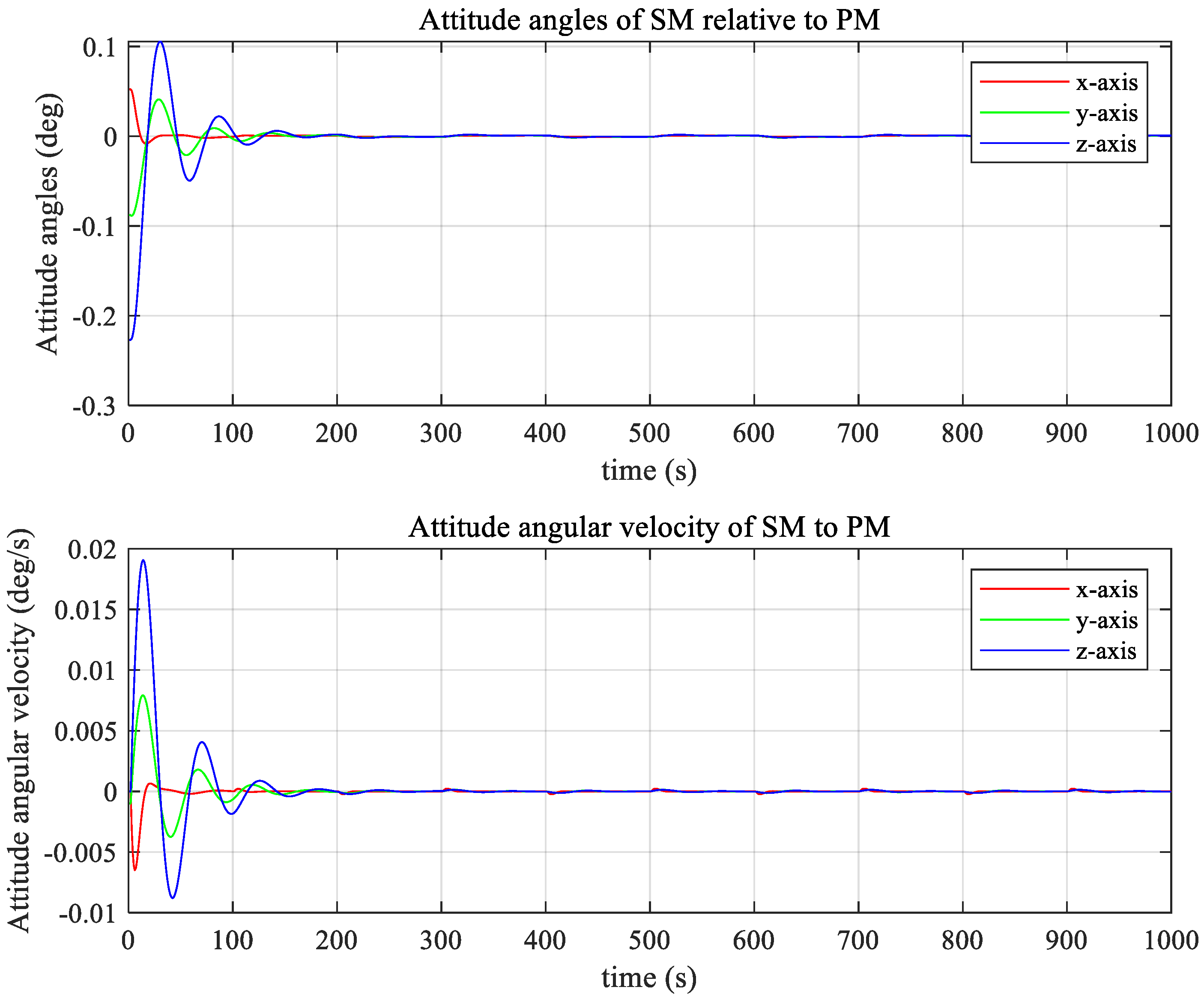
The dynamics information of the two modules in the calibration process are shown in Figure 10, Figure 11 and Figure 12.
According to the information in the figures above, the oscillations of the relative distance, relative angle, and angular velocity of the two modules are all in a very small range and can reach a convergence state within 200 s. As such, we can judge that the PD control based cooperative control strategy which was selected in this article is effective.
5.3. Calibration Accuracy Verification
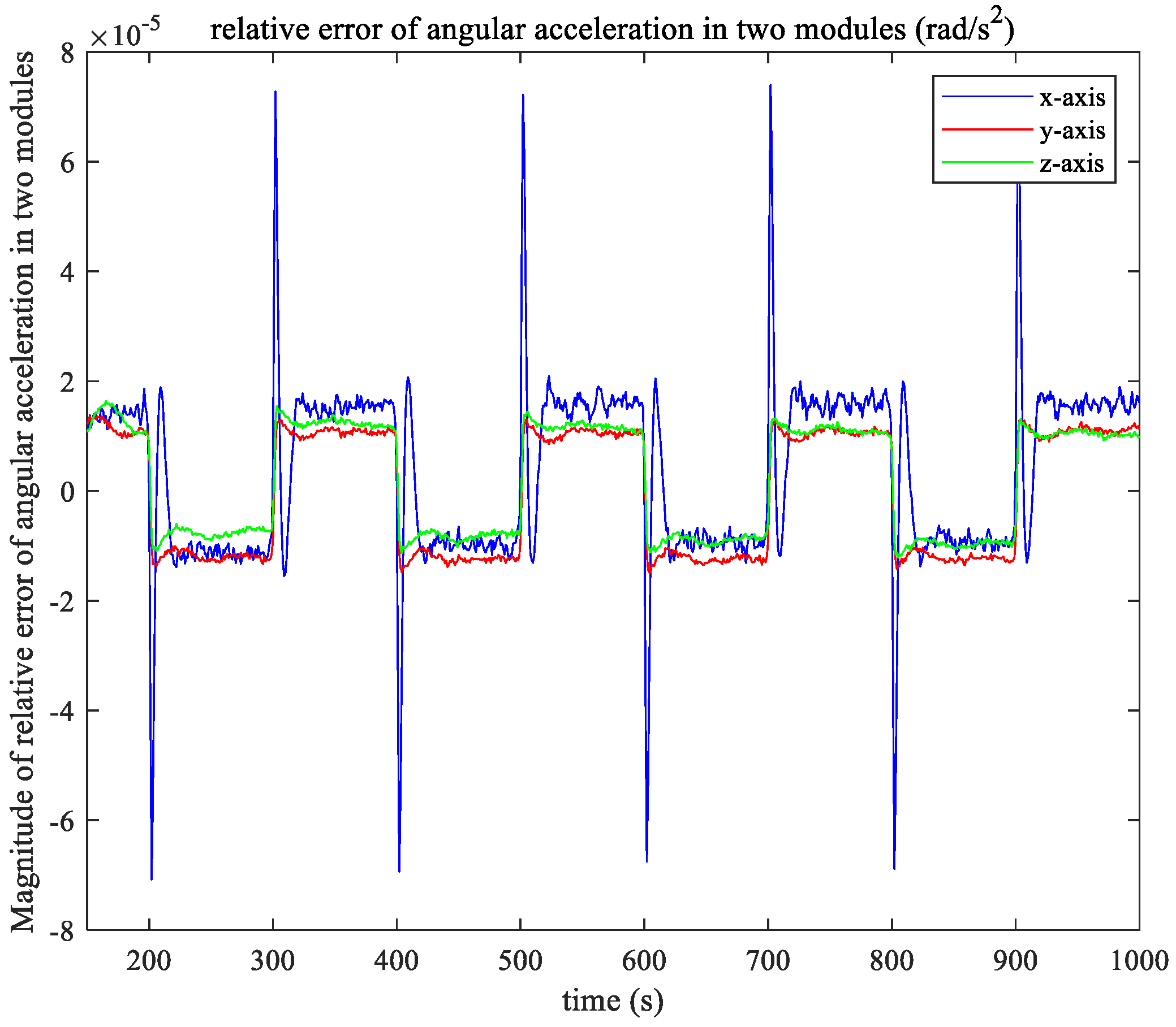
The error between the angular acceleration of the PM estimated by the MME algorithm and the actual measured value of the angular acceleration can be seen in Figure 13, and the error of the angular acceleration of the two modules can be seen in Figure 14.
It can be seen from the calibration simulation results that the accuracy of the estimated angular acceleration of the PM and the relative error accuracy of the two modules angular acceleration are both in the order of 10−5. This means that the algorithm based on MME/KF can successfully acquires the calculation of the centroid motion of the two modules even without exact attitude information.
Figure 15 shows the simulation results of the in-flight calibration error percentage of the NCLA. It can be observed that the calibration error accuracy in all three axes can be maintained at a level of 8%, so the algorithm successfully performs the calibration calculation of the centroid motion of the two modules of the NCCPFS. As can be seen in Figure 16, the magnitudes of filtering error and filtering accuracy are small, meaning that the filtered state vector is very close to the true state vector, indicating that the KF algorithm in this article has a high accuracy. Therefore, the reliability of the simulation results in Figure 15 have been proven.
In addition, Figure 15 exhibits a phenomenon where the calibration error quickly converges to zero and then quickly approaches the original curve. This is because, at that moment, the output torque of the NCLAs is zero, resulting in a division by zero when calculating the percentage. Therefore, it is considered that there is no error when the output of the NCLAs is zero. Similarly, the abrupt change in Figure 14 is due to the reversal of the output direction of NCLAs around this time, while each cycle of the MME/KF algorithm selected in this article will adopt the last calculation data. When the thruster direction is reversed, the difference between the two calculations increases dramatically, resulting in an abrupt change in the relative error between the two modules.
6. Conclusions
In this article, an in-flight calibration method for NCLAs based on MME/KF is proposed. In this method, the calibration process is completed through the cooperative control of two modules and the angular acceleration information that cannot be measured directly is estimated by MME algorithm and filtered by KF to ensure the accuracy of the data. Simulation results show that the error accuracy of the calibration algorithm can reach about 8%, and the magnitude of relative position error of the two modules can reach about 10−5, which indicates that the calibration algorithm proposed in this article can effectively complete the calibration task of the output torque of NCLAs without the known angular acceleration information.
The calibration algorithm proposed in this article is a closed one, although it is effective. If the simulation results can be modified in real time according to the input information of the outside world in the future, the calibration accuracy will be better improved.
Author Contributions
Investigation, H.L. and M.S.; methodology, H.L. and C.W.; validation, H.L. and D.W.; writing, M.S. and D.W. All authors have read and agreed to the published version of the manuscript.
Funding
This research was funded by National Natural Science Foundation of China (NO. 12172168).
Data Availability Statement
All data are contained within the article.
Conflicts of Interest
The authors declare no conflicts of interest.
References
- Kruse, F.A.; Baugh, W.M.; Perry, S.L. Validation of Digital Globe WorldView-3 Earth imaging satellite shortwave infrared bands for mineral mapping. J. Appl. Remote Sens. 2015, 9, 096044. [Google Scholar] [CrossRef]
- Villalba-Alumbreros, G.; Lopez-Pascual, D.; Valiente-Blanco, I.; Diez-Jimenez, E. Power Saving in Magnetorquers by Operating in Cryogenic Environments. Actuators 2023, 12, 181. [Google Scholar] [CrossRef]
- Preumont, A. Active Damping, Vibration Isolation, and Shape Control of Space Structures: A Tutorial. Actuators 2023, 12, 122. [Google Scholar] [CrossRef]
- Pedreiro, N. Spacecraft Architecture for Disturbance-Free Payload. J. Guid. Control Dyn. 2012, 26, 794–804. [Google Scholar] [CrossRef]
- Pedreiro, N.; Carrier, A.C.; Lorell, K.R.; Roth, D. Disturbance-free payload concept demonstration. In Proceedings of the AIAA Astrodynamics Specialist Conference, Monterey, CA, USA, 5–8 August 2002. [Google Scholar]
- Zhang, W.; Zhao, Y.B.; Liao, H.; Zhao, H. Design of Motion-Static Isolation Master-Slave Cooperative Control for Dual Hypersatellite Platform. Shanghai Aerosp. J. 2014, 30, 7–11. [Google Scholar]
- Liao, H.; Wang, D.; Ren, Y.; Wang, W. Conceptual design and control method for a non-contact annular electromagnetic stabilized satellite platform. Chin. J. Aeronaut. 2023, 37, 256–270. [Google Scholar] [CrossRef]
- Tang, Z.X.; Xu, Y.F.; Jiang, B.; Liao, H. Integrated structure and precision control of flat voice coil actuator for non-contact close-proximity formation satellite. J. Eng. 2019, 15, 566–570. [Google Scholar] [CrossRef]
- Tang, Z.X.; Yao, C.; He, W.; Zhou, L.; Zhao, H.; Zhao, Y.B. Design and Output Characteristics Testing of High-Precision Non-contact Magnetic Levitation Mechanism. Shanghai Aerosp. J. 2020, 1, 135–141. [Google Scholar]
- Jin, T.; Kang, G.; Cai, J.; Jia, S.; Yang, J.; Zhang, X.; Zhang, Z.; Li, L.; Liu, F. Integrated Control Scheme for an Improved Disturbance-Free Payload Spacecraft. Aerospace 2022, 9, 571. [Google Scholar] [CrossRef]
- Kong, Y.; Huang, H. Performance enhancement of disturbance-free payload with a novel design of architecture and control. Acta Astronaut. 2019, 15, 238–249. [Google Scholar] [CrossRef]
- Yuan, Y.H.; Geng, Y.H.; Chen, X.Q. Research on In-flight Calibration Algorithm for Star Tracker Using High-precision Gyroscope. J. Syst. Eng. 2008, 30, 120–123. [Google Scholar]
- Cheng, J.; Li, M.; Guan, D.; Wang, T.; Zhang, W. Research on Nonlinear Comprehensive Calibration Algorithm for the Single-Axis Rotation Inertial Navigation System Based on Modified Unscented Kalman Filter. J. Comput. Theor. Nanosci. 2017, 14, 1535–1542. [Google Scholar] [CrossRef]
- Lin, C.J.; Wang, H.C.; Wang, C.C. Automatic calibration of tool center point for six degree of freedom robot. Actuators 2023, 12, 107. [Google Scholar] [CrossRef]
- Hammer, M.D.; Finlay, C.C.; Olsen, N. Applications for CryoSat-2 satellite magnetic data in studies of Earth’s core field variations. Earth Planets Space 2021, 73, 73. [Google Scholar] [CrossRef]
- Pittelkau, M.E. Kalman filtering for spacecraft system alignment calibration. J. Guid. Control Dyn. 2001, 24, 1187–1195. [Google Scholar] [CrossRef]
- Szabo, R.; Ricman, R.S. Robotic Arm Position Computing Method in the 2D and 3D Spaces. Actuators 2023, 12, 112. [Google Scholar] [CrossRef]
- Mook, J.D.; Junkinsl, J. Minimum model error estimation for poorly modeled dynamic systems. J. Guid. Control Dyn. 2012, 11, 256–261. [Google Scholar] [CrossRef]
- Ge, Z.; Huang, P. Nonlinear Recursive Minimum Model Error Estimation. J. Guid. Control Dyn. 2012, 27, 136–141. [Google Scholar] [CrossRef]
- Fraser, C.T.; Ulrich, S. Adaptive extended Kalman filtering strategies for spacecraft formation relative navigation. Acta Astronaut. 2021, 17, 700–721. [Google Scholar] [CrossRef]
- Zhang, Y.; Sheng, C.; Hu, Q.; Li, M.; Guo, Z.; Qi, R. Dynamic analysis and control application of vibration isolation system with magnetic suspension on satellites. Aerosp. Sci. Technol. 2018, 7, 99–114. [Google Scholar] [CrossRef]
- Liao, H.; Zheng, D.J.; Zhao, Y.B. Three-body Close-tracking Architecture for Attitude and Drag-free Control of Gravity Satellite. J. Astronaut. 2022, 43, 1499–1510. [Google Scholar]
- Liao, H.; Xu, Y.; Zhu, Z.; Deng, Y.; Zhao, Y. A new design of drag-free and attitude control based on non-contact satellite. ISA Trans. 2019, 88, 62–72. [Google Scholar] [CrossRef] [PubMed]
- Zhang, W.; Cheng, W.; You, W.; Chen, X.; Zhang, J.; Li, C.; Fang, C. Levitated-body ultra-high pointing accuracy and stability satellite platform of the CHASE mission. Sci. China Phys. Mech. 2022, 65, 289604. [Google Scholar] [CrossRef]
- Wang, J. Research on Integrated Control Method of Disturbance Isolation Load and Satellite Platform; Harbin Institute of Technology: Harbin, China, 2016. [Google Scholar]
- Kim, J.J.; Mueller, M.; Martinez, T.; Agrawal, B. Impact of large field angles on the requirements for deformable mirror in imaging satellites. Acta Astronaut. 2018, 14, 44–50. [Google Scholar] [CrossRef]
- Xia, W.; Dou, F.; Long, Z. A Disturbance Force Compensation Framework for a Magnetic Suspension Balance System. Actuators 2023, 12, 98. [Google Scholar] [CrossRef]
- Echavarria, C. An Intelligent Nonlinear System Identification Method with an Application to Condition Monitoring. Bachelor’s Thesis, RIT, New York, NY, USA, 2015. [Google Scholar]
- Hu, C.; Wang, Z.; Taghavifar, H.; Na, J.; Qin, Y.; Guo, J.; Wei, C. MME-EKF-Based Path-Tracking Control of Autonomous Vehicles Considering Input Saturation. IEEE Trans. Veh. 2019, 68, 5246–5259. [Google Scholar] [CrossRef]
- Kerber, F.; Hurlebaus, S.; Beadle, B.; Stöbener, U. Control concepts for an active vibration isolation system. J. Mech. Syst. Signal Process. 2007, 21, 3042–3059. [Google Scholar] [CrossRef]
- Wang, B.L.; Liao, H.; Han, Y. In-flight Calibration of Satellite Center of Mass Based on MME/KF Algorithm. J. Astronaut. Sci. 2010, 9, 2150–2156. [Google Scholar]
- Cheng, J.W.; Li, J.X. Design and Implementation of Software Platform to Evaluate Kalman Filter Algorithm. J. Syst. Simul. 2023, 25, 2567–2574. [Google Scholar]
- Zhang, H.J.; Liao, H.; Gu, X.M. In-flight Calibration Algorithm of Electric Propulsion Thrust based on MME/KF. Spacer. Environ. Eng. J. 2011, 28, 337–343. [Google Scholar]
Figure 1.
Structure of NCCPFS.

Figure 2.
Structural diagram of NCLA.

Figure 3.
NCLA moving principle.

Figure 4.
Layout scheme of NCLAs.

Figure 5.
Coordinate system definitions and relationships.

Figure 6.
NCLA control torque in-flight calibration scheme.

Figure 7.
In-flight calibration method for NCLAs control torque.

Figure 8.
Schematic diagram of NCLA in-flight calibration.

Figure 9.
Nominal torque of NCLAs.

Figure 10.
Attitude angles and angular velocities of PM.

Figure 11.
Attitude angles and angular velocities of SM relative to PM.

Figure 12.
Relative distance and velocity between payload and SM.

Figure 13.
Angular acceleration error of PM relative to inertial system.

Figure 14.
Relative error of angular acceleration in two modules.

Figure 15.
Simulation result of in-flight calibration error of NCLAs.

Figure 16.
KF evaluation parameter curve.


Table 1.
Symbols’ meaning.
| Symbol | Meaning | Symbol | Meaning |
|---|---|---|---|
| B | magnetic induction intensity | estimated value of the PM angular acceleration | |
| θ | angle between the magnetic bar and the magnetic field | estimated value of the model error | |
| f | Lorentz force | ωobs | measurement information from the gyroscopes installed on the PM |
| i | energizing current | Rw | covariance matrix of the measurement information from the gyroscopes |
| l | length of the coil in the magnetic field | estimated value of the PM angular velocity | |
| Jp | moment of inertia of the PM | W | a third-order model weighting matrix |
| qpo | quaternion representing the attitude of the PM relative to the orbit system | L | 3 × 8 matrices representing the installation positions of the NCLAs in the PM coordinate system |
| angular velocity of the PM body relative to the orbit system | D | 3 × 8 matrices representing the installation directions of the NCLAs in the PM coordinate system | |
| angular velocity of the orbit system relative to the inertial system | F(tk) | thrust magnitude generated by each NCLA at time tk | |
| absolute angular velocity of the PM relative to the inertial system | AT(tk) | control torque matrix of the NCLAs at time tk | |
| coordinate transformation matrix from the orbit system to the PM body system | v(tk) | external disturbance torques and measurement noise | |
| Tcp | control torque applied to the PM | state variables | |
| Tdp | disturbance torque acting on the PM. | P(t0) | estimate covariance matrix |
| Js | moment of inertia matrix of the SM | P(tk−1) | previous posterior covariance matrix |
| qsp | quaternion representing the attitude of the SM relative to the PM | P(tk/k−1) | one-step estimate error covariance matrix |
| absolute angular velocity vector of the SM relative to the inertial system | state transition matrix | ||
| the angular velocity of the SM rotating relative to the PM project to the inertia system | K(tk) | Kalman gain matrix | |
| rotational velocity of the SM relative to the PM project to the SM coordinate system | R(tk) | covariance matrix of the measurement noise v(tk) | |
| transformation matrix from the PM to the SM | H(tk) | measurement transition matrix | |
| Tcs | control torque applied to the SM | Dc(tk) | attitude control commands |
| Tds | disturbance torque acting on the SM. | I | identity matrix |
| Kpp and Kdp | PD controller parameters of the PM, respectively. | vector part of the SM’s attitude quaternion under the SM body coordinate system | |
| Kps and Kds | PD controller parameters of the SM, respectively. | Er(tk) | filtering error |
| k | driving parameter | Er | filtering accuracy |
| Jfw | moment of inertia of the flywheel | angular acceleration of the flywheel relative to the SM. | |
| mfw | mass of flywheel, | rfw | radius of flywheel. |
Table 2.
Initial parameters.
| Parameter | Value | |
|---|---|---|
| Initial orbital elements | Position vectors (m) | |
| Velocity vectors (m/s) | ||
| NCLA | Star sensor noise | 1″ |
| Gyro noise | 0.01°/h | |
| Linear range | ±1° | |
| NCCPFS | Atmospheric drag coefficient | 2.2 |
| Earth gravity model | TJGRACE02S | |
| Inertia matrix of the PM (kg·m2) | ||
| Inertia matrix of the SM (kg·m2) | ||
| Inertia matrix of the flywheel (kg·m2) | ||
| Solar radiation pressure (Pa) | 4.5605 × 10⁻⁶ | |
Table 3.
Parameters of designed controller.
| Parameter | Value | |
|---|---|---|
| Control parameter | PM PD controller parameters | Kpp = 10.23 |
| Kdp = 23.23 | ||
| SM PD controller parameters | Kps = 10.23 | |
| Kds = 23.23 | ||
| MME Weighting matrix | ||
Disclaimer/Publisher’s Note: The statements, opinions and data contained in all publications are solely those of the individual author(s) and contributor(s) and not of MDPI and/or the editor(s). MDPI and/or the editor(s) disclaim responsibility for any injury to people or property resulting from any ideas, methods, instructions or products referred to in the content. |
© 2024 by the authors. Licensee MDPI, Basel, Switzerland. This article is an open access article distributed under the terms and conditions of the Creative Commons Attribution (CC BY) license (https://creativecommons.org/licenses/by/4.0/).
Share and Cite
MDPI and ACS Style
Liao, H.; Song, M.; Weng, C.; Wang, D. In-Flight Calibration of Lorentz Actuators for Non-Contact Close-Proximity Formation Satellites with Cooperative Control. Actuators 2024, 13, 129. https://0-doi-org.brum.beds.ac.uk/10.3390/act13040129
AMA Style
Liao H, Song M, Weng C, Wang D. In-Flight Calibration of Lorentz Actuators for Non-Contact Close-Proximity Formation Satellites with Cooperative Control. Actuators. 2024; 13(4):129. https://0-doi-org.brum.beds.ac.uk/10.3390/act13040129
Chicago/Turabian StyleLiao, He, Mingxuan Song, Chenglin Weng, and Daixin Wang. 2024. "In-Flight Calibration of Lorentz Actuators for Non-Contact Close-Proximity Formation Satellites with Cooperative Control" Actuators 13, no. 4: 129. https://0-doi-org.brum.beds.ac.uk/10.3390/act13040129
Note that from the first issue of 2016, this journal uses article numbers instead of page numbers. See further details here.