A Control Strategy of Actively Actuated Eccentric Mass System for Imbalance Rotor Vibration

School of Mechanical and Automotive Engineering, Kunsan National University, Gunsan 54150, Korea
Actuators 2020, 9(3), 69; https://0-doi-org.brum.beds.ac.uk/10.3390/act9030069
Submission received: 27 July 2020
/
Revised: 10 August 2020
/
Accepted: 11 August 2020
/
Published: 12 August 2020
Abstract
:This paper explores the new control strategy of an actively actuated eccentric mass system (AAEMS) for cancelling the rotor imbalance vibration. The AAEMS consists of an eccentric mass with an actuator that actively moves around the circular guided track attached to the rotating rotor thus can generate an effective centrifugal force perpendicular to any tangential direction of the guided circular trajectory. Therefore, once the magnitude and angular position of the inherited static imbalance of the rotor are identified, this actively controlled system can be dispatched to the target angular position(s) where the effective centrifugal force due to rotor imbalance is completely or partially removed. This novel device is currently available and widely used in the vibration isolation problem. However, the study of its control strategy is quite limited, thus, herein, we proposed a new possible control technique, guaranteeing both the robust vibration isolation performance and less control power consumption. To meet such needs, three primary functions of AAEMS are addressed here. First, two (Extended) Kalman filters were employed to sequentially estimate the unknown imbalance of the rotor and the unknown coulomb friction induced between the contact surface of the circular track and the counter-contacted parts of AAEMS. Second, the position control of the AAEMS is achieved by a linear quadratic regulator (LQR)-based optimal control law, simultaneously minimizing the imbalance vibration of the rotor as well as the power consumption of its own actuator. Third, for the situation where the estimation and control errors are presented, thus causing the failure to an acceptable threshold for imbalance vibration, the trial-error-based fine-tuning angular position control was proposed. The effectiveness of the proposed control strategy was evaluated via the simulations and this study shows the practical potential for addressing the AAEMS-based imbalance vibration elimination.
1. Introduction
The imbalance vibration control in the rotor system is a significant concern for ensuring the efficient and reliable operation of many mechanical systems containing rotating rotor(s). The most common way to deal with this problem is based on the active balancing (control) found in [1,2], using the magnetic force actuator/bearing (AMB) or the actively controlled journal (bearing). Basically, AMB generates the electromagnetic field to maintain a certain air gap (clearance) between a rotor shaft and the AMB. Furthermore, reference [3] delivered the holistic review of vibration control and the active balancing of a rotating machine. Recently, reference [4] showed the application of AMB to the segmented drive shaft and Kang [5] addressed the Linear Matrix Inequality-based AMB control law for the imbalanced rotor system. Moreover, the gain phase modifier (GPM) incorporating with feedback control is proposed by [6] to achieve a precise control of imbalance rotor.
On the other hand, another elegant approach is based on the so named passive automatic balancing devices (ABD). These are a special class of passive devices containing freely moving eccentric masses, which naturally compensate the imbalance of a rotor at supercritical speeds. The advantage of this device is the capability to adjust for imbalance variations without demanding from the power, control system, or sensors.
One early experimental investigation of automatic balancing was performed by Thearle [7], who characterized the dynamics of a planar ball ABD under various imbalance conditions. Furthermore, references [8,9] conducted a numerical study for the steady-state and spin-up response of a planar rotor-ABD system and showed that the perfect balancing performance can be obtained by an ABD containing at least two balancer masses. Majewski, reference [10] explored the effects of runway eccentricity and ball-rolling resistance on the rotor-balancer system in the steady state. Jinnouchi et al. [11] showed that the planar rotor/ABD/bearing system provides remarkable balancing at the supercritical speed, but results in an amplified vibration at the sub-critical speeds. Lindell, reference [12] utilized ABD for a hand-held grinding machine to attenuate the imbalance vibration. Reference [13] explores the balancing behavior of the disk mounted on vertical cantilever shaft using two ABDs. Even though the ABD possesses the advantage to passively manage the imbalance vibration of the ABD/rotor system at a certain operating condition, reference [14] explored the other non-behaviors of an ABD/rotor system and revealed the unwanted co-existence for both stable synchronous and sub-synchronous limit-cycles causing an undesirable high level of vibration. DeSmidt [15] constructed the mathematical model of the imbalance rotor system with a flexible shaft and ABD and explored all the fixed equilibriums of the given system.
Inoue, T., Ishida, [16] also presented the analytical interpretations for the unstable limit-cycle behavior of single-plane ABD–rotor system and validated the analysis experimentally. Furthermore, reference [17] investigated three different non-synchronous whirling behaviors; a pure oscillatory periodic motion, a pure-rotary periodic whirling motion, and a compound-rotary periodic whirling motion.
Recently, Jung and DeSmidt [18,19] have provided analytical approaches to study the nonlinear behavior of unstable limit cycle condition based on harmonics-like solutions for the plane/ABD/rotor systems, under the effect of Alford’s force, and the three-dimensional flexible shaft/ABD/rotor systems, respectively. Instead of symmetric bearing, [20] closely examined the non-synchronous limit cycle behavior of ABD/rotor supported by asymmetric bearing and found the more complicated coexistences at supercritical speeds (multiple limit cycles). Additionally, reference [21] discussed the limit cycle behavior of a special arrangement for the ABD-rotor supported by a flexible foundation including rotational motion.
Furthermore, to maximize the performance of ABD and eliminate the drawback, reference [22] provided the repositioning control strategy of the balancer masses in a passive ABD via a fuzzy-logic-based rotor speed regulator. Using the sudden variation of rotor speed, this approach enforces the balancer ball(s) to be pushed into more desirable angular position(s) (i.e., re-positioning) which revokes the motion of the balancer ball initially situated in the undesirable fixed equilibrium position for the angular phase of the imbalance at the wanted rotor speed due to the friction acting on the contact surface between the ABD racing track and the ABD ball. This strategy can be also applied for eliminating unstable limit cycles. However, there are some operations and applications that the destabilization of the LC condition of the re-positioning of ABD/ball are required without changing the rotor speed, such as flywheel energy storage batteries and satellite reaction wheels. Therefore, reference [23] proposed the new hybrid observer-based rotor imbalance vibration control, incorporating both passive ABD and AMB for destabilizing the undesirable limit cycle condition and repositioning balancer balls.
In summary, for AMB-based vibration control, it may not be allowed for the situation where the vibration transmitted into the connected/attached mechanical components should be minimized, thus it may not be the best choice of design. Moreover, the novel approaches of [22,23] will not be able to be fundamentally disengaged from the limit cycle conditions due to the inclusion of a passive ABD.
Therefore, in addition to the approaches based on AMB, ABD, or ABD–AMB hybrid system, the new method, so named “actively actuated eccentric mass system (AAEMS)” has been addressed in [24] to achieve the better imbalance vibration control in the rotary system.
Here, the AAEMS consists of an eccentric mass with an actuator that actively moves the circular track attached to the rotating rotor, generating effective centrifugal force perpendicular to the tangent to the circular trajectory. In other words, once the magnitude and angular position of the imbalance are identified, this actively controlled system can be dispatched to the desirable angular position where the effective centrifugal imbalance force is completely or partially cancelled. Hence, this system is absolutely free of undesirable non-synchronous limit cycle conditions. Moreover, it creates less force transmitted to other connected sub-mechanical system than an active magnetic bearing (AMB)-based imbalance vibration control, due to its direct imbalance suppression feature like a principle of passive ABD. However, the control strategy of currently available AAEMS is quite limited and has not been thoroughly investigated. Therefore, the new possible control technique guaranteeing both the robust vibration isolation performance and less control power consumption has been presented here. Specifically, the control strategy in this study possesses three primary functions of AAEMS. First, two (extended) Kalman filters were employed to consecutively estimate the unknown imbalance of the rotor and the unknown coulomb friction induced between the contact surface of the circular track and the counter-contacted parts of the AAEMS. Second, the position control of the AAEMS was achieved by a linear quadratic regulator (LQR)-based optimal control law, simultaneously minimizing the imbalance vibration of a rotor and the power consumption of the AAEMS actuator. Third, for the situation where the estimation and control errors are presented thus causing the failure to the acceptable threshold for imbalance vibration, the trial–error-based fine-tuning angular position control of the AAEMS is proposed.
2. Imbalance Rotor System with AAEMS
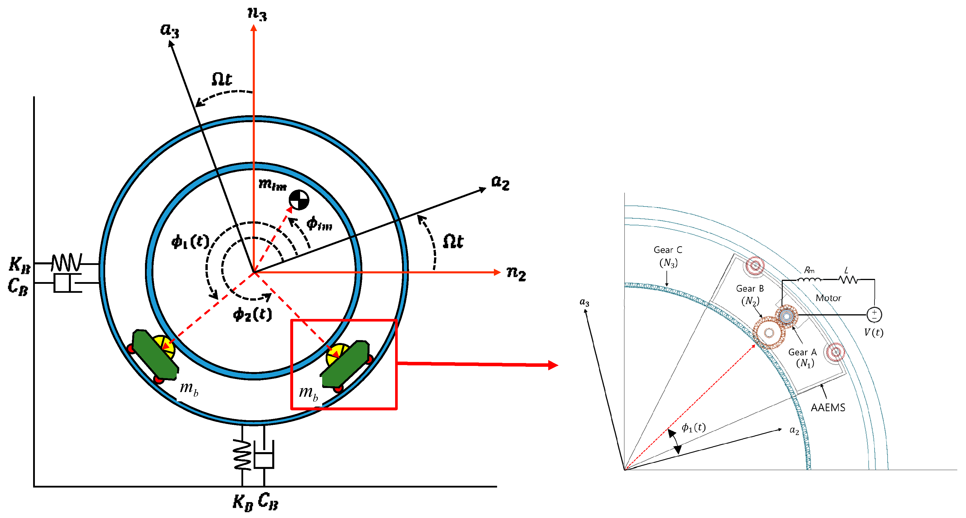
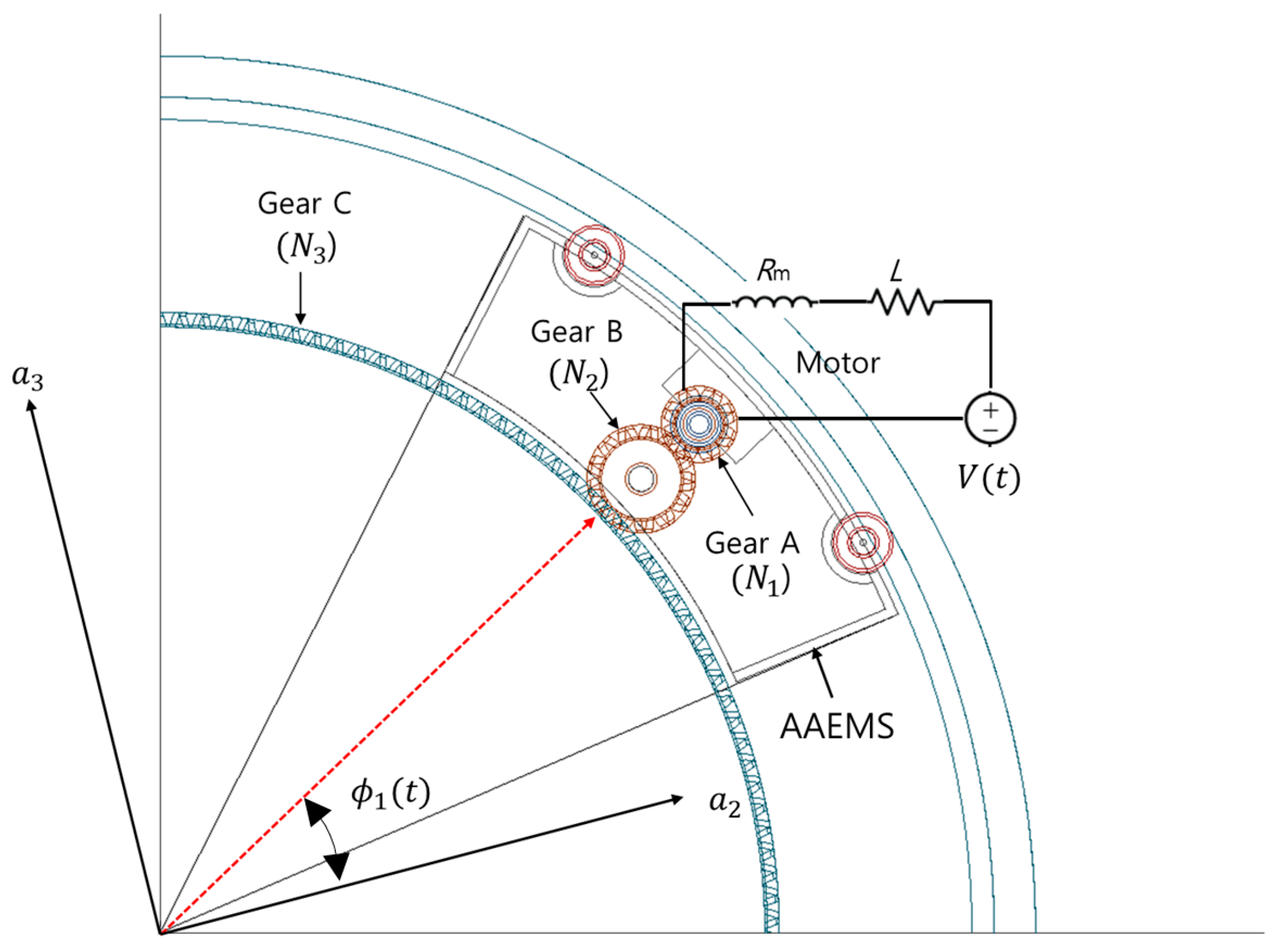
This section presents the model of the imbalance rigid planar rotor system equipped with dual AAEMS supported by a normal symmetric passive bearing as described in Figure 1. Here, the AAEMS can be mobilized via its own actuating capability inside of a circular guided track, which is specified by a circular static gear C (N3) and synchronized with rotating speed. The motor inside AAEMS conveys a torque to gears A and B so that AAEMS marches on the static gear C contacted by the gear B. Since the system is assumed to be mounted on a symmetric passive bearing, the equation of motion and the control design of the AAEMS for the proposed system has been conducted with respect to the rotor fixed frame instead of the fixed frame .
Considering the horizontal and vertical displacement of the rotor together with the angular positions of AAEMS as the states of system such that referenced to , the equations of motions is given by
where, , and are the mass, damping, and stiffness matrices of proposed system, respectively, and they are provided by
where, , , and are the mass of the rotor, the mass of an AAEMS and the radius of a circular guided track, respectively. Moreover, and are constant damping and stiffness coefficients of linear bearing. In addition, , (for i = 1,2) and are the force vector due to imbalance, the force vector via AAEMS as well as the force vector due to the coulomb friction between the contact surfaces of AAEMS and the circular track’s and given by
where, , and are the static equivalent imbalance mass, the radial location of the mass, and its angular phase. Moreover, the coefficient is the constant rolling coefficient of coulomb friction. It is assumed that the viscous damping of AAEMS is negligible due to the constraint that the moving speed of AAEMS is limited.
Additionally, the matrix in (1) is an adjusting matrix and the vector in (1) represents the actuating torques of AAEMS, and those details are provided by
To develop the further estimation and control strategies, it is convenient to partition the original dynamics (1) into two parts, the unactuated and actuated states of system:
where, and are an un-controlled state vector and a controlled one, respectively.
Consequently, the force vectors in the right side of (1) are accommodated as follows:
Specifically, another form of (7) is followed as
Furthermore, the relation between the control voltage of the motor and the torques of AAEMS in (6) is given by
The detail of the derivation of (10) is presented in the Appendix A.
Using (10), the second equation in (9) can be adopted as follows:
The first equation in (9) and (11) will be used throughout the paper to develop the estimation and control strategies.
3. AAEMS-Based Imbalance Vibration Control Strategy
The novel control strategy using dual AAEMS moving around a circular guided track has been described here to provide the possibly complete suppression of imbalance vibration for a rotating rotor.
Unlike a passive automatic balancing device (ABD), the AAEMS is a motorized eccentric mass so it can autonomously reach any angular position of a circular guided track attached to a rotating imbalanced rotor. Therefore, this AAEMS is capable of generating any directional counter effective centrifugal force against any random static rotor imbalance. In other words, once the magnitude and the angular position of the imbalance are identified, this actively controlled system can be dispatched to the desired angular position where the effective imbalance force is completely or partially eliminated. It is very powerful and a direct approach to deal with the imbalance vibration in the rotor system and possibly anticipated to achieve “literally the zero level of imbalance vibration”.
To guarantee such an autonomous performance of AAEMS, the control strategy proposed here is equipped with the following primary functions.
- (A)
- First, it is necessary to identify the rotor imbalance and the resistive frictional force acting on the AAEMS to facilitate the control of the AAEMS. Therefore, two Kalman Filters are employed to sequentially estimate the unknown imbalance of the rotor (i.e., , and ) and the coefficient of coulomb friction between the contact surface of the circular track (i.e., Gear C) and the counter-contacted parts (i.e., Gear B) of AAEMS. Here, during the imbalance estimation, two AAEMSs were arranged to be maintained for each other in 180 degrees angular phase and synchronized with a rotating rotor (i.e., not under any motion relative to the rotor). Thus, the centrifugal force via the first AAEMS cancels the second one, resulting in no effect of AAEMS in the system during the imbalance estimation. After that, the estimation of the unknown coulomb friction coefficient for each AAEMS was conducted while both AAEMSs were enforced to be circulated around together with a constant speed maintaining each other in a 180 degrees angular phase. This way can minimize the perturbation of the system as well as possibly reduce the error of estimation. These two estimations are explained in the Section 3.1 (imbalance estimation via Kalman filter) and Section 3.4 (friction coefficient estimation via extended Kalman filter), respectively.
- (B)
- Based on the estimated imbalance in (A), the desired angular positions of both AAEMSs can be determined using the condition, (from the right side of the 1st equation in (9)). Then, the minimum travel between the initial angular positions of AAEMS and the desired angular ones is identified by computing all the possible traveling distances from the current positions of the AAEMS to the desired ones. These can be found from Section 3.2 and Section 3.3.
- (C)
- Subsequently, the angular position controls of both AAEMSs were executed based on the desired angles of AAEMS determined in (B). Here, an LQR-based optimal control was applied, which conducted the angular position control of both AAEMSs and reduced the control power consumption of the actuators in AAEMSs. Additionally, it should be stated that this position control also incorporates with the compensation of disturbing force due to coulomb friction using the estimates obtained in (A). The details of this control are presented in Section 3.5.
- (D)
- The sequential estimation and control processes proposed in (A) through (C) may not exhibit the desirable performance under the situation where the estimation errors and intolerable disturbances are presented. Thus, the trial–error-based fine-tuning angular position control for AAEMS was accompanied with it as the last line of defense for the further imbalance suppression. The details of this approach are described in Section 3.6.
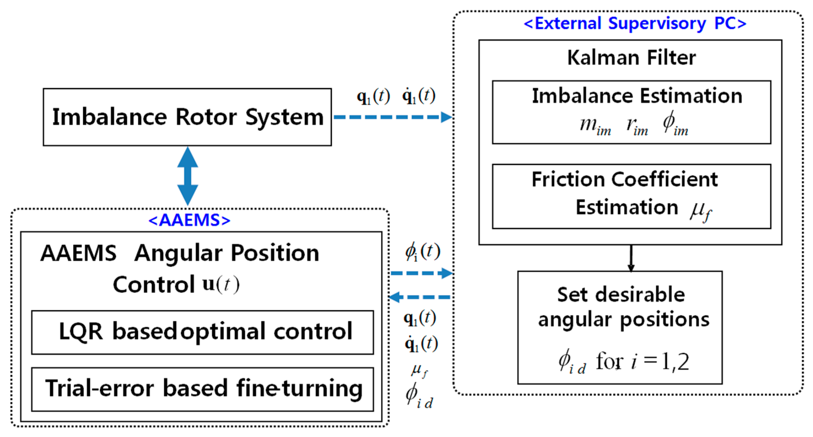
Based on (A), (B), (C) and (D) above, Figure 2 briefly outlines the entire scheme of AAEMS-based imbalance vibration control.
Also, before proceeding further, the following assumptions were made.
- (I)
- It is assumed that the sensors (i.e., a laser-based sensor or an accelerometer) constantly monitors the transversal amplitudes and velocities of the rotor (i.e., and ).
- (II)
- Each AAEMS consists of a geared motor, a small-sized encoder, its own micro controller unit together with a motor driver, as well as a rechargeable mini NiMH battery. In the sense that the wide application of a small drone dramatically reduces the weight and size for both battery and its compatible powerful motor, such a compact arrangement has recently become attainable.
- (III)
- The angular positions of the AAEMS for i = 1,2 are measured by a rotary encoder installed in themselves and both and can be obtained based on the together with a proper sampling time.
- (IV)
- An external supervisory PC wirelessly communicates with the micro-controller unit in each AAEMS. Thus, for the angular position control, AAEMS sends its own angular position to PC and receives the motions and rotating speed of the rotor.
3.1. Unknown Imbalance Estimation
During the imbalance estimation, it was enforced that both the AAEMSs were arranged to be halted for each other in a 180 degrees angular phase. This means that , (for i = 1,2) as well as .
Therefore, the dynamic forces generated by AAEMS are disregarded so that the components representing any motions of AAEMS in the system are no longer effective and in (9) due to the condition .
Consequently, the first equation in (9) simply results in the linear baseline system w/o AAEMS and given by
where,
,
, and,
.
Let us define the estimates of rotor imbalance as a vector: .
Furthermore, the linear dynamic system in (12) can be placed into the first order form:
For the estimation of via Kalman filter [25], (13) is discretized and it is followed by:
where, is a sampling time and the sub-notations k-1 and k indicate the previous time and the current one, respectively. Additionally, is the estimate vector at the previous time k-1 and is the estimate vector predicted at time k. Based on the previous estimates , the predicted estimates are obtained through a transition matrix .
The predicted error covariance at time k was predicted by the previous error covariance :
where, for i = 1,2,…,6 is the covariance of the process noise. Here, the randn represents a function generating uniformly distributed random real numbers.
The innovation of Kalman filter (KF) is given by
where:
The vector is obtained by a sensor. Furthermore, the optimal Kalman gain is computed by
where, .
The covariance of the observation noise, is:
Finally, the predicted state estimate in (12) is updated by
Moreover, the predicted error covariance is updated by
where, is an identity matrix.
From the estimates in for , the unknown imbalance can be identified:
Furthermore, the magnitude and angular phase of imbalance can be obtained by
The results in (23) can be used for the determination of desired angular positions of AAEMS.
3.2. Desired Angular Positions of AAEMS
Then, the desired angular position of each AAEMS was considered for the estimated imbalance in (23). Based on (8) and (9), to achieve the zero force excitation in an imbalance rotor system, the following condition should be met:
The desired steady-state angular positions of AAEMS can be inferred from (24).
With condition for i = 1,2, (24) becomes:
Solving (25) for and yields the target angular positions of AAEMS:
where is the arc-length of the center-line for an AAEMS. (26) describes the two cases: the first one indicates the complete cancellation of imbalance for the case that the imbalance force is less than the static centrifugal force due to AAEMS while the second one refers to the maximum allowable suppression that the AAEMS can generate (where the imbalance force is greater than the force due to the AAEMS).
3.3. Minimum Travel Plan of AAEMS
After determining the desired angular positions of the AAEMS (i.e., and in (26)) to achieve the statically balancing condition in the rotating rotor system, it is necessary to efficiently allocate and to each AAEMS, because the travel distance of each AAEMS must be minimized to reduce the actuating power consumption of the AAEMS together, with less perturbation of the system. To achieve such efficient implementation, one may see the two possible cases:
where is the travel distance between the current angular positions of AAEMS, and .
Then, a particular case indicating the minimum distance between the first equation and the second equation was simply chosen in (27):
According to (26), if , enforce that and . Otherwise, and . This strategy also prevents the collision between two AAEMSs operating in the same circular track and this plan will be used in the angular position control of AAEMS, shortly introduced in Section 3.5.
3.4. Estimation Of Coulomb Friction
To implement the accurate position control of AAEMS, this system should consider the friction force between the contact surface of the circular track and the counter-contacting parts of the AAEMS and it is clearly advantageous to eliminate this disturbing force. As shown in (5b), the coulomb friction can be found if the friction coefficient is identified. Therefore, this Section presents the estimation strategy of by operating an additional extended Kalman filter [25]. The estimation strategy is enforced in the way that both AAEMSs are simultaneously moving around the circular track with identically regulated constant speeds maintaining each other in a 180 degrees angular phase. Such an approach enabled us to not only estimate but also minimize perturbing the entire system during the estimation period because the centrifugal force due to the first AAEMS eliminates the second’s.
For the estimation of , revisiting to the second equation in (9):
Based on (29), proposing the control law to actuate both the AAEMS around the circular track in constant speeds as identical as possible such that:
The part (a) in (30) eliminates the disturbing terms which can be computed via the known system parameters and the sensor values while in part (b) in (30), , induces both AAEMSs being rotated at an identical constant speed, . In addition, is a constant positive control gain.
Applying (30) into (29) and rearranging it results in:
Let the estimates for the friction coefficient be a vector: .
Discretizing both (31) and (an unknown constant vector) using the sub-notations k − 1 (previous time) and k (current time):
where and is a sampling time.
Introducing the coordinates of the estimates (i.e., the predicted state vector) and (i.e., the previous state vector), the linearized prediction model for extended Kalman filter can be provided by
where is Jacobian.
The detail of Jacobian in (33) is followed by
where:
Here, for i = 1,2 shown above represents the Dirac delta function.
Due to the derivatives of with respect to for i = 1,2, it is inevitable to avoid the Dirac delta function thus the following approximation is used for :
where a is the constant and selected as 0.05.
Similarly, as done in the Section 3.1, the predicted error covariance at k-th time is predicted by the previous error covariance :
where for i = 1,2,3,4 is the covariance of the process noise.
The innovation of EKF is given by
where which can be measured by the sensors (i.e., a rotary encoder in AAEMS) and .
The optimal Kalman gain is obtained by
where, is the covariance of the observation noise.
The state estimate is updated by and the predicted error covariance is updated by .
The stability of the entire system should be investigated for the effect of estimation strategies, because both AAEMSs are moving around the rotating rotor and then may affect the stability of the rotor.
Therefore, the stability of the rotor was explored based on Lyapunov stability. It was found that the motion of rotor is ultimately bounded under the condition that the damping of the bearing is sufficiently large to endure the perturbation via AAEMS. The detail of proof is presented in the Appendix B.
3.5. LQR Based Angular Position Control of AAEMS
For the control of the angular position for AAEMS based on the second equation in (9), proposing the control law such that:
where .
The control law consists of three parts. The first and second parts referred to (a) and (b) above cancel the non-linear term of (9) and the friction effect of AAEMS. An additional term (c) indicates the angular position control of AAEMS.
Applying (39) into the second equation in (9) yields:
Now, we need to design such that (40) reaches the following invariant set :
where, indicates the target angular positions of both AAEMSs, which are determined by (25) and (26).
Defining and then placing (40) into the first order form:
where, , and .
The control input is determined by minimizing the following cost function:
where, and are symmetric positive definitive.
Defining Hamiltonian:
where, is a Lagrangian multiplier.
The solution of (44) is well known and can be obtained by
Together with (42), from (45) and (46):
The matrix can be obtained by Algebraic Riccatti equation as shown below:
Finally, the optimal control law can be found:
where, .
Based on (49), (40) is globally exponentially stable at the desired equilibriums shown in (41).
Furthermore, due to the action of resulting , the first equation in (9) is turned into:
Equation (50) implies that the imbalance rotor system is globally asymptotically stable at the origin (i.e., , , and ).
3.6. Fine-Tuning-Based Angular Position Control of AAEMs
Although the position of AAEMS is controlled via the law in (39), the most minimal vibration level may not be achieved under the presence of estimation errors and unpredictable disturbances.
Therefore, the trial–error-based fine-tuning angular position control of AAEMS was addressed to resolve this challenge. In order to minimize the remaining vibration level of the rotor system, the following objective function is proposed, which represents the integral of the vibration amplitude over a certain period of time [,]:
Expressing (49) in the discretized manner yields:
where n is the number of segments for the time range [,] and .
To find the particular and , minimizing (52) via the trial–error approach, (52) is evaluated for the four small perturbation of specified below:
where, indicates the small perturbation of both AAEMSs in the counter clockwise direction while perturbs the first AAEMS in the clockwise direction and the second one in the counter clockwise direction.
Moreover, the action stimulates both AAEMS in the clockwise direction. On the other hand, refers to a small perturbation of the first one in the counter clockwise and the second one in the clockwise direction.
Then, let us find the minimum among the four cases below:
By doing the processes (53) and (54) recursively and continuously, the most minimum can be possibly found.
Under the presence of the unavoidable errors and disturbances in the process of estimations and controls, the fine-tuning approach introduced here should be accompanied together with (39) to accomplish the acceptable imbalance vibration, such as . Therefore, this trial–error-based fine-tuning angular position control of AAEMS is the ultimate defense of the system against imbalance vibration.
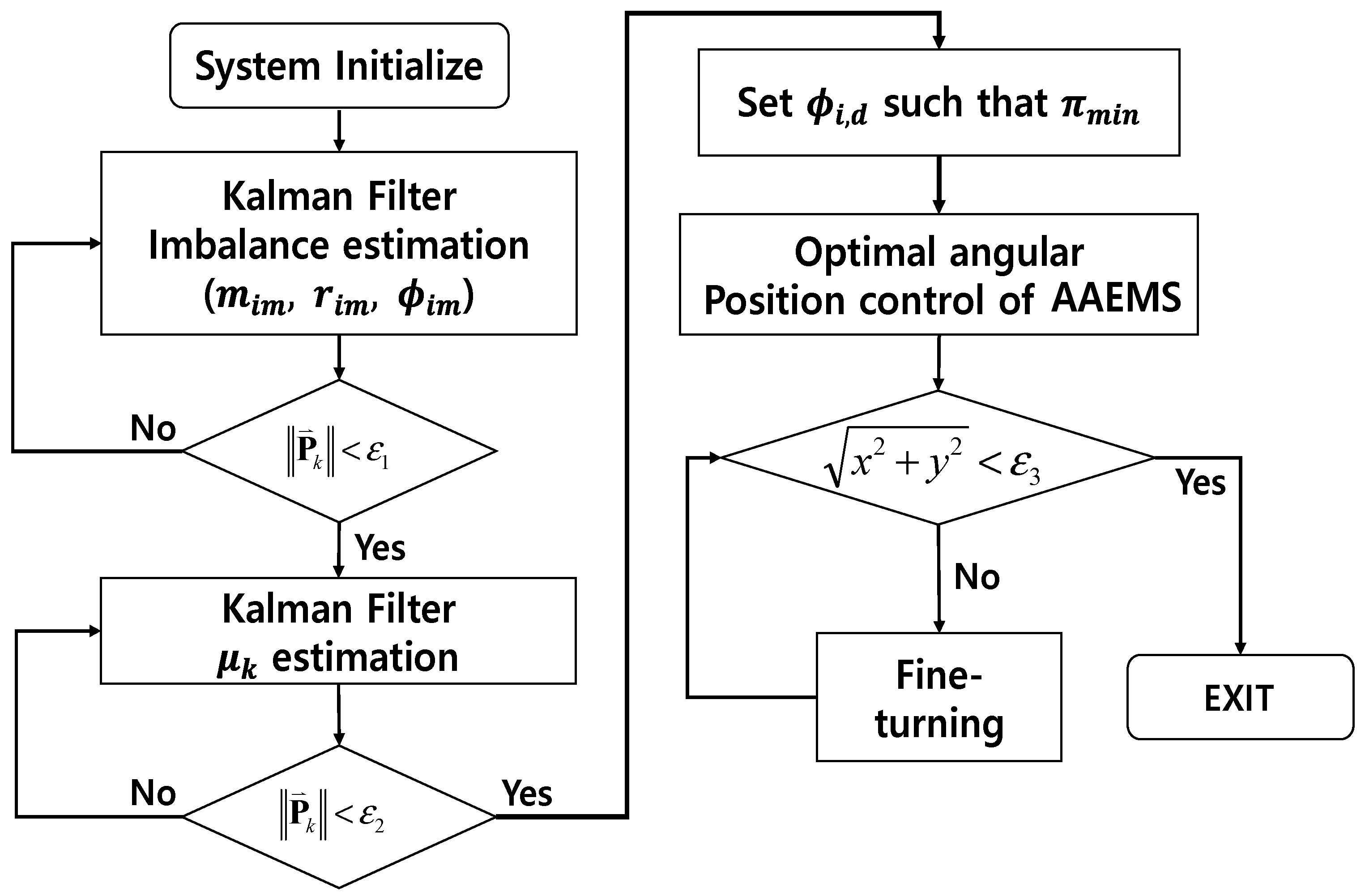
Figure 3 describes the entire control flow of AAEMS. First, a Kalman filter estimates the imbalance of the rotor and then another Kalman filter identifies the friction coefficients of the contacted parts in AAEMS. Both estimations contain the monitoring processes to check the conditions that the error covariances are sufficiently small (i.e., and ). In the next step, the target angular positions of the AAEMS are determined based on the estimated imbalance and an efficient allocation of both AAEMS for is performed to achieve the minimum travels of both AAEMSs. The angular position control of the AAEMSs is followed. Once the angular position control is successfully completed, no further control is required (i.e., ). Otherwise, the fine-tuning control is activated for the further regulation of imbalance vibration.
4. Simulation Results
To explore the effectiveness of the proposed AAEMS system for imbalance vibration control, the simulations were conducted in this section.
The parameters of the system for the subsequent simulation are shown in Table 1 and are utilized throughout the paper, unless specified otherwise.
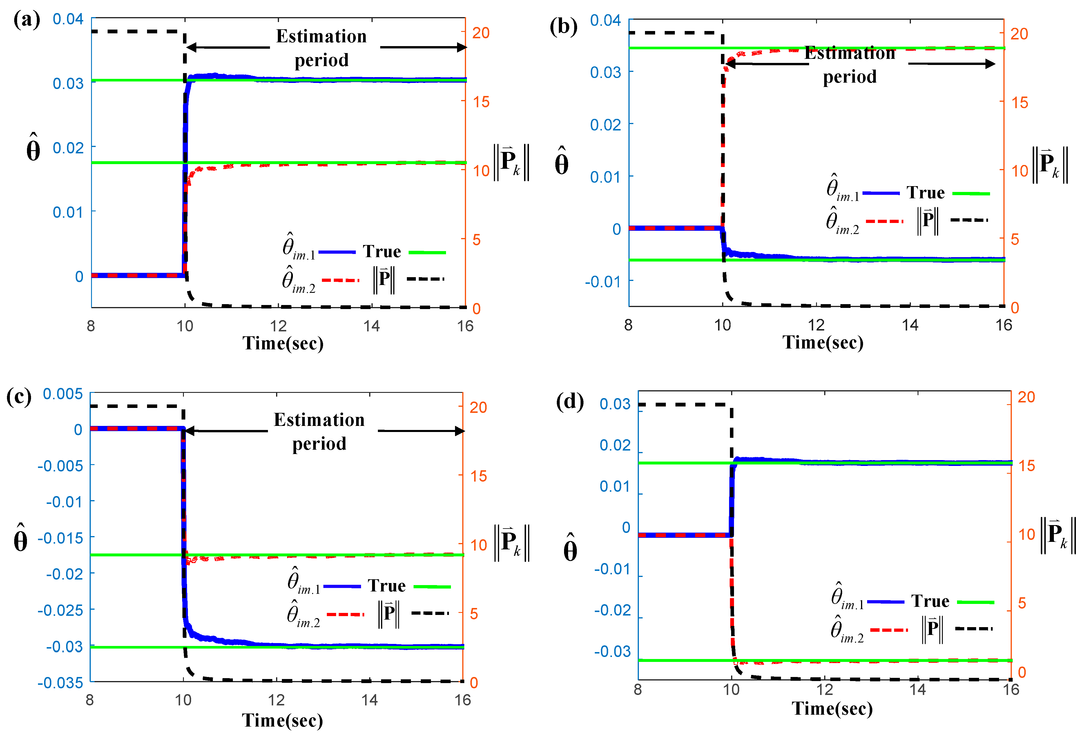
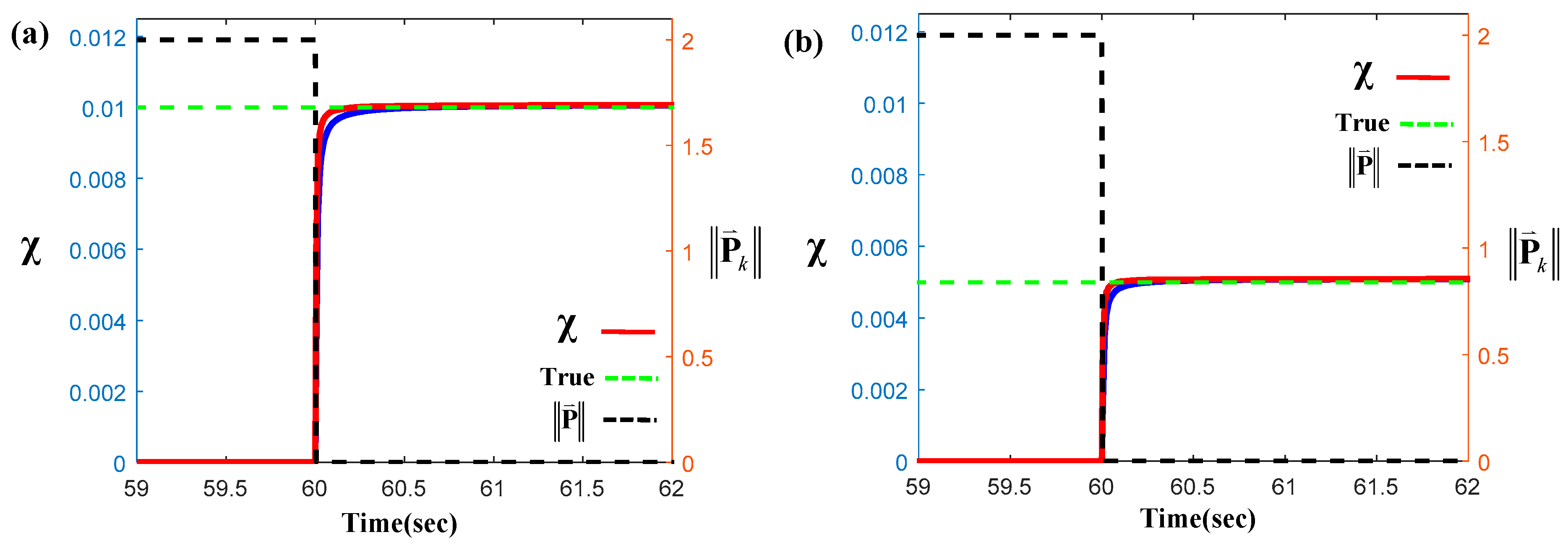
Figure 4 shows the estimates of four different imbalance cases to assess the strategy in Section 3.1. The angular phases of imbalance employed in (a), (b), (c) and (d) of Figure 4 were 30, 100, 210, and 300 degrees, respectively. Each result contains imbalance estimates and the norm of covariance represents the error magnitude between the estimates and the assumed actual ones. It was found that the final estimates were well synchronized with the true values and the norm of in each case was converged to zero. Moreover, all the results show that the estimates approach to the true ones within approximately 3~4 s, after the estimation is initiated. The strategy of imbalance estimation proposed here provides unknown imbalance accurately and quickly.
On the other hand, Figure 5 presents the estimates of the assumed friction coefficient between the surfaces of the circular track and the counter-contacted parts of AAEMS. Here, it is assumed that each friction coefficient is identical for each other (i.e., ). As shown in Figure 5, it was discovered that the estimates were well matched with the assumed true ones and the norm of became sufficiently small as a time marched forward. This indicates that the estimation approach presented in Section 3.4 also demonstrates quick and precise estimation performance.
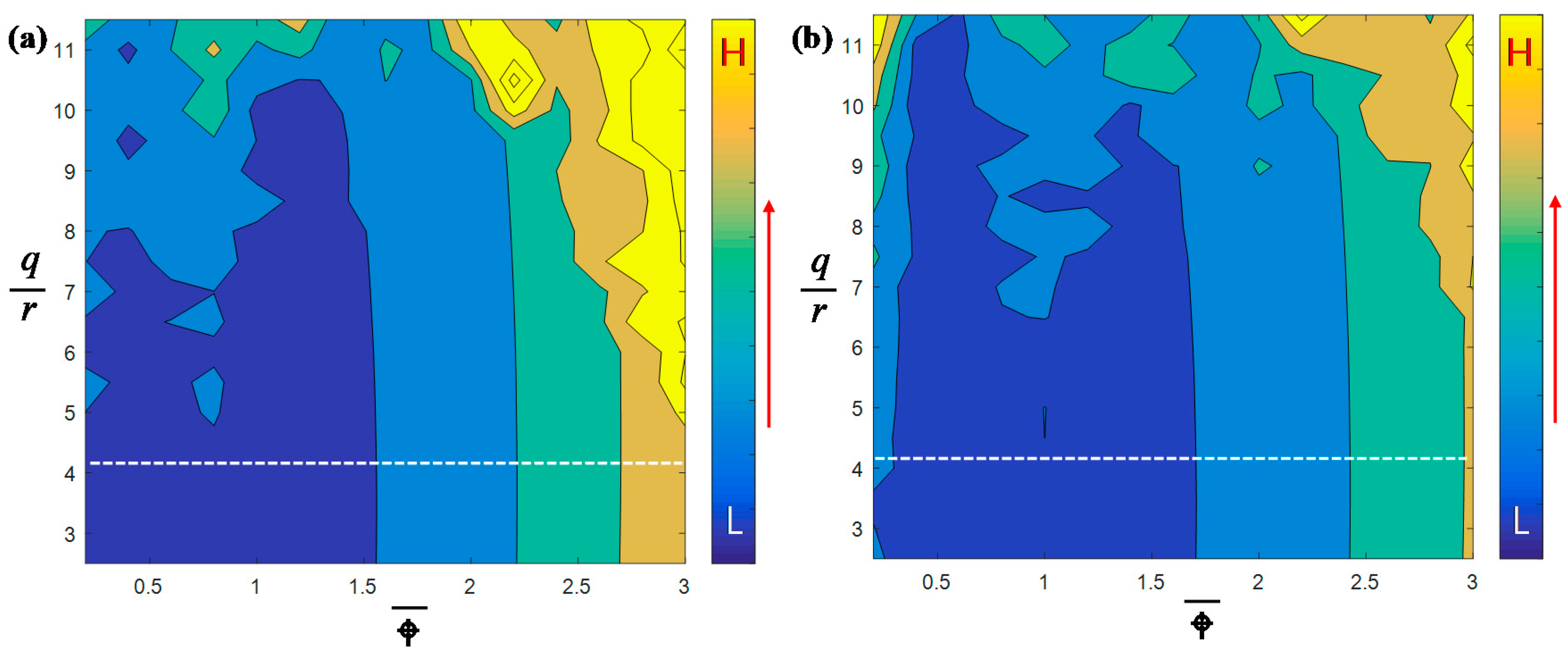
Figure 6 indicates the consumption of control force (given by (55)) integrated over a time from to for the parameters (q, r) and non-dimensional rotor rotational speed . Here, the q and r are the scalar weight parameters for the matrices and in (43). It should be noted that = q [0.1 0 0 0; 0 0.1 0 0; 0 0 0.01 0; 0 0 0 0.01] and = r [0.1 0;0 0.1] were chosen here. Moreover, and are the initial time and the time that the control in (39) is terminated, respectively. Figure 6a shows the result for the case (mass ratio) and Figure 6b describes the outcomes for . It is found from Figure 6 that the index in (55) increases as the rotational speed does. As the ratio increases, it is obvious that is augmented. Based on the results in Figure 6, the reasonable ratio can be determined as between 3 and 4 thus in (49) was obtained via this guideline. Additionally, as the ratio is increased, we can observe that tends to be greater for the same and :
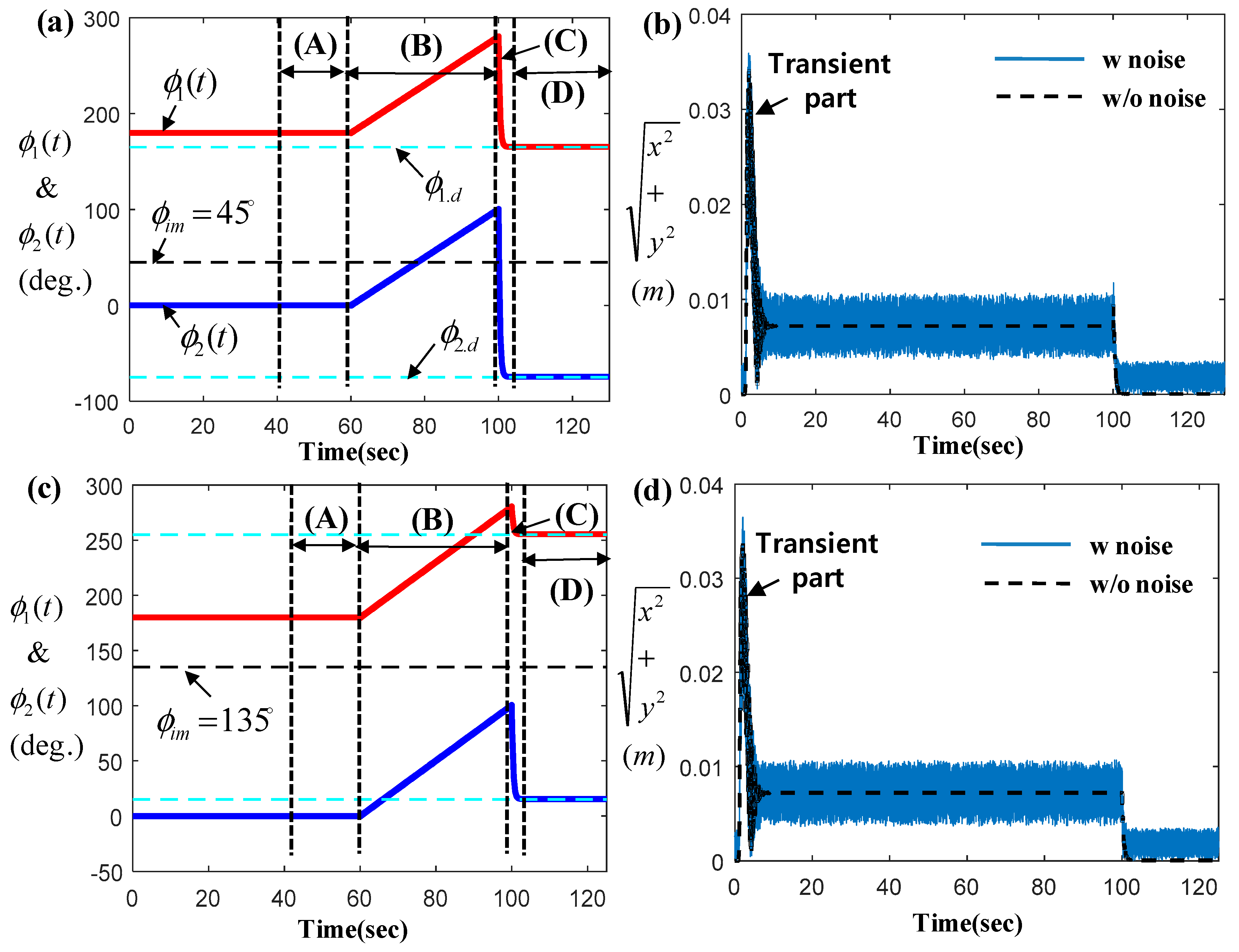
For two different imbalance cases, Figure 7 shows the controlled angular coordinates of AAEMS and the corresponding vibration amplitudes on the time domain. (a) and (b) of Figure 7 represent the results for while (c) and (d) contain the outcomes for . In addition, the periods specified via (A), (B), (C) and (D) in (a) and (c) of Figure 7 are described below:
- (i)
- Period (A): Imbalance estimation in Section 3.1 was performed under the condition that both AAEMSs remained halted and were initially assigned a 180 degrees angular phase difference for each other.
- (ii)
- Period (B): According to the Section 3.4, the friction coefficients were estimated while moving two AAEMS simultaneously with an identical constant speed maintaining a 180 degrees angular phase for each other.
- (iii)
- Period (C): The angular positions of both AAEMSs were controlled via the LQR-based optimal control presented in Section 3.5. Here, it should be mentioned that the determination of the desired angular positions for an estimated imbalance (in the Section 3.2) and the minimum travel based efficient assignment of AAEMS (presented in the Section 3.3) were conducted prior to this control period.
- (iv)
- Period (D): Once both AAEMSs reached the target angular positions, the two AAEMSs were no longer actuated.
It should be mentioned that each period above can be intentionally reduced by manipulating the estimation and control parameters.
As seen from (b) and (d) of Figure 7, the vibration amplitudes of the rotor corresponding to the periods (A) and (B) were not perturbed due to the estimation strategies presented in Section 3.1 and Section 3.4 On the other hand, it can be seen from the periods (C) and (D) that the amplitudes have been decreased and almost reached zeros via the control of AAEMS. Additionally, due to adaptive filter-based estimations, it should be emphasized that all the functions of AAEMS properly work, even under the presence of assumed artificial noise in rotor vibration. Therefore, by investigating the results in Figure 7, the performance of AAEMS can be guaranteed as long as the estimation errors are not presented.
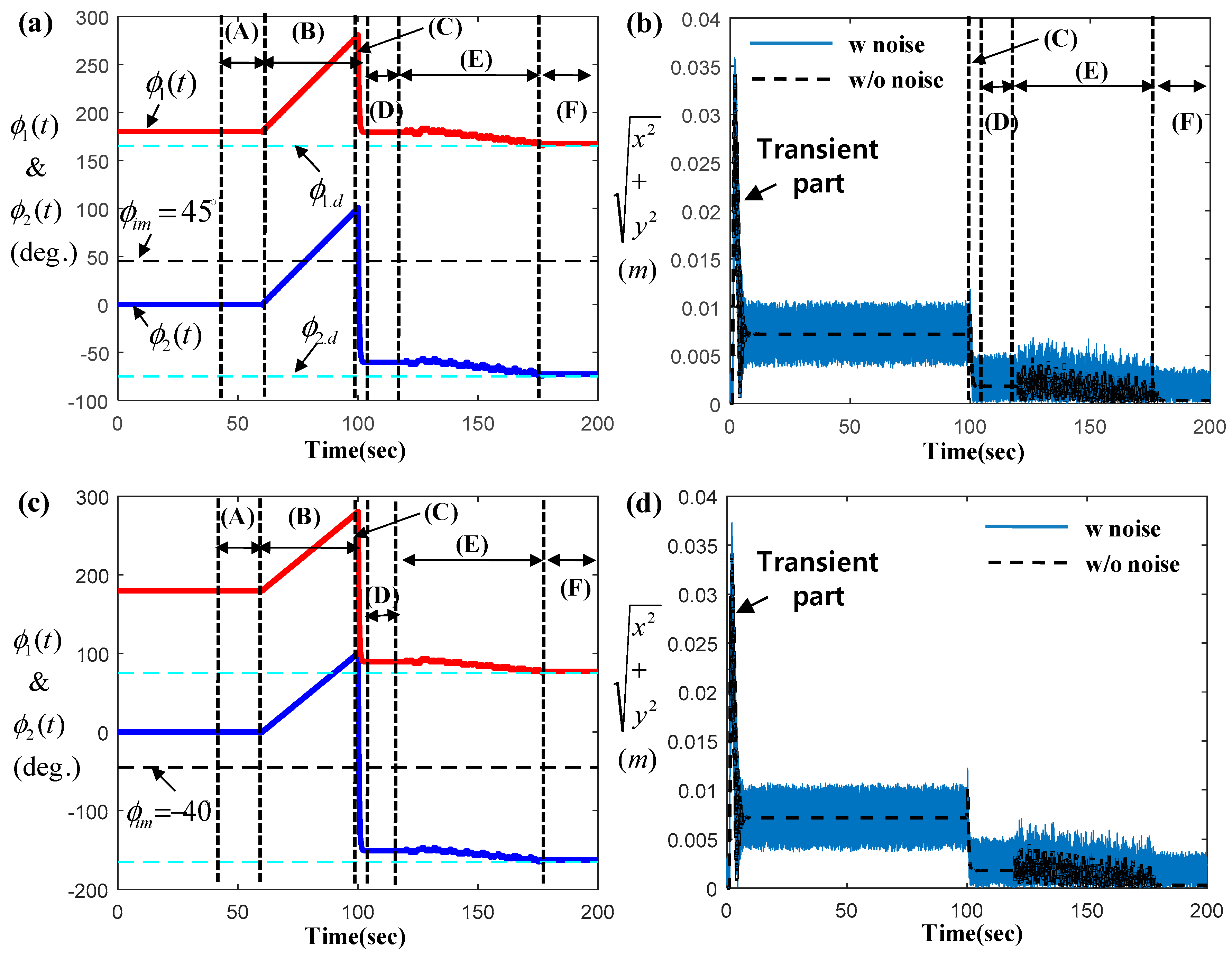
Figure 7 discusses some ideal situations with perfect estimations and control. However, there will be unavoidable errors and disturbances in both estimations and controls for actual applications. Therefore, the trial–error-based fine-tuning control of AAEMS was discussed in Section 3.6 to supply an additional counter-measure for an unacceptable vibration amplitude for unexpected events. Figure 8 simulates the condition where the estimation error is intentionally assumed to be presented, thus it can be seen that both AAEMS do not reach the most advantageous position for imbalance vibration control. Therefore, it was observed from the periods (D) in both (a) and (c) of Figure 7 that the relative deviations of the angular position between AAEMS and the target positions are not negligible and the deviations are approximately 10 degrees. Consequently, the corresponding vibration amplitudes shown in periods (D) in both (b) and (d) of Figure 8 are not sufficiently small.
Therefore, the fine-tuning position control was initiated during the period (E) as shown in both (a) and (c) of Figure 8. Due to this additional action, we can find from the periods (E) and (F) in (b) and (d) of Figure 8 that the vibration amplitudes undergo radical change but finally reach the acceptable level of vibrations.
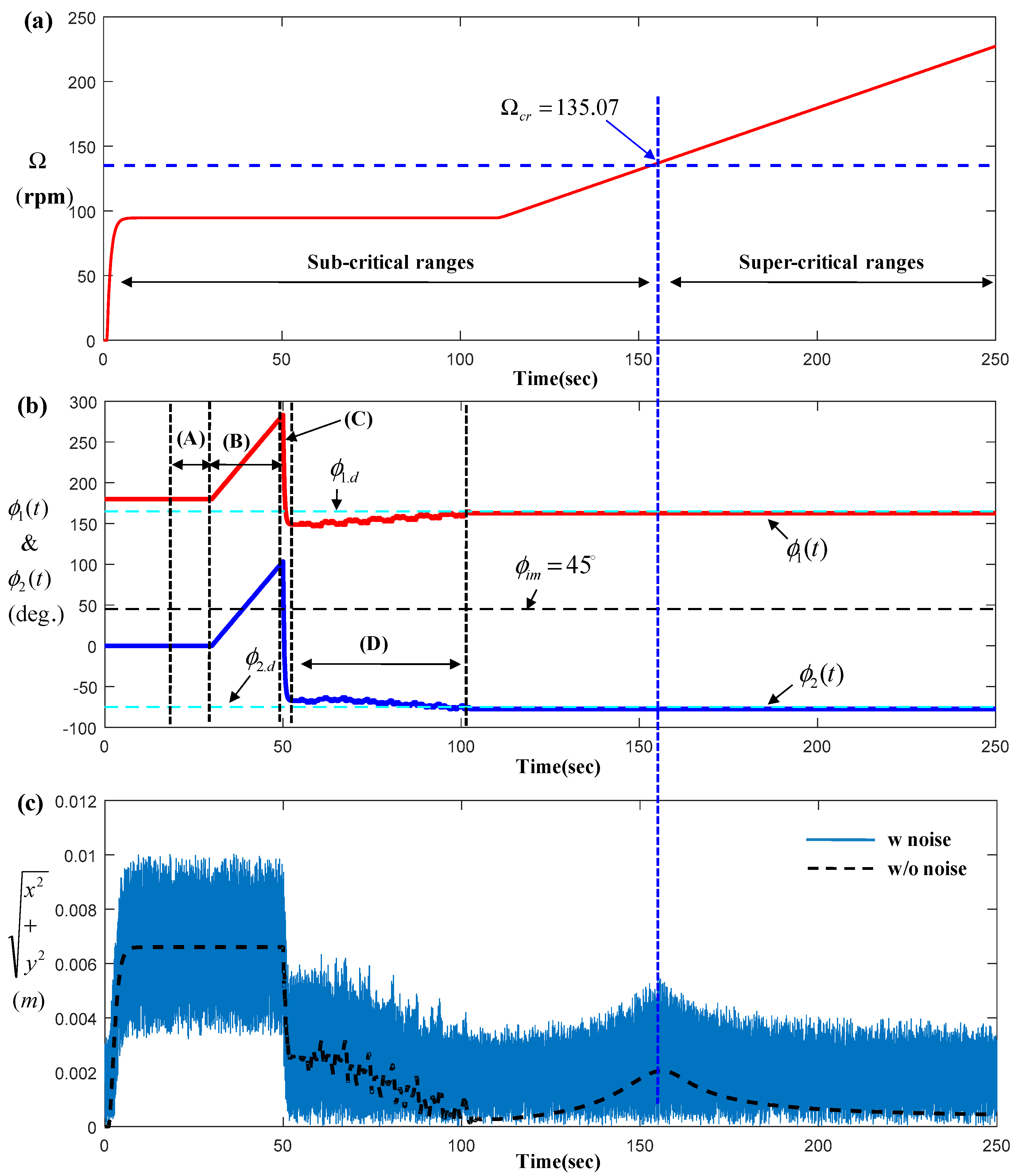
Figure 9 simulates a particular scenario that demonstrates the more powerful effectiveness of the proposed AAEMS. The outcomes in (a), (b) and (c) of Figure 9 indicate the profile of the rotating speed of the rotor, the angular positions of the two AAEMS as well as the corresponding vibration amplitudes of the rotor on the time domain, respectively. As seen from the results of Figure 9, the estimations and controls were executed at the low constant operating speed, approximately 100 rpm and then the rotor speed was linearly increased up to 230 rpm. Due to the acceleration of the rotor, the entire system must experience a critical speed rpm, with a slight oscillation amplitude near 155 s, as shown in (c) of Figure 9. However, it is clear that the vibration amplitude was not seriously significant, even at the critical speed since the imbalance force has been already attenuated by the action of AAEMS at the sub-critical speed (i.e., below a critical speed). The control scenario shown in Figure 9 is especially applicable to the vibration control of washing machines which have to pass through the critical speed because they should be operated at both the sub-critical speeds (for a washing process) and the supercritical ones (for a dewatering process).
5. Conclusions
This paper proposed a new control strategy for a novel AAEMS for cancelling the rotor imbalance vibration. Due to the adaptive estimations and efficient controls, this approach can achieve the nearly zero-imbalance vibration of a rotor, even under the presence of assumed artificial disturbances and errors. To achieve such excellent performance, three primary functions of AAEMS were proposed in this study.
(i) First, two Kalman filters were employed to sequentially estimate the unknown imbalance of the rotor and the disturbing force due to coulomb friction of AAEMS. (ii) Second, the efficient angular position control of the AAEMS by using an LQR-based optimal control that simultaneously minimizes the imbalance vibration of the rotor and the power consumption of the AAEMS actuator was presented. (iii) Third, the trial–error-based fine-tuning angular position control was equipped with the AAEMS for the additional imbalance suppression under the situation where the estimation errors and disturbances are presented.
The simulation results demonstrate the effectiveness of control strategy for the AAEMS system. The control strategy in this paper provides important insights for the researchers wishing to utilize the direct automatic balancing of imbalance rotor. The next study will include the validation of proposed control system via an experimental set-up. Besides the control strategy for AAEMS, this study also provides the useful holistic reviews of the imbalance vibration control and the isolation-based ABD, AMB, as well as other approaches.
Funding
This work was funded by the KETEP as Human Resources Development Programs (Grant No. 20194010201800).
Acknowledgments
This work was supported by the KETEP as Human Resources Development Programs (Grant No. 20194010201800) and supported by the KETEP and the MOTIE of the Republic of Korea (No.20194030202300).
Conflicts of Interest
The authors declare no conflict of interest.
Appendix A
Figure A1.
re-captured image of AAEMS from Figure 1.
Figure A1.
re-captured image of AAEMS from Figure 1.

The dynamics of the electrical motor inside of an AAEMS is provided by
where , , , , and are the motor resistance, current, inductance, EMF, and control voltage, respectively. In addition, , , , , and are the motor–gear inertia, a viscous damping ratio, a rotational angular position of motor shaft, a motor constant, and a load torque induced by B gear, respectively.
Since and it is assumed that the effect of L is insignificant, (A1) becomes:
(A2) and (A3) yields:
The dynamics of B gear is given by
where , , , , and are the B gear inertia, a viscous damping ratio, a rotational angular position of B gear, a conveyed torque from a motor and a load torque induced by C gear, respectively.
Applying and into (A5) yields:
where is a gear ratio between A gear and B gear.
From (A4) and (A6):
Applying and creates:
Under the assumption that is sufficiently small:
Considering two of (A9) (i.e., ):
where:
and
Appendix B
The stability of the rotor system was discussed in Section 3.4. Let us consider the first equation in (9) with respect to the fixed frame instead of the rotor-fixed frame . Therefore, applying the transformation matrix into the first equation in (9) yields:
where , , , [ ; ], [ ; ],
Now, we have the E.O.M of (9) with respect to . Additionally, it should be noted that the transversal displacement of a rotor is expressed with respect to (i.e., ) but the angular coordinates of AAEMS are still measured relative to the frame .
Then, let the candidate Lyapunov function be:
Taking a derivative of V(t) with respect to a time and then substituting (A11) into yield:
Furthermore, taking the norm of all vectors and matrices in (A13) yields:
Since the following norms , ,, and are bounded, ( and are regulated by the control law in (30), resulting in being bounded), we can find a constant Y such that:
From (A14), it can be seen that . This implies that is ultimately bounded. Under the condition , it is seen that , leading to the fact that is also bounded. Consequently, is bounded either.
References
- Lum, K.Y.; Coppola, V.T.; Bernstein, D.S. Adaptive Autocentering Control for an Active Magnetic Bearing Supporting a Rotor with Unknown Mass Imbalance. IEEE Trans. Control. Syst. Technol. 1996, 4, 587–597. [Google Scholar] [CrossRef] [Green Version]
- Sun, L.; Krodkiewski, J.M.; Cen, Y. Self-Tuning Adaptive Control of Forced Vibration in Rotor Systems Using an Active Journal Bearing. J. Sound Vib. 1998, 213, 1–14. [Google Scholar]
- Zhou, S.; Shi, J. Active Balancing and Vibration Control of Rotating Machinery: A Survey. Shock Vib. Dig. 2001, 33, 361–371. [Google Scholar] [CrossRef] [Green Version]
- Desmidt, H.A.; Wang, K.W.; Smith, E.C.; Provenza, A.J. On the Robust Stability of Segmented Driveshafts with Active Magnetic Bearing Control. J. Vib. Control 2005, 11, 317–329. [Google Scholar] [CrossRef]
- Kang, H.; Oh, S.Y.; Song, O. H control of a rotor-magnetic bearing system based on linear matrix inequalities. J. Vib. Control 2001, 17, 291–300. [Google Scholar]
- Fang, J.; Xu, X.; Xie, J. Active vibration control of rotor imbalance in active magnetic bearing systems. J. Vib. Control 2005, 21, 684–700. [Google Scholar] [CrossRef]
- Thearle, E.L. Automatic dynamic balancers (Part 2-Ring, pendulum, ball balancers). Mach. Des. 1950, 22, 103–106. [Google Scholar]
- Kubo, S.; Jinouchi, Y.; Araki, Y.; Inoue, J. Automatic balancer (pendulum balancer). Bull. JSME 1986, 29, 924–928. [Google Scholar]
- Bovik, P.; Hogfords, C. Autobalancing of rotors. J. Sound Vib. 1986, 111, 429–440. [Google Scholar] [CrossRef]
- Majewski, T. Position error occurrence in self balancers used on rigid rotors of rotating machinery. Mech. Mach. Theory 1998, 23, 71–78. [Google Scholar]
- Jinnouchi, Y.; Araki, Y.; Inoue, J.; Ohtsuka, Y.; Tan, C. Automatic balancer (static balancing and transient response of of a multi-ball balancer). Trans. Jpn. Soc. Mech. Eng. 1993, 59, 79–84. [Google Scholar] [CrossRef] [Green Version]
- Lindell, H. Vibration reduction on Hand-Held Grinders by Automatic Blancers. Cent. Eur. J. Public Health 1996, 4, 43–45. [Google Scholar] [PubMed]
- Rajalingham, C.; Bhat, R.B. Complete Balancing of a disk Mounted on Vertical Cantilever Shaft Using a Two Ball Automatic Balancer. J. Sound Vib. 2006, 290, 161–191. [Google Scholar] [CrossRef]
- Green, K.; Champneys, A.R.; Lieven, N.J. Bifurication Analysis of an Automatic Dynamics Balancing Mechanism for Eccentric Rotors. J. Sound Vib. 2006, 291, 861–881. [Google Scholar]
- DeSmidt, H.A. Imbalance Vibration Suppression of Supercritical Shaft via an Automatic Balancing Device. J. Vib. Acoust. 2009, 131, 13. [Google Scholar] [CrossRef]
- Inoue, T.; Ishida, Y.; Niimi, H. Vibration Analysis of a Self-Excited Vibration in a Rotor System Caused by a Ball Balancer. J. Vib. Acoust. Trans. ASME 2012, 134, 11. [Google Scholar] [CrossRef]
- Lu, C.J.; Tien, M.H. Pure-rotary periodic motions of a planar two-ball auto-balancer system. Mech. Syst. Signal Process. Proc. 2012, 32, 251–268. [Google Scholar]
- Jung, D.; DeSmidt, H.A. Limit-Cycle Analysis of Planar Rotor/Autobalancer System Influenced by Alford’s Force. J. Vib. Acoust. 2016, 138, 14. [Google Scholar]
- Jung, D.; DeSmidt, H.A. Limit-Cycle Analysis of Three-Dimensional Flexible Shaft/Rigid Rotor/Autobalancer System with Symmetric Rigid Supports. J. Vib. Acoust. 2016, 138, 031005. [Google Scholar]
- Jung, D.; DeSmidt, H. Nonsynchronous Vibration of Planar Autobalancer/Rotor System With Asymmetric Bearing Support. J. Vib. Acoust. Trans. ASME 2017, 139, 24. [Google Scholar] [CrossRef]
- Jung, D.; DeSmidt, H. Non-linear behaviors of off-centered Planar eccentric rotor/autobalancer system mounted on asymmetric and rotational flexible foundation. J. Sound Vib. 2018, 429, 265–286. [Google Scholar]
- Chao, P.C.P.; Sung, C.K.; Huang, C.L.; Huang, J.S. Precision repositioning of the balancing ball in an auto-balancer system via a fuzzy speed regulator equipped with a sliding-mode observer. IEEE Trans. Control. Syst. Technol. 2005, 13, 1107–1118. [Google Scholar] [CrossRef]
- Jung, D.; DeSmidt, H. A new hybrid observer based rotor imbalance vibration control via passive autobalancer and active bearing actuation. J. Sound Vib. 2008, 415, 1–24. [Google Scholar] [CrossRef]
- Automatic Integrated Balancing Solutions. Available online: https://www.hofmann-global.com/en/products/active-balancing-systems.html (accessed on 6 July 2020).
- Kalman Filter. Available online: https://en.wikipedia.org/wiki/Kalman_filter (accessed on 2 August 2020).
Figure 1.
Imbalance rigid planar rotor with dual actively actuated eccentric mass system (AAEMS) supported by a symmetric passive linear bearing.
Figure 1.
Imbalance rigid planar rotor with dual actively actuated eccentric mass system (AAEMS) supported by a symmetric passive linear bearing.

Figure 2.
The estimations and control scheme of AAEMS in an imbalanced rotor.

Figure 3.
Entire estimation and control flows of AAEMS.

Figure 4.
Estimations of the four different imbalances ((a) result for , (b) the result for ), (c) result for , (d) the result for .
Figure 4.
Estimations of the four different imbalances ((a) result for , (b) the result for ), (c) result for , (d) the result for .

Figure 5.
Estimations of the friction coefficients ((a) result for , (b) the result for ).

Figure 6.
Control force consumption integrated over a control period for the weight parameters (q, r) and non-dimensional rotor rotation speed ((a) result for and (b) the result for ).
Figure 6.
Control force consumption integrated over a control period for the weight parameters (q, r) and non-dimensional rotor rotation speed ((a) result for and (b) the result for ).

Figure 7.
Estimations and angular position control of AAEMS (LQR-based optimal control only (a) and (c) indicate the angular position of AAEMS and (b) and (d) are the vibration amplitudes of rotor).
Figure 7.
Estimations and angular position control of AAEMS (LQR-based optimal control only (a) and (c) indicate the angular position of AAEMS and (b) and (d) are the vibration amplitudes of rotor).

Figure 8.
Angular position control AAEMS (LQR-based optimal control + trial–error fine-tuning control). ((a) and (c) indicate the angular position of AAEMS and (b) and (d) are the vibration amplitude of rotor.).
Figure 8.
Angular position control AAEMS (LQR-based optimal control + trial–error fine-tuning control). ((a) and (c) indicate the angular position of AAEMS and (b) and (d) are the vibration amplitude of rotor.).

Figure 9.
AAEMS control for a particular scenario ((a) rotor’s rotational speed, (b) the angular position of AAEMS and (c) the vibration amplitude of rotor.).
Figure 9.
AAEMS control for a particular scenario ((a) rotor’s rotational speed, (b) the angular position of AAEMS and (c) the vibration amplitude of rotor.).


Table 1.
System parameters for numerical simulation.
| Parameters |
|---|
| Mass of rotor-shaft: = 5 kg or various |
| Stiffness coeff. of passive bearing: = 1000 N/m |
| Damping coeff. of passive bearing: = 10 Nsec/m |
| Mass of a ball and imbalance: = = 0.18 kg or various |
| Radius of imbalance: = 0.23 m () |
| Imbalance phase (), rotor rotational speed (): various |
| Friction coefficient (): various |
© 2020 by the author. Licensee MDPI, Basel, Switzerland. This article is an open access article distributed under the terms and conditions of the Creative Commons Attribution (CC BY) license (http://creativecommons.org/licenses/by/4.0/).
Share and Cite
MDPI and ACS Style
Jung, D. A Control Strategy of Actively Actuated Eccentric Mass System for Imbalance Rotor Vibration. Actuators 2020, 9, 69. https://0-doi-org.brum.beds.ac.uk/10.3390/act9030069
AMA Style
Jung D. A Control Strategy of Actively Actuated Eccentric Mass System for Imbalance Rotor Vibration. Actuators. 2020; 9(3):69. https://0-doi-org.brum.beds.ac.uk/10.3390/act9030069
Chicago/Turabian StyleJung, DaeYi. 2020. "A Control Strategy of Actively Actuated Eccentric Mass System for Imbalance Rotor Vibration" Actuators 9, no. 3: 69. https://0-doi-org.brum.beds.ac.uk/10.3390/act9030069
Note that from the first issue of 2016, this journal uses article numbers instead of page numbers. See further details here.