Practical Considerations in the Modelling and Simulation of Electromechanical Actuators


Institut National des Sciences Appliquées de Toulouse, Institut Clément Ader, 31077 Toulouse, France
Actuators 2020, 9(4), 94; https://0-doi-org.brum.beds.ac.uk/10.3390/act9040094
Submission received: 21 July 2020
/
Revised: 14 September 2020
/
Accepted: 23 September 2020
/
Published: 25 September 2020
(This article belongs to the Special Issue Feature Papers to Celebrate the SCIE Coverage)
Abstract
:The work reported here was aimed at improving the practical efficiency of the model-based development and integration of electromechanical actuators. Models are proposed to serve as preliminary design, virtual prototyping, and validation. The first part focuses on the early phases of a project in order to facilitate the identification of modelling needs and constraints, and to build a top-level electromechanical actuator model for preliminary studies and sub-specification. Detailed modelling and simulation are then addressed with a mixed view on the control, power capability, and thermal balance. Models for the power chain are firstly considered by focusing on the key practical issues in modelling the electric motor, power electronics, and mechanical power transmission. The same logic is applied to the signal and control chain with practical considerations concerning the parameters of the controller, its digital implementation, the sensors, and their signal conditioning. Numerous orders of magnitude are provided to justify the choices made and to facilitate decision-making for and through simulation activities.
1. Introduction
Systems engineering extensively uses the Vee-model [1] to represent the life cycle of a product graphically. On the left-hand side of this representation, the system or the development activities are sequentially decomposed into less complex entities, making their design much simpler. Composition (or integration) is performed on the right-hand side of the Vee-model. In recent years, the Model-Based Design (MBD) concept [2] has been implemented efficiently for many phases of the life cycle, thanks to the tremendous increase in commercially available off-the-shelf simulation environments. In the field of engineering, each activity of the Vee-model (mainly requirements engineering, architecting, sizing, production, integration, verification, and validation) can now be supported by modelling and simulation. The level of abstraction used in the model of a given product, which varies inversely to the model complexity, depends on the current phase of the life cycle that it has to support. For instance, [1] mentions four levels for systems simulation: architectural, functional, behavioral, and device physical. Another view defines levels as a function of the model numerical complexity, as done in [3]: perfect, linear, nonlinear, hard nonlinear, and fully switched. Historically, numerical simulation started to be developed for local (device physical) models to solve partial differential equations, mainly for stress and strain analysis. Then, more global (behavioral) simulation software appeared to solve differential (then algebraic differential) equations, mainly to support dynamics and control design at the system level. Today, there is an extensive and rapidly progressing range of simulation environments. However, the development and integration of complex technological systems still suffer from some lack of knowledge and know-how, documentation, and public dissemination.
For the system-level simulation of high-performance and safety-critical ElectroMechanical Actuators (EMAs), this particularly concerns the validation of top-level specifications, during the early phases of a project, and the virtual validation (or even qualification) of the product integration. Here, complexity comes from the numerous crosslinks that are often antagonistic and generate design loops: multi-physical domains (mechanics, electromagnetics, heat transfer, and signal and power electronics), multiple activities with their engineering skills (architecting, sizing, control design, measurement and signal processing, verification, and validation). There are many references dealing with the modelling and simulation of EMAs at a system level. On the one hand, most of them are related to a single engineering task such as motor control (e.g., motor drive [4], control performance [5], or health monitoring [6,7]). Consequently, the proposed models fail to support development and validation efficiently when the above-mentioned crosslinks play a significant role. On the other hand, when the EMA components are addressed in detail, they are generally studied with distributed-parameter or very detailed lumped-parameter simulations—e.g., [8] for current sensors or [9] for motors. In practice, these models impose too great a computational burden and require too much simulation time to be used for virtual integration at the EMA or even aircraft level.
The following developments are intended to meet the need for models and practical considerations for their implementation to serve the very early phase and virtual validation of EMAs. They have been generated in recent collaborative projects involving scientists and industrialists at Technology Readiness Levels (TRL) 3 to 6. The proposed concepts address both power and signal levels, with special attention paid to sub-specification and virtual verification/validation relative to control design, power sizing, and thermal balance. The second section introduces EMAs and their power and signal architectures. Section 3 deals with the preliminary models of EMAs to serve the early project phases, in particular decision-making and the validation of sub-specifications. The fourth section suggests the best practices regarding the modelling process for later phases of the product life. Section 5 and Section 6 are dedicated to the modelling and simulation (M&S) of the power and signal chains, respectively. Although simulations were run in the Siemens/LMS Amesim environment here, all the developments are presented in such a way as to make them applicable to any other simulation platform, either in code form or using library models.
2. Electromechanical Actuator Designs and Architectures
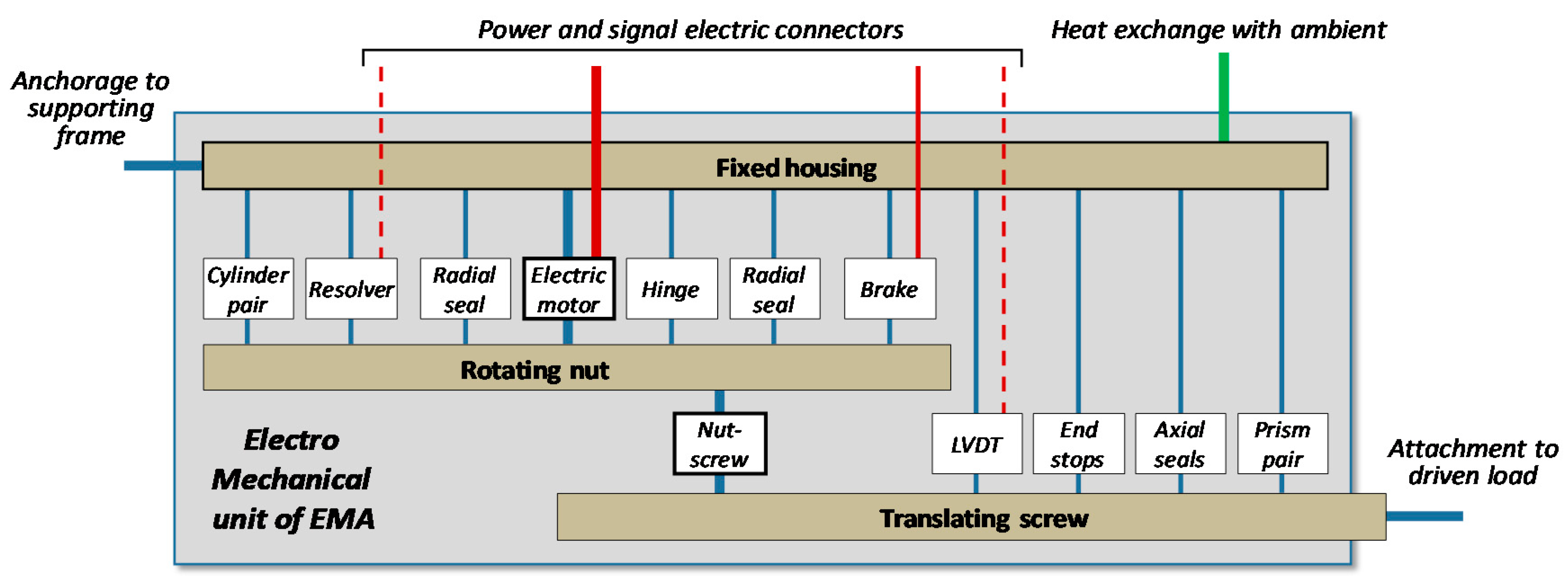
An example of electromechanical design and integration for a flight control EMA is given in Figure 1. The direct-drive electromechanical unit comprises:
- A Permanent Magnet Synchronous Motor (PMSM);
- A ball-screw;
- A rotor angular position sensor;
- A rod extension sensor;
- An electric-off brake;
- All sealing and bearing devices.
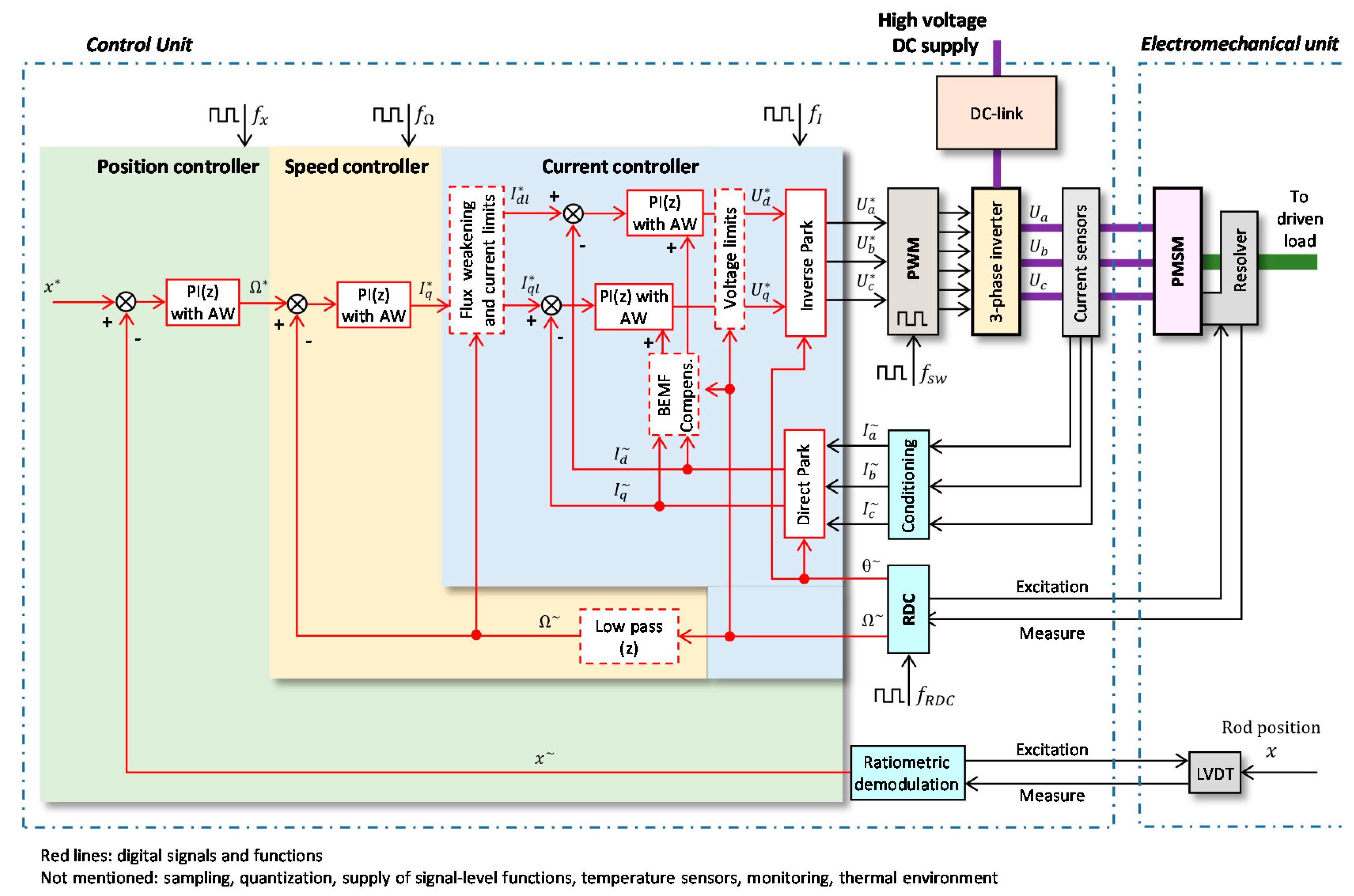
An example of the generic architecture of control and electronics is given in Figure 2 for position-controlled EMAs. It includes:
- The power electronics with the three legs of the inverter;
- The Pulse Width Modulation (PWM) switching to drive the power transistors of the inverter;
- The direct and inverse Park transforms to implement Field-Oriented Control (FOC) in the D-Q frame;
- The excitation and conditioning of current, speed, and position sensors;
- The current loops with limitations, flux weakening, Proportional plus Integral (PI) controller with anti-windup, and back electromotive force (BEMF) compensation;
- The motor speed and rod position loops with PI control and anti-windup;
- The clocks used for each control loop, speed sensor conditioning, and PWM;
- The DC-link, including the diode, capacitance, braking resistance, and chopper.
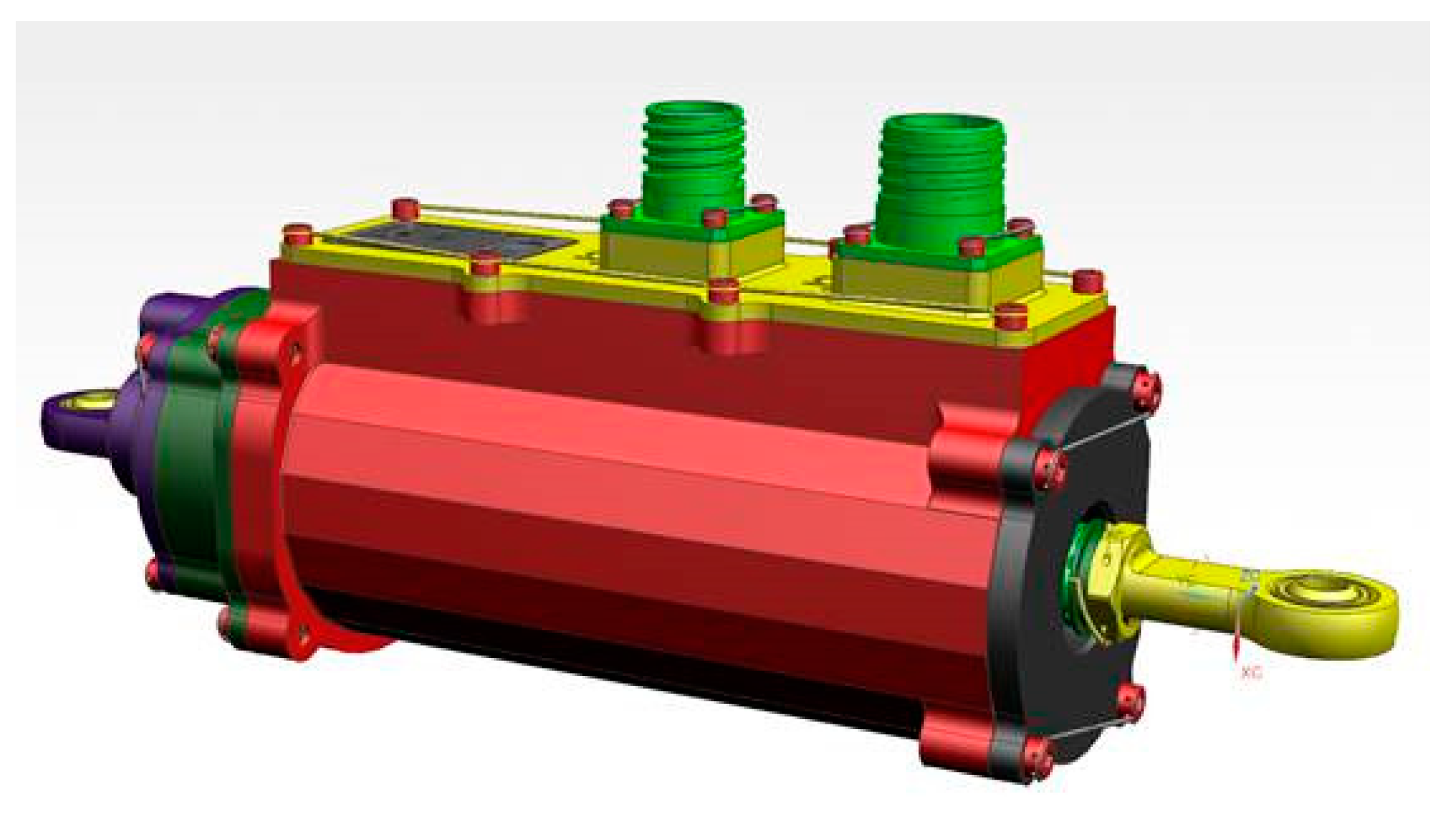
Historically, system-level simulation was introduced to support dynamic analysis and control design. With the rapid growth of MDB, progress of simulation techniques, and availability of off-the-shelf commercial simulation software, system-level simulation is now used to serve wider and wider engineering needs. For EMAs, this particularly concerns the power capability and power drawn from sources, natural and closed-loop dynamics, thermal balance, energy balance, transients during mode switching, or even responses to faults. The next sections introduce models and summarize the lessons learnt, experience feedback, and practical considerations using the illustrative example of a flight control EMA for regional aircraft; see Figure 3. The actuator has an output power of 400 W. The bandwidths of the control loops are typically 10 Hz for rod position, 100 Hz for motor shaft speed, and 800 Hz for motor currents. The sampling frequencies are set to 500, 4000, and 8000 Hz, respectively. These choices avoid significant alterations to the open-loop phase margins occurring due to the phase lags introduced by sampling.
3. Top-Level EMA Model
In an MBD process, there is a need for a top-level model of the EMA. This preliminary model is intended to validate the EMA specifications that are derived from the mission needs at the aircraft level. In particular, this involves the power capability and closed loop performances. At this stage, the main issue is to develop an EMA model that is sufficiently simple and requires a minimal number of parameters because the EMA has not yet been designed.
3.1. Proposed Model
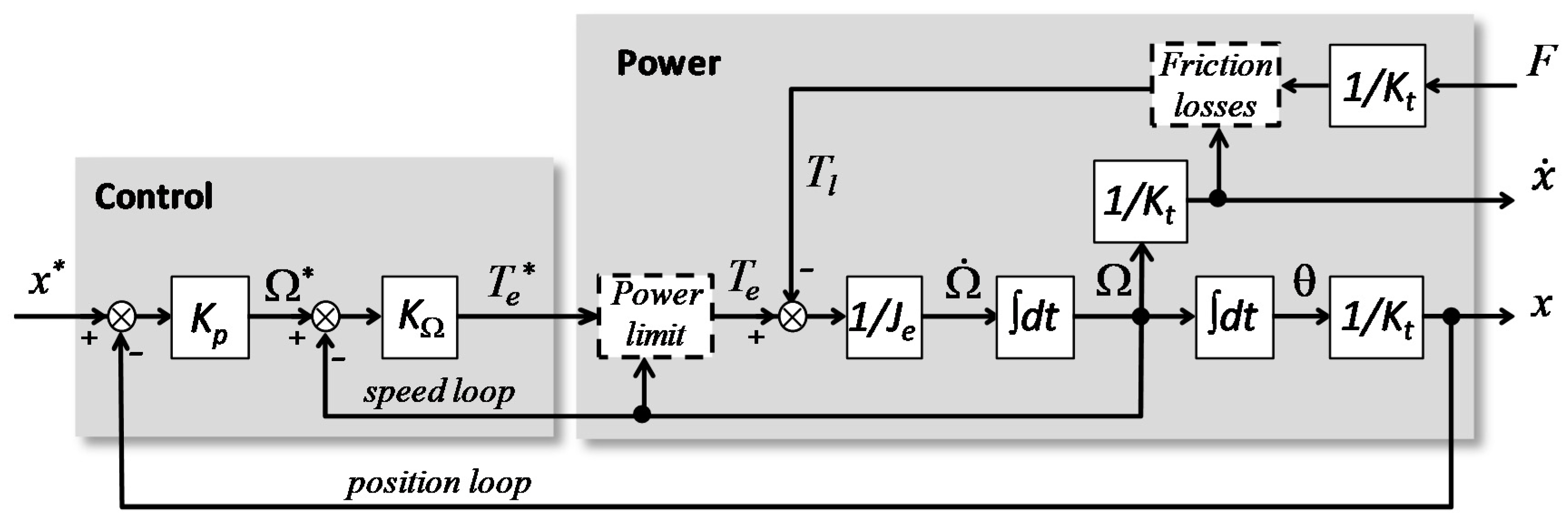
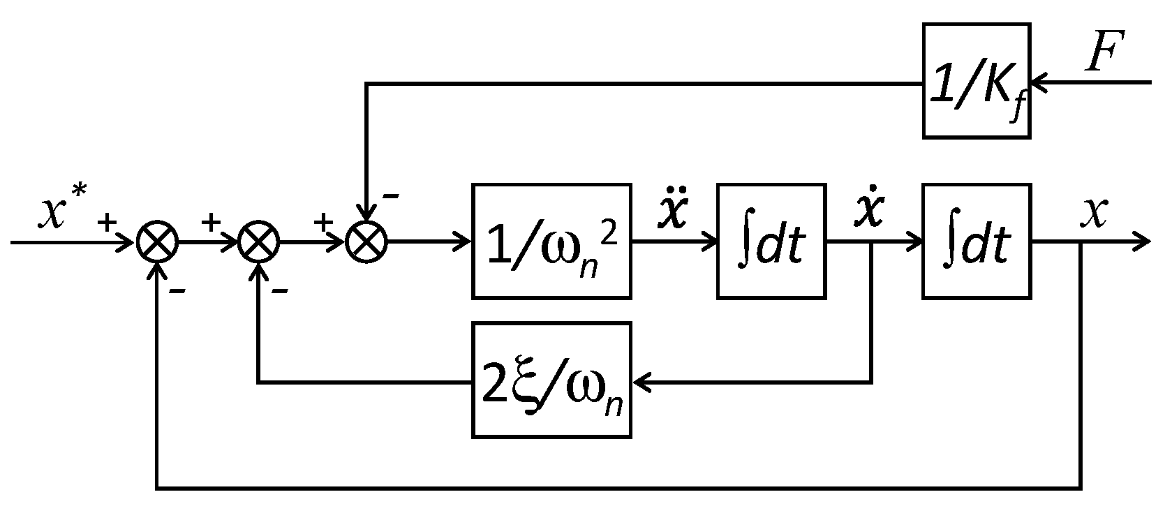
A top-level model is proposed in Figure 4. In the most common cases (flight controls and landing gears), the EMA is position-controlled: the rod extension must follow the position demand (pursuit) and reject the disturbance coming from the load force (rejection).
This model can be used in the common general case where the natural behavior of the EMA in pursuit mode is dominated by the motor rotor inertia. If other inertias, including that of the driven load, are known, they can be considered to constitute the overall equivalent inertia at the motor shaft level. The mechanical impedance of the load, which acts downstream of the position loop, can also affect the actuator closed-loop performances. Figure 4 applies in the very common case where it is of low importance: the aircraft or system designers have managed the load kinematics to avoid any flutter or shimmy, without need for force feedback for active load damping. The proposed top-level EMA model only includes an outer position control loop with a proportional control of gain . Damping is provided by an inner speed loop that controls the motor speed with pure proportional gain . The current (or electromagnetic torque) loop dynamics are considered as sufficiently rapid (around 1 kHz) to be neglected with respect to the position and speed loop dynamics (respectively, in the ranges of 1–10 Hz and 50–200 Hz in common applications). Therefore, the basic model assumes that the effective electromagnetic torque is established instantaneously and without limitation in response to the torque demand that is issued by the speed controller. In Figure 4, the block-diagram of the “Power” block, is established from Newton’s second law applied to the motor shaft. The transmission ratio characterizes the mechanical power transformation between the EMA motor shaft and rod—e.g., for a direct-drive EMA:
where is the lead per revolution of the nutscrew.
The compliance and backlash of the EMA mechanical transmission are not modelled at this preliminary level. For common aerospace applications, they are sufficiently low to have no significant effect on the power consumption. Thus, they have only little effect on the actuator closed-loop dynamics if control is properly addressed. If the power limit and frictional losses are neglected, the EMA model (Figure 4) can be simplified and redrawn as a pure second-order system, as shown in Figure 5 without dashed boxes.
In this case, the pursuit and rejection transfer functions are given by:
where is the stiffness of the closed-loop EMA.
With reference to Figure 4 and Figure 5, the position and speed proportional control gains are directly related to the undamped natural angular frequency and the dimensionless damping ratio ξ. As given by Equation (3), they only involve the transmission ratio and the equivalent rotor inertia which merges all the inertance effects of the moving bodies at the motor rotor level.
Having only two state variables and three parameters (plus a very few others related to friction and the power limit if needed), this models suits the early phases of the EMA development process particularly well, where the intention is to model the specification itself—e.g., using a Property Model Methodology (PMM) [10].
It can be seen from Equation (2) that there is a static position error under the permanent external load when pure proportional controllers are used. The addition of an integral action of gain in the speed controller removes this static dependence on the external load. This controller introduces a first-order effect of time constant:
This is an indicator of how fast the external load force disturbance is rejected. As the pole is significantly faster than the pole , there is no significant change in the pursuit transfer function , while the load rejection transfer function is multiplied by the integral effect of the transfer function .
At the project level, the top design parameters are ξ and . The control gains and are obtained from these values if the motor torque constant and equivalent inertia are known. These values can be obtained using estimation models—e.g., based on scaling laws [11]—given the range of EMA output power (velocity and force).
Beside the dominant effect of rotor inertia, power limitation and friction losses cannot be omitted if the aim is to address the EMA power capability, energy consumption, and even closed-loop stability or accuracy correctly.
3.2. Power Limitation Due to the Motor, Power Electronics, and Electric Supply
The effective motor torque is limited by several factors: electric supply, power electronics, iron and copper losses at the motor, and even the control strategy (e.g., FOC). A power limit block is therefore introduced to represent the airgap steady-state power capability, and the torque demand issued by the speed controller is thus limited by a dynamic saturation as a function of the motor angular velocity. This limitation is, for example, defined using a 1D table that covers the four power quadrants of operation. In its simplest version, the table is symmetrical and provides the stall torque at null speed, the rated torque at rated speed, and the maximal speed at null torque.
3.3. Friction Losses in the EMA Mechanical Transmission
The friction losses in the EMA mechanical transmission depend on the transmitted load and velocity (and temperature, which is generally taken to be constant for a top-level model). They are introduced into the generic model, shown in Figure 4, with a block that alters the load force as a function of velocity. As a minimum, this block has to ensure that friction forces are dissipative, opposing motion (or opposing the tendency to move in stuck conditions). A simple and common approach [12] consists of considering:
- The load-dependent friction through direct and indirect efficiencies;
- The load-independent friction through tare losses to reproduce the no-load driving torque and the no-drive back-driving load force.
Tare losses are particularly important because they directly influence the EMA power capability and thermal balance—e.g., as reported in [13].
4. Detailed Models of EMA
There is also a need for detailed models, or virtual prototypes, of EMAs to serve as virtual integration, verification, and validation. Although a single virtual prototype is welcome to address the various engineering needs listed in Section 1, the main issue comes from over-modelling. There is a wide offer of commercial simulation environments that include numerous, detailed component libraries. Therefore, it becomes extremely easy to build a very detailed multi-physics, lumped-parameter model by a click-and-drag sequence. Over-modelling thus becomes the default solution to compensate for the lack of knowledge for making decisions during the modelling process. Of course, the detailed model must be sufficiently realistic to avoid missing any effect that would change the conclusions drawn. However, over-modelling increases the computer burden for simulation and requires numerous parameters, many of which are kept at their default value in the absence of data or knowledge. The main challenge is really to actively master the modelling activity to obtain a model having just-sufficient complexity. The next sections of this paper provide key ideas and put forward some lessons learnt regarding this objective.
4.1. Dynamics in Presence
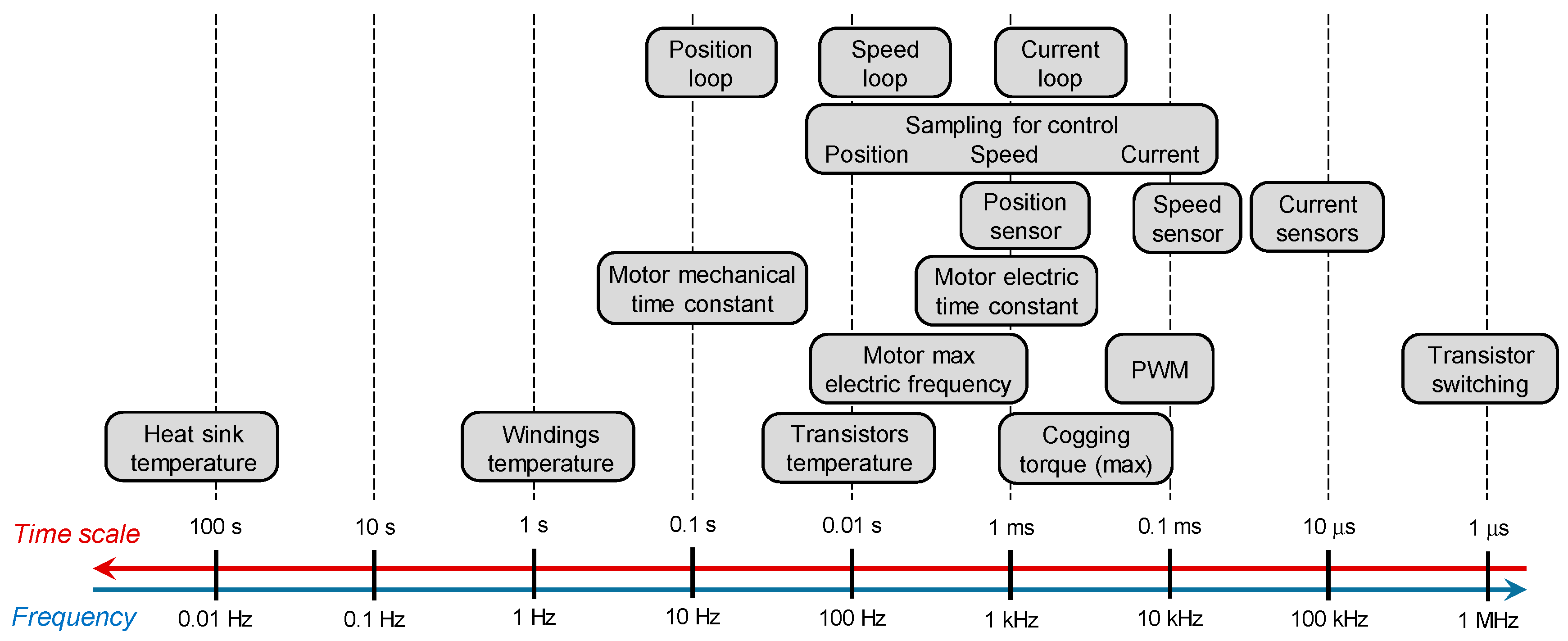
A preliminary mapping of the dynamics that are potentially present in the EMA under study provides efficient support to the model development. As it comes at the beginning of the detailed modelling process, this mapping does not require accurate values. However, it can be updated as the project goes on, at least for capitalization, to provide inputs to future projects. It is important to note that this mapping is a source of important information for decision-making during the development of real-time models for integration tests [14]. An example of such mapping is given in Figure 6. The limit of time scales reproduced by the model is set according to the modelling objective.
4.2. Modelling Needs vs. Engineering Needs
Another way to support decision-making during model development has been applied with success [15]. In particular, it facilitates discussions between project leader, partners, domain experts, and person(s) in charge of simulation. It consists of making a table that links the engineering needs (columns) to the phenomena that must be modelled or can be ignored (lines). An example is given in Table 1, which is inspired by [15]. Different levels of models (e.g., functional, basic, advanced, expert) are identified and configured for each engineering need. In that manner, the model development follows an incremental process, in phase with the project progress. Each cell must be marked as mandatory (M), optional (O), or useless (U). In addition, it is worth introducing the consequences of modelling choices on the model complexity and computation burden, as shown on the right side of the figure. The following sections focus on the phenomena that generally give rise to much discussion and many modelling issues.
5. Detailed Modelling of the Power Chain
5.1. Motor and Power Electronics
The modelling of power electronics and motor cannot be done independently, as the model interfaces must match. In practice, there are only a few possible combinations that are really interesting in an MBD approach. Although rarely addressed, modelling the DC-link is important, as it impacts the voltage supply of the inverter, the heat losses, and the spikes generated in the electric supply.
5.1.1. Motor Model
As mentioned in Table 1, there are different modelling levels for the EMA motor. In a progressive modelling approach, it is therefore of major importance to ensure continuity between the uses of these models, in particular by keeping the same current controller setting and supply parameters. However, common models do not meet this continuity constraint and the simplest equivalent DC models—e.g., [16]—do not address control, heat losses, and electric power consumption simultaneously.
This section intends to meet this need. The motor model development has followed a bottom-up approach (from the three-phase to the top-level model) in order to easily identify how to enhance the common DC model in order to reproduce the effects coming from the three-phase realization of the motor.
Three-Phase Model and Motor Constants
A three-phase model (e.g., [17]) has the same physical electrical interfaces as the motor under study, as shown in Figure 2. Consequently, it directly connects to the model of the three-leg inverter. Realism can be progressively increased—e.g., as in [18]—to make an expert-level model that includes cyclic inductances, cogging, magnetic saturation and iron losses, and multi thermal bodies. In practice, significant work time and effort are wasted, in particular in collaborative projects, due to a misunderstanding of the motor parameters and variables that are used by their models. The PMSM constants, whatever the type of model considered, are hardly ever given with sufficient information: peak or Root Mean Square (RMS), line-to-line (LL), or line-to-neutral (LN). Figure 7 is introduced to settle this issue and avoid any misunderstanding. In particular, it clearly points out when the BEMF constant and torque constant are equal and have to be used in the equivalent DC model of the PMSM to be power conservative. The relations between the different BEMF constants follow the relations between voltages, while the relations between torque constants are the inverse of the relations between currents. It is also important to mention explicitly how the resistance and inductance of the windings are defined (line-to-line or line-to-neutral).
Two-PhaseMmodel
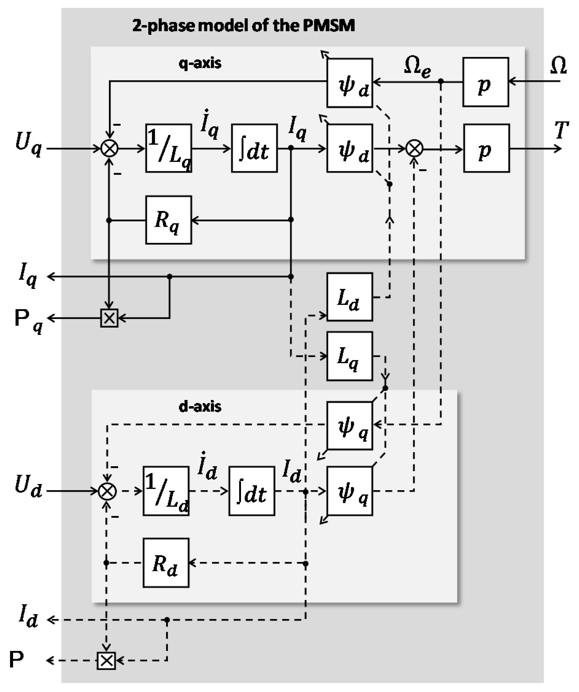
The Clark and Park transforms enable the three-phase model to be expressed as a two-phase model using the d-q (direct-quadrature) frame [17]. Such a model is mainly used as a control to simplify the control design and implementation, as mentioned in Figure 2. It is often implemented internally in three-phase motor models because it reduces the model order (two instead of three) and involves variables that are useful for motor operation analysis. The direct dq0 Clark/Park transform establishes a link between the electrical quantities (voltages or currents) when they are expressed in two different frames. Frame a-b-c corresponds to the electrical ports of the motor for a star winding connection. Frame d-q corresponds to the direct and quadrature axes attached to the rotor. The dq0 transform given in Equation (5) combines the Park transform [19] and Clarke transform [20]. When power and energy considerations are of interest, it is preferred because it is power-invariant, unlike the Park transform, which is voltage-invariant (factor is not present).
The elements of the transformation matrix are time-dependent as they use the motor electric angle (the rotor/stator relative angular position , where is the number of pole pairs of the motor). Figure 8 displays a block-diagram model of a non-salient pole motor in the d-q frame, when the dq0 transform is used. Dashed lines emphasize the influence of the d-axis on the q-axis.
The magnetic fluxes in the d-q frame are expressed as:
From a pure control view, the d-q model is interesting because it can be directly connected to the and current controllers. However, pure two-phase motor models are rarely used when energy (conduction and switching losses at inverter), power limitations (supply voltage), and switching strategy (space vector modulation) have to be considered. In this case, they need to interface with an equivalent two-phase inverter model, which is not easy to develop.
Equivalent DC Motor Model
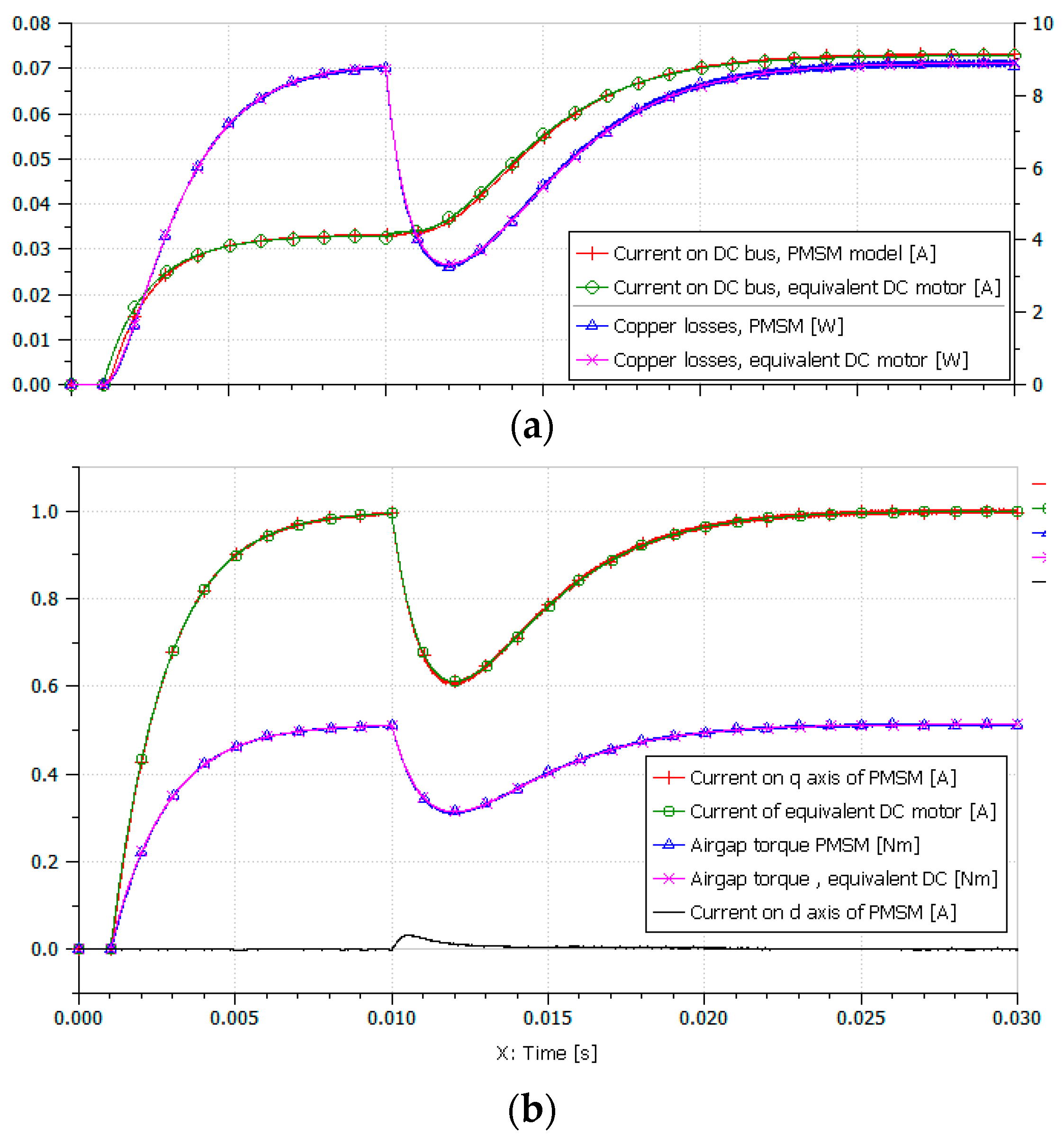
Equivalent DC motor models are used extensively for their simplicity (a single-state variable, no trigonometric functions), in particular during the early phases of design. Unfortunately, the models published so far—e.g., [16]—are not intended to reproduce the dynamics, power drawn at supply, and heat power simultaneously. The equivalent DC model proposed in Figure 9 is easily derived from the d-q model if the current is assumed to be null at all times.
All the dashed lines and associated blocks have therefore been removed in Figure 8. This condition is achieved with a perfect FOC, implementing a constant torque angle control [17]. According to Figure 7, the and constants are equal. The winding resistance and inductance are taken line to neutral. In the linear domain of the PWM operation, the available line-to-line RMS voltage is . Figure 10 compares the responses of the full model of PMSM (Figure 2) and the equivalent DC model (Figure 9).
The results are obtained in the following conditions:
- Only a current loop is implemented with a P-I controller. The controller gains and sampling frequencies are identical for both models.
- The system is at rest at time 0 (no current demand, no rotor speed). A step current demand is applied at time , then a step motor speed is imposed at time . With these excitations, the operation remains below the saturation limits.
- Both models are supplied with the same constant DC bus voltage.
- Current sensors are perfect in both models.
- In the full model, a symmetric triangle PWM is used to drive the three-phase inverter. The * setpoint is set to null. Flux weakening and BEMF compensation are not enabled. The losses in power electronics are quasi null. The current controller makes the current loop five times faster than the one.
It is clear that both models produce the same responses for the three engineering needs addressed:
- Control design: same static and dynamics for current and torque.
- Thermal balance and energy losses: same motor copper losses.
- Power drawn: same current from DC voltage source, thanks to the factor in the equivalent DC motor model.
It is, however, important to recall that this excellent equivalence is altered when saturation occurs. This is the price to pay to obtain a simplified model. Firstly, the voltage induced by the current and the rotor speed (coupling effect visible in Figure 8) represents a non-negligible part of the maximum voltage . Secondly, the current can be demanded by the controller in the case of flux weakening, or generated by the motor when its control is lost due to the saturation of the duty cycle demand. In practice, there is a beneficial effect as the PWM can operate in a pseudo linear range when the duty cycle demand does not saturate too much [21]. Extending the operation over this range and even over the non-linear range generates unexpected current with all its above-mentioned effects. In these conditions, it is almost impossible to make a single equivalent DC motor model that is simultaneously representative of the power capability, power consumption, and energy losses.
5.1.2. Model of Power Electronics
Whatever the type of electronic control of motor power (H-bridge for DC motors, inverter for PMSM), several modelling options exist. For each leg, the association of two independent models, one for each solid-state switch, generates an algebraic loop for the calculation of the leg output voltage. This issue is resolved by making a single model of the whole leg in which the two cell models are combined analytically.
Linear models can be simulated quickly. They merge the diode and transistor conduction characteristics to make a single linear resistor for each commutation cell. As far as non-linear models are concerned, the voltage threshold and switching losses (possibly plus other effects) are considered to reproduce the energy losses with better realism.
Averaging can also speed up the simulation significantly, as no switching events occur. Full averaging applies to the whole leg set. It delivers the motor line voltages (, , ) vs. the voltage demands (, , in Figure 2) without any need to model the PWM. Intermediate averaging calculates the mean operation during one PWM period for each leg. Of course, averaging reduces the realism of the simulation, in particular regarding the ripple and energy losses in the presence of significant electric load inductance.
When the model must reproduce the control performance, the power capability, and the energy consumption at the same time, it is mandatory to resort to non-linear, non-averaged models of the power electronics.
5.1.3. Model of DC-Link
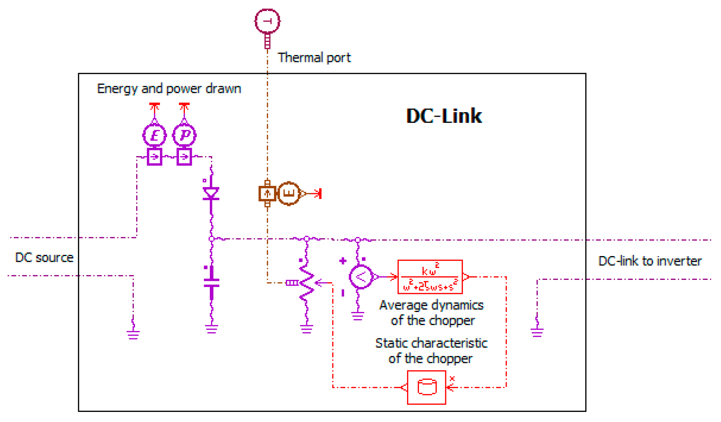
The DC-link supplies the power electronics that control the motor. Its operation performs two main functions: it stores electric energy to meet the high transient current demands from opposite loads, and it avoids regenerative currents being sent back to the centralized power source under high aiding loads. However, its operation also generates side effects. The DC-link voltage is not constant; regenerative power is transformed into heat power when the DC-link voltage reaches the acceptable limit. It draws transient positive currents to charge the capacitors when the DC-link voltage drops below the allowed value. In an MBD approach, it is therefore important to make a DC-link model reproducing both functional and parasitic effects. This helps to assess the closed loop performances, thermal balance and stability, and energy consumption. It is also a precious means of validating the sizing of the power components of the chopper. Modelling the DC-link is generally not considered for EMA simulation—e.g., [22]. A DC-link model is proposed in Figure 11. In this simple version, the chopper average operation is modelled using a variable resistor that is piloted according to the DC-link voltage. The table reproduces the static characteristic, while the second-order model reproduces the mean dynamics. From a numerical point of view, it also serves to avoid an algebraic loop. Once again, the model is thermally balanced thanks to the thermal port. Energy and power sensors are added for analysis.
5.2. Friction
Friction M&S must be addressed with care, because it directly affects the soundness of the conclusions drawn from simulated responses. This concerns the closed-loop performance (accuracy and stability) in particular, as well as the power capability, thermal balance, and energy consumption. Friction losses appear at many locations in EMAs: mechanical motion transformation (e.g., nutscrew or gears), bearings (e.g., axial thrust bearing or anti-rotation), joints (e.g., eye ends or gimbals for anchorage to supporting a frame or attachment to a driven load), plain bearings (e.g., for cylindrical pairs), or power management devices (e.g., brake, clutch, or torque limiter). Moreover, friction is caused by various phenomena at each location: rolling, sliding, drag, churning, splashing, etc. This makes friction M&S at the EMA level really challenging.
5.2.1. Time-Dependent Variables Affecting Friction
In the field of control, friction is generally viewed as a speed-dependent phenomenon. Starting with pure viscous friction, models enable linear analysis to be employed widely for preliminary control design. Commonly, the models are then improved for numerical simulation, considering Coulomb friction, Stribeck, and Dahl effects. Load and temperature effects are ignored most of the time. In contrast, in the field of mechanical design, friction is considered as mainly load-dependent, in particular with the extensive use of mechanical efficiency for power sizing. Temperature and speed effects are only partly documented in component datasheets [23].
According to tribology fundamentals [24], sliding friction forces can be expressed as the product of the normal force at contact and the friction coefficient. This coefficient depends on the Hersey number, SN, which involves the kinematic viscosity, , of the lubricant medium; the relative speed of facing bodies at contact, and the pressure, in the lubricant medium at the interface between bodies. Unfortunately, the lubricant viscosity depends hugely on temperature—e.g., in a 370:1 ratio between −40 and +100 °C [25]. Therefore, it is clear that, for a given design, the sliding friction depends on the temperature, relative speed, and normal load at contact. It is interesting to generalize this dependency to make a generic friction model that also applies to other sources of friction—e.g., as documented by ball- or roller-bearing suppliers [26].
5.2.2. Management of Sticking/Sliding Transition
The numerical management of the transition between sticking and sliding states is a well-known issue in friction M&S. This comes from a change in causality for friction calculations; in sticking conditions, the friction force opposes the other forces, while in sliding conditions, the friction force opposes relative motion. There are many candidate solutions for this issue which have been extensively documented—e.g., [27,28,29]. The most common ones are available in the commercial simulation environments:
- The hyperbolic tangent model is very simple to implement, involving a single parameter to manage the sticking/sliding transition. It enables each location of friction be modelled independently. The main drawback lies in its inability to produce true stiction, unlike the following models, because the simulated friction force is null at null speed. Moreover, it may generate numerical instability in particular cases. This is due to the huge equivalent viscous effect produced near the null relative speed to smooth the sign function.
- The Dahl and Reset Integrator models, or their generalization as the LuGre model, solve the transition issue by considering the compliance of the asperities of the facing surfaces in sticking conditions. This additional energy storage effect solves the causality issue by introducing a first-order differential model. Unfortunately, the combination of contact stiffness with inertia effect generates high-frequency natural dynamics that significantly increases the computational burden of the integration algorithm. In practice, there is generally no engineering need to model this compliance, except in very specific cases such as mirror positioning for imaging satellites. Nevertheless, this type of model is often used implicitly for its ability to solve the transition issue.
- The “rendez-vous” model is very efficient but requires the numerical solver to be able to accurately locate a state-event between two integration steps (external forces exceeding the breakaway friction force for starting, or speed crossing zero for possible stopping). It also generates a multitude of search functions that significantly increase the computational burden.
- Non-causal simulation languages—e.g., Modelica [30]—and associated solvers enable a particular type of friction modelling that also reproduces true sticking. As an additional advantage, they also allow inverse simulation, which is welcome for sizing. However, non-causal friction models are implemented with assumptions for inverse simulation that are not always explicit. So far, it is the author’s experience that industry sometimes hesitates to switch to these tools because the engineers concerned are not sufficiently experienced and they fear that the tools may be insufficiently mature for use in industrial projects.
- The Karnopp model is efficient to reproduce the true stiction and manage the sticking/sliding transition with a little computational expense. It uses a single parameter, the velocity threshold, below which relative speed is forced to null. Unfortunately, this means that the model is intimately linked to the inertance model (mass for translation, moment of inertia for rotation). Therefore, the friction model cannot be dissociated from the inertance model—with all the consequences for causalities (e.g., difficulty in simulating friction between two moving bodies, or multiple frictions on a single body).
5.2.3. Proposed Generic Friction Model
According to the previous section, it is considered that a generic friction model meeting the engineering needs for EMA design must:
- Aeproduce true stiction at the lowest computational expense;
- Enable multiple locations of friction to be modelled for a single rigid assembly;
- Enable the load, temperature, and velocity effects to be considered;
- Enable implementation within a wide set of commercial simulation environments, in particular without resort to non-causal simulation languages and associated SW;
- As far as possible, reuse a friction model from the standard library of the simulation SW, which is documented, verified, and numerically robust.
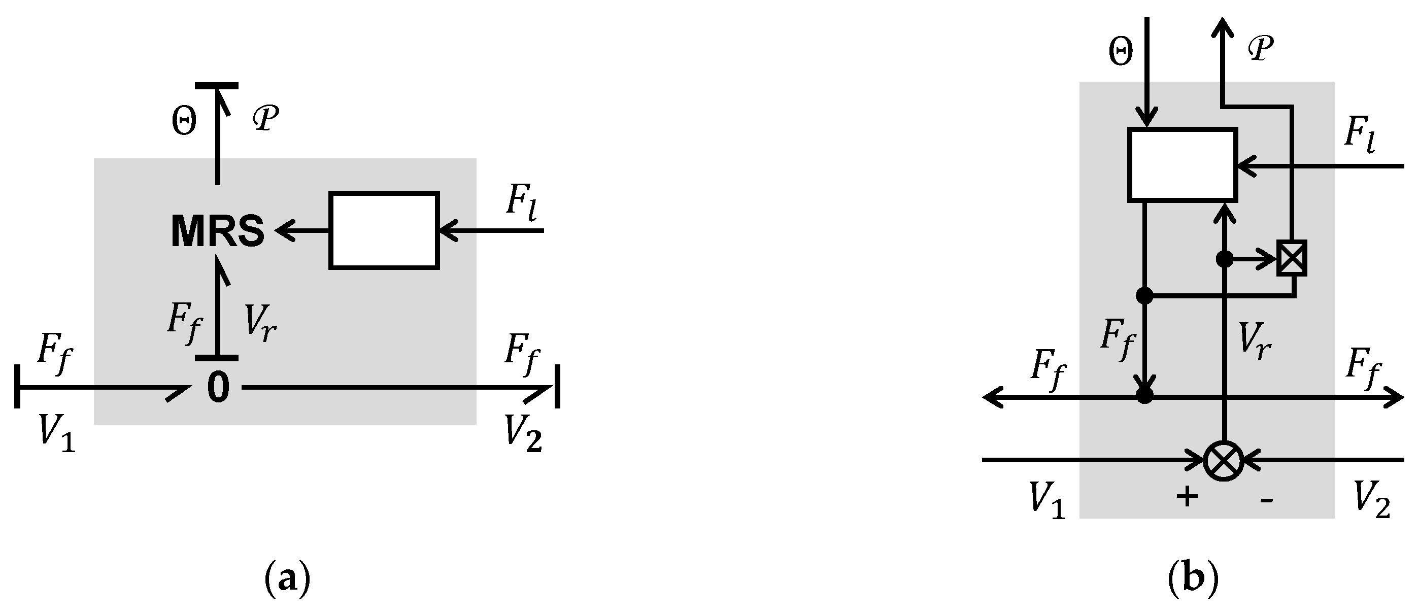
- Independently of the management of the sticking/sliding transition, the proposed friction model architecture is given in Bond-graph and block diagram forms in Figure 12. It involves:
- Two mechanical power ports that feed the model with the linear velocities, and , of each of the facing bodies (or angular velocities and ), and obtains the friction force (or torque ) applied to each facing body from the model.
- A thermal power port that feeds the model with the temperature at the contact interface, and gets the heat power generated by friction from the model.
- A signal port that inputs the transmitted load force, (or torque ), to introduce the effect of the normal force at the contact location.
- A parametric function or a multi-D table that shows the friction force vs. relative speed, temperature, and transmitted load.
Thus, the generic friction model is ready for use whatever the contributing factor considered. The load force affects the friction force not only through its magnitude but also through its sign, which, when multiplied with the relative speed, determines the power quadrant of operation (aiding or opposite load). The sign of the external load itself may directly affect friction in very particular cases—e.g., in non-symmetrical axial thrust bearings for landing gear-extension/retraction EMAs. In any case, the proposed model architecture ensures energy balance at the model interfaces. It can be transposed for the friction torque by replacing forces with torques and linear velocities with angular velocities. This generic model has been successfully implemented in various simulation environments, such as Matlab-Simulink, AMESim, and Dymola-Modelica.
5.2.4. Application to EMA
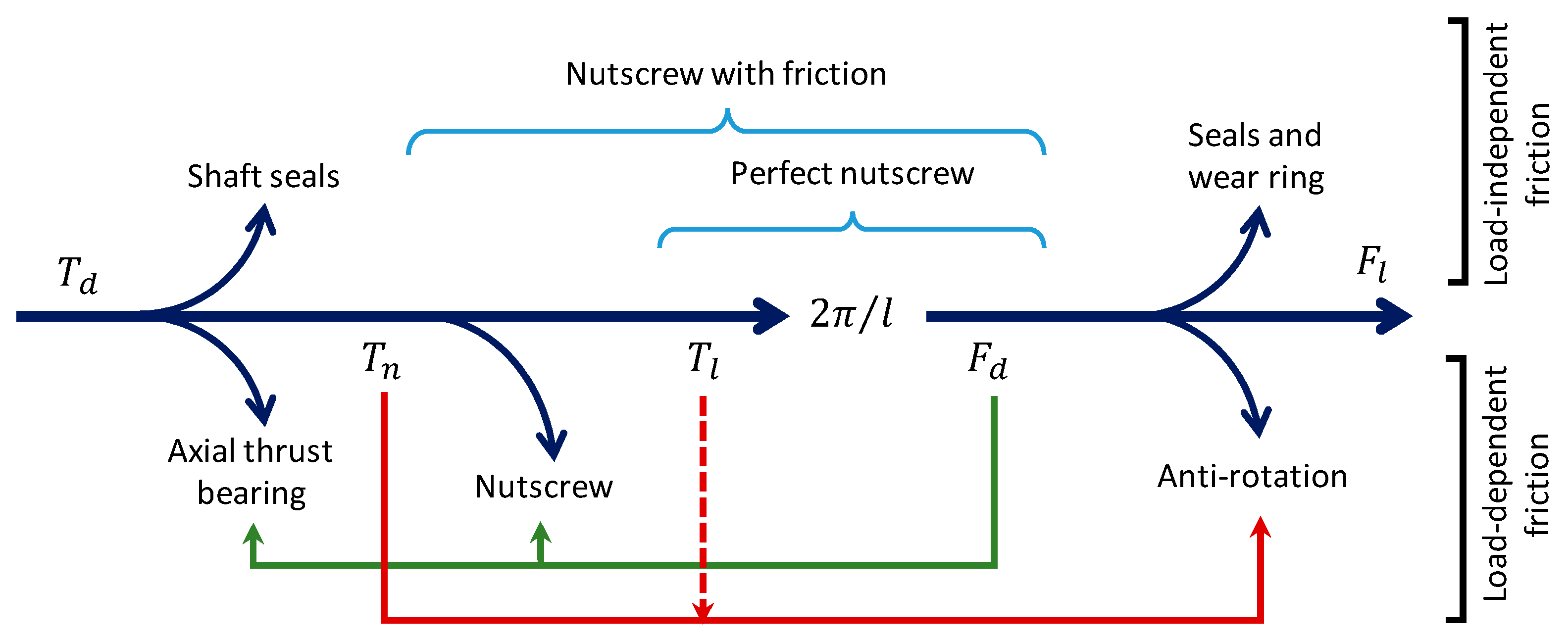
Two moving assemblies, each forming a rigid body, can be identified in Figure 1. The rotating one includes the motor, the resolver and brake rotors, the inner races of bearings, and the screw nut. The translating one includes the screw, EMA rod, Linear Variometer Differential Transformer (LVDT) measuring the rod extension, and ball joint lug end. The anti-rotation device is intended to make a prism pair between the screw and the EMA housing. It balances the screw torque that is transmitted by the nut. Therefore, it generates a friction force on the rod that depends on the torque driving the screw. The transverse loads at rod seals and wear ring are negligible, making their friction force quasi load-independent. Similarly, the axial thrust bearing is intended to balance the axial force produced by the screw on the nut. It generates a friction torque that depends on the axial force developed by the screw. The friction of seals on the rotating assembly is load-independent. The nutscrew friction applies between the nut and the screw, but its detailed modelling is not straightforward [31] and requires parameters that are difficult to handle. For this reason, the common approach is to lump the nutscrew friction at either its rotating or its translating side. In the proposed model, it is considered at the rotating side, as illustrated in Figure 13.
It is worth noting that the present model does not consider transverse loads that are generated on the EMA bodies. However, such forces are introduced in practice by friction (at EMA anchorage to supporting frame and transmission to load) and inertance effects (e.g., pivoting of the EMA in a three-bar mechanism). If necessary, a 2D or 3D lumped-parameter model of the EMAs and their kinematics to load can be developed using the mechanical libraries of the simulation software. In this case, the external load used to modulate the friction model becomes a compound value—e.g., made up of radial and axial forces for ball bearings. However, such a 2D or 3D mechanical model requires numerous additional parameters, such as the stiffness and damping matrixes at each hinge joint. These parameters are generally unknown. The addition of high stiffness generates high-frequency dynamics that significantly slow down the simulation. This is why these effects are generally not modelled, as long as the transverse forces remain much lower than the axial forces.
The presence of various locations of friction sources acting on a single moving assembly can be dealt with in different manners for simulation. As the intention is to reproduce true sticking, tanh friction models must be set aside. Lugre models would require local deformation of contact asperities to be introduced at each friction location. This would require highly uncertain parameters to be set and add unnecessary dynamics that would hugely increase the computational load. Non-causal simulation tools cannot yet be considered as available for any team in charge of simulation, in particular in a collaborative environment. Moreover, they have not yet demonstrated their robustness for the simulation of multiple sources of friction applied to a single moving assembly. For all these reasons, preference has been given to the Karnopp friction implementation (but keeping its drawbacks in mind).
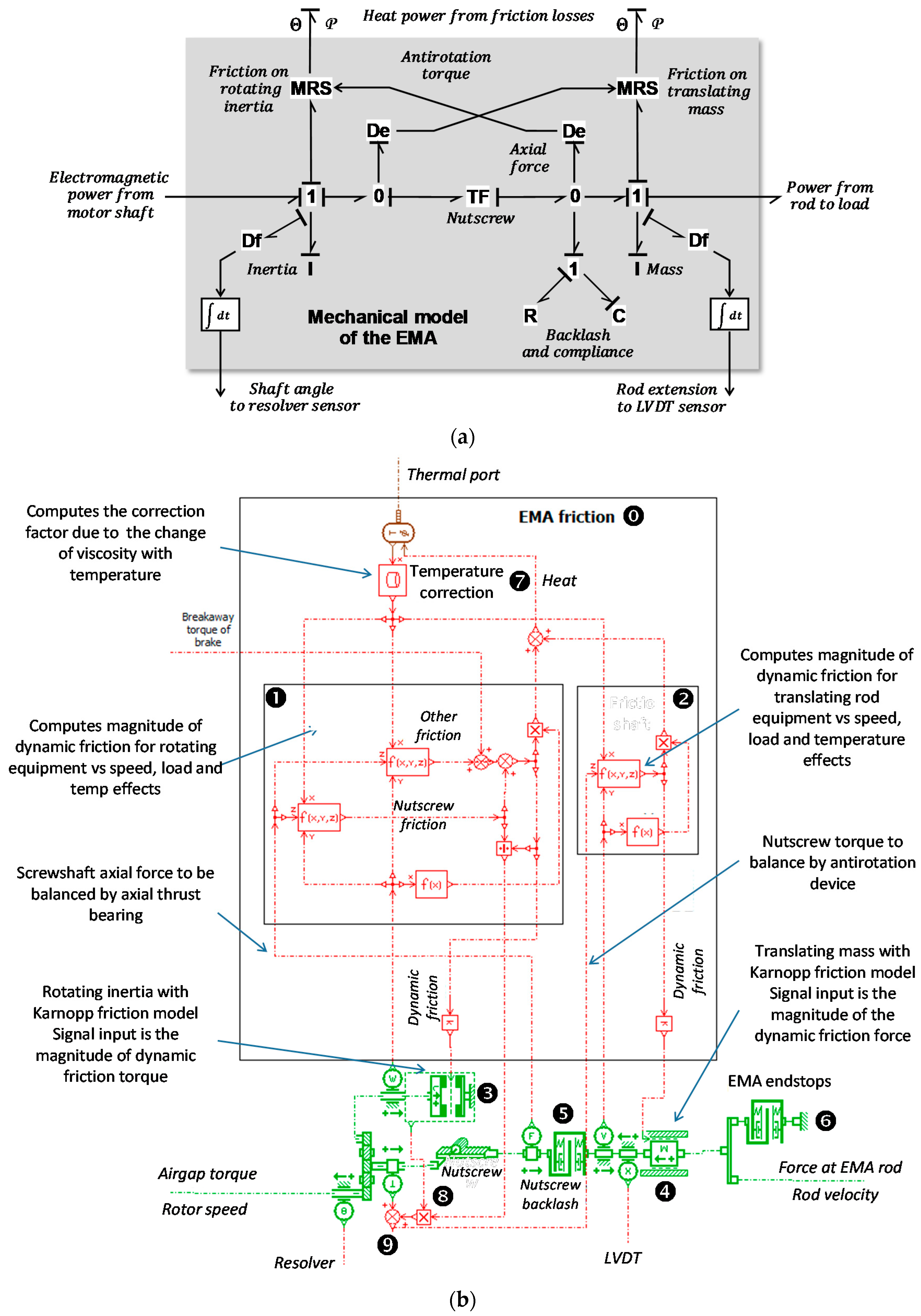
An example of model structure and implementation is given in Figure 14. For simplicity, it is assumed that there is no motion of the EMA housing. The Bond-graph models friction with two modulated RS fields. According to the causality bars, the bond to the 1 junction introduces the speed effect (R part of the MRS field), while the temperature effect comes from the thermal bound (S part of the MRS field). The load effect comes from the modulation signal (M part of the MRS field) that senses the force or torque concerned through effort detectors (De).
The model of the EMA mechanical parts links the motor shaft power port (airgap torque and angular velocity) to the EMA rod power port (force to load and linear velocity of extension) functionally through a perfect rotational/translational transformation (nutscrew). The model outputs the shaft angle and rod position to feed the resolver and the LVDT sensor and conditioner models.
The friction model ⓿ combines the friction torque on the shaft ❶ and the translational friction on the rod ❷. The inertia effects (inertia ❸ of rotating bodies and mass ❹ of translating bodies) are included. On the translational side of the nutscrew, a single model ❺ merges the overall backlash and axial compliance of the EMA (nutscrew plus axial thrust bearing). Rods to the housing end stops are included as an elastogap ❻. All the contributors to friction on a given rigid assembly are merged to calculate the magnitude of the dynamic friction and torque. These values are sent to the inertia models that include the Karnopp implementation for sticking/sliding transition. In that manner, the friction forces/torque in sticking conditions are calculated by the inertia models. The friction model also receives the magnitude of the breakaway friction torque of the brake that is added to the contribution of other friction locations. All the friction models feed the heat port with the heat generated by friction, while the friction calculation is made sensitive to temperature through the correction factor in ❼. There is no causality issue, as the inertia/friction models are connected through the backlash/compliance model.
The use of Karnopp friction models introduces a specific issue here: the calculation of the friction force generated by the anti-rotation device on the EMA rod uses the torque applied to the nut, including friction. However, the shaft inertia model handles only the overall friction torque, including that of seals and axial thrust bearing. The solution proposed consists of calculating the magnitude of the nutscrew dynamic friction torque separately in ❽. This enables its relative contribution to overall friction torque to be determined. It is then assumed that this relative contribution remains constant at all times. Therefore, this ratio is applied to the actual friction torque computed by the Karnopp approach of the shaft inertia model in ❸. This gives the actual nutscrew friction torque that can be summed in ❾ with the frictionless nut torque in order to feed the rod friction calculation module ❷. Of course, the friction model presented in Figure 14 can be implemented in a script version instead of using a block-diagram representation. There is also no specific problem with applying the proposed approach to gear-drive EMAs. In this case, each additional moving assembly has to be combined with a transmission compliance/backlash to avoid any causality issues.
5.3. Compliance and Backlash
There are various ways to model compliance and backlash, as reviewed in [32]. Whatever the solution used, the model requires a few parameters that are difficult to set without a trial and error process: damping at contact and (if used) limit penetration for full damping for the elasto-backlash model in addition to the reference speeds for the Karnopp friction models. This is emphasized when the deformation is modelled as a power function of load, in order to reproduce the non-linear stiffness of Hertzian contacts. However, these parameters can be pre-set using simple considerations:
- The viscous damping coefficient at contact can be determined to produce, e.g., a 0.2 dimensionless damping factor when it combines the contact stiffness and attached load inertia to make a second-order dynamic.
- The limit penetration for full damping can be set, e.g., to 1/100th of the backlash, or 1/10th of the elastic deformation of the contact under the rated load.
- The reference speed for the Karnopp friction model can be set, e.g., to 1/10,000th of the rated speed or, e.g., 50% of the resolution of the speed measurement.
As it is generally impossible to identify these parameters from measurements, the pre-set parameters have to be adjusted using a trial-and-error process to produce a realistic simulation (a few rebounds) without excessive computational burden. Using this approach, the model of the EMA mechanical transmission, including friction and elasto-backlash, has shown an excellent robustness with a short execution time. Such models have also been implemented in the Matlab/Simulink environment without difficulty. It has to be noted that setting the contact parameters is more tricky when the deformation is modelled as a power function of the load, in order to reproduce the non-linear stiffness of Hertzian contacts.
6. Detailed Modelling of the Signal and Control Chain
As pointed out for the power chain, several improvements in modelling practices for the signal and control chain can make the MBD of EMA more efficient. Proposals generated by experience feedback apply at all levels: controller and digital implementation (including parameters and timing), sensors and conditioners (including position, speed, and current measurements).
6.1. Control and Digital Implementation
6.1.1. Controller Parameters
The EMA control may include flux weakening, the limitation of setpoints, and BEMF compensation. These functions involve:
- The motor rotor angle and speed and the phase current signals.
- The motor parameters, such as the BEMF constant, winding resistance and inductance, and number of pole pairs.
Respecting the difference between the parameters used by the motor model and those used in the controller setting is of prime importance as the motor effective parameters vary with time, at least in response to temperature changes. It must be kept in mind that, for a 100 °C temperature increase (much lower than in real life at the actuator level), the electric resistivity of the copper increases by ~40%, the voltage offset of the IGBT transistors increases by ~25%, and the magnetic induction of the samarium-cobalt magnets decreases by ~4%. This justifies the need to make the EMA component models sensitive to temperature in order to validate the robustness of the controllers.
Another important point during modelling is related to the output limits for each controller. These have to be set with care, but this is hardly ever mentioned. It has been verified that a proper setting, as proposed in Table 2, avoids excessive saturation at the PWM function. This helps to keep the motor under control by avoiding unexpected current.
6.1.2. Timing for Digital Implementation
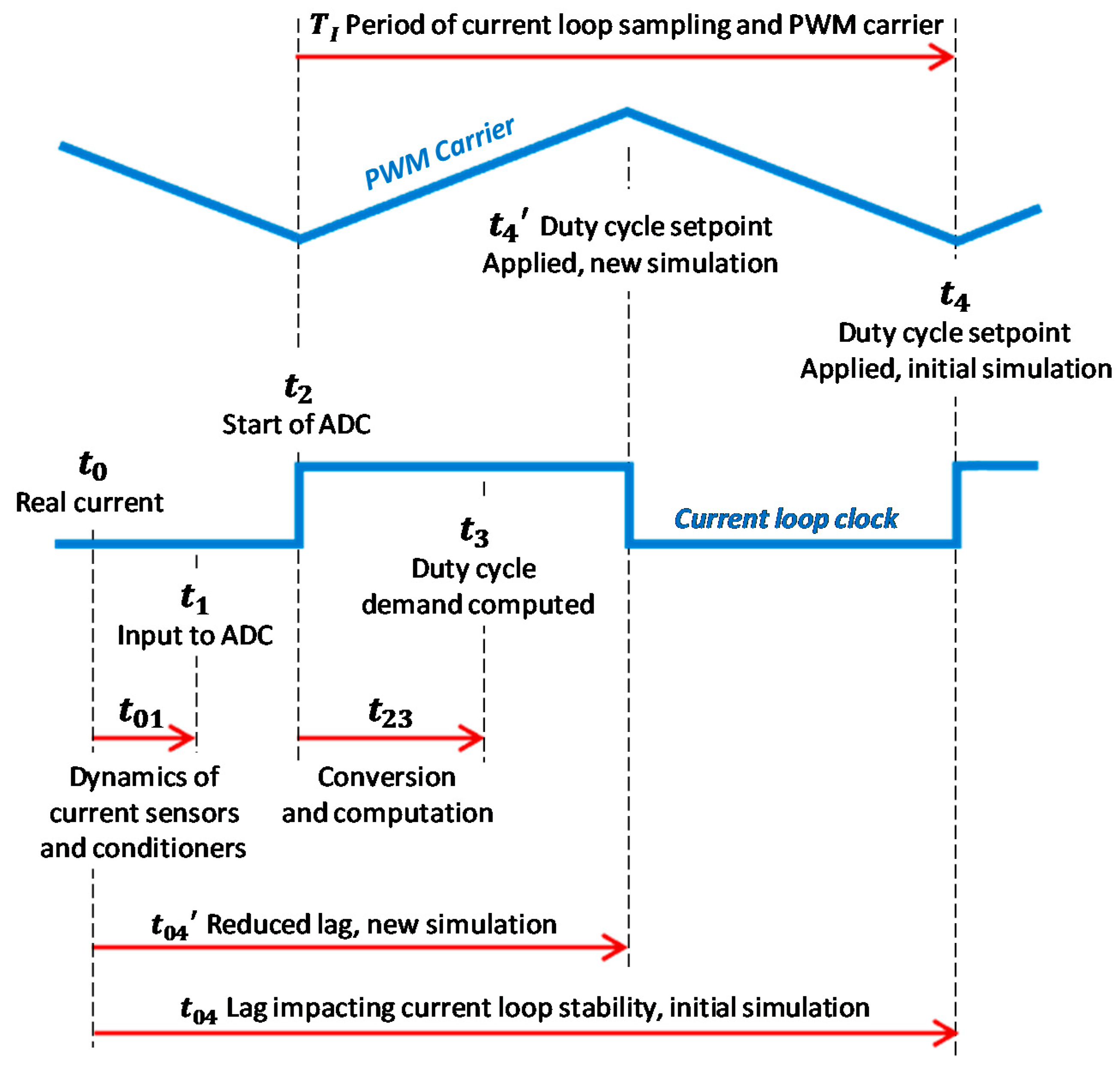
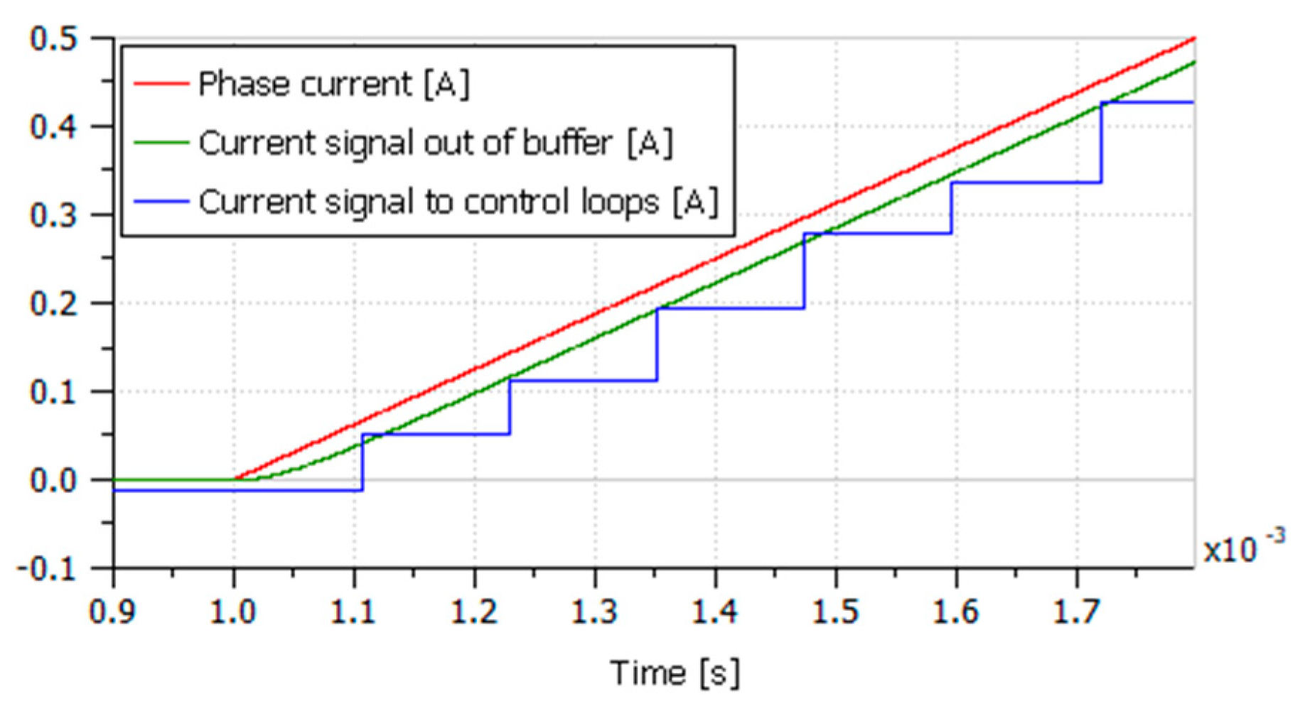
The timing of the control loops and PWM can significantly affect the EMA closed-loop performances, in particular for the current loop, which is the most dynamic one. Beside sensors and signal conditioners, the computation of the control laws, sampling, conversion (analog to/from digital), and updating of the PWM all generate time lags that increase the open-loop phase lag, with its negative effect on the closed-loop stability. These effects are usually modelled by merging them into a single first-order lag model—e.g., [21]. In an MBD approach, a proper simulation of this timing as early as possible has been found to be very fruitful. It enables the choices made for implementing the controllers to be assessed, in particular regarding consistency between the expected closed-loop performances, control design output, and selected software/hardware solutions. This particularly applies to the relative timing between the current loop sampling and PWM update, as illustrated by the following example.
In this application, the current loop sampling period and PWM carrier period are identical (noted ). The PWM is implemented using a symmetrical triangle carrier. In the first simulation, it was implicitly assumed that the PWM was updated in phase with the current loop clock, as in Figure 15, introducing a total time lag of between the real current and the update of the PWM.
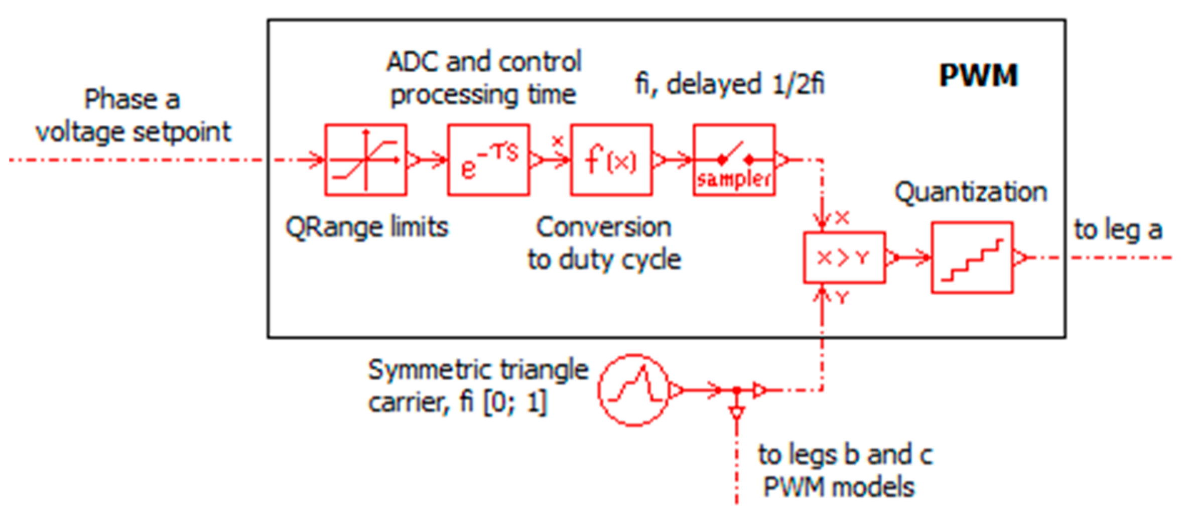
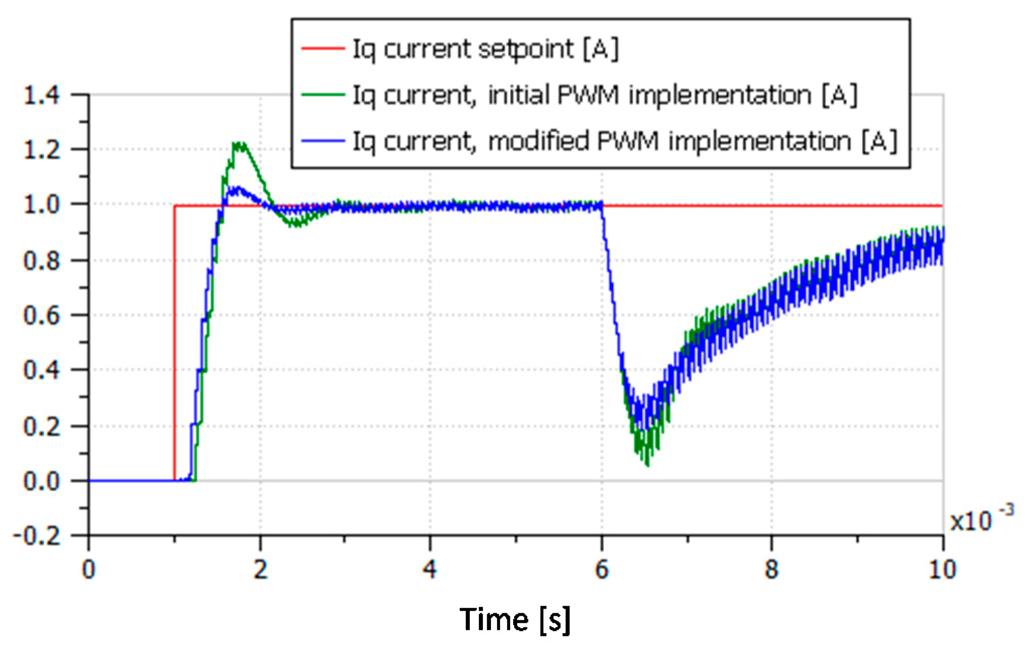
The preliminary estimation of the time spent for the Analog-to-Digital Conversion (ADC) and computation of the control law gave a value lower than . This small value suggested that the PWM update should be specified at the falling edge of the current loop clock. With a new value of , the total time lag was reduced by 36%. An example of model implementation is given in Figure 16. The improvement is illustrated in Figure 17, where the simulation is run using the full EMA model without BEMF compensation. An step of magnitude 1 A is applied at = 0.001 s. Then, a shaft speed disturbance step of magnitude 1000 rpm is applied at = 0.006 s. The comparison of responses for initial and modified PWM implementation clearly show a gain in the current loop stability, and also the magnitude of the transient disturbance produced by the rotor speed.
It is interesting to note that the carrier generation and the comparison are performed digitally, at a frequency much higher than that of the carrier. The ratio between these two frequencies defines the accuracy of the comparison. In practice, simulating the comparison frequency would generate numerous time events at some tens of megahertz. In order to avoid the resulting addition to the computational burden, and thanks to the linearity of the triangle carrier, the proposed model substitutes quantization for sampling, as can be seen on the left of Figure 16.
6.2. Sensors and Conditioners
The sensors used for the EMA control may introduce significant limitations for high-performance applications. At the project level, however, it is of prime importance to address the modelling and simulation of sensors and conditioners with attention, at least to confirm that their dynamics do not need to be modelled in the virtual prototype developed for the engineering need addressed. Additionally, for all sensor models, simulation is significantly more realistic when two generic inputs are added on the measurement chain model:
- Electric noise coming from the harsh vibration and electromagnetic environment. For example, it is set to ±2 LSB (Least Significant Bit) of the ADC conversion for the better reproduction of ripple and chattering.
- Offset for the better consideration of the drift of the sensor and its electronic conditioning—e.g., under thermal effects.
To reduce the simulation time and cost, the conversion time of ADC is not introduced at the sensor model level. For each loop, it is merged with the time spent on computing the control signal and is modelled as a pure delay located at the output of the controller. In the absence of detailed information, the overall delay can be set to 25% of the sampling period, for example.
6.2.1. Rod Position Sensor
In the very common case, the closed-loop position control of the actuated load uses an LVDT position sensor that is embedded in the EMA, and that measures the rod to the housing relative position [33]. This enables the sensor to be integrated in a clean location of the actuation physical unit, and therefore limits the number of wires and connections, thus increasing the reliability and reducing costs. LVDT signal demodulation is generally based on the ratiometric concept, which involves:
- Supplying the primary coil with the carrier, a constant magnitude, and a constant frequency sine voltage (a few volts, a few kilohertz).
- For each of the secondary coils, performing the rectification and low-pass filtering of the secondary voltage.
- Sampling the secondary voltages to compute the ratiometric value, the image of the measured position.
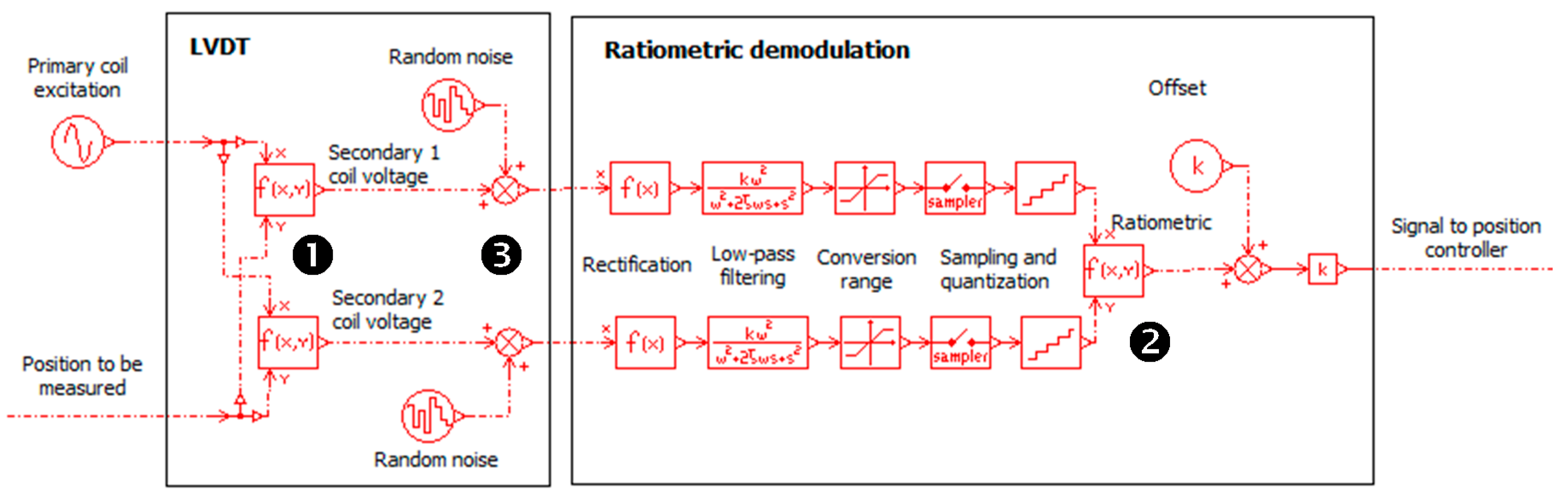
Common system-level models either do not introduce the dynamics and non-linearity of LVDT-based position sensing or focus too much on the sensor design itself—e.g., [34]. The proposed block diagram model is presented in Figure 18 A first block models the LVDT sensor itself, with its amplitude modulation operation. The two functions ❶ calculate the magnitude of the secondary voltages, according to the LVDT datasheet. The second block models the amplitude demodulation, the Analog-to-Digital Conversion (ADC), and the ratiometric calculation. ADC is performed at the position loop sampling frequency. The low pass filter that removes the high-frequency carrier is set to act as an anti-aliasing function at the sampling frequency. The ratiometric value is computed digitally in function ❷ as . A random noise is added in ❸. LVDTs are prone to bias that can reach 5% of the full scale for a 100 °C variation in temperature. Therefore, it becomes relevant to introduce the measurement offset. Of course, the LVDT can be modelled at a more detailed electrical level, including winding resistances, inductance, and flux linkage, if necessary. When the LVDT conditioning is performed by an integrated circuit—e.g., Analog Device AD598—its model parameterization can be facilitated by consulting the supplier’s datasheet.
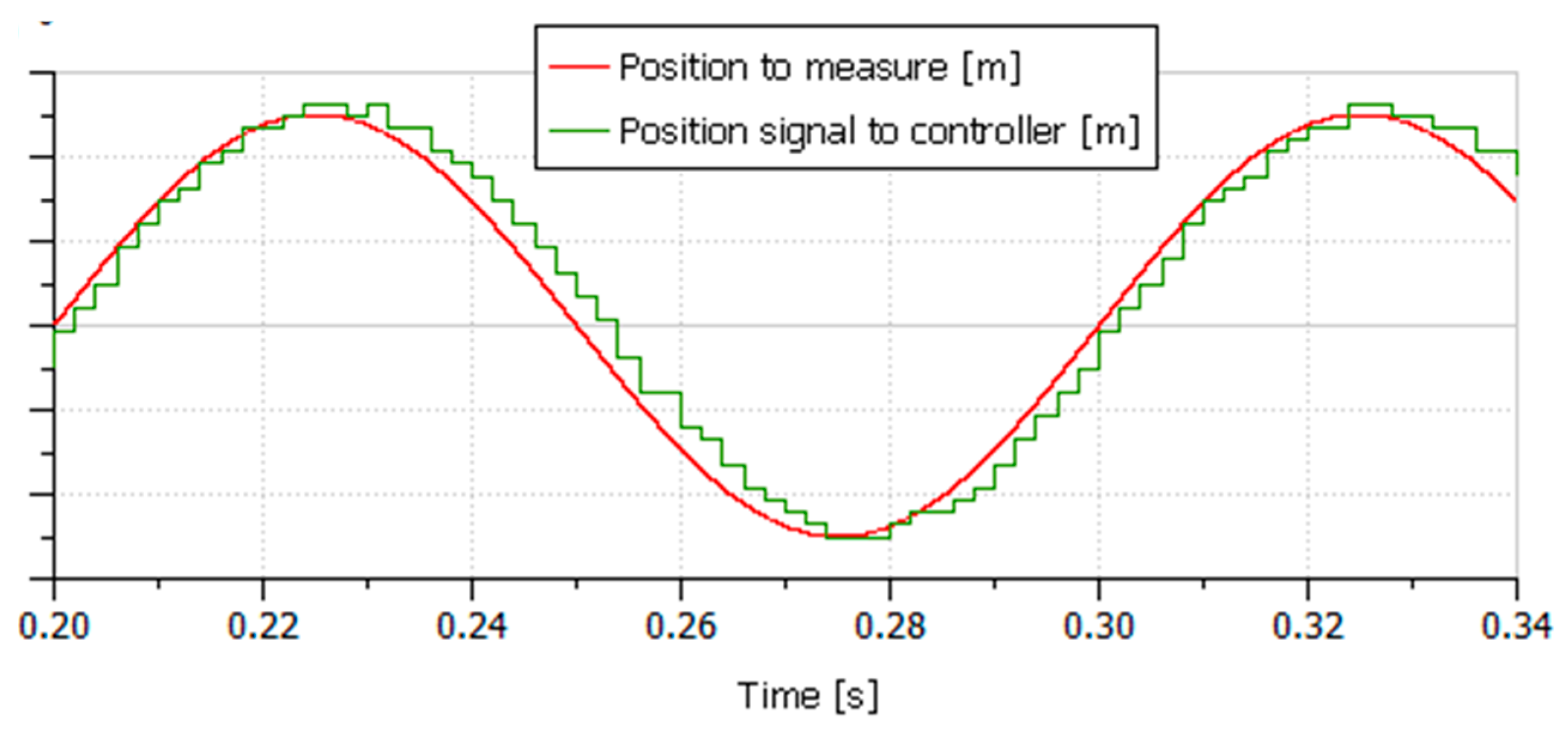
Figure 19 displays the quantization, sampling, and phase lag effects for the response of the position measurement chain. The rod position input frequency and magnitude are set according to the −3 dB performance test. The LVDT excitation frequency is 500 times the actuator bandwidth, and the sampling frequency is 50 times the actuator bandwidth. A 12-bit resolution is used, assuming ±2 LSB uniform noise and 16 LSB (0.4%) offset. The difference between the physical quantity and the value used for control feedback highlights the importance of modelling the measurement chain.
6.2.2. Rotor Position/Speed Measurement
As seen in Figure 2, the motor shaft angle and speed measurements contribute to numerous functions in the EMA. The speed signal not only provides the feedback signal for the EMA speed loop but is also used for the BEMF compensation of the current loop and for the determination of the current setpoint vs. the actual operating point when a flux weakening feature is implemented. Except in very specific sensor-less applications, the motor shaft angular position signal is needed to control the motor phase voltages according to the electric angle between the motor rotor and stator. Therefore, the rotor angle/speed measurement dynamics and resolution must be consistent with the expected performance of both the speed and current loops.
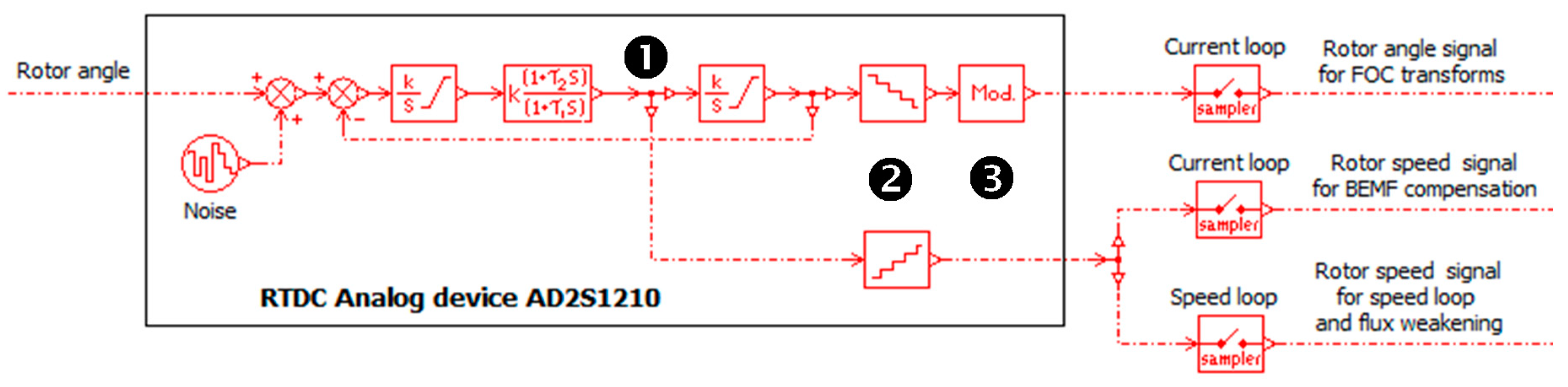
When high performance and reduced-torque ripple are required, EMA motors are controlled using an FOC approach. In this case, resolvers are seen as the best mature choice for rotor angle/speed measurement. However, for such a technology, the excitation, signal conditioning, and ADC become complex when a wide range of operation, high static accuracy, low tracking error, and high dynamics are expected. For this reason, chip manufacturers design off-the shelf programmable Resolver to Digital Converters RDC) to integrate these functions within a single physical unit: e.g., PGA411-Q1 from Texas Instruments (64 pins), AD2S1210 from Analog Devices (48 pins), or ACT5028B from Aeroflex (48 pins). Given the complexity of the circuit, the suppliers’ RDC datasheets usually provide a simplified dynamic model of the measurement chain. The following example of modelling applies to the AD2A1210 [35]. Simulating a full discrete model of the RDC would introduce numerous time events at the RDC operation frequency (e.g., 8.192 MHz). For this reason, a simplified continuous time domain model is implemented, as illustrated in Figure 20. In order to reduce the acceleration error, the RDC acts as a closed-loop double integrator system applied to the input angle to be measured. Stability of the loop is provided by a lead/lag filter ❶. The proposed model uses a specific parameter that enables the user to model the RDC setting (10-, 12-, 14-, and 16-bit resolution). Quantization ❷ of position and speed output, filter and loop gain parameters are set accordingly. The rotor angle is kept within one revolution range with a modulo function ❸. Position and speed signals are finally sampled according to the control function they serve. As for the position measurement, a noise of, e.g., ±2 LSB magnitude can to be added to increase the realism of the angle and the speed digital signals. For the virtual validation of the control design and actuator integration, it is not necessary to develop an electrical model of the resolver windings, although it does not raise any issues.
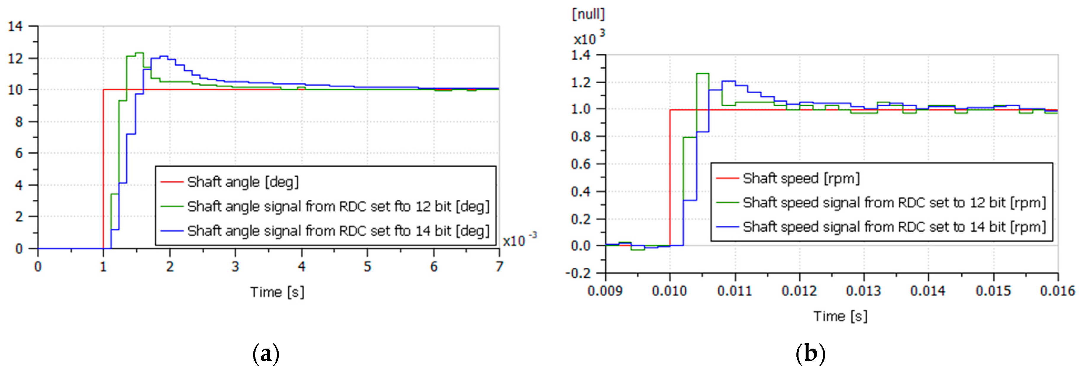
The response of the rotor angle/speed measurement chain is simulated, assuming that the RDC clock is set at the rated value of 8.192 MHz. The simulated responses are plotted in Figure 21. They give rise to the following comments that justify the interest of modelling the speed measurement chain realistically:
- For 12/14-bit resolutions, the overshoot of the speed measurement chain is 23%/21%, while the ±5% response time is 0.877/2.13 ms. Given these values, the RDC behaves globally as a second order system having a dimensionless damping factor of 0.45 and a natural frequency of 907/373 Hz. If the phase margin of the speed loop is measured at 100 Hz, the parasitic phase lag introduced by the 14-bit RDC at this frequency is 14.5°. This value is not negligible in comparison with the phase lag introduced by the equivalent delay of the speed loop sampling.
- The amount of quantization is verified with respect to the datasheet (0.088° and 176°/s for 12-bit configuration, 0.0217° and 21.6°/s for 14-bit configuration). For angle measurement, the 12-bit resolution could be acceptable for motors having a small number of pole pairs (e.g., the quantization error is 0.44° of the electric angle for five pole pairs). In contrast, the 12-bit resolution provides a very poor speed signal with a resolution of 146 rpm for the electric speed, even for a motor having five pole pairs. When the RDC model is integrated in the full model of the EMA, this poor resolution generates a high magnitude ripple on motor winding currents. This ripple is introduced at the current setpoint computed by the speed controller, the flux weakening function, and the BEMF compensation.
6.2.3. Current Measurement
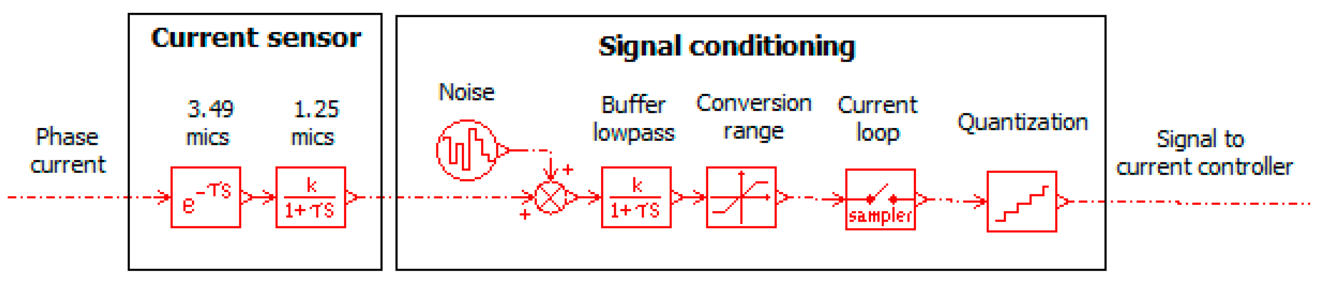
Current measurement is required to implement the winding current loops. The more straightforward method is to place current sensors in-line on the motor phase connections. Compared with shunt measurement, the Hall effect current sensors have become widely used because they accept a high common mode voltage, provide galvanic isolation between the power and signal lines, and can operate in DC conditions. Their main drawbacks (sensitivity and offset vs. temperature) have been significantly reduced with the newest generation. Electronic chip suppliers provide off-the-shelf bidirectional current-sensing eight-pin integrated circuits, all having a similar dynamic response: e.g., Melixis MLS91205, Texas Instruments TMCS1100, and Allegro ASC724. Again, the available models are generally devoted to the sensor design—e.g., [7]—and do not meet the needs of realistic system-level simulation. As shown by Figure 22, the simulation model developed for the current measurement chain includes:
- A model of the current sensor, identified from the ASC724 data sheet [36], which combines a pure delay of 3.49 μs and a first order lag of time constant 1.25 μs.
- A model of the signal conditioning that combines a buffer (also acting as an antialiasing filter), and the ADC (range limit, sampling, and quantization).
The response of the current measurement chain is given in Figure 23, with a current loop sampling frequency of 8 kHz, a buffer cut-off frequency of 4 kHz, and 12-bit resolution for ±5 A. As given by a formal calculation, the current-sensing chain introduces a total tracking delay of 44.4 μs. The current sensor dynamics contributes to only 10% of this value. Therefore, it is not a limiting factor to be considered during control design.
7. Conclusions
Several proposals have been made to increase the efficiency of MBD for EMAs. Being driven by needs and constraints, they provide practical considerations that come from experience feedback and lessons learnt in recent collaborative projects where scientists and industrialists worked together. Modelling and simulation have been addressed, with special consideration given to the process used for model development and its implementation for simulation. Multi-domain and multi-physics concern issues addressed simultaneously to provide proposals that have been successfully applied to various simulation platforms at both the signal- and power-chain levels. Proposals relative to motor and power electronics facilitate decision-making and avoid misleading parameterization. The suggested architecture of friction models potentially enables the main contributing phenomenon to be reproduced, while it conciliates scientists’ and engineers’ views. It has been shown how the proper modelling of controllers, sensors, and conditioners can provide useful criteria and means of assessment during preliminary design, sizing, and virtual verification or validation. The work is currently being extended to use simulation as a means to specify the real validation tests. The proposed models are consistent with the latest object-oriented concepts used for the structuring of the models’ libraries. This work also aims to contribute to the total removal of real tests, in favor of virtual tests, by increasing their acceptance by the regulatory authorities.
Funding
The reported work was funded by the Clean Sky 2 European project ASTIB (JTI-CS2-2014-CPW01-REG-01-01). This project aims at supporting the improvement of the Technological Readiness Level for a number of significant equipment items that are considered of critical importance for the future Green Regional Aircraft (GRA).
Acknowledgments
The author sincerely thanks the project partners for their constructive discussions during his development and implementation of EMA models.
Conflicts of Interest
The author declares no conflict of interest.
Abbreviations
| Acronyms | |
| ADC | Analog-To-Digital conversion |
| AW | Anti Windup |
| BEMF | Back ElectroMotive Force |
| EMA | ElectroMechanical Actuator |
| FOC | Field Oriented Control |
| IGBT | Insulated Gate Bipolar Transistor |
| LL | Line to Line |
| LN | Line to Neutral |
| LSB | Least Significant Bit |
| LVDT | Linear Variometer Differential Transducer |
| MBD | Model-Based Design |
| M&S | Modelling and Simulation |
| PI | Proportional-Integral |
| PMM | Property Model Methodology |
| PMSM | Permanent Magnet Synchronous Machine |
| PWM | Pulse Width Modulation |
| RDC | Resolver to Digital Converter |
| TRL | Technology Readiness Level |
| Nomenclature | |
| a, b, c | Phase labels (-) |
| f | Frequency (Hz) |
| F | Force (N) |
| I | Current (A) |
| J | Moment of inertia (kg·m2) |
| K | Gain (depends on context) |
| l | Lead (m/revolution) |
| L | Inductance (H) |
| m | Modulation factor (-) |
| p | Number of pole pairs (-) |
| P | Pressure (Pa) |
| P | Heat power (W) |
| R | Resistance (Ohm) |
| s | Laplace variable (s−1) |
| t | Time (s) |
| T | Torque (N.m) |
| V | Velocity (m/s) |
| x | Position (m) |
| X | General variable (depends on context) |
| U | Voltage (V) |
| ψ | Flux linkage (Wb) |
| ξ | Damping factor (-) |
| ω | Angular frequency (rad/s) |
| θ | Angular position (rad) |
| Ω | Angular velocity (rad/s) |
| τ | Time constant (s) |
| Θ | Temperature (°K) |
| ν | Kinematic viscosity (m2/s) |
| Subscript | |
| d | Direct axis, or drive |
| DC | Direct current |
| e | Equivalent |
| E | Electric |
| f | Force |
| i | Integral |
| I | Current |
| l | Limited, load |
| m | Motor |
| n | Natural, nut |
| r | Relative |
| rms | Root mean square |
| q | Quadrature axis |
| t | Transmission |
| T | Torque |
| x | Position |
| Ω | Velocity |
| Superscript | |
| * | Setpoint |
| ~ | Measure |
| ‘ | Maximal value in pseudo linear mode |
References
- SAE AE-7 Committee. Aerospace Information Report AIR6326: Aircraft Electrical Power Systems Modeling and Simulation Definitions; SAE: Warrendale, PA, USA, August 2015. [Google Scholar]
- Rose, L.M. The Application of Mathematical Modelling to Process Development and Design; Applied Science Publishers: London, UK, 1974; ISBN 0-85334-584-8. [Google Scholar]
- Van Der Linden, F.L.; Schlegel, C.; Christmann, M.; Regula, G.; Hill, C.; Giangrande, P.; Maré, J.-C.; Egaña, I. Implementation of a Modelica Library for Simulation of Electromechanical Actuators for Aircraft and Helicopters. In Proceedings of the 10th International Modelica Conference, Lund, Sweden, 10–12 March 2014; pp. 757–766. [Google Scholar]
- Rani, B.L.; Tom, A.M. Dynamic simulation of brushless DC drive considering phase commutation and backemf waveform for electromechanical actuator. In Proceedings of the TENCON 2008—2008 IEEE Region 10 Conference, Hyderabad, India, 19–21 November 2008; pp. 1–6. [Google Scholar]
- Bilyaletdinova, L.; Steblinkin, A. Simulation of Direct Drive Electromechanical Actuator with Ballscrew. Procedia Eng. 2017, 176, 85–95. [Google Scholar] [CrossRef]
- Byington, C.S.; Watson, M.; Edwards, D.; Stoelting, P. A model-based approach to prognostics and health management for flight control actuators. In Proceedings of the 2004 IEEE Aerospace Conference Proceedings (IEEE Cat. No.04TH8720), Big Sky, MT, USA, 6–13 March 2004; Volume 6, pp. 3551–3562. [Google Scholar] [CrossRef]
- Hill, C.; Gerada, C.; Giangrande, P.; Bozhko, S. Development of a Modelica Library for Electro-Mechanical, Actuator System Studies Including Fault Scenarios and Losses; SAE Technical Paper 2014-01-2181; SAE: Warrendale, PA, USA, 2014. [Google Scholar] [CrossRef]
- Şen, M.; Balabozov, J.; Yatchev, L.; Ivanov, R. Modelling of current sensor based on hall effect. In Proceedings of the 2017 15th International Conference on Electrical Machines, Drives and Power Systems (ELMA), Sofia, Bulgaria, 1–3 June 2017; pp. 457–460. [Google Scholar]
- Qiao, F.; Liu, Z. An Accurate Mathematic Model for PMSM by Taking Total Losses and Saturation into Account. Appl. Mech. Mater. 2015, 742, 505–510. [Google Scholar] [CrossRef]
- Micouin, P.; Fabre, L.; Becquet, R.; Paper, P.; Razafimahefa, T.; Guérin, F. Property Model Methodology: A Landing Gear Operational Use Case. In Proceedings of the INCOSE International Symposium 2018, Washington, DC, USA, 7–12 July 2018. [Google Scholar]
- Budinger, M.; Liscouët, J.; Maré, J.-C. Estimation models for the preliminary design of electromechanical actuators. Proc. Inst. Mech. Eng. Part G J. Aerosp. Eng. 2012, 226, 243–259. [Google Scholar] [CrossRef] [Green Version]
- Maré, J.-C. Requirement-based system-level simulation of mechanical transmissions with special consideration of friction, backlash and preload. Simul. Model. Pract. Theory 2016, 63, 58–82. [Google Scholar] [CrossRef]
- Takashi, M. The Effect of Tare Loss on the Efficiency of Mechanical Linear Actuators. Form Rev. N 2018. under revision. [Google Scholar]
- Akitani, S.; Bertolino, A. Increasing the fidelity of EMAs real-time simulation. In Proceedings of the SAE A-6 Symposium, Saint Pete Beach, FL, USA, 8 October 2019; Society of Automotive Engineers: Warrendale, PA, USA, 2019. [Google Scholar]
- Fu, J.; Maré, J.-C.; Yu, L.; Fu, Y. Multi-level virtual prototyping of electromechanical actuation system for more electric aircraft. Chin. J. Aeronaut. 2018, 31, 892–913. [Google Scholar] [CrossRef]
- Krykowski, K.; Hetmańczyk, J. Constant Current Models of Brushless DC Motor. Electr. Control. Commun. Eng. 2013, 3, 19–24. [Google Scholar] [CrossRef]
- Krishnan, R. Electric Motor Drives: Modeling, Analysis, and Control; Prentice Hall: Upper Saddle River, NJ, USA, 2001. [Google Scholar]
- Cai, H.; Dakai, H. On PMSM Model Fidelity and its Implementation in Simulation. In Proceedings of the IEEE Energy Conversion Congress and Exposition (ECCE) 2018, Portland, OR, USA, 23–27 September 2018; pp. 1674–1681. [Google Scholar] [CrossRef]
- Park, R.H. Two Reaction Theory of Synchronous Machines. In Transactions of the American Institute of Electrical Engineers. AIEE Trans. 1929, 48, 716–730. [Google Scholar] [CrossRef]
- Clarke, E. Circuit Analysis of A-C Power Systems, Vols. I and II. Stud. Q. J. 1951, 22, 95. [Google Scholar] [CrossRef]
- Krishnan, R. Permanent Magnet Synchronous and Brushless DC Motor Drives; Taylor and Francis Group: Boca Raton, FL, USA, 2010. [Google Scholar]
- Wu, T.; Bozhko, S.; Asher, G.; Wheeler, P.; Thomas, D. Fast Reduced Functional Models of Electromechanical Actuators for More-Electric Aircraft Power System Study; SAE Technical Paper 008-01-2859; SAE: Warrendale, PA, USA, 2008. [Google Scholar] [CrossRef]
- Maré, J.-C. Friction modelling and simulation at system level—Considerations to load and temperature effects. Proc. Inst. Mech. Eng. Part I J. Syst. Control Eng. 2014, 229, 27–48. [Google Scholar] [CrossRef]
- Hersey, M.D. The laws of lubrication of horizontal journal bearings. J. Wash. Acad. Sci. 1914, 4, 542–552. [Google Scholar]
- Aeroshell, Aerospace Grease 7, Technical Datasheet V1.1. 29 November 2014. Available online: https://www.shell.comwww.shell.com (accessed on 20 July 2020).
- The SKF Model for Calculating the Frictional Moment, SKF General Catalog 5000 E. 2003. Available online: https://www.skf.com (accessed on 20 July 2020).
- Olsson, H.; Åström, K.J.; de Wit, C.; Gäfvert, M.; Lischinsky, P. Friction Models and Friction Compensation. Eur. J. Control 1998, 4, 176–195. [Google Scholar] [CrossRef] [Green Version]
- Maré, J.-C. Friction modelling and simulation at system level: A practical view for the designer. Proc. Inst. Mech. Eng. Part I J. Syst. Control Eng. 2012, 226, 728–741. [Google Scholar] [CrossRef]
- Pennestri, E.; Rossi, V.; Salvini, P.; Valentini, P.P. Review and comparison of dry friction force models. Nonlinear Dyn. 2015, 83. [Google Scholar] [CrossRef]
- Modelica Association. Modelica®—A Unified Object-Oriented Language for Systems Modeling Language Specification; Version 3.4. 10 April 2017. Available online: https://www.modelica.org/documents/ModelicaSpec34.pdf (accessed on 25 September 2020).
- Coïc, C.; Fu, J.; Maré, J.-C. Bond Graphs Aided development of Mechanical Power Transmission for Aerospace Electromechanical Actuators. In Proceedings of the International Conference on Bond Graph Modeling and Simulation, Montreal, QC, Canada, 24–27 July 2016; pp. 221–228. [Google Scholar] [CrossRef]
- Maré, J.-C.; Akitani, S. Foundation for virtual prototyping of mechanical power management functions in electromechanical actuators. In Proceedings of the BATH/ASME FPMC Symposium on Fluid Power and Motion Control, Bath, UK, 12–14 September 2018. [Google Scholar] [CrossRef]
- Maré, J.-C. Aerospace Actuators—Volume 2: Signal-by-Wire and Power-by-Wire; ISTE/Wiley: London, UK, 2017. [Google Scholar]
- Drumea, A.; Svasta, P.; Blejan, M. Modelling and simulation of an inductive displacement sensor for mechatronic systems. In Proceedings of the 33rd International Spring Seminar on Electronics Technology, ISSE 2010, Warsaw, Poland, 12–16 May 2010; pp. 304–307. [Google Scholar] [CrossRef]
- Analog Devices, ADS1210 Datasheet Rev. A. 2010; p. 36. Available online: https://www.analog.com/media/en/technical-documentation/data-sheets/AD2S1210.pdf (accessed on 20 July 2020).
- ACS724LLCTR-20AB Current Sensor Datasheet, Allegro Microsystems ACS724-DS, Rev. 16. 3 April 2020. Available online: https://www.allegromicro.com (accessed on 20 July 2020).
Figure 1.
Example of an electromechanical unit for a flight control EMA.

Figure 2.
Example of the generic architecture of an EMA control unit (electromechanical unit partially shown).
Figure 2.
Example of the generic architecture of an EMA control unit (electromechanical unit partially shown).

Figure 3.
Image of the actuator studied in the frame of the Astib project, courtesy of Umbra.

Figure 4.
Top-level model of an EMA for the validation of EMA power and control specifications.

Figure 5.
Equivalent top-level model of the EMA when non-linear effects are neglected.

Figure 6.
Mapping of the dynamics in presence.

Figure 7.
Relations between the different expressions for PMSM constants (3-phase, star connection, power conservative d-q transform).
Figure 7.
Relations between the different expressions for PMSM constants (3-phase, star connection, power conservative d-q transform).

Figure 8.
PMSM equivalent model in the d-q frame: dq0 transform, non-salient poles.

Figure 9.
Equivalent DC motor model, usable for the dynamics, heat power, and power drawn from source.
Figure 9.
Equivalent DC motor model, usable for the dynamics, heat power, and power drawn from source.

Figure 10.
Compared responses of the full PMSM and equivalent DC motor models: (a) DC-bus currents and copper losses, (b) currents and airgap torques.
Figure 10.
Compared responses of the full PMSM and equivalent DC motor models: (a) DC-bus currents and copper losses, (b) currents and airgap torques.

Figure 11.
An example of the simplified DC-link model.

Figure 12.
Proposed generic architecture of a friction model (independent of the sticking/sliding transition management), (a) Bond-graph representation, (b) block-diagram representation.
Figure 12.
Proposed generic architecture of a friction model (independent of the sticking/sliding transition management), (a) Bond-graph representation, (b) block-diagram representation.

Figure 13.
Friction effects in a direct drive EMA (for aiding load, arrows are reversed).

Figure 14.
Proposed implementation of the friction model: (a) Bond-graph of the model structure, (b) implementation in Simcenter-Amesim.
Figure 14.
Proposed implementation of the friction model: (a) Bond-graph of the model structure, (b) implementation in Simcenter-Amesim.

Figure 15.
Compared timings for the update of PWM.

Figure 16.
An example of the PWM model implementation.

Figure 17.
Effect of the PWM realization on the current loop stability.

Figure 18.
Model of the position measurement chain.

Figure 19.
Response of the position measurement to a sine input.

Figure 20.
Model of the rotor/speed measurement chain made of a resolver and RDC.

Figure 21.
Dynamic response of RDC, (a) 10° step, (b) 1000 rpm step.

Figure 22.
Model of the current measurement chain model.

Figure 23.
Tracking error of the current measurement chain model.


Table 1.
Example of matrix for decision-making in modelling vs. engineering needs.
| Phenomenom Considered in the Model | Engineering Needs | Effects on Simulation | ||||||||||
|---|---|---|---|---|---|---|---|---|---|---|---|---|
| Functional | Power Sizing | Thermal Balance | Natural Dynamics | Closed-Loop Performance | Consumed/Regenerated Energy | Mechanical Load Propagation | Mode Switching /Response to Fault | Number of Parameters | Number ofState Variables | Time Scale | ||
| Control | ||||||||||||
| 1—Perfect (continuous, no saturation) | ||||||||||||
| 2—Discrete with saturations | ||||||||||||
| 3—Discrete with timing | ||||||||||||
| Sensors | ||||||||||||
| 1—Perfect (pure gain) | ||||||||||||
| 2—Plus accuracy, noise and dynamics | ||||||||||||
| 3—Plus detailed conditioning | ||||||||||||
| Power electronics | ||||||||||||
| 1—Perfect (modulated power transformer) | ||||||||||||
| 2—Basic (averaged, with efficiency) | ||||||||||||
| 3—Advanced (losses, heat, switched) | ||||||||||||
| Electric motor | ||||||||||||
| 1—Perfect (power transformer) | ||||||||||||
| 2—DC Equivalent (copper losses, inductance, inertia) | ||||||||||||
| 3—D-Q equivalent (copper losses, inductance, inertia) | ||||||||||||
| 4—3-phase, plus iron losses, cogging torque, cyclic L, saturation | ||||||||||||
| Mechanical transmission | ||||||||||||
| 1—Perfect (pure gain) | ||||||||||||
| 2—Plus inertia and simplified friction | ||||||||||||
| 3—Plus detailed friction, compliance and backlash | ||||||||||||
| 4—Plus multiple degrees of freedom | ||||||||||||
Table 2.
Recommended limits for the controller outputs.
| Controller | Practical Limit | Assumption and Comment |
|---|---|---|
| speed setpoint issued by the position controller. | Allowing the PWM to operate in the pseudo linear domain. | |
| and current demands issued by the speed controller and flux weakening function. | must be the max transient value permitted. | |
| and voltage demands issued by the current controllers. | Allowing the PWM to operate in the pseudo linear domain. In the simplest form, each and voltage is limited to . |
© 2020 by the author. Licensee MDPI, Basel, Switzerland. This article is an open access article distributed under the terms and conditions of the Creative Commons Attribution (CC BY) license (http://creativecommons.org/licenses/by/4.0/).
Share and Cite
MDPI and ACS Style
Maré, J.-C. Practical Considerations in the Modelling and Simulation of Electromechanical Actuators. Actuators 2020, 9, 94. https://0-doi-org.brum.beds.ac.uk/10.3390/act9040094
AMA Style
Maré J-C. Practical Considerations in the Modelling and Simulation of Electromechanical Actuators. Actuators. 2020; 9(4):94. https://0-doi-org.brum.beds.ac.uk/10.3390/act9040094
Chicago/Turabian StyleMaré, Jean-Charles. 2020. "Practical Considerations in the Modelling and Simulation of Electromechanical Actuators" Actuators 9, no. 4: 94. https://0-doi-org.brum.beds.ac.uk/10.3390/act9040094
Note that from the first issue of 2016, this journal uses article numbers instead of page numbers. See further details here.