An Alternative Empirical Model to Estimate Watershed Sediment Yield Based on Hydrology and Geomorphology of the Basin in Data-Scarce Rift Valley Lake Regions, Ethiopia

Abstract

Physical-based soil erosion models are playing an important role in the assessment of soil erosion, transportation, and deposition in the watershed. Most of these models were developed for data-rich areas of the world and they need a measured data to calibrate and validate their results. To apply such physical-based models, the main factor hindering is the lack of measured sediment data. The amount of sediment in the fluvial systems is the result of hydro-geomorphological processes of a watershed and the nature of stream flows. Therefore, this study aims to develop an alternative empirical model that generates the observed sediment data based on the hydro-geomorphology and nature of stream flows for Ziway Lake basin in the rift Valley of Ethiopia. By applying Soil and water Assessment Tool (SWAT), the lake basin was divided in to two sub-basins (Maki and Katar) with 26 of the watersheds within Maki. The SWAT model was calibrated and validated for both stream and sediment flow by using SUFI-2 program and its performance was assessed by using model evaluation statistics. With calibrated sediment flow rates of 26 Maki sub basins, an empirical model was developed by using its respective drainage area, average sub-basins slope, surface runoff, soil erodibility factor, stream flow rate, and average rive slopes. The applicability of the newly developed alternative model was tested by using model evaluation statistics and validated inside of Katar sub-basin. It is recommended to test the developed model in other basins to incorporate with SWAT CUP program to calibrate and validate the sediment yield at data scared area.

1. Introduction

Sediment erosion, transport, and deposition in fluvial systems are complex processes [1,2]. The erosion of soil particles from upland and deposition of sediment in low land area and banks of the river will depend on hydrology and geomorphology of a watershed [3]. Hydrologic parameters like rainfall depth, intensity, surface runoff, and stream flows will play a fundamental role in generation of the erosion and sediment transportation. Similarly, the production and transportation of sediment in the fluvial system will depends on watershed geomorphological parameters like drainage network (e.g., stream order, stream length, stream number, and bifurcation ratio), areal aspects of the drainage basin (e.g., length of overland flow, drainage density, and basin shape) and relief aspects (e.g., basin relief, relief ratio, ruggedness number, gradient ratio, basin slope, and relative relief) of the channel network and contributing ground slope [4,5].

An engineering technique used for determination of erosion rate of a watershed relies on two approaches: the upland watershed sediment yield predication approach and instream sediment predicating approach. In both methods, quantification of soil loss is one of the greatest challenges and to overcome its sophistication different models have been developed [1,2,6].

In different parts of the world, different upland watershed sediment yield quantification equations were developed. For example, Pacific Southwest Interagency Committee Method (PSIAC) [7], Universal Soil Loss Equation (USLE) [8], Modified Universal Soil Loss Equation (MUSLE) [9], Soil Loss Estimation Model for Southern Africa (SLEMSA) [10], Erosion Potential Method (EPM) [11], Sediment Delivery Distributed (SEDD) [12], Modular Soil Erosion System Project (MOSES) [13] and BQART [14] models have been used over many years. These models are developed for a specific area with the help of statistical observations based on parameters detected in the field [15]. Hence it may give fairly accurate results if the equation is applied to conditions similar to those from where the equation was derived.

To simulate and validate the sediment yield of the basin by mathematical and physical based distributed models, observed sediment data could be required. In most developing countries, unavailability of measured sediment data is restricting the applicability of such models. For sediment yield predication, a lot of empirical models are developed to predict the sediment yield either in the form of suspended or bed load. But all of them were developed by having laboratory analysis data on controlled environments. Hence, they can give an accurate result for the area where they were developed. Studies like [16,17] have criticized the methods due to having vastly different results from each other. In addition to this, they cannot be applied on data-scarce area like Ethiopia where the availability of sediment laboratory data is limited. Hence the formula that can account for the sediment yield without sophisticated (laboratory) data may be need for further sediment study. Therefore, the main objectives of this study is to develop an empirical model that can predict the sediment yield based with watershed hydrology and geomorphology. The Lake Ziway Basin is considered as a case study and the actual sediment rate of the basin is predicated by GIS-based watershed model, Soil and Water Assessment Tool (SWAT) through calibration and validation techniques.

2. Study Area

2.1. Location and Topography

Lake Ziway is located at the northern end of the southern Rift Valley (Figure 1). The lake is the shallowest lake in the country and drains to Lake Abiyata. It is the third largest freshwater lake of the Ethiopian Rift Valley lakes and the fourth in the country. The lake has a surface area of 423 km² and has five islands: namely Gelila, Debre Sina, Tulu Gudo, Tsedecha, and Fundro. The lake basin has a total area of 7285 km² and geographically it extends from 7°20′54″ to 8°25′56″ latitude and 38°13′02″ to 39°24′01″ longitude. The majority of the watershed is flat to gently undulating, but is bounded by a steep slope in the eastern and southeastern escarpments and is characterized by abrupt faults. There is a topographic difference of about 2600 m between the rift floor and the highland areas (mountains) of the basin.

2.2. Climate

The climate of the Lake Ziway basin is dry to sub-humid or humid. The lowland area surrounding the lake is arid or semi-arid, and the highlands are sub-dry humid to humid. The basin is classified into three main seasons based on its rainfall [18]. The long rainy season is summer and is locally known as Kiremt. The Kiremt rain represents 50–70% of the mean annual total rainfall. The dry period extends between October–February, locally known as Bega. The small rainy season, known as Belg, represents 20–30% of the annual rainfall and occurs from March–May.

There are twelve meteorological stations within and near the basin namely Arata, Bekoji SF, Ketera Genet, Kulumsa, Meraro, Ogolcho, Adamitulu, Bui, Butajra, Koshe, Maki, and Ziway; and their long term (1987–2016) mean annual rainfall ranges from 620 to 1225 mm. The areal map of rainfall depth by using the inverse distance square interpolation method (IDW) is shown in Figure 2.

2.3. Hydrology

The lake feeds by two main rivers Katar and Meki Rivers and over flow by Bulbula River to Lake Abiyata [19]. Katar River is the biggest perennial river starting from Arsi high lands (Kakka Mountain) and flowing towards the northwest and finally joins the lake. The river has a total watershed area of 3350 km². The watersheds of Katar River ascend to over 4256 masl on the summits of Chilalo and Kakka mountains. Consequently, the gradient of this river is generally steep throughout its course to Lake Ziway, and it is often deeply incised up to 50 m below the ground surface. Another feeder river Meki drains an area of 2433 km² from the Gurage Mountains to the west and northwest of Lake Ziway. Although the head water of Meki River is at an altitude of about 3500 masl, the river rapidly descends the rift valley escarpment to below 2000 m before being joined by several major tributaries, Meki River is incised in a steep-sided valley until it reaches Meki town at the head of its delta.

The entire outflow from Lake Ziway is through Bulbula River, which flows in the south direction to Lake Abiyata. Bulbula descends some 58 m over a distance of 30 km between Lake Ziway and Abiyata. In addition to surface out flow, there is a possibility for ground water flow from Lake Ziway to other central Main Ethiopian Rift Lakes: elevation of Lake Ziway is 1636 m, Langano 1585, Abiyata 1578 m, and Shalla 1550 m.

2.4. Geology, Soil and Land Use

The geology of Lake Ziway basin is divided into four major groups of rock units that are based on age-Precambrian to Early Paleozoic crystalline basement succession rock, Mesozoic sedimentary rock, Oligocene to middle Miocene pre-rift volcanic rock, and middle-Miocene to Holocene syn-and post-rift volcanic rock and unconsolidated sediments [20,21]. Reference [22] identified the most dominant six soil types namely: Andosols, Cambisols, Fluvisols Leptosols, Luvisols, and Vertisol. In the basin, agriculture has long history. The basin as a whole is a zone of intensive agricultural activity and different crops are grown in the region using both the kiremt (main rainy season consists June, July and August months) and belg (March, April and May) rains. For the basin’s total area, it is estimated that about 90% of the land is under different agricultural activities.

In the lake basin there have been dynamics land use changes [22], leading to extensive catchment degradation. Soil erosion, land degradation, and soil fertility decline are seen as a result of population pressure with the intensification of cultivation on productive land and increasing cultivation of more marginal lands, population growth, low levels of technology, and by improper land management systems in the basin [22].

3. Methodology

In the river basin, the sub-basin sediment yield can be obtained either by measuring each sub-basin’s outlet or by using a conceptual/physical model. Determining the sediment yield by measuring each sub basin outlet is the most preferred and trusted method, but it is not always practical; it is expensive and time consuming. To obtain the sediment yield of each sub basin with a limited measured sediment data, physically based models can be used. Physically based models can generate the sediment yields of each sub basin by using the sediment rating curve from limited gauging station with limited sets of measured data. Moreover, physically based models have the capability to classify the entire watershed into smaller sub basins. The Soil and Water Assessment Tool is one good example of a physically based model that can classify the basin in to sub basins and can model both gauged and ungauged parts of the basin. Hence, the model SWAT is selected to generate sediment data of the basin.

3.1. SWAT Model Development and Input Description

To develop the SWAT model, two types of dataset are required [23,24,25,26,27,28,29,30]. These are meteorological datasets and catchment characteristics datasets (topography (DEM), soil and land use maps) [31,32,33,34,35,36,37].

Hence, to set up the SWAT model for our study basin, 30 m by 30 m DEM, land use map, soil maps, and soil laboratory test results of the basin major soils types were obtained from the Ministry of Water Irrigation and Electricity of Ethiopia (MoWIE). Prior to the application of the data in the model, preprocessing work was carried out. The soil properties required to set up SWAT 2012 model are grain size percentage, soil texture, soil saturated hydraulic conductivity, soil available water, bulk density, and texture class. Therefore, these soil characteristics were obtained from laboratory test/analyzed result done under Rift valley lake basin Master Plan study document [22]. During the study of Rift Valley Lake Basin Master Plan, the soil samples were collected from all soil units of the basin and their physical and chemical laboratory analysis were conducted in the Ethiopia Water Works Design and supervision Enterprise laboratory. From out of 12 soil units of the basin, 203 soil samples were collected and its physical and chemical properties were analyzed. Hence, the soil data base of SWAT model is adjusted for the basin by using analyzed soil properties. The basins soil erodibility (K) factor was calculated using the equation of [38] from the analyzed soil parameters as follows:

$$\mathrm{KET}=0.34{\left[\left(\frac{\%\mathrm{Silt}}{\%\mathrm{Sand}+\%\mathrm{Clay}}\right)\times \frac{1}{\mathrm{BD}}\right]}^{0.33}\times 0.1317$$

(1)

where KET is soil erodibility factor by ton acre hour hundreds of acre⁻¹ foot⁻¹* tonf ⁻¹ inch⁻¹, % Silt, % Sand and % Clay are percentage of silt, sand and clay proportion in the soil respectively, BD = Bulk density of the soil (g.cm⁻³).

The meteorological data elements namely maximum and minimum temperature, daily precipitation, sunshine hours, wind speed, and relative humidity were obtained from thirty meteorological stations available within and nearby the study area. The stations record daily data of thrity one years (1987 to 2017) and were collected for the study. To fill the missing values of climate elements, weather generator model was used. The required statistical parameters were computed using the computer program developed by [39]. In the Lake Ziway basin, two meteorology stations namely Ziway and Bui have been analyzed and used to establish the weather generator database.

Lake Ziway has two major tributary rivers namely Katar and Meki and before joining to lake Ziway, there is a steam gauging station Maki along Maki river and Abura on Katar river. By using the stream flow gauging location of both rivers, in ArcGIS 10.2 with ArcWAT-2012 the spatial heterogeneity of lake sub-watersheds were delineated based on 30 by 30 m resolution DEM data. Accordingly, the entire study area has been divided into fifty-one sub-watersheds which are composed of twenty-six inside Maki and twenty-five inside of Katar Rivers sub-basins (Figure 3).

The model results were calibrated and validated by using historical stream flow and sediment flow data. The daily stream flow data was obtained from MoWIE and the sediment data was generated by using sediment–discharge rating curve developed by [40]. SWAT does not separate sediment load into suspended load and bed load, and the simulated total sediment load is supposed to include both. Hence, we assumed the bedload as 10% of suspended sediment load [19] that obtained from the rating curve and added for model calibration and validation. For Maki River, at Maki gauging station, the model was run for the simulation period of 1 January 1996 through December 2013. The stream flow and sediment data of ten years from 1999 to 2008 were used for calibration and the subsequent 5 years (2009–2013) were then used for the validation period. Similarly, For Katar River, the model was run for the period of 1987 to 2010 with 11 years (1990 to 2000) calibration and ten years (2001 to 2010) validation period. For both rivers, the first three years in the calibration run were used for model warm-up. Lastly, the model performance for fitting measured constituent data was evaluated by using four widely used statistics, namely R², NSE, RMSE and PBIAS, based on the value recommended by [41].

3.2. Identification of Geomorphological Parameters that Govern Sediment Yield

Soil erosion from highland areas and deposition of sediment in the low land area and banks of the river is primarily governed by geomorphology and hydrology of the basin. The geomorphology of a basin refers to its physical characteristics namely; area, slope, elongation ratio, shape factor, and hypsometric integral. Hence these parameters were detected by using SWAT-2012. For the parameters that could not be detected with the SWAT2012, GIS spatial analysis tools were used. By using the GIS spatial analysis tools, the maximum, and minimum as well as average elevation of each sub watershed was determined from the DEM of the area. The relief (R) value of the watershed was determined by using the formula developed by [5] and area, slope and watershed length parameters were obtained from the watershed configuration output data in SWAT2012. Sub-basin shape factors (Fs) and elongation ratios (Re) were calculated by using their respective formulas (

Table 1. Standard methods of morphometric parameters.

Morphometric Parameters	Methods and Descriptions	References
Stream length (SL)	Length of the stream	[42]
Elongation ratio (Re)	Re = 2/Lb*(A/π)1/2	[5]
Basin relief (Rb)	R = H-h; H is maximum elevation and h is minimum elevation within the basin	[5]
Basin Slope (S)	S = H/Lb,	[4]
Shape factor (Fs)	Fs = L2/A L is the length of the watershed; and A is the area of the watershed	[43]

).

To develop an alternative sediment predicating empirical formula, the interrelated sediment flow with basin hydro-geomorphological parameters was developed for Maki sub basin. Maki river basin was classified in to 26 sub basins and during SWAT calibration and validation (Figure 3). Hence the stream flow and sediment yield were extracted from calibrated SWAT2012 result. To evaluate the level of parameters (hydrologic and geomorphologic) dependence on the flow rates of the sediment, Pearson’s correlation statistics was carried out. Pearson’s correlation was applied by using SPSS statistical software to identify the most correlated factors.

Table 2. Pearson’s correlation matrix between sediment flow and different watershed parameters for the month July, 2010.

	SY	A	Sw	Re	Fs	SL	Sr	Q	K
Pearson Correlation	1	0.69 **	0.89 **	0.79 **	0.245	0.85 **	0.85 **	0.87 **	0.57 *
N	26	26	26	26	26	26	26	26	26

** Correlation is significant at the 0.01 level (2-tailed). * Correlation is significant at the 0.05 level (2-tailed). where SS = Sediment flow in 10³ ton/day in month July 2010, A is area m², Sw is Mean watershed slope (%), Reis Elongation ratio, Fs is Shape factor, SL is Stream length (m), Sr is Slope of the river (%), k is soil erodibility factor (t ha hr/ha MJ mm), and Q is Flow of each basin on month July (m³/s).

, shows the sample correlation result determined for the month July, 2010.

As shown in Table 2, the geomorphologic factors of watershed namely; area, slope, elongation ratio, and the hydrologic factor of stream discharge plays a great role in sediment outflow. Elongation ratio of the watershed determine the deposition rate of the sediment. In more elongated watershed, more sediment deposition will occur, if sufficient slope gradient is not available to drive the sediment load to the stream networks.

To develop the empirical formula that handles the sediment rate of the basin, the factors were classified in to two. Upland watershed factors that include the morphology (Table 2), surface run off, and soil erodibility rate of basin; and instream parameters that includes stream flow and stream average slope.

Surface runoff is a function of soil type, land cover, and rainfall amount of the basin. To predict this, Soil Conservation Service Curve Number (SCS-CN) model was used. The SCS-CN method computes direct runoff through an empirical equation that requires the rainfall and a watershed coefficient as inputs. The watershed coefficient is called as the curve number (CN), which represents the runoff potential of the land cover soil complex. Land use and treatment classes are used in the preparation of a hydrological soil-cover complex, which in turn is used in estimating direct runoff. The relation of land use, treatment and soil hydrological group is given in [44,45,46] for different types of land use.

Lastly, to predicate soil erodibility rate of the upper basin soil, the soil erodibility Equation (1) developed by [38] was used.

3.3. Model Development

The sediment yield of the watershed can be determined by using different watershed parameters, namely hydrologic and geomorphologic factors. To established an empirical model between sediment yield of the watershed and watershed parameters, DataFit model with the version of 9.0 was used. DataFit is a tool used to perform nonlinear regression (curve fitting), statistical analysis, and data plotting with up to 20 independent variables. The empirical formula between sediment yield (SY) and watershed geomorphological and hydrological parameters were determined using a nonlinear regression equation (Equation (2)) in DataFit model.

SY = function (geomorphology and hydrology)

(2)

Mathematically, the parameters in Equation (2) is equated as

$$\mathrm{SY}=X \left(Q_s^b\times A\times S_b\times K\right)+Y \left(q_r^d\times S_r\right),$$

(3)

where SY = sub basin sediment yield (tone/month). Q_s is Surface runoff (m³/s), A is area of each sub basin (km²), S_b is average slope of each sub basin (%), K is soil erodibility factor of the soil, q_r is stream flow (m³/s), S_r is average slope of the river (%), X and Y are constants from regression equation; and b and d are peak flow adjustment factors.

To develop the model, for each (26) sub basins, the values of CN, watershed slope, mean average rain fall, soil edibility rate, and drainage area were extracted by using Arc GIS 10.2. The mean monthly average rain fall was determined by using IDM from metrological gauging stations located near to the basin (Figure 2). The surface flow rate of each sun basin was calculated by using the CN method, the average slopes of the stream existing in the basin were calculated by extracting the elevation of the stream initial and end points from the DEM of the basin, and the length of the stream is measured in Arc GIS 10.2.

The newly developed alternative sediment yield predication model was tested and evaluated by two methods: namely using model evaluation statistics between predicted and observed values and validated by applying on another sub-basin. Statistically, it was evaluated by using four widely used model evaluation statistics: Namely, coefficient of determination (R²), Nash-Sutcliffe efficiency (NSE), root mean square error (RMSE) observations standard deviation ratio (RSR), and Percent bias (PBIAS) [41].

To validate the applicability of newly developed model, one of the sub basin of Lake Ziway Katar was used. Lake Ziway has two tributary rivers (Maki and Katar) and for both of them, the daily river flow rate was available in MoWIE and the daily sediment flow rate was determined by using a sediment rating curve developed for the sites by [40]. Hence, the empirical model developed for sub basin Maki was checked inside of the Karat sub-basin.

4. Results and Discussion

4.1. Curve Number of Lake Ziway Basin

From a hydrological point of view, the rainfall runoff relationship allows one to infer the hydrological behaviors of a watershed. Figure 4 presents the rainfall–runoff relationship for the Lake Ziway Basin based on an analysis of the hydrological database of the year 2010.

4.2. Determining Stream Flow and Sediment Data to Developed Alternative SSC Model

The sediment flow rate of the basin was determining by calibrating and validating the SWAT model for both sub basins (Maki and Katar). To obtain optimal fitting with the measured data, calibration was conducted manually and automatically by SUFI-2 program. The most sensitive parameters identified for both stations during calibration are SCS runoff curve number (CN2.mgt), saturated hydraulic conductivity (SOL_K.sol), effective hydraulic conductivity in main channel (CH_K2.rte), Ground water “revap” coefficient (GW_REVAP.gw), surface runoff lag time (SURLAG.bsn), available water capacity of the soil layer (mm H₂O/mm soil) (SOL_AWC.sol), threshold depth of water in the shallow aquifer required for return flow to occur (mm) (GWQMN.gw), Slope of watershed (HRU_SLP.hru), soil evaporation compensation factor (ESCO.hru), base flow alpha factor (days) (ALPHA_BF.gw), groundwater delay (days) (GW_DELAY.gw), Plant Evaporation Compensation Coefficient (EPCO), and moist bulk density (SOL_BD.sol) with different sensitivity ranks. The time serios of observed and predicated stream flow for Maki and Abura stations is shown in Figure 5 and Figure 6.

As shown in Figure 5 and Figure 6, for both gauging stations (Maki and Abura), calibration of the SWAT model has successfully achieved the measured daily stream flow. Similarly, during the validation stage, stream flow estimated by SWAT model is mimicked well for both stations.

The goodness-of-fit analysis of the calibration and validation stages of stream flows were determined as

Table 3. Daily streamflow calibration and validation model performance statistics.

Parameter	Maki Sub-Basin		Katar Sub-Basin
	Calibration	Validation	Calibration	Validation
NSE	0.73	0.71	0.79	0.85
R2	0.74	0.72	0.80	0.86
PBIAS	−10.8	15.78	12.12	13.97
RSR	0.52	0.54	0.45	0.39

and the SWAT developers [48] have recommend to accept calibration for hydrology at R² > 0.6, NSE > 0.5 and RSR < 0.7. Similarly, according to [41] recommendation, the model predicting ability is very good. Hence, the model stream flow result is acceptable to use for any further model development.

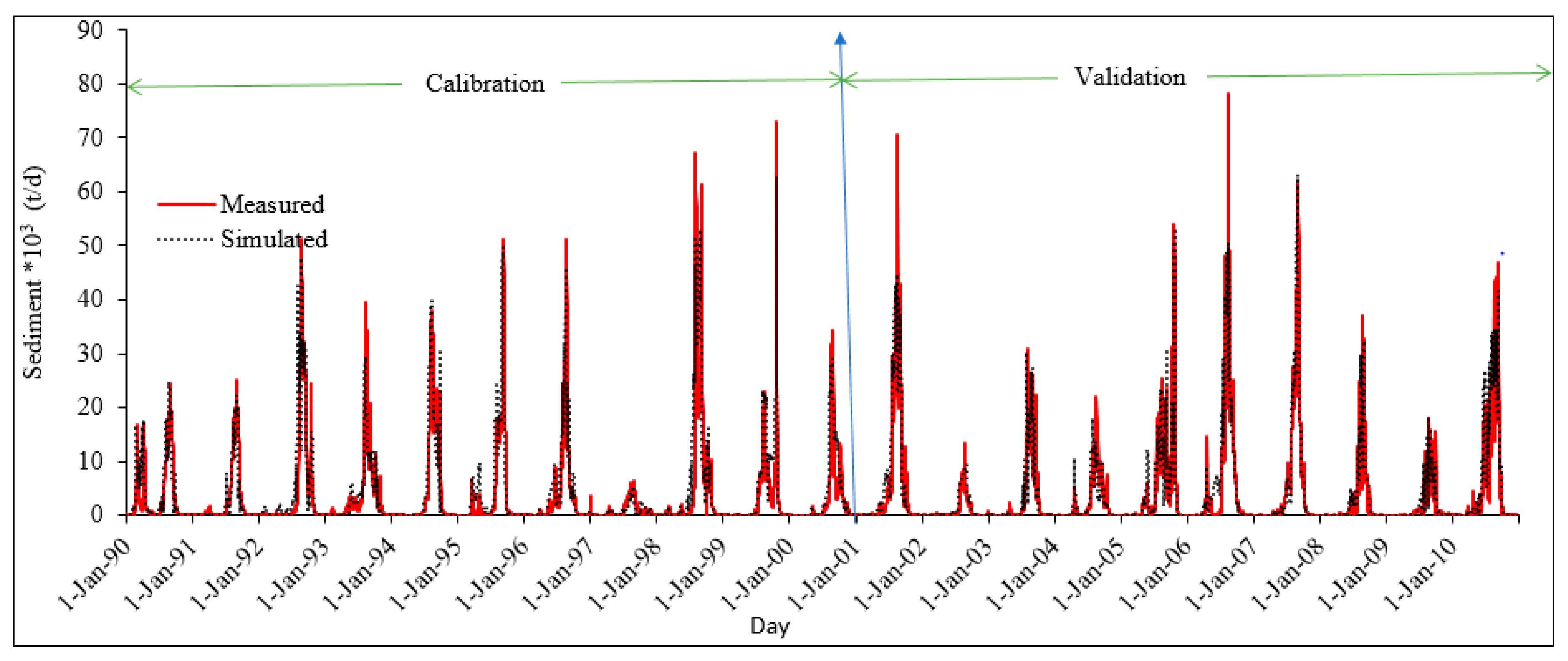
After steam flow calibrations, sediment flow calibration was done. In this celebration, six sensitive sediment parameters were identified. Those are USLE equation soil erodibility (K) factor, USLE support practice factor, Channel Erodibility factor, Linear factor for channel sediment routing, Exponential factor for channel sediment routing, and Channel Cover factor. The results of sediment calibration and validation of the sun basins are given in Figure 7 and Figure 8.

The calibrated and validation sediment results were verified as capable of simulating sediment yield as revealed by the statistical model efficiency criteria and is determined as

Table 4. Daily measured and simulated sediment yield calibration and validation model performance statistics.

Parameter	Maki Sun-Basin (At Station Maki)		Katar Sub-Basin (At Station Abura)
	Calibration	Validation	Calibration	Validation
NSE	0.74	0.75	0.72	0.77
R2	0.71	0.71	0.67	0.77
PBIAS	−7.87	−12.25	−16.68	−16.25
RSR	0.54	0.53	0.58	0.50

.

As can be seen in Table 4, all numerical model performance measures are in the acceptable range meaning that the SWAT model accurately tracked the measured sediment yields. Similarly, the graphical representation of measured and simulated flows matched well for both calibration and validation periods (Figure 7 and Figure 8). Hence, the result is confidentially used to develop an alternative empirical model that can substitute the measured data for the site.

4.3. Alternative Sediment Predication Model

By using the none linear regression method, an alternative sediment yield predication model is established by DataFit version 9.0 model as

$$\mathrm{SY}=0.04 \left(Q_s^b\times A\times S_b\times K\right)+0.07 \left(q_r^d\times S_r\right),$$

(4)

where SY is sub basin sediment yield (tone/month), Q_s is Surface runoff (m³/s), A is area of each sub basin (km²), S_b is average slope of each sub basin (%), K is soil erodibility factors of the soil, q_r is stream flow (m³/s), and S_r is average slope of the river (%).

In the model, b and d are peak flow adjustment factors. The value of b varies between 0.01 to 0.621 with mean value of 0.31072 and, d varies between 1.284 to 1.398 with mean value of 1.341. The selection of flow adjustment factors d and d are similar to the selection criteria of curve number. As the curve number CNI is recommended for dry seasons, the value of minimum d and b will be employed in such conditions of the seasons. Likewise, the curve number CNIII will be employed during rainy seasons. A similar approach is accepted for flow adjustment factors b and d. Hence in wet seasons the value of b and d will be 0.62144 and 1.3983401 respectively. For other normal seasons, the mean value of b and d will be employed.

4.4. Evaluation of the Newly Developed Model

4.4.1. Testing for Maki Sub-Basin

As the curve number varies from year to year due to change in land use, a single curve number cannot be employed for more than three to four years. The land used land cover change study in Katar sub basin of Lake Ziway by [49] indicates that there have been significant land use changes in the past two and half decades. According to their study, the dominant land use change was agriculture, with 27.7% between the year 1986 to 2010. As our curve number was developed for the year 2010, the evaluation of the model performance was employed only for three to four years before and after the year 2010.

The alternative model was developed in Maki sub basin by using geomorphological parameters of each 26 sub basins (Figure 3) and is tested for their common outlet point (Maki gauging station). For their common outlet point (gauging station Maki), the monthly sediment yield determined by an alternative empirical model and observed on the gauging station is shown in Figure 9.

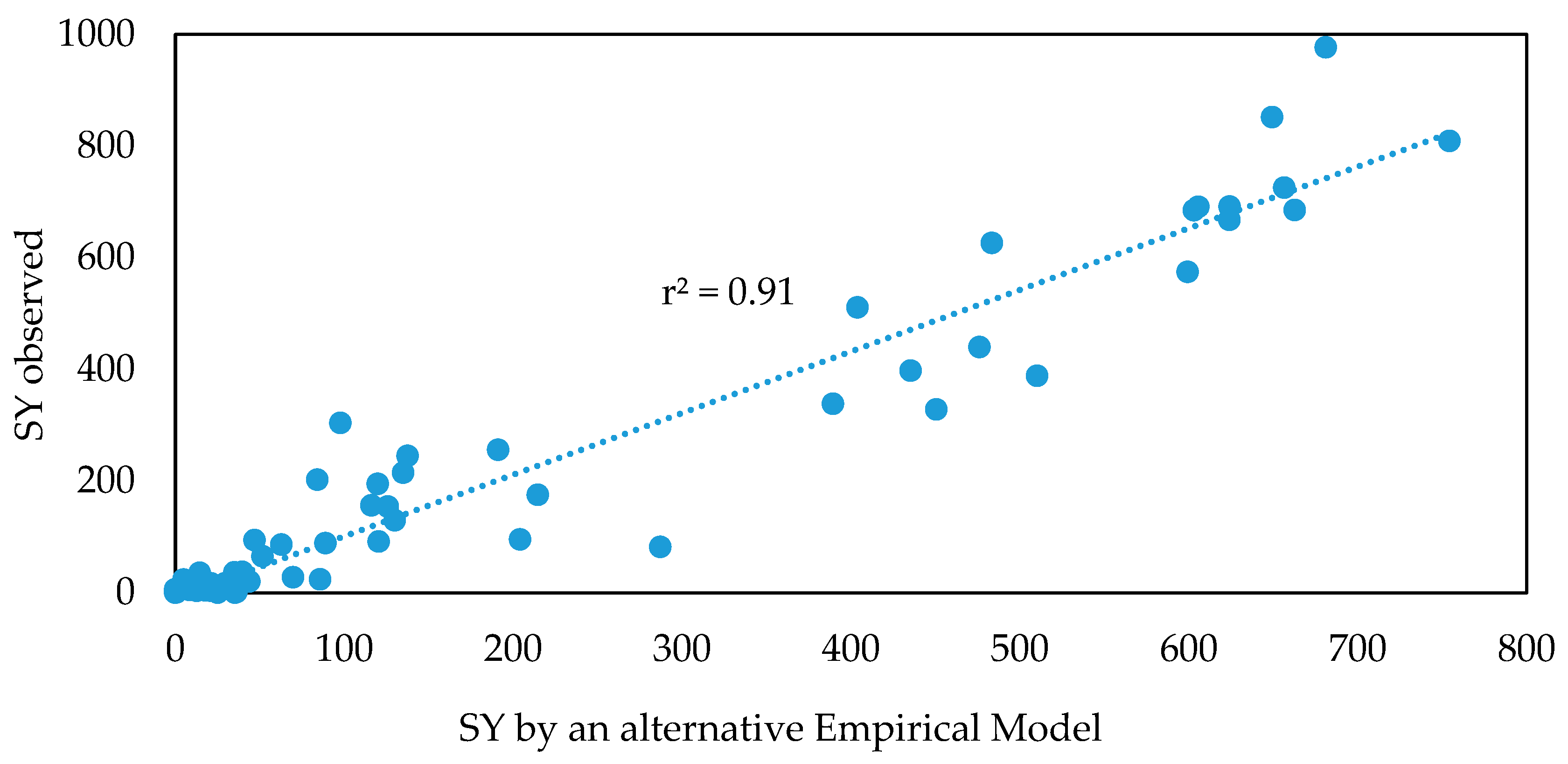
The time series plot of Figure 9 indicates that, the sediment yield observed and predicated by a newly developed alternative model matched well for both dry and wet seasons of the years. Similarly, the relation between the sediment flow rate determined by new empirical model and observe is shown in Figure 10 and well matches with each other.

As [41] demonstrated, if the R² Value is >0.9, 0.9 to 0.75, 0.65 to 0.75, and >0.50, the model can be rated as excellent, very good, adequate, and satisfactory performance, respectively. From Figure 8, it can be observed that the alternative sediment predication performance is excellent (R² = 0.905). Additional numerical criteria of model performance evaluators, namely NSE, RSR, and PBIAS, are determined and summarized in

Table 5. Statistics values for model performance.

Statistics	R2	NSE	RSR	PBIAS
Statistics values	0.91	0.90	0.33	4.95

.

As recommended by [41], the high R² and NSE (above 0.9) values and the reasonably low RSR (below 0.5) and PBIAS (below 5) indicate the excellent correlation and agreement between developed alternative sediment estimation model and observed one. As shown in Table 5, for all statistical evaluators, the performance of newly developed model is excellent.

4.4.2. Evaluating the Model Performance Inside of Kata Sub Basin

The Katar, one of the sub basin of Lake Ziway was used to evaluate the model performance. The sub basin has a drainage area of 3225 km² on the stream gauging station of Abura. The sub basin was divided in to 25 Sub basins during SWAT model calibration. The newly developed alternative sediment estimation model has been used to compute the sediment outflow from the total basin. The computed monthly sediment yield determined by an alternative empirical model and observed in stream gauging station Abura is shown in Figure 11.

The time series plot (Figure 11), that indicated the ration between an observed monthly sediment concentration and that predicated in an alternative model indicates as it has well matched for both dry and wet seasons of the years. Similarly, the relation between the sediment flow rate determined by new empirical model and observed in the gauging station Abura is shown in Figure 12 and well matches with each other.

Additional numerical criteria of model performance evaluators namely: NSE, RSR and PBIAS are determined and summarized in

Table 6. Statistics values for model performance.

Statistics	R2	NSE	RSR	PBIAS
Statistics values	0.89	0.83	0.46	−30.28

. As recommended by [41], the high R² and NSE values and the reasonably low RSR and PBIAS indicate the excellent correlation and agreement between data generated by an alternative model and observed one. As shown in Table 6, the performance of newly developed model is very good to excellent.

4.5. Some of the Unique Difference of the Newly Developed Model from the Existing Once

In soil erosion predication methods, the USLE has a long story. The modified of USLE was also derived by [50] and it can be used to estimate sediment yield in a catchment. In different parts of the world, the MUSLE has been applied to estimated the sediment yields of the basins both from agricultural and non-agricultural lands. Moreover, in computer based simulated models like SWAT, the equation has been used to analysis the sediment yields of basins and sub basins [51]. Here, the newly developed model has some similarity with USLE model. Like that of USLE, it accounts the effect of rain fall, soil, land use and slopes of the watershed. Unlike to that of USLE model, it accounts for the impacts of stream flow conditions on sediment transportation. Both the detachment and transport limited forms of erosion can be assessed in this method.

In northern Ethiopia, [52] developed the model that can estimate the sediment yield of the watershed. The developed mode by [52] is shown as

$$LogSY=0.007\times SBCG+0.003\times ELL+0.002\times RG-0.007\times BUSH+2.33$$

(5)

where, Log SY is sediment yield in t km⁻² yr⁻¹, SBCG is standard bank collapse and gully erosion, EL is proportion of erodibility lithology in %, RG is surface roughness, and BUSH is proportion of bush or shrub cover in %.

As shown in Equation (5), the effect of climate parameters was not explicitly included. As indicated in USLE and on its derivatives, climate is one of the major factors that govern the watershed sediment flow. In the discussion parts of the investigation, [52] pointed out the need for further analysis to obtain a good sediment predication model by incorporating climatic factors of the watershed. Hence, this study may answer the drown back seen on previous studies.

5. Conclusions

The newly developed an alternative watershed sediment yield estimation model was developed by using the geomorphologic, hydrologic, and hydraulic parameters of the watershed. It was developed based on an assumption that the sediment delivered on the outlet of the basin is originated from the upland area of the basin and from the section of stream channel. Basin area, slope, soil erodibility rate, and surface runoff were used as a component that govern the sediment yield on uplands of the basin. Similarly, stream channel slope and rate of stream flow was taken as a component that govern the sediment yield instream.

An alternative sediment predication model was developed in side of Maki sub basin of Lake Ziway and its performance was tested by using commonly used model evaluation statistics, namely coefficient of determination (R²), Nash-Sutcliffe efficiency (NSE), root mean square error (RMSE), observations standard deviation ratio (RSR), and Percent bias (PBIAS). The applicability of the model for other basins was also tested by using the Katar sub basin as a case study. Hence, its applicability was validated in Katar sub basin. Statistically, the performance of the model inside of Maki sub basin is excellent, and during validation, the newly developed model performance is excellent to very good.

The model was also tested by plotting the time-series graphs of sediment estimated by the newly developed model and measured one. The result indicates that an alternative model is duplicating the sediment yield measured in the gauging stations. To apply a physical based model such as SWAT, the main factor hindering it is the lack of measured sediment data. For the study area, the developed model is a solution for such problems. Lastly, we would like to recommend that, this the newly developed model has to be tested in other basins to incorporate with SWAT CUP program to calibrate and validate the sediment yield at data scared area.

References

- Arekhi, S.; Niazi, Y.; Kalteh, A.M. Soil erosion and sediment yield modeling using RS and GIS techniques: A case study, Iran. Arab. J. Geosci. 2010, 5, 285–296. [Google Scholar] [CrossRef]
- Salsabilla, A.; Kusratmoko, E. Assessment of Soil Erosion Risk in Komering Watershed, South Sumatera, Using SWAT Model. In AIP Conference Proceedings; American Institute of Physics: College Park, MD, USA, 2017; Volume 1862. [Google Scholar]
- Marttila, H.; Kløve, B. Dynamics of erosion and suspended sediment transport from drained peatland forestry. J. Hydrol. 2010, 388, 414–425. [Google Scholar] [CrossRef]
- Miller, V.C. Quantitative Geomorphic Study of Drainage Basin Characteristics in the Clinch Mountain Area, Virginia and Tennessee; Technical report (Columbia University. Department of Geology) No. 3 1953; Department of Geology, Columbia University: New York, NY, USA, 2014. [Google Scholar]
- Schumm, S.A. Evolution of Drainage Systems and Slopes in Badlands at Perth Amboy, New Jersey. GSA Bull. 1956, 67, 597–646. [Google Scholar] [CrossRef]
- Boggs, G.; Devonport, C.; Evans, K.; Puig, P. GIS-based rapid assessment of erosion risk in a small catchment in a wet/dry tropic of Australia. Land Degrad. Dev. 2001, 12, 417–434. [Google Scholar] [CrossRef]
- PSIAC Factors Affecting Sediment Yield and Measures for the Reduction of Erosion and Sediment Yield; Pacific Southwest Inter-Agency Committee: San Francisco, CA, USA, 1996.
- Wischmeier, W.H.; Smith, D.D. Predicting Rainfall Erosion Losses—A Guide to Conservation Planning; USDA, Science and Education Administration: Hyattsville, MA, USA, 1978; pp. 537–539.
- Williams, J.R.; Berndt, H.D. Sediment Yield Prediction Based on Watershed Hydrology. Trans. ASAE 1977, 20, 1100–1104. [Google Scholar] [CrossRef]
- Stocking, M.A. Working Model for the Estimation of Soil Loss Suitable for Underdeveloped Areas; School of Development Studies, University of East Anglia: Norwich, UK, 1981. [Google Scholar]
- Nearing, M.A.; Simanton, J.R.; Norton, L.D.; Bulygin, S.J.; Stone, J. Soil erosion by surface water flow on a stony, semiarid hillslope. Earth Surf. Process. Land. 1999, 24, 677–686. [Google Scholar] [CrossRef]
- Ferro, V.; Porto, P. Sediment Delivery Distributed (SEDD) Model. J. Hydrol. Eng. 2000, 5, 411–422. [Google Scholar] [CrossRef]
- Meyer, C.R.; Wagner, L.E.; Yoder, D.C.; Flanagan, D.C. The modular soil erosion system (MOSES). In Soil Erosion; American Society of Agricultural and Biological Engineers: St. Joseph, MI, USA, 2001; p. 358. [Google Scholar]
- Syvitski, J.P.M.; Milliman, J.D. Geology, Geography, and Humans Battle for Dominance over the Delivery of Fluvial Sediment to the Coastal Ocean. J. Geol. 2007, 115, 1–19. [Google Scholar] [CrossRef] [Green Version]
- Hajigholizadeh, M.; Melesse, A.M.; Fuentes, H.R. Erosion and Sediment Transport Modelling in Shallow Waters: A Review on Approaches, Models and Applications. Int. J. Environ. Res. Public Health 2018, 15, 518. [Google Scholar] [CrossRef] [Green Version]
- Yang, C.T. Unit Stream Power Equation for Gravel. J. Hydraul. Eng. 1984, 110, 1783–1797. [Google Scholar] [CrossRef]
- Yang, C.T. Sediment Transport Theory and Practice; Krieger Publishing Company: Malabar, FL, USA, 2003. [Google Scholar]
- Legesse, D. Analysis of the Hydrological Response of the Ziway–Shala Lake Basin (Main Ethiopian Rift) to Changes in Climate and Human Activities. Ph.D. Thesis, University d’Aix-Marseille III, Aix-en-Provenece, France, 2002. [Google Scholar]
- Aga, A.O.; Chane, B.; Melesse, A.M. Soil Erosion Modelling and Risk Assessment in Data Scarce Rift Valley Lake Regions, Ethiopia. Water 2018, 10, 1684. [Google Scholar] [CrossRef] [Green Version]
- Ayenew, T. The Hydrogeological System of the Lake District Basin: Central Main Ethiopian Rift; ITC: Enschede, The Netherlands, 1998. [Google Scholar]
- Makin, M.J.; Kingham, T.J.; Waddams, A.E.; Birchall, C.J.; Eavis, B.W. Prospects for Irrigation Development around Lake Zwai, Ethiopia; Land Resources Division, Ministry of Overseas Development: Surrey, UK, 1976.
- Halcrow, G. Rift Valley Lakes Basin Integrated Resources Development Master Plan Study Project; The Federal Democratic Republic of Ethiopia-Ministry of Water Resources (MOWR): Addis Ababa, Ethiopia, 2010.
- Dessu, S.B.; Melesse, A.M.; Bhat, M.G.; McClain, M.E. Assessment of water resources availability and demand in the Mara River Basin. Catena 2014, 115, 104–114. [Google Scholar] [CrossRef]
- Dessu, S.; Melesse, A.M. Modelling the rainfall–runoff process ofthe Mara River basin using the soil and water assessment tool. Hydrol. Process. 2012, 26, 4038–4049. [Google Scholar] [CrossRef]
- Dessu, S.; Melesse, A.M. Impact and uncertainties of climate change on the hydrology of the Mara River basin, Kenya/Tanzania. Hydrol. Process. 2013, 27, 2973–2986. [Google Scholar] [CrossRef]
- Setegn, S.G.; Dargahi, B.; Srinivasan, R.; Melesse, A.M. Modeling of Sediment Yield from Anjeni-Gauged Watershed, Ethiopia Using SWAT Model. JAWRA J. Am. Water Resour. Assoc. 2010, 46, 514–526. [Google Scholar] [CrossRef]
- Setegn, S.G.; Srinivasan, R.; Dargahi, B.; Melesse, A.M. Spatial delineation of soil erosion vulnerability in the Lake Tana Basin, Ethiopia. Hydrol. Process. 2009, 23, 3738–3750. [Google Scholar] [CrossRef]
- Setegn, S.G.; Rayner, D.; Melesse, A.M.; Dargahi, B.; Srinivasan, R. Impact of climate change on the Hydroclimatology of Lake Tana Basin, Ethiopia. Water Resour. Res. 2011, 47, W04511. [Google Scholar] [CrossRef]
- Setegn, S.G.; Srinivasan, R.; Melesse, A.M.; Dargahi, B. SWAT model application and prediction uncertainty analysis in the Lake Tana Basin, Ethiopia. Hydrol. Process. 2010, 24, 357–367. [Google Scholar] [CrossRef]
- Yesuf, H.M.; Assen, M.; Alamirew, T.; Melesse, A.M. Modeling of sediment yield in Maybar gauged watershed using SWAT, northeast Ethiopia. Catena 2015, 127, 191–205. [Google Scholar] [CrossRef]
- Grey, O.; Webber, D.F.S.G.; Setegn, S.; Melesse, A.M. Application of the soil and water assessment tool (SWAT model) on a small tropical island (Great River watershed, Jamaica) as a tool in integrated watershed and coastal zone management. Int. J. Trop. Biol. Conserv. 2014, 62, 293–305. [Google Scholar]
- Maalim, F.K.; Melesse, A.M. Modelling the impacts of subsurface drainage on surface runoff and sediment yield in the Le Sueur Watershed, Minnesota, USA. Hydrol. Sci. J. 2013, 58, 570–586. [Google Scholar] [CrossRef] [Green Version]
- Mekonnen, M.; Melesse, A.M. Soil Erosion Mapping and Hotspot Area Identification Using GIS and Remote Sensing in Northwest Ethiopian Highlands, Near Lake Tana. In Nile River Basin; Springer: Dordrecht, The Netherlands, 2011; pp. 207–224. ISBN 978-94-007-0688-0. [Google Scholar]
- Wang, X.; Garza, J.; Whitney, M.; Melesse, A.; Yang, W. Prediction of Sediment Source Areas within Watersheds as Affected by Soil Data Resolution. In Environmental Modelling; Nova Science Publishers Inc., Hauppauge: New York, NY, USA, 2008; pp. 151–185. [Google Scholar]
- Hunink, J.; Niadas, I.; Antonaropoulos, P.; Droogers, P.; De Vente, J. Targeting of intervention areas to reduce reservoir sedimentation in the Tana catchment (Kenya) using SWAT. Hydrol. Sci. J. 2013, 58, 600–614. [Google Scholar] [CrossRef] [Green Version]
- Msaghaa, J.J.; Melesse, A.M.; Ndomba, P.M. Modeling Sediment Dynamics: Effect of Land Use, Topography, and Land Management in the Wami-Ruvu Basin, Tanzania. In Nile River Basin; Springer: Cham, Switzerland, 2014; pp. 165–192. ISBN 978-3-319-02719-7. [Google Scholar]
- Msaghaa, J.J. Sediment Yield Modeling and Dentification of Erosion Hotspots in Tropical Watersheds: The Case of Upper Ruvu Catchment in Tanzania. Master’s Thesis, Florida International University, Miami, FL, USA, 2012. [Google Scholar]
- Aga, A.O.; Melesse, A.M.; Chane, B. An alternative soil erodibility estimation approach for data scarce regions: A case of Ethiopian Rift Valley Lake Basin. J. Arid Land 2019, in press. [Google Scholar]
- Liersch, S. The Program pcpSTAT User’s Manual. 2003. Available online: http://www.brc.tamus.edu/swat/pcpSTAT.zip (accessed on 12 August 2003).
- Aga, A.O.; Melesse, A.M.; Chane, B. Estimating the Sediment Flux and Budget for a Data Limited Rift Valley Lake in Ethiopia. Hydrology 2019, 6, 1. [Google Scholar] [CrossRef] [Green Version]
- Moriasi, D.N.; Arnold, J.G.; Van Liew, M.W.; Bingner, R.L.; Harmel, R.D.; Veith, T.L. Model Evaluation Guidelines for Systematic Quantification of Accuracy in Watershed Simulations. Trans. ASABE 2007, 50, 885–900. [Google Scholar] [CrossRef]
- Horton, R.E. Erosional Development of Streams and Their Drainage Basins.; Hydrophysical Approach to Quantitative Morphology. GSA Bull. 1945, 56, 275. [Google Scholar] [CrossRef] [Green Version]
- Horton, R.E. Drainage-basin characteristics. EOS Trans. Am. Geophys. Union 1932, 13, 350–361. [Google Scholar] [CrossRef]
- Melesse, A.M.; Graham, W.D.; Jordan, J.D. Spatially Distributed Watershed Mapping and Modeling: GIS-based Storm Runoff and Hydrograph Analysis: (Part 2). J. Spat. Hydrol. 2003, 3, 2. [Google Scholar]
- USDA Soil Conservation Service. National Engineering Handbook, Section 4, Hydrology; USDA Soil Conservation Service: Washington, DC, USA, 1972.
- USDA Natural Resource Conservation Service. National Engineering Handbook—Part Chapter 9: Hydrologic Soil Cover Complexes; USDA Natural Resource Conservation Service: Washington, DC, USA, 2004.
- Chow, V.T.; Maidment, K.D.; Mays, L.W. Applied Hydrology; McGrow-Hill Book Company: New York, NY, USA, 2002. [Google Scholar]
- Santhi, C.; Arnold, J.; Williams, J.R.; Dugas, W.A.; Srinivasan, R.; Hauck, L.M. Validation of the SWAT model on a large river basin with point and nonpoint sources. J. Am. Water Resour. Assoc. 2001, 37, 1169–1188. [Google Scholar] [CrossRef]
- Tufa, D.F.; Abbulu, Y.; Rao, G.V.R. Hydrological impacts Due to land-use and land-cover changes of Ketar watershed, Lake Ziway catchment, Ethiopia. Int. J. Civ. Eng. Technol. 2015, 6, 36–45. [Google Scholar]
- Williams, J. Sediment-yield prediction with Universal Equation using runoff energy factor. In Present and Prospective Technology for Predicting Sediment Yield and Sources; U.S. Department of Agriculture: Washington, DC, USA, 1975; Volume ARS-S-40, pp. 244–252. [Google Scholar]
- Arnold, J.G.; Williams, J.R.; Maidment, D.R. Continuous-Time Water and Sediment-Routing Model for Large Basins. J. Hydraul. Eng. 1995, 121, 171–183. [Google Scholar] [CrossRef]
- Tamene, L.; Park, S.J.; Dikau, R.; Vlek, P.L.G. Reservoir siltation in the semi-arid highlands of northern Ethiopia: Sediment yield–catchment area relationship and a semi-quantitative approach for predicting sediment yield. Earth Surf. Process. Land. 2006, 31, 1364–1383. [Google Scholar] [CrossRef]
© 2020 by the authors. Licensee MDPI, Basel, Switzerland. This article is an open access article distributed under the terms and conditions of the Creative Commons Attribution (CC BY) license (http://creativecommons.org/licenses/by/4.0/).