The Impact of Quality of Digital Elevation Models on the Result of Landslide Susceptibility Modeling Using the Method of Weights of Evidence

Abstract
:1. Introduction
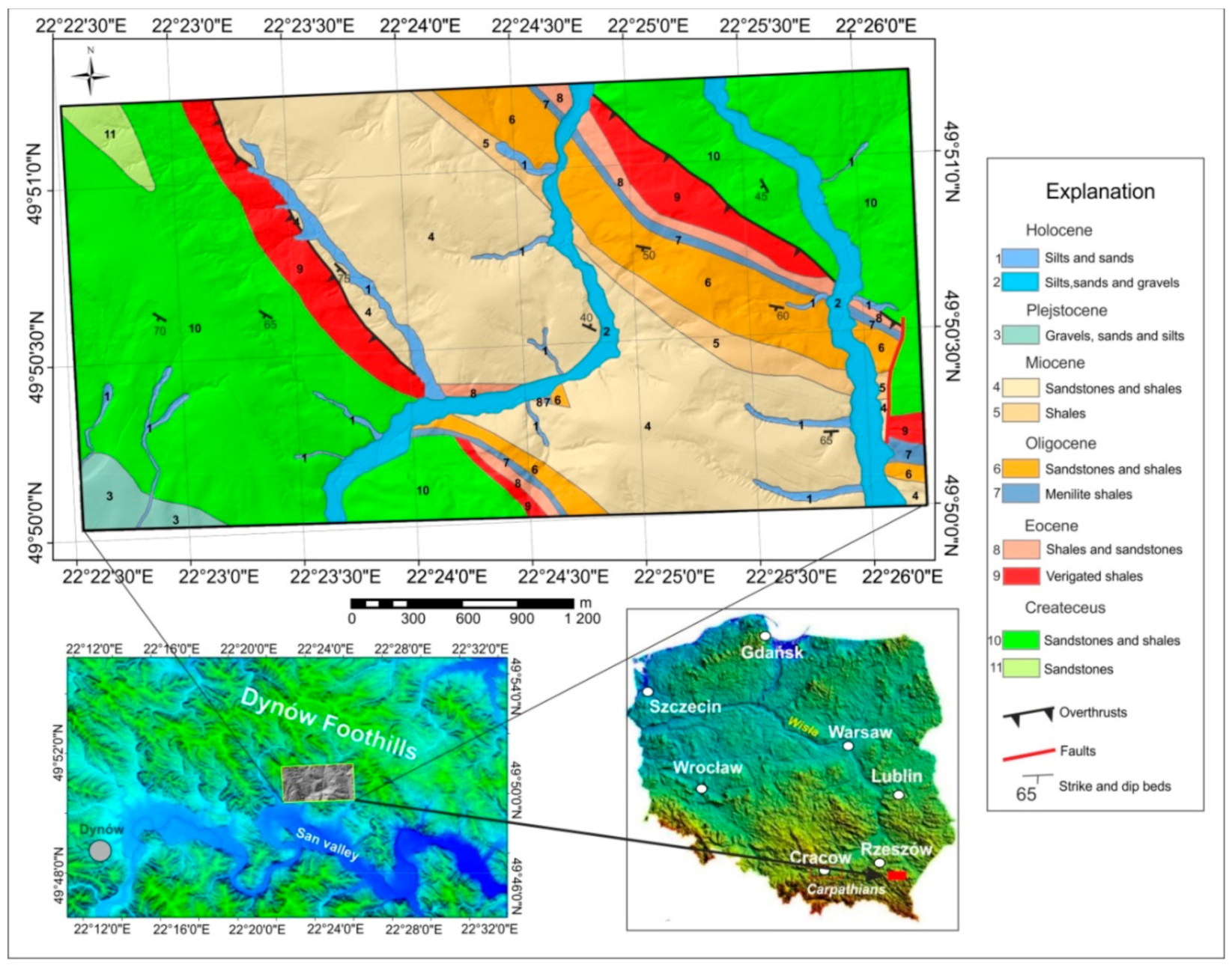
2. Study Area
3. Methods and Materials
3.1. Archival Digital Stereo-Pair Aerial Images
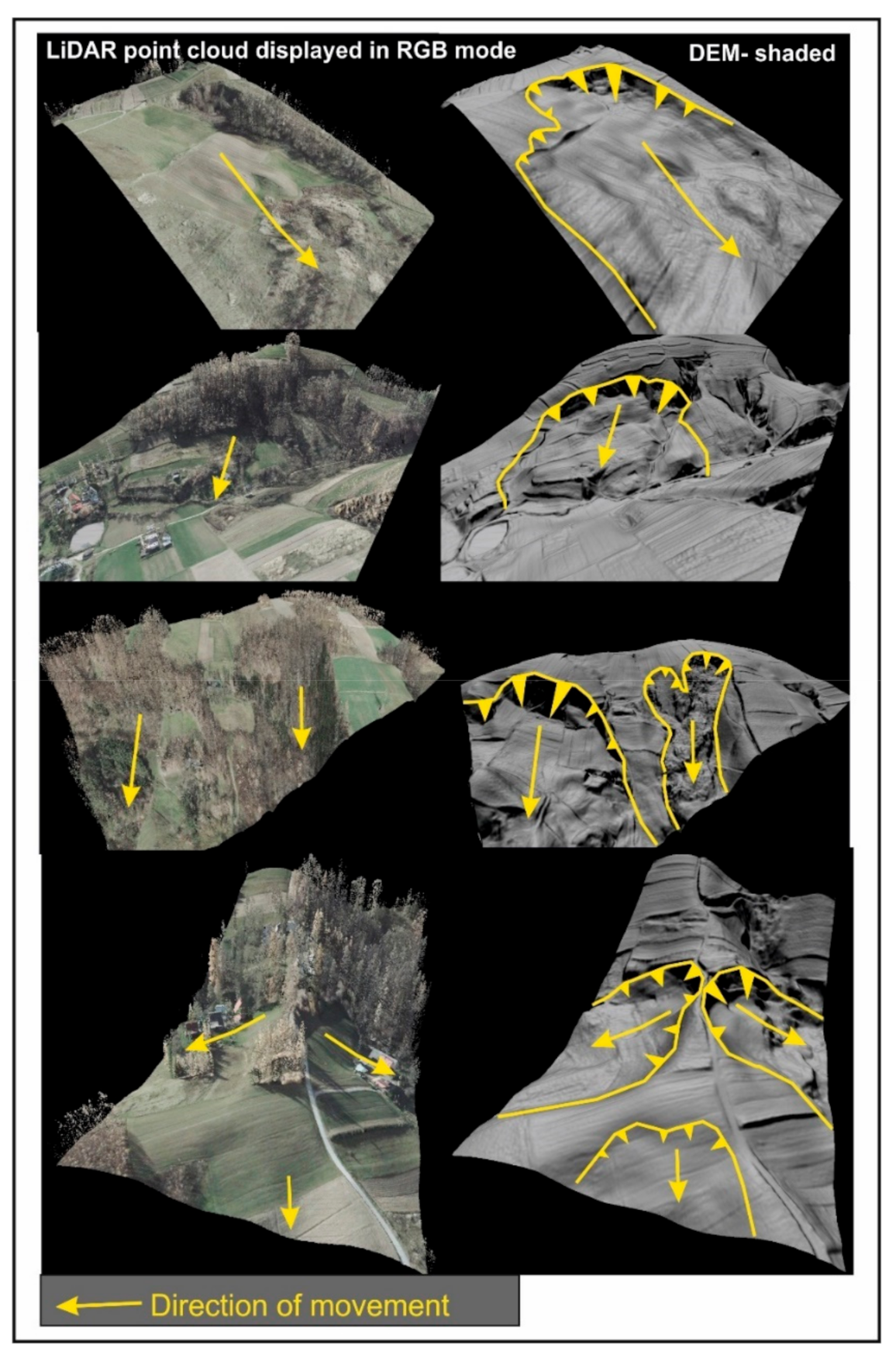
3.2. Airborne Laser Scanning (ALS)—LiDAR Data
3.3. Gaussian Low-Pass Filter
3.4. Weights-of-Evidence Method
4. Results
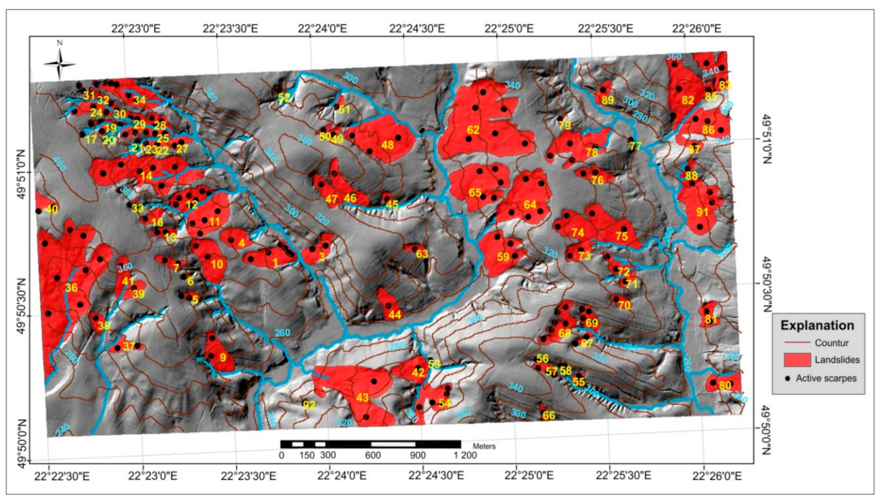
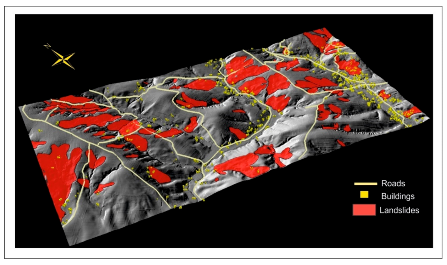
4.1. Landslide Inventory
4.2. Landslide Conditioning Factors and Their Analysis
4.3. Comparison of the Elevation Differences between the Digital Elevation Models (ALS and LPIS)
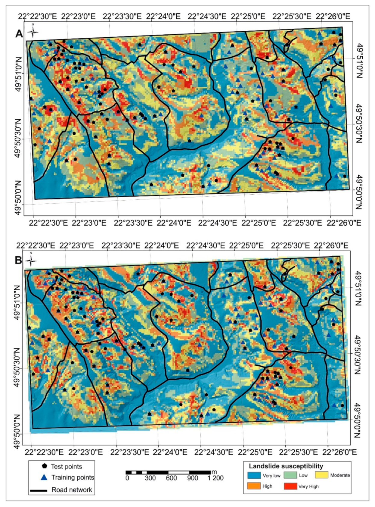
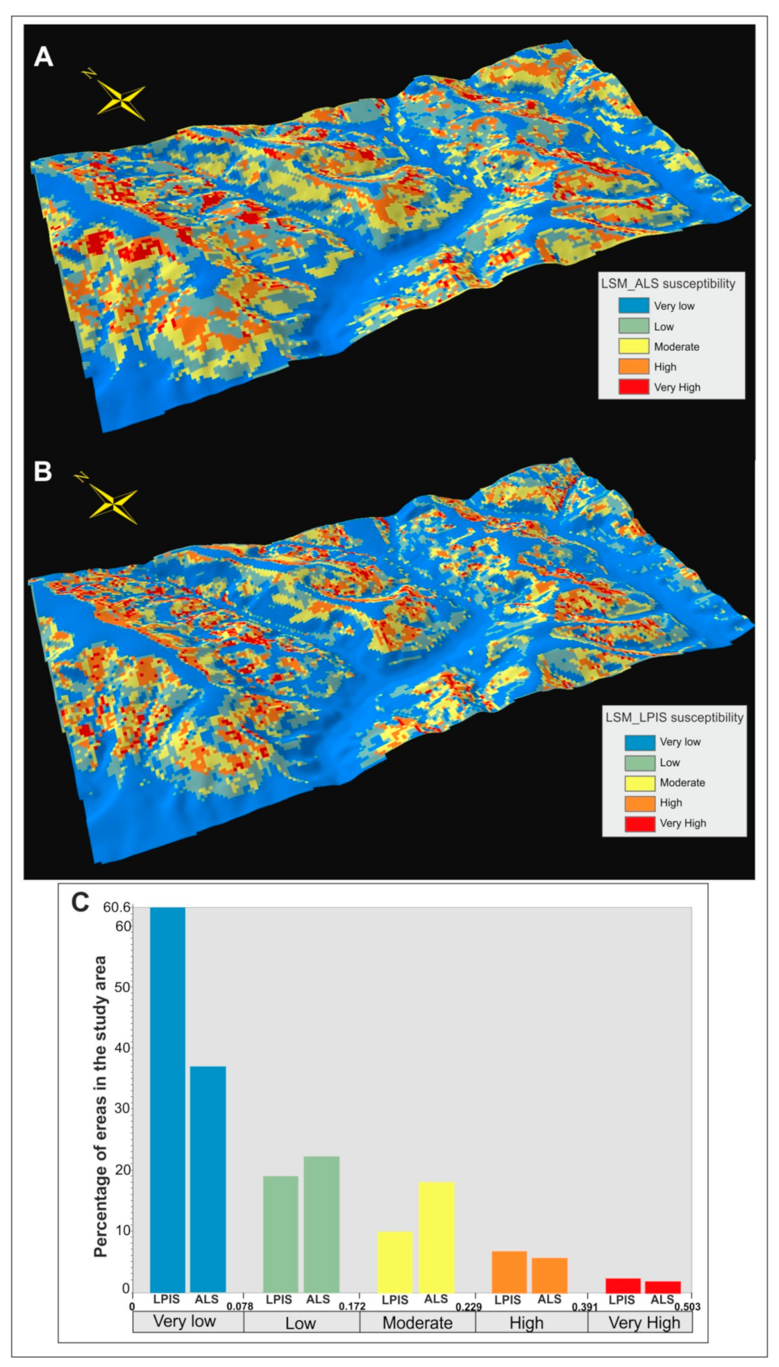
4.4. Landslide Susceptibility Maps
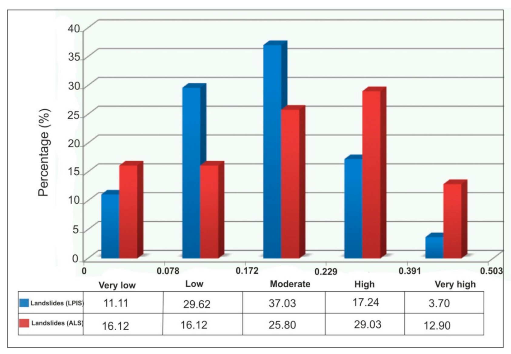
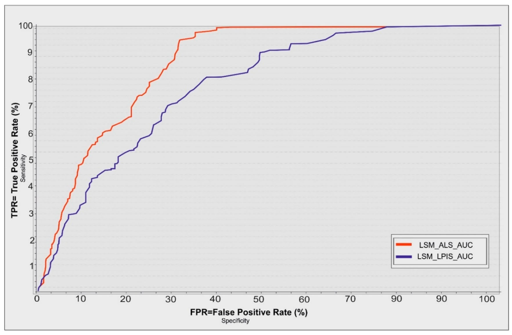
5. Validation
6. Discussion
7. Conclusions
Funding
Conflicts of Interest
References
- Aleotti, P.; Chowdhury, R. Landslide hazard assessment: Summary review and new perspectives. Bull. Eng. Geol. Environ. 1999, 58, 21–44. [Google Scholar] [CrossRef]
- Rączkowski, W.; Mrozek, T. Activating of landsliding in the Polish Flysch Carpathians by the end of the 20th century. Studia Geomorphol. Carpatho Balc. 2002, 36, 91–111. [Google Scholar]
- Bober, L. Landslide areas in the Polish part of the Carpathians flysh and their relationship with geological structure. Biult. Inst. Geolog. 1984, 340, 115–162. [Google Scholar]
- Kamiński, M. Landslide GIS analysis for selected area of the Dynów foreland. Arch. Photogramm. Cartogr. Remote Sens. 2006, 16, 279–287. [Google Scholar]
- Derron, M.H.; Jaboyedoff, M. LIDAR and DEM technique for landslides monitoring and characterization. Nat. Hazard Earth Syst. Sci. 2010, 10, 1877–1879. [Google Scholar] [CrossRef]
- Greve, C. Digital Photogrammetry an Addendum to the Manual of Photogrammetry. In American Society for Photogrammetry and Remote Sensing; Asprs Publications: Bethesda, MD, USA, 1996; pp. 121–123. [Google Scholar]
- Genelli, G.; Giusti, E.; Pizzaferri, G. Photogrammetric Technique for the Investigation of the Corniglio Landslide. In Applied Geomorphology, Theory and Practice; John Wiley & Sons: Hoboken, NJ, USA, 2002; pp. 23–28. [Google Scholar]
- Mora, P.; Baldi, P.; Casula, G.; Fabris, M.; Ghirotti, M.; Mazzioni, E.; Pesci, A. Global positioning systems and digital photogrammetry for monitoring of mass movements: Application to the Ca’ di Malta landslide (northern Apennines, Italy). Eng. Geol. 2003, 68, 103–121. [Google Scholar] [CrossRef]
- Dewitte, O.; Jasselette, J.-C.; Cornet, Y.; Eeckhaut, M.V.; Collignon, A.; Poesen, J.; Demoulin, A. Tracking landslide displacements by multi-temporal DTMs: A combined aerial sterophotogrammetric and LiDAR approach in western Belgium. Eng. Geol. 2010, 99, 11–22. [Google Scholar] [CrossRef]
- Kamiński, M. Application od photogrammetric methods to assess the dynamics of mass movements selected exmaples from Poland. Arch. Photogramm. Cartogr. Remote Sens. 2012, 24, 11–122. [Google Scholar]
- Meen, R.S.; Nachappa, G.T. Impact of Spatial Resolution of Digital Elevation Model on Landslide Susceptibility Mapping: A case Study in Kullu Valley, Himalayas. Geosciences 2019, 9, 67–74. [Google Scholar]
- Mohd, W.M.; Abdullah, M.A.; Hashim, S. Evaluation of Vertical Accuracy of Digital Elevation Models Generated from Different Sources: Case Study of Ampang and Hulu Langat, Malaysia. FIG Congress XXV.1-17. Geosciencies 2014, 9, 2–18. [Google Scholar]
- Miner, A.S.; Flentje, P.; Mazengarb, C.; Windle, D.J. Landslide Recognition using LiDAR derived Digital Elevation Models-Lessons learnt from selected Australian examples. In Proceedings of the Geologically Active Proceedings 11th IAEG Congregalia, Auckland, New Zealand, 5–10 September 2010; Volume 2, p. 352. [Google Scholar]
- Wang, B.; Shi, W.; Liu, E. Robust methods for assessing the accuracy of linear interpolated DEM. Int. J. Appl. Earth Obs. Geoinf. 2015, 34, 198–206. [Google Scholar] [CrossRef]
- Wu, B.; Tang, S.; Zhu, Q.; Tong, K.; Hu, H.; Li, G. Geometric integration of high-resolution satellite imagery and airborne LiDAR data for improved geopositioning accuracy in metropolitan areas. ISPRS J. Photogramm. Remote Sens. 2015, 109, 139–151. [Google Scholar] [CrossRef]
- Chang, K.T.; Doub, J.; Changc, Y.; Kuoa, C.P.; Xua, K.M.; Liud, J.K. Spatial resolution effects of digital terrain models on landslide susceptibility analysis. Int. Arch. Photogramm. Remote Sens. Spat. Inf. Sci. 2016, XLI-B8, 45–49. [Google Scholar]
- Komac, M. A landslide susceptibility model using the analytical hierarchy process method and multivariate statistics in perialpine Slovenia. Geomorphology 2006, 74, 17–28. [Google Scholar] [CrossRef]
- Wang, Q.; Guo, Y.; Li, W.; He, J.; Wu, Z. Predictive modeling of landslide hazards in Wen County, northwestern China based on information value, weights-of-evidence, and certainty factor. Geomat. Nat. Hazards Risk 2019, 10, 820–835. [Google Scholar] [CrossRef] [Green Version]
- Schlögel, R.; Marchesini, I.; Alvioli, M.; Reichenbach, P.; Rossi, M.; Malet, J.P. Optimizing landslide susceptibility zonation: Effects of DEM spatial resolution and slope unit delineation on logistic regression models. Geomorphology 2018, 301, 10–20. [Google Scholar] [CrossRef]
- Desmet, P.J.J. Effects of interpolation errors on the analysis of DEMs. Earth Surf. Process. Landf. 1997, 22, 563–580. [Google Scholar] [CrossRef]
- Florinsky, I.V. Accuracy of local topographic variables derived from digital elevation models. Int. J. Geogr. Inf. Sci. 1998, 12, 47–61. [Google Scholar] [CrossRef]
- Chaplot, V.; Darboux, F.; Bourennane, H.; Leguédois, S.; Silvera, N.; Phachomphon, K. Accuracy of interpolation techniques for the derivation of digital elevation models in relation to landform types and data density. Geomorphology 2006, 77, 126–141. [Google Scholar] [CrossRef]
- Fisher, P.F.; Tate, N.J. Causes and consequences of error in digital elevation models. Prog. Phys. Geogr. 2006, 30, 467–489. [Google Scholar] [CrossRef]
- Wise, S.M. The effect of GIS interpolation errors on the use of DEMs in geomorphology. In Landform Monitoring, Modeling and Analysis; Lane, S.N., Richards, K.S., Chandler, J.H., Eds.; Wiley: Chichester, UK, 1998; pp. 139–164. [Google Scholar]
- Thomas, J.; Prasannakumar, V.; Vineetha, P. Suitability of space-borne digital elevation models of different scales in topographic analysis: An example from Kerala, India. Environ. Earth Sci. 2015, 73, 1245–1263. [Google Scholar] [CrossRef]
- Zhang, W.; Montgomery, D. Digital elevation model grid size, landscape representation, and hydrologic simulations. Water Resour. Res. 1994, 30, 1019–1028. [Google Scholar] [CrossRef]
- Li, Z.L. A comparative study of the accuracy of digital terrain models (DTMs) based on various data models. ISPRS J. Photogramm. Remote Sens. 1994, 49, 2–11. [Google Scholar] [CrossRef]
- Bolstad, P.V.; Stowe, T. An evaluation of DEM accuracy: Elevation, slope, and aspect. Photogramm. Eng. Remote Sens. 1994, 60, 1327–1332. [Google Scholar]
- Edson, C.; Wing, M.G. LiDAR Elevation and DEM Errors in Forested Settings. Mod. Appl. Sci. 2015, 9, 139–157. [Google Scholar] [CrossRef] [Green Version]
- Bonham-Carter, G.F.; Agtberg, F.P.; Wright, D.F. Weight of evidence modeling: A new approach to mapping mineral potential. Statistical Applications in the Earth Sciences. In Geological Survey of Canada; Agterberg, F.P., Bonham-Carter, G.F., Eds.; Paper; F.A. Acland: Ottawa, ON, Canada, 1989; Volume 89, pp. 171–183. [Google Scholar]
- Bonham-Carter, G. Geographic Information System for Geoscientists: Modeling with GIS. In Computer Methods in the Geoscience; Pergamon Press: Oxford, UK, 1994; Volume 13, pp. 398–399. [Google Scholar]
- Agterberg, F.P.; Cheng, Q. Conditional independence test for weights of evidence modeling. Nat. Resour. Res. 2002, 11, 249–255. [Google Scholar] [CrossRef]
- Lee, S.; Choi, J.; Min, K. Landslide susceptibility analysis and verification using the Bayesian probability model. Environ. Geol. 2002, 43, 120–131. [Google Scholar] [CrossRef]
- Chung, J.O.F.; Fabbri, A.G. Validation of spatial prediction models for landslide hazard mapping. Nat. Hazard 2003, 30, 451–472. [Google Scholar] [CrossRef]
- Mrozek, T.; Poli, S.; Sterlascchini, S.; Zabuski, L. Landslide susceptibility assessment. A case study from the Beskid Niski Mts., Carpathains, Poland. In Proceedings of the Conference “Risks Caused by the Geodynamic Phenomena in Europe“, Wysowa, Poland, 20–22 May 2004; Volume 15, pp. 10–16. [Google Scholar]
- Neuhauser, B.; Terhorst, B. Landslide susceptibility assessment using ‘‘weights-of-evidence’’ applied to a study area at the Jurassic escarpment (SW-Germany). Geomorphology 2007, 86, 12–24. [Google Scholar] [CrossRef]
- Armas, I. Weights of Evidence method for landslide susceptibility mapping. Prahova Subcarpathians, Romania. Nat. Hazards 2011, 6, 31–38. [Google Scholar] [CrossRef]
- Kamiński, M. Application of LiDAR date to assess tha landslide susceptibility map using Weights of Evidence method—An example from Podhale region (Southern Poland). In Proceedings of the International Society for Photogrammetry and Remote Sensing ISPRS Congress, Prague, Czech Republic, 12–19 July 2016; Volume XLI-B1, pp. 25–29. [Google Scholar]
- Dai, F.C.; Lee, C.F.; Ngai, Y.Y. Landslide risk assessment and management: An overview. Eng. Geol. 2002, 64, 65–87. [Google Scholar] [CrossRef]
- Lee, S.; Choi, J.; Min, K. Probabilistic landslide hazard mapping using GIS and remote sensing data at Boun, Korea. Int. J. Remote Sens. 2004, 25, 2037–2052. [Google Scholar] [CrossRef]
- Nguyen, Q.P.; Bui, H.B. Landslide hazard mapping using Bayesian approach in GIS: Case study in YangSan area, Korea. In Proceedings of the International Symposium on GeoInformatics for Spatial-Infrastructure Development in Earth and Allied Sciences (GIS-IDEAS), Hanoi, Vietnam, 16–18 September 2004; Available online: http://gisws.media.osaka-cu.ac.jp/gisideas04/viewpaper.php?id=2 (accessed on 2 December 2020).
- Kamiński, M. Landslide susceptibility map in regionak scale an example from of San Valley in the Dynów Foothill. Biul. Państw. Inst. Geol. 2012, 452, 109–118. [Google Scholar]
- Ilia, I.; Tsangaratos, P. Applying weight of evidence method and sensitivity analysis to produce a landslide susceptibility map. Landslides 2016, 13, 379–397. [Google Scholar] [CrossRef]
- Varnes, D.J. Landslide hazard zonation: A review of principles and practice of the United Nations Educational, Scientific and Cultural Organization. Nat. Hazards 1984, 3, 127–138. [Google Scholar]
- Carrara, A.; Cardinali, M.; Detti, R.; Guzzetti, F.; Pasqui, V.; Reichenbach, P. GIS techniques and statistical models in evaluating landslide hazard. Earth Surf. Proc. Land 1991, 16, 427–445. [Google Scholar] [CrossRef]
- Van Westen, C.J. Application of Geographic Information Systems to Landslide Hazard Zonation. Ph.D. Thesis, Technical University Delft, Enschede, The Netherlands, 1993. [Google Scholar]
- Van Westen, C.J. Statistical Landslide Hazard Analysis, ILWIS 2.1 for Windows Application Guide; ITC Publication: Enschede, The Netherlands, 1997; pp. 73–84. [Google Scholar]
- Remondo, J.; Gonzales, A.; De Teran, J.R.D.; Fabrii, A.; Chung, C.J. Validation of landslide susceptibility maps; examples and applications from a case study in northern Spain. Nat. Hazards 2003, 1, 1–13. [Google Scholar] [CrossRef]
- Chung, C.J.; Fabbri, A.G. Probabilistic prediction models for landslide hazard mapping. Photogramm. Eng. Remote Sens. 1999, 65, 1389–1399. [Google Scholar]
- Glade, T. Vulenrability assessmnet in landslide risk analysis. Die Erde 2003, 134, 123–146. [Google Scholar]
- Glade, T.; Anderson, M.G.; Crozier, M.J. (Eds.) Landslide Hazard and Risk; Wiley: Chichester, UK, 2005; pp. 125–134. [Google Scholar]
- Van Westen, C.; Rengers, N.; Soeters, R. Use of geomorphological information in indirect landslide susceptibility assessment. Nat. Hazards 2003, 30, 399–419. [Google Scholar] [CrossRef]
- Van Westen, C.J.; Van Asch, T.W.J.; Soeters, R. Landslide hazard and risk zonation: Why is it still so difficult. Bull Eng. Geol. Environ. 2006, 65, 167–184. [Google Scholar] [CrossRef]
- Guzzetti, F. Landslide Hazard and Risk Assessment. Ph.D. Thesis, Rheinische Friedrich-Wilhelm-Universitaet Bonn, Bonn, Germany, 2006. Available online: http://hss.ulb.uni-bonn.de/dissonline/mathnatfak/2006/guzzettifausto/index.htm (accessed on 15 June 2009).
- Kamiński, M. Landslide susceptibility map: A case study from the Jodłówka region (Dynów Foothill)). Geol. Rev. 2007, 55, 779–784. [Google Scholar]
- Kouli, M.; Loupasakis, C.; Soupios, P.; Vallianatos, F. Landslide hazard zonation in high risk areas of Rethymno Prefecture, Crete Island, Greece. Nat. Hazards 2010, 52, 599–621. [Google Scholar] [CrossRef]
- Swets, J.A. ROC analysis applied to the evaluation of medical imaging techniques. Invest. Radiol. 1979, 14, 109–112. [Google Scholar] [CrossRef] [PubMed]
- Hanley, J.A. Receiver operating characteristic (ROC) methodology: The state of the art. Crit Rev. Diagn. Imaging 1989, 243. [Google Scholar]
- Kamiński, M.; Piotrowska, K. Detailed Geolgical Map of Poland at the Scale of 1:50,000 Kańczuga Sheet with Explanations. 2014. Available online: http:/bazadata.pgi.gov.pl/data/smgp/arkusze_skany/smgp 1006.jpg (accessed on 14 April 2014).
- Bartier, M.P.; Keller, P.C. Multivariate interpolation to incorporate thematic surface data using inverse distanece weighting. Comput. Geosci. 1996, 22, 795–799. [Google Scholar] [CrossRef]
- Jaboyedoff, M.; Oppikofer, T.; Abellán, A.; Derron, M.H.; Loye, A.; Metzger, R.; Pedrazzini, A. Use of LIDAR in landslide investigations: A review. Nat. Hazards 2012, 61, 5–28. [Google Scholar] [CrossRef] [Green Version]
- Milledge, G.D.; Stuart, L.; Warburton, J. Digital filtering of generic topographic data in geomorphological research. Earth Surf. Process. Landf. 2009, 34, 63–74. [Google Scholar] [CrossRef]
- Good, I.J. Statistical Evidence. In Encyclopedia of Statistics; Kotz, S., Johnson, N.L., Eds.; Wiley: New York, NY, USA, 1988; Volume 8, pp. 651–655. [Google Scholar]
- Bonham-Carter, G.F.; Agtberg, F.P.; Wright, D.F. Integration of geological datasets for gold exploration in Nova Scotia. Photogramm. Eng. Remote Sens. 1988, 54, 1585–1592. [Google Scholar]
- Agterberg, F.P.; Bonham-Carter, G.F.; Wright, D.F. Statistical Pattern Integration for Mineral Exploration. In Computer Applications in Resource Estimation Prediction and Assessment for Metals and Petroleum; Gaal, G., Merriam, D.F., Eds.; Pergamon Press: Oxford, UK, 1990. [Google Scholar]
- Weed, D.L. Weight of evidence: A review of concept and methods. Risk Anal. 2005, 25, 1545–1557. [Google Scholar] [CrossRef]
- Fan, D.; Cui, X.; Yuan, D.; Wang, J.; Yang, J.; Wang, S. Weight of Evidence Method and Its Applications and Development. Procedia Environ. Sci. 2011, 11, 1412–1418. [Google Scholar] [CrossRef] [Green Version]
- Dahal, R.K.; Hasegawa, S.; Nonomura, A.; Yamanaka, M.; Masuda, T.; Nishino, K. GIS-Based Weights-of-Evidence Modelling of Rainfall-Induced Landslides in Small Catchments for Landslide Susceptibility Mapping. Environ. Geol. 2008, 54, 311–324. [Google Scholar] [CrossRef]
- Schulz, W.H. Landslides Mapped Using LIDAR Imagery, Seattle, Washington. US Geol. Surv. Open File Rep. 2004, 11, 1–13. [Google Scholar]
- Ardizzone, F.; Cardinali, M.; Galli, M.; Guzzetti, F.; Reichenbach, P. Identification and mapping of recent rainfall-induced landslides using elevation data collected by airborne LiDAR. Nat. Hazards Earth Syst. Sci. 2007, 7, 637–650. [Google Scholar] [CrossRef] [Green Version]
- Bell, R.; Petschko, H.; Röhrs, M.; Dix, A. Assessment of landslide age, landslide persistence and human impact using airborne laser scanning digital terrain models. Geogr. Ann. 2012, 94, 135–156. [Google Scholar] [CrossRef]
- Kemp, L.D.; Bonham-Carter, G.F.; Raines, G.L. Arc-WofE: ArcView Extension for Weights of Evidence Mapping. Ottawa, ON, Canada, 1999. Available online: http://ntserv.gis.nrcan.gc.ca/sdm/ (accessed on 25 February 2002).
- Fabeis, M.; Pesci, A. Automated extraction in digital aerial photogrammetry: Precisions and validation for mass movement monitoring. Ann. Geophys. 2005, 48, 973–988. [Google Scholar]
- Stephen, E.; Reutebuch, R.; McGaughey, J.; Hans-Erik, A.; Ward, W.C. Accuracy of a high-resolution lidar terrain model under a conifer forest canopy. Can. J. Remote Sens. 2003, 29, 527–535. [Google Scholar] [CrossRef]
- Cama, M.; Conoscenti, C.; Lombardo, L.; Rotigliano, E. Exploring relationships between grid cell size and accuracy for debris-flow susceptibility models: A test in the Giampilieri catchment Sicily, Italy. Environ. Earth Sci. 2016, 753, 238–254. [Google Scholar] [CrossRef]
- Chang, K.T.; Merghali, A.; Yunus, A.P.; Pham, B.T.; Dou, J. Evaluating scale effects of topographic variables in landslide susceptibility models using GIS-based machine learning techniques. Sci. Rep. 2019, 9, 142–157. [Google Scholar] [CrossRef] [Green Version]
- Arnone, E.; Francipane, A.; Scarbaci, A.; Puglisi, C.; Noto, L.V. Effect of raster resolution and polygon-conversion algorithm on landslide susceptibility mapping. Environ. Model Softw. 2016, 84, 467–481. [Google Scholar] [CrossRef]
- Achour, Y.; Pourghasemi, H.R. How do machine learning techniques help in increasing accuracy of landslide susceptibility maps? Geosci. Front. 2019. [Google Scholar] [CrossRef]
- Barbieri, G.; Cambuli, P. The weight of evidence statistical method in landslide susceptibility mapping of the Rio Pardu Valley (Sardinia, Italy). In Proceedings of the 18th World IMACS/MODSIM Congress, Cairns, Australia, 13–17 July 2009; pp. 13–17. [Google Scholar]
- Neuhauser, B.; Damm, B.; Terhorst, B. GIS-based assessment of landslide susceptibility on the base of the Weights-of Evidence model. Landslides 2012, 9, 511–528. [Google Scholar] [CrossRef]


| RMS x (m) | RMS y (m) | RMS Total (m) | The Number of Aerial Images | Year |
|---|---|---|---|---|
| 0.44 | 0.36 | 0.32 | 12 | 2009 |
| Class | Area (km2) | Points | W+ | s (W+) | W− | s (W−) | C | s (C) | Stud (C) |
|---|---|---|---|---|---|---|---|---|---|
| Distance to fault (m) | |||||||||
| 0–50 | 6266 | 2 | −0.2108 | 0.7098 | 0.0049 | 0.1025 | −0.2157 | 0.7171 | −0.3008 |
| 50–100 | 6760 | 1 | −1.1767 | 1.0014 | 0.0234 | 0.1020 | −1.2001 | 1.0066 | −1.1922 |
| 100–150 | 7187 | 2 | 0.2091 | 0.7111 | −0.0039 | 0.1025 | 0.2130 | 0.7185 | 0.2964 |
| 150–200 | 7418 | 0 | |||||||
| >200 | 7578 | 3 | 0.6111 | 0.5823 | −0.0143 | 0.1031 | 0.6254 | 0.5913 | 1.0577 |
| Elevation (m.a.l.s) | |||||||||
| 230–235 | 1184 | 1 | −2.3963 | 1.0004 | 0.1086 | 0.1021 | −2.5048 | 1.0056 | −2.4909 |
| 235–255 | 2368 | 7 | −1.1414 | 0.3785 | 0.1790 | 0.1054 | −1.3204 | 0.3929 | −3.3605 |
| 255–312 | 3552 | 12 | −1.0074 | 0.2892 | 0.2778 | 0.1085 | −1.2853 | 0.3088 | −4.1615 |
| 312–363 | 4736 | 28 | −0.4453 | 0.1895 | 0.2541 | 0.1202 | −0.6993 | 0.2245 | −3.1155 |
| 363–415 | 5920 | 46 | −0.1701 | 0.1480 | 0.1792 | 0.1394 | −0.3492 | 0.2034 | −1.7176 |
| Aspect | |||||||||
| N | 1154 | 14 | 0.2537 | 0.2689 | −0.0367 | 0.1096 | 0.2904 | 0.2904 | 1.0001 |
| N–E | 2308 | 28 | 0.2539 | 0.1901 | −0.0859 | 0.1200 | 0.3398 | 0.2249 | 1.5111 |
| S–E | 3461 | 42 | 0.2540 | 0.1552 | −0.1555 | 0.1342 | 0.4094 | 0.2052 | 1.9953 |
| S–W | 4615 | 50 | 0.1393 | 0.1422 | −0.1271 | 0.1449 | 0.2664 | 0.2030 | 1.3121 |
| N–W | 5768 | 65 | 0.1790 | 0.1247 | −0.2798 | 0.1747 | 0.4588 | 0.2147 | 2.1374 |
| Slope (degrees) | |||||||||
| 0–2 | 822 | 0 | |||||||
| 2–5 | 2126 | 6 | −1.2140 | 0.4088 | 0.1677 | 0.1048 | −1.3816 | 0.4221 | −3.2735 |
| 5–13 | 3768 | 18 | −0.6856 | 0.2363 | 0.2505 | 0.1125 | −0.9361 | 0.2617 | −3.5773 |
| 13–20 | 5492 | 46 | −0.1205 | 0.1481 | 0.1203 | 0.1394 | −0.2408 | 0.2034 | −1.1841 |
| 20–54 | 7107 | 68 | 0.0138 | 0.1219 | −0.0305 | 0.1834 | 0.0443 | 0.2202 | 0.2012 |
| Topographic Ruggedness Index | |||||||||
| (−160)–(−2) | 1152 | 3 | −1.2960 | 0.5781 | 0.0876 | 0.1031 | −1.3836 | 0.5872 | −2.3561 |
| (−2)–(−1) | 2305 | 5 | −1.4788 | 0.4477 | 0.2010 | 0.1043 | −1.6798 | 0.4597 | −3.6543 |
| (−1)–0 | 3457 | 14 | −0.8527 | 0.2678 | 0.2540 | 0.1098 | −1.1068 | 0.2894 | −3.8240 |
| 0–1 | 4610 | 28 | −0.4452 | 0.1896 | 0.2540 | 0.1203 | −0.6993 | 0.2245 | −3.1150 |
| 1–12 | 5762 | 50 | −0.0859 | 0.1420 | 0.0981 | 0.1451 | −0.1841 | 0.2030 | −0.9066 |
| Distance to streams (m) | |||||||||
| 0–55 | 684 | 1 | −1.8469 | 1.0007 | 0.0566 | 0.1020 | −1.9036 | 1.0059 | −1.8924 |
| 55–69 | 912 | 10 | 0.1780 | 0.3180 | −0.0184 | 0.1071 | 0.1963 | 0.3355 | 0.5851 |
| 69–90 | 356 | 5 | 0.4293 | 0.4504 | −0.0186 | 0.1042 | 0.4479 | 0.4623 | 0.9690 |
| 90–120 | 491 | 7 | 0.4430 | 0.3807 | −0.0272 | 0.1053 | 0.4701 | 0.3950 | 1.1902 |
| Class | Area (km2) | Points | W+ | s (W+) | W− | s (W−) | C | s (C) | stud (C) |
|---|---|---|---|---|---|---|---|---|---|
| Distance to fault (m) | |||||||||
| 0–50 | 6266 | 61 | −0.0023 | 0.1287 | 0.0093 | 0.2595 | −0.0116 | 0.2896 | −0.0399 |
| 50–100 | 6760 | 66 | 0.0006 | 0.1237 | −0.0039 | 0.3178 | 0.0045 | 0.3410 | 0.0131 |
| 100–150 | 7187 | 70 | −0.0019 | 0.1201 | 0.0221 | 0.4103 | −0.0240 | 0.4275 | −0.0561 |
| 150–200 | 7418 | 72 | −0.0054 | 0.1184 | 0.1025 | 0.5027 | −0.1079 | 0.5165 | −0.2089 |
| >200 | 7578 | 74 | 0.0008 | 0.1168 | −0.0283 | 0.7105 | 0.0291 | 0.7200 | 0.0404 |
| Elevation (m.a.l.s) | |||||||||
| 230–235 | 903 | 1 | −2.1775 | 1.0006 | 0.0841 | 0.1021 | −2.2616 | 1.0057 | −2.2487 |
| 235–255 | 2267 | 9 | −0.8978 | 0.3340 | 0.1591 | 0.1066 | −1.0568 | 0.3506 | −3.0144 |
| 255–312 | 3786 | 18 | −0.7168 | 0.2363 | 0.2689 | 0.1125 | −0.9857 | 0.2617 | −3.7667 |
| 312–363 | 5333 | 41 | −0.2331 | 0.1568 | 0.2093 | 0.1332 | −0.4425 | 0.2058 | −2.1504 |
| 363–415 | 6845 | 63 | −0.0517 | 0.1266 | 0.1003 | 0.1699 | −0.1520 | 0.2119 | −0.7173 |
| Aspect | |||||||||
| N | 837 | 7 | −0.1670 | 0.3796 | 0.0142 | 0.1059 | −0.1812 | 0.3941 | −0.4599 |
| N–E | 2236 | 29 | 0.2766 | 0.1869 | −0.0981 | 0.1218 | 0.3747 | 0.2231 | 1.6794 |
| S–E | 3412 | 43 | 0.2474 | 0.1535 | −0.1609 | 0.1367 | 0.4083 | 0.2055 | 1.9869 |
| S–W | 4578 | 53 | 0.1614 | 0.1382 | −0.1651 | 0.1514 | 0.3265 | 0.2050 | 1.5931 |
| N–W | 6019 | 66 | 0.1066 | 0.1238 | −0.1950 | 0.1803 | 0.3016 | 0.2187 | 1.3787 |
| Slope (degrees) | |||||||||
| 0–2 | 807 | 0 | |||||||
| 2–5 | 2062 | 7 | −1.0735 | 0.3786 | 0.1622 | 0.1060 | −1.2357 | 0.3932 | −3.1429 |
| 5–13 | 3681 | 18 | −0.7070 | 0.2363 | 0.2669 | 0.1132 | −0.9739 | 0.2620 | −3.7170 |
| 13–20 | 5311 | 44 | −0.1765 | 0.1514 | 0.1747 | 0.1382 | −0.3512 | 0.2050 | −1.7134 |
| 20–54 | 6804 | 70 | 0.0422 | 0.1201 | −0.1018 | 0.1933 | 0.1440 | 0.2276 | 0.6325 |
| Topographic Ruggedness Index (TRI) | |||||||||
| (−160)–(−2) | 782 | 2 | −1.2860 | 0.8780 | 0.0576 | 0.2031 | −1.6837 | 0.5630 | −2.1321 |
| (−2)–(−1) | 2078 | 10 | −0.7246 | 0.3170 | 0.1304 | 0.1078 | −0.8550 | 0.3348 | −2.5536 |
| (−1)–0 | 3734 | 20 | −0.6168 | 0.2242 | 0.2505 | 0.1147 | −0.8673 | 0.2518 | −3.4437 |
| 0–1 | 5332 | 44 | −0.1816 | 0.1514 | 0.1808 | 0.1382 | −0.3624 | 0.2050 | −1.7682 |
| 1–12 | 6778 | 67 | 0.0005 | 0.1228 | −0.0012 | 0.1835 | 0.0018 | 0.2208 | 0.0080 |
| Distance to streams (m) | |||||||||
| 0–55 | 684 | 1 | −1.8948 | 1.0007 | 0.0600 | 0.1021 | −1.9548 | 1.0059 | −1.9433 |
| 55–69 | 1582 | 8 | −0.6494 | 0.3545 | 0.0848 | 0.1060 | −0.7341 | 0.3700 | −1.9844 |
| 69–90 | 1931 | 12 | 0.4424 | 0.2896 | 0.0808 | 0.1084 | −0.5233 | 0.3092 | −1.6924 |
| 90–120 | 10168 | 98 | 0.0600 | 0.1021 | 0.8948 | 0.0007 | 1.9548 | 1.0059 | −1.9433 |
Publisher’s Note: MDPI stays neutral with regard to jurisdictional claims in published maps and institutional affiliations. |
© 2020 by the author. Licensee MDPI, Basel, Switzerland. This article is an open access article distributed under the terms and conditions of the Creative Commons Attribution (CC BY) license (http://creativecommons.org/licenses/by/4.0/).
Share and Cite
Kamiński, M. The Impact of Quality of Digital Elevation Models on the Result of Landslide Susceptibility Modeling Using the Method of Weights of Evidence. Geosciences 2020, 10, 488. https://0-doi-org.brum.beds.ac.uk/10.3390/geosciences10120488
Kamiński M. The Impact of Quality of Digital Elevation Models on the Result of Landslide Susceptibility Modeling Using the Method of Weights of Evidence. Geosciences. 2020; 10(12):488. https://0-doi-org.brum.beds.ac.uk/10.3390/geosciences10120488
Chicago/Turabian StyleKamiński, Mirosław. 2020. "The Impact of Quality of Digital Elevation Models on the Result of Landslide Susceptibility Modeling Using the Method of Weights of Evidence" Geosciences 10, no. 12: 488. https://0-doi-org.brum.beds.ac.uk/10.3390/geosciences10120488