Article

Revisiting the Paleo Elbe Valley: Reconstruction of the Holocene, Sedimentary Development on Basis of High-Resolution Grain Size Data and Shallow Seismics

by
Svenja Papenmeier
1,* and
H. Christian Hass
2,†
1
Leibniz Institute for Baltic Sea Research Warnemünde, 18119 Rostock, Germany
2
Alfred Wegener Institute, Helmholtz Centre for Polar and Marine Research, Wadden Sea Research Station, Hafenstraße 43, 25992 List, Germany
*
Author to whom correspondence should be addressed.
Decease.
Submission received: 3 November 2020 / Revised: 4 December 2020 / Accepted: 9 December 2020 / Published: 18 December 2020

Abstract

:
The Paleo Elbe Valley is the most prominent subsurface structure in the southern North Sea. During the Weichselian (marine isotope stage (MIS) 2), the valley traversed the exposed sea floor and drained the southern margin of the Scandinavian ice sheet. Today the valley is filled with up to 16 m thick sediments, but the responsible processes and drivers remain unknown. To unravel these processes and describe the valley’s evolution with Holocene transgression, we use shallow seismic data and vertical high-resolution grain-size core data. At the base of the western shore, supralittoral fine sands are overlain by a thin layer of clay dated to 9.8 cal. ka BP. The major sediment package consists of marine silt with internal seismic reflectors inclined in a northeastern direction, indicating a sediment transport from the southwest. The valley infill started when the western shore was flooded around 9.6 cal. ka BP and can be divided into two phases. During the first one (9.6–8.1 cal. ka BP) the sedimentation rate was highly driven by wind and waves. The second phase (8.1–5.0 cal. ka BP) was mainly tidal dominated but shows also storm event deposits in the north. Around 5.0 cal. ka BP the valley was almost filled.

Graphical Abstract

1. Introduction

The North Sea is a young shallow shelf sea shaped by several glacial advances and retreats during the Pleistocene [1]. Sedimented sequences of glaciofluvial or glacial deposits and complex tunnel valleys [2,3] result from the Elsterian (marine isotope stage (MIS) 12) and Saalian (MIS 6) glaciations covering the North Sea and northern Europe [4], including the Baltic region. The most prominent and largest morphological submerged feature is the Paleo Elbe Valley (PEV), also known as the Heligoland Channel [5,6]. During the Last Glacial Maximum, when sea level had the lowest standing at about 120 m below the present, the PEV traversed the exposed North Sea floor, draining the southern margin of the Scandinavian ice sheet in the direction of the Norwegian Channel (Figure 1).
The course and shape of the valley are known principally from a survey done by Figge [5], who investigated the thickness of the Holocene sediment layer in the German Bight with an analog sediment echo sounder geo-referenced with a DECCA navigation system, and was revised by [7,8,9]. The valley stretches from Heligoland towards the northwest, passing the Dogger Bank in the east [6], with a width of 25 km close to Heligoland and widening to 40 km in the north [5]. The bottom depths in the central part of the valley are 38 m southwest of Heligoland and 56 m close to the White Bank (slope = 0.01°). A Geest landscape extends east of the valley [5], characterized by reworked moraine deposits [10,11]. To the west of the valley the landscape is rather flat, similar to the present North Sea floor [5]. In the center of the valley some smaller elevations not larger than 2 m were interpreted as local sandbanks [5]. A connection to the present Elbe and Weser River remains unclear. Northwest of Heligoland (52 km) a tributary stream, possibly the Eider, comes from the east [5]. In the southeast, there is a complex system of Quaternary tunnel valleys [2], from which the most prominent structure is the submerged Paleo-Ems [12].
The dynamic paleogeography of the North Sea with the increasing Holocene sea level has widely been studied. The inundation of the North Sea started in the north with the early Holocene transgression [14]. With sea-level rise, the paleo valley transformed into a fjord-like estuary. Biostratigraphic records south of the Dogger Bank described a change from riverine to estuarine around 11 cal. ka BP [6]. Around 9.5 ka BP, the terrestrial connection between Britain and Europe began to be inundated [15]. With increasing sea level, the Dogger Bank became an island (~9 ka cal. BP). At 8.56 cal. ka BP, full marine conditions were described by Konradi [6] south of the Dogger Bank, and the connection between the English Channel and the southern North Sea opened at 8.3 cal. ka BP [16]. At ca 8.15 cal. ka BP, the Storrega tsunami had a catastrophic impact on the coastal environment, affecting the Mesolithic communities. However, the extent of the tsunami is still under debate. Notably, tsunami deposits correlating in timing with the Storrega event have recently been described in the southern North Sea at the head of a paleo-river system offshore of the Norfolk coast [17]. Around 7.5 cal. ka, the Dogger Bank was finally flooded [18] and the North Sea had almost the present shape [15].
The changes in the relative sea level (RSL) for the southern North Sea have been reconstructed by Behre [19], updated by Vink et al. [20], and debated by Baeteman et al. [21], amongst others. The reconstruction of the RSL is challenging especially for offshore areas because index points are mainly available for the coastal regions. Furthermore, isostatic movements dynamically changed from the southwest (Netherlands) to the northeast (Denmark), demanding more detailed local sea-level reconstructions.
The Holocene hydrographic situation has been modeled by several authors [22,23,24,25,26,27]. At the beginning of the Holocene, high bed shear stress induced by wind waves dominated suspended sediment transport [26]. With increasing sea level and related depth change, wave influence became gradually reduced and bed-load sediment transport by tidal currents became more important [25]. The opening of the English Channel increased the inward and outward water flow of the North Sea basin and hence strengthened the tidal regime. At around 6 cal. ka BP, the system showed a hydrographic situation analogous to the modern one [23].
The present seafloor surface shows only little evidence of the large paleo valley, which is almost completely filled [5]. Only small differences in height exist at the eastern shore at the transition to the former moraine landscape. The up to 16 m thick sediment infill is described as Holocene accumulation [5]. Comparable accumulations with up to 10 m exist only in the coastal zone [28]. In the remaining offshore area of the German Bight is the Holocene sediment layer, relatively thin and usually holding less than 5 m in the offshore areas [29].
A sedimentologically homogeneous sediment unit was previously suggested within the PEV because of missing impedance changes [5]. However, sedimentological characterization is still missing, and the timing, sediment sources, and environmental circumstances during the infill process of the valley remain unknown.
This study aims to shed new light on the development of the PEV within the German sector and contribute to the understanding of the past depositional environment that enabled the massive sediment infill of the valley. High vertical resolution grain-size data (1 cm) combined with an area-wide raster of shallow seismic data enable a comprehensive analysis of the historical process of sedimentary valley infill with the successive Holocene sea-level rise. Additional accelerated mass spectroscopy (AMS) 14C age determinations of selected samples support the linkage between sediment petrography, lithology, and seismic sequences to the RSL development known from literature.

2. Study Site

The study area is located in the German Bight of the southeastern North Sea, with water depths ranging from 25 to 50 m. East of the suggested PEV, in the vicinity of the Sylt Outer Reef Special Area of Conservation, the surface sediments consist of heterogeneously distributed coarse material partly covered by a thin layer (decimeter to meter) of Holocene marine sand [1,10,11,30,31,32]. Closer to the PEV, lag deposits prevail, containing a mixture of sand, gravel, pebbles, cobbles, and boulders. Eastwards, with increasing distance, the coarse sediments are characterized by poorly sorted gravel to very coarse sand without any boulders and blocks. The surface sediments of the central Paleo Elbe valley are dominated by fine to very fine sands [11], with mean grain size decreasing from the west (130 µm) to the east (80 µm).
The seafloor is under the permanent influence of near-bed currents, which are induced by semidiurnal tidal currents and by storm-induced waves originating mainly from the northwest. The latter can be up to 7 m in height and can reach the seafloor in the shallower parts of the study area. The residual current in the region of the PEV is from west to east and turns to the north at the eastern shore of the PEV [33,34,35]. The present sediment transport load is smaller than 55 m³/m/a [35].

3. Materials and Methods

3.1. Shallow Seismic Data

In an area of about 8300 km², 10,600 km of sub-bottom profiles were recorded during four cruises with the German research vessel RV Heincke (Figure 1, Table 1). Track lines of the first three campaigns are parallel, with track spacing of 400 m (HE00, HE415) and 1600 m (HE436), respectively. The high number of parallel lines is related to a surface sediment mapping campaign (project SedAWZ) with sidescan sonar, which was the main focus of these three campaigns. Profiles of cruise HE438 were acquired to specify coring locations. The vibro cores were taken during cruise HE439.
A narrow-beam parametric sediment echo sounder (pSES) SES-2000 medium (Innomar Technology GmbH, Rostock, Germany) was used to image the internal sediment structure. The nonlinear interference of two propagating and slightly different frequencies generates a secondary, low frequency with improved signal-to-noise ratio, which results in high vertical and lateral resolution [40,41]. The vertical resolution is between 5 and 25 cm depending on the used low (secondary) frequency and pulse length. The horizontal resolution is 30–40 cm at a survey speed of 5–6 knots and a ping rate of 7–10 pps. For more details, see Papenmeier and Hass [11].
The depth of distinct seismic reflectors was identified and exported with the software package Kingdom 2019 (IHS Markid Ltd.). The reflector of the valley base was selected in all data. Internal structures were only selected in the central and southern part of the valley where the data density was high. Tidal effects were reduced by normalizing the water depth with the bathymetric data provided by the German Federal Maritime and Hydrographic Agency. Point data were interpolated and gridded with Surfer 16 (Golden Software) using a moving average.

3.2. Coring and Grain-Size Analysis

Four sediment cores were taken on 6 March 2015 (Table 2, Figure 1) using a vibro corer manufactured by med consultants in Rostock, Germany. The sampling stations were chosen along a seismic transect where data showed the thinnest sediment layers, and hence a maximum temporal sequence was achievable.
After retrieval, the core liners were cut into 1 m pieces and stored at 4 °C. Back in the laboratory, the cores were opened and the sediment lithology was macroscopically described and photographed as part of the standard routines.
Samples for grain-size analysis (1–3 cm³) were taken with 1 cm resolution and stored in a 100 mL NUNC plastic container. Before the measurements, all samples underwent standard pre-treatment and removal of carbonate and organic matter, according to Hass et al. [42]. Grain-size measurements were performed on a CILAS 1180L (3P Instruments GmbH & Co. KG, Odelzhausen, Germany) laser-diffraction particle sizer (range: 0.04 to 2500 µm). Grain-size statistics are based on the volume of percentage data and the geometric (modified) Folk and Ward graphical method [43] using the program GRADISTAT (version 8.0) [44].

3.3. Age Determinations

A total of five calcareous shell fragment samples for accelerator mass spectrometry (AMS) 14C age determinations were hand-picked from the four silty to fine sand cores (Table 3). These were measured in the Beta Analytic Inc. facilities in Miami, Florida (USA). The calibration to calendar years was carried out using the MARINE13 database and a ∆R of 29 years [45].

4. Results

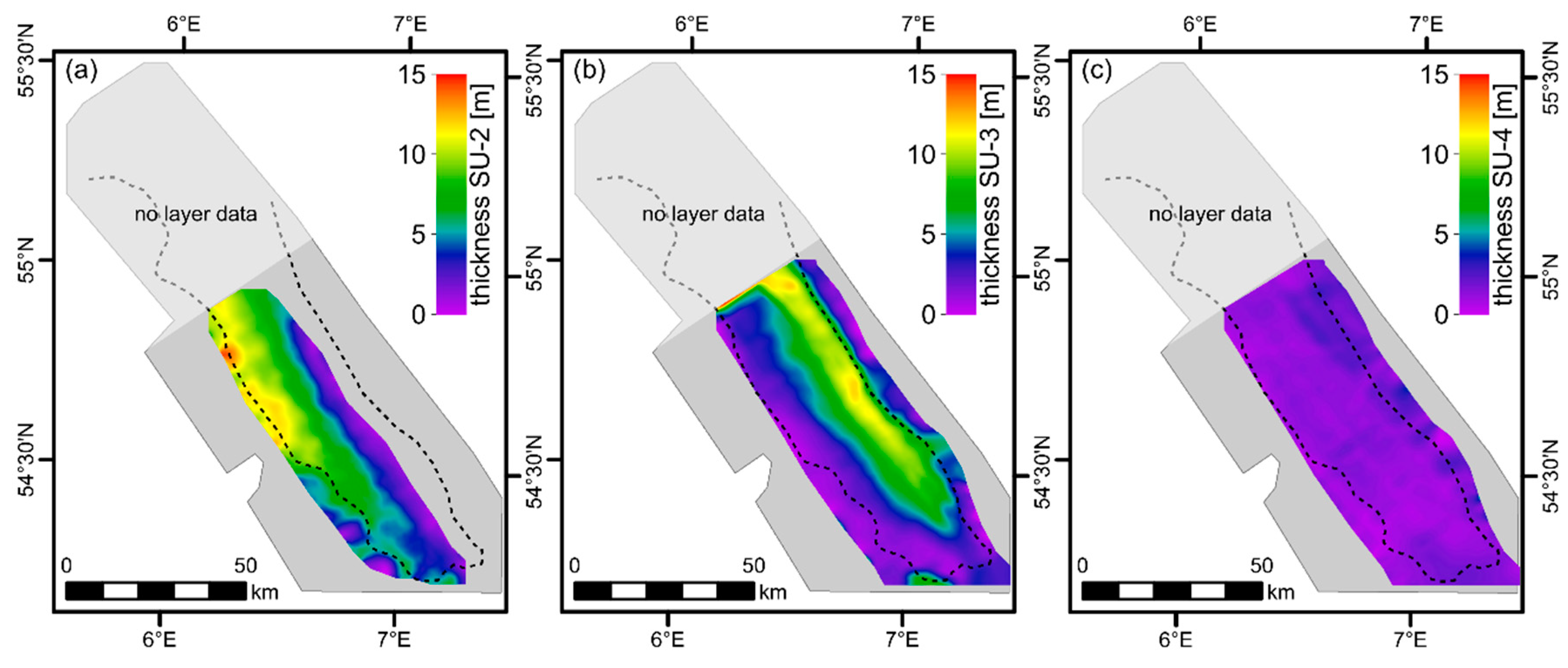
4.1. Seismic Facies Analysis

The base of the PEV was delineated by a strong seismic reflector (SR-A) at the eastern and western shores. In the central part of the valley, scattered incisions were noticeable and the reflector became less clear or was blank (Figure 2a–c,g and Figure 3a). The SR-A defined the upper boundary of the lowest identifiable seismic unit 1 (SU-1) (Figure 2d–f). The unit was characterized by chaotic and structureless reflection and energy rapidly dissipated.
The course of the PEV was almost straight from southeast to northwest (Figure 3). In the southern part, the valley had a width of 20 km and widened towards the northern outlet to more than 30 km width. The basin of the valley moved from 45 m in the south to 62 m below present sea level (b.p.s.l.) in the north, resulting in a gradient of 0.006° (Figure 3a,b). The valley basin was located approximately 10 m below the upper shoreline. The minimum depth of the shores was 32 m below mean sea level. The western shore was on average slightly steeper (0.075° ± 0.03°, max. 0.15°) than the eastern shore (0.06° ± 0.02°, max. 0.12°). The lower mean values at the eastern shore were related to several bays.
The valley was filled by a 10–15 m thick sediment package (Figure 2; Figure 3c). The final thickness was related to the morphology of the valley and the distribution of the accommodation space, with largest values in the central basin and with decreasing thickness towards the shorelines. The western shoreline was covered by sediments but the eastern shoreline was partly free of sediment cover.
On top of the structureless SU-1, the infill can be divided into three major seismic sequences (SU-2–4), as exemplarily shown by the three cross-sections in Figure 2:
Seismic unit 2 (SU-2): The lowest unit of the infill was defined by prograding, continuous, high-amplitude reflectors that had a vertical distance of some decimeters (maximum 1 m) (Figure 2a–c). The unit thickness was up to 14.3 m and decreased towards the eastern shore but increased downstream (Figure 4a). The unit’s upper boundary (SR-B) was parallel to the layered reflectors. The SR-B boundary was located at a depth between −38 m and −52 m b.p.s.l. and had a mean dip angle of 0.026° ± 0.011° (Figure 5a and Figure 6). In seismic profile 1, SU-2 showed a disconformity at the western shore (Figure 2a). In the central part of the valley the lower part of the unit was blank (Figure 2a).
Seismic unit 3 (SU-3): This unit had a maximum thickness of 14.4 m (Figure 4b). The highest thickness occurred along the eastern shore and increased downstream. The unit’s upper boundary (SR-G) was between -−48.9 m and −35.5 m b.p.s.l. and had a mean dip angle of 0.016° ± 0.01° (Figure 5b and Figure 6). In the south, the unit was free of internal reflections. Following the course of the valley, low-amplitude reflectors occurred and further divided the unit into up to six sub-units. In the central part of the valley, the subunits showed internal, parallel reflectors as described for SU-2.
Seismic unit 4 (SU-4): The uppermost sediment unit was present across the complete PEV and showed no distinct internal structure (Figure 2a–c). The unit was not thicker than 5.3 m (Figure 4c). The unit’s upper limit was given by the seafloor. The reflector defining the lower unit limit (SR-G) was strong at the western shore and decreased in amplitude towards the eastern shore.

4.2. Macroscopic Core Description

Detailed lithology descriptions and core photographs can be found in the database PANGAEA (Table 4). In general, the sediments of the four cores consisted of silty to fine sand of a dark grayish brown color, whereas the upper 3.5 m of core 1 (corresponding to SU-3 and SU-4) was a dark grayish-yellow.
Changes in grain size were generally gradual. The most prominent change was present in the lowest section of core 4 (Figure 7). The base of core 4 was dominated by a pale brownish fine sand, partly with organic remains. Above 4.6 m, the fine sand got darker and several clay-like to silty fine sand layers with sharp boundaries occurred up to a depth of 4.0 m.
In all cores, increased shell content was found at or close to the topmost layer. At coring stations 3 and 4, this shell layer was located at the sediment surface. At stations 1 and 2, shells were present at a depth of about 20–40 cm. In core 1, there were indications of increased bioturbation from the base up to 3.5 m core depth and in core 3 between 0.7 and 4 m.

4.3. Grain-Size Analysis

From the mean grain size measured in 1 cm intervals, a general constant upward coarsening was present in cores 1–3 and the middle section of core 4 (0.53–3.61 m; Figure 8). The mean grain size varied between coarse silt (40 µm) and fine sand (180 µm). The individual size classes show that the frequency of fine and medium sand increased upwards, whereas the frequency of very fine sand and silt decreased (Figure 8). In all cores, the clay content was generally less than 10%.
In core 4, abrupt changes in mean grain size occurred at 0.53 m core depth and in the lower section below 3.61 m. In the lower section the mean grain size was relatively high (130–215 µm). The main size classes were fine sand (~60%) and medium sand (up to 30%). This section was interrupted by three 1–2 cm-thick layers at 4.17, 4.56, and 4.58 m where clay and silt were dominant. The minimum mean grain size of these layers was 4 µm.
The sorting of the sediments was moderate to poor and decreased almost linearly with increasing mean grain size, except for the samples of SU-1 at coring station 4 (Figure 9). The samples of SU-1 had moderately well sorted sediments, independent of the mean grain size. Although SU-2 indicated the same linear relationship independent of the coring station, SU-3 and SU-4 showed a coring site-dependent relationship between sorting and mean grain size.
Most of the sediments were very leptokurtic and fine to very fine skewed, again with the exception of SU-1, which represented an endmember for all analyzed samples (Figure 10). The sediments from SU-1 were leptokurtic and varied from symmetric to fine skewed. For all units, the sediments’ grain size showed a negative, linear relationship between skewness and kurtosis, which changed to a positive, linear trend at a skewness value of around −0.5. Notably, these data (skewness < –0.5) represent the peaks of low mean grain sizes that punctuated the cores throughout (Figure 8).
The sediments’ sorting, skewness, and kurtosis did not show any significant trends over core depth. However, following the distinct seismic reflectors and the surface sediments geographically, regional differences from west to east were obvious in the grain size parameters (Figure 11). The individual values represent the mean of samples 5 cm above and below the reflector depth. Notably, there was a sediment fining towards the east, and the sorting decreased (from moderate to poor), except for the surface sediments. All sediments were very fine skewed and very leptokurtic. Again, minor changes occurred from west to east with the exception of the surface samples.

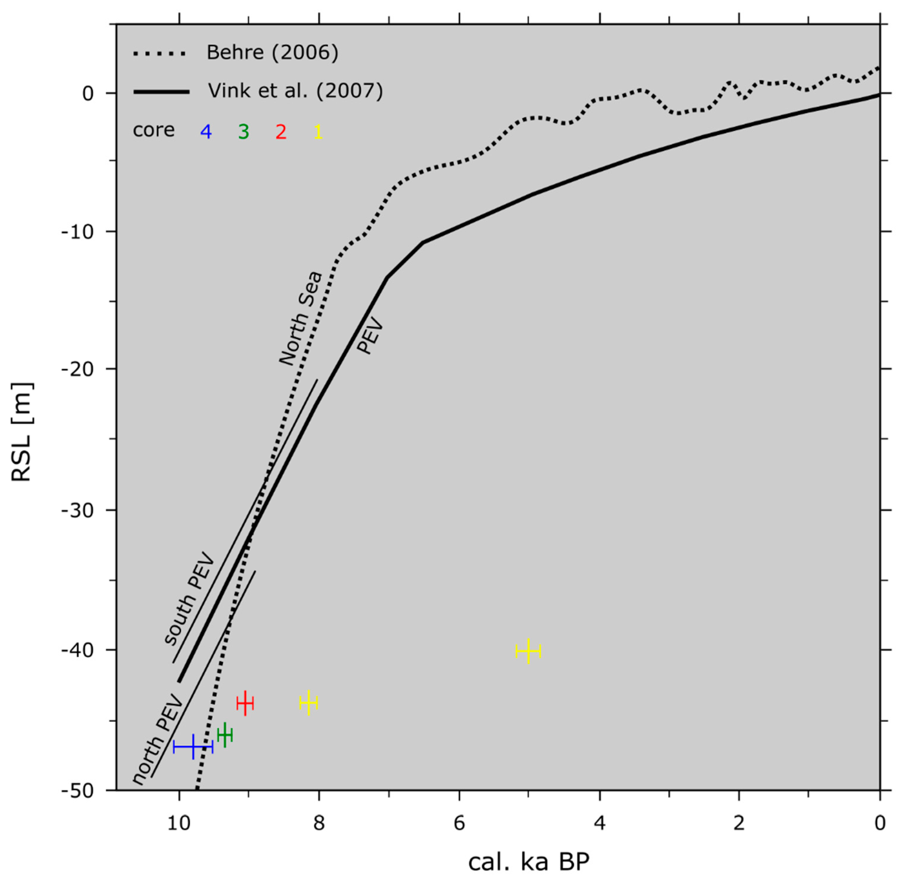
4.4. Age-Depth Model and Sedimentation Rates

The results of the AMS 14C age determinations are shown in Table 3 and are marked in the relative sea-level plot in Figure 12. Samples from cores 1–3 are clearly located below the RSL whereas the depositional environment of the sample from core 4 is uncertain. The sample was located above or below the RSL depending on the RSL curve considered.
The dated samples could be related to distinct seismic reflectors (Figure 2g). Consequently, the top of SU-1 (SR-A) was dated to ~9817 cal. yr BP. An age of ~8165 cal. yr BP was determined close to the top of SU-2 (SR-F), and an age of ~5027 cal. yr BP close to the top of SU-3 (SR-G).
The sedimentation rate calculated from the seismics varied between 0.3 and 1.8 m per century (Table 5). Generally, the sedimentation rate decreased from the western to eastern coring sites. The highest sedimentation was determined between 9.3 and 9.0 cal. ka BP, which led to a temporal decrease in water depth at the coring stations (Figure 13).

5. Discussion

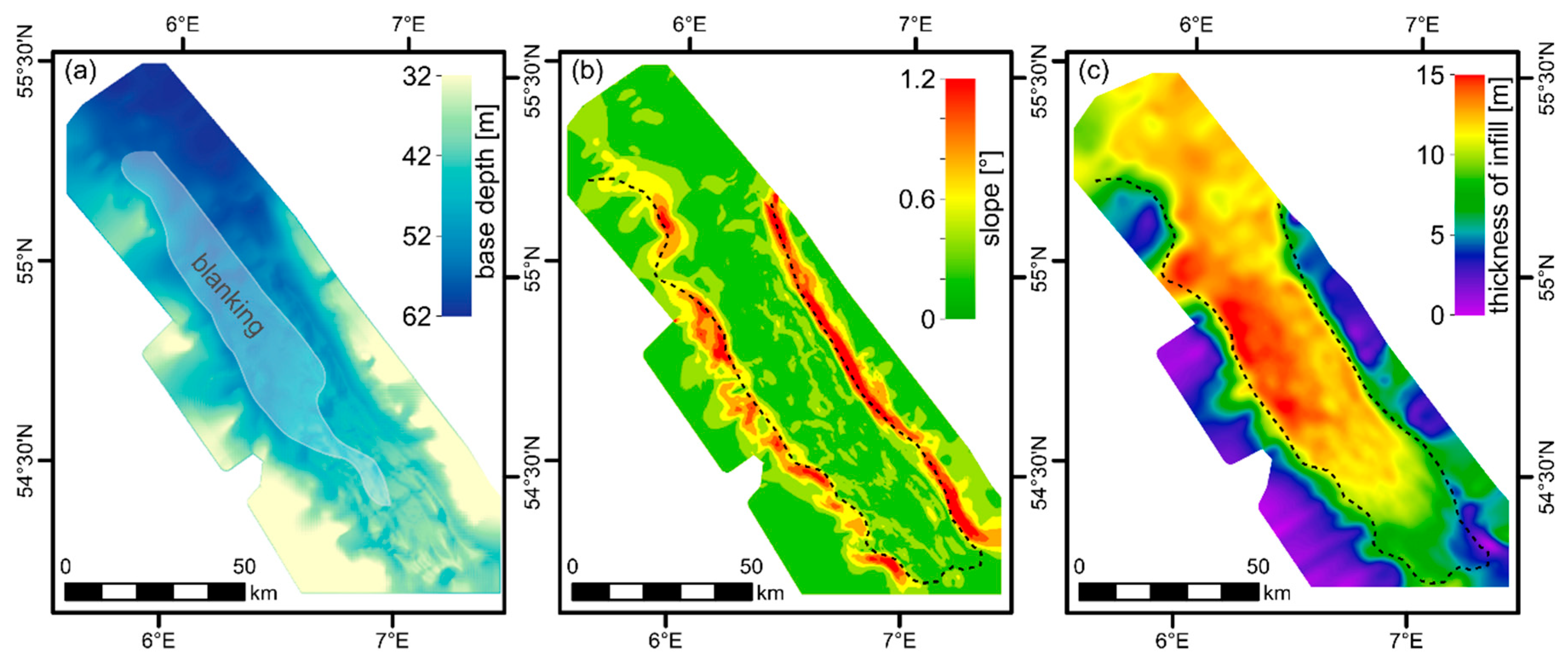
5.1. Valley Geomorphology

The general course and depth of the basin was similar to that described by Figge [5] and could be extended towards the north. The valleys’ bottom was outlined by seismic reflector SR-A (Figure 2). The geographical course of the eastern shore was defined by a Geest landscape formed by moraine ridges of Pleistocene glaciations, which are still present at the sediment surface [10,11,30,50,51,52]. The western shore ended in a flat seafloor, which can be followed closely to the East Frisian coast [5]. Hitherto, studies described the eastern shore to be significantly steeper than the western. However, the area-wide comprehensive data set of this work shows that the slope of the two shores did not differ much. There were just more apparent variations in the slope angle on the eastern shore because of small bays along the margin, which are now delineated by the new data set (Figure 3b). The bay at the eastern margin was postulated by Figge [5] as a tributary system that is possibly related to the present Eider River, which drains the state Schleswig-Holstein in northern Germany. A connection to the present Elbe River was no longer present. During the Holocene, the base of the Paleo Elbe between the present river mouth and Heligoland was, as expected, reworked by waves and currents.
In large areas, the seismic reflector of the central basin (SR-A) and the overlying SU-2 were often blank due to the presence of shallow gas (Figure 2). Indications for gas seepage such as gas flares were not observed while seismic surveying. There was also no indication of pockmarks in backscatter data recorded across the PEV by Papenmeier and Hass [53]. Gas seepage and a large pockmark field were described by Krämer et al. [54] close to the PEV. They speculated that the gas is of biogenic origin from microbial decomposition of postglacial deposits or of thermogenic origin. Both are likely for the PEV. The presence of basal peats was described for other ancient rivers such as the Eider and Ems [54] and salt structures are known south of the study area [55].
Even if the course of individual drainage channels cannot be reconstructed, the low slope gradient along the talweg (10 times lower than the present Elbe), the width of the valley, and its rough morphology lead us to suppose that the discharge of the meltwater occurred in a meandering or braided river channel system that incised the reflector SR-A. The base of the central basin and the river channels could not be sampled by this study. From other studies, it is known that the base consists of Pleistocene sediments [5,6] and the river channels are filled with fluvial sands [6]. However, sedimentological characteristics likely change towards the shores with increasing height relative to the basin. At coring station 4 the base reflector SR-A and the underlying seismic unit SU-1, represented by pale brownish fine sands, could be sampled (Figure 2 and Figure 7). The fine skewed to symmetric, well-sorted, and leptokurtic grain-size distribution suggested a high energetic deposition environment (Figure 9 and Figure 10). These sediments most likely represent supralittoral conditions with aeolian influence, which is powerful in sediment sorting. The theory of a terrigenous sedimentation environment is promoted by the presence of organic remains and missing shells. A riverine origin is unlikely because the sampling depth of the sediments (~46–47 m b.p.s.l.) was about 10 m above the central valley basin where the erosional discharge channels were located. Although a direct age could not be determined, the sediments are older than 9.8 cal. ka BP, which was dated close to the base of SU-2, approximately 10 cm above the upper boundary of SU-1 (Figure 2g). Assuming that the samples were deposited above sea level, they have to be even older than 10.2 cal. ka BP, following the RSL curve for the northern PEV published by Vink et al. [20] (Figure 12). Further to the north, south of the Dogger Bank at a sampling site which was about 10 m below our site, the marine inundation happened around 11 cal. ka BP [6]. Furthermore, according to the RSL of Vink et al. [20], the bottom of the basin (45–62 m b.p.s.l.) would have been flooded completely before 10 cal. ka BP. However, the PEV formed a large bay similar in size to the present Bristol Channel in the United Kingdom, and the complete valley, including the shores (minimum depth 32 m b.p.s.l.), was completely flooded around 9 cal. ka BP [19,20].
Today, the valley is filled up with sediments described by SU-2, SU-3, and SU-4. Grain-size parameters and seismic data indicated changes in the depositional paleoenvironment during sedimentation infill and with increasing sea level, which is described in more detail in the next sections.

5.2. Shallow Marine Conditions

The change from a terrigenous to a marine environment at coring site 4 can be described at a core depth of 4.6 m (Figure 8). The abrupt change in grain size and sediment color at the upper boundary indicates that parts of the stratigraphy are missing, which was probably eroded during a storm surge or when the coring site was inundated by water coming from the north. The first two clay layers at the base of SU-2 (Figure 8) can interpreted as accumulations of low energetic conditions such as tidal or subtidal environments or as mud accumulated after storm surges. Konradi [6] described microfossil assemblages, which are associated with tidal or subtidal conditions at the beginning of the marine inundation. Following this interpretation, this means that for coring station 4 that the sea level had to be at the level of deposition depth (47.2 m b.p.s.l.). The occurrence of shell fragments in the layer indicates a marine influence. Up to the depth of the third peak (4.02 m core depth, ~44 m b.p.s.l.) the sediments were better sorted than the overlying sediments. Likely the valley shores were not yet flooded and the sediments originated from reworked riverine or beach sediments from the valley.
The mean grain size of the third peak (very fine sand) was not as fine as the other two and had a similar size as the main, overlying silty infill of the valley (Figure 8). This was possibly the first, temporal flooding of the valley shores and a sediment input came from the southwest. The shore at the coring site was finally flooded when the RSL was about 40 m below the present. Considering the northern PEV curve of Vink et al. [20], this was around 9.6 cal. ka BP (Figure 12). Afterward, an abrupt change in grain size distribution and characteristics occurred (Figure 8). However, the lower section of SU-2 was not differentiable in the seismic data from the overlying sediments. Possibly the lower part can be interpreted as estuarine sequence, but microfossil analysis is necessary for clarification. Noticeable is the large-scale absence of massive estuarine deposits as commonly known from other drowned shelf paleo valleys [56,57,58]. The large-scale absence in the PEV implies either that estuarine sediments were never deposited or not preserved. Considering the fact that no erosional surface existed between SU-1 and SU-2 and that sea level rise was quite fast, it is likely that estuarine sediments were only deposited in a small amount.

5.3. Wind-/Wave-Driven Sedimentation

With the flooding of the western shore, the sediment source changed and the infill of the valley started. The southwestern sediment input became apparent in the northeast dipping stratigraphy (Figure 2), eastward sediment fining, and a stronger kurtosis of grain-size distribution with increasing transport distance towards the valley center (Figure 10 and Figure 11). Further, the thickness of the prograding and upward coarsening sediment deposits decreased towards the center. Sediments came from the southwest of the PEV lowlands, which are now covered by shallow waters. High mean annual bed shear stress at the beginning of the Holocene, associated with sediment erosion, was modeled by Neill et al. [22]. Suspended sediment transport was mainly induced by wind waves, whereas southwesterly storms had the highest contribution to the net sediment transport [26]. Tidal shear stress had a minor role, particularly as the amphidromic point was close to the study area [25].
The sedimentation rate changed within seismic unit SU-2 on vertical and lateral scales but was generally high (Table 5). Maximum rates of 1.4–1.8 cm per year were calculated between 9.3 and 9.0 cal. ka BP. Around 9.3 cal. ka BP an abrupt cooling event on the Northern Hemisphere is known to have happened from Greenland ice cores [59]. Increased temperature gradients may have driven storm strength and frequency, and thus promoted increased sediment input into the valley. During 9.3 and 9.0 cal. ka BP sedimentation rate was higher than the sea-level rise, leading to a local decrease in water depth (Figure 13). The sedimentation rate was too high to give organisms enough time to settle. This explains why the sediments were almost free of bioturbation and shell fragments.
Around 9 cal. ka BP, when the complete PEV was flooded, including the shores, sedimentation rates decreased and water depth increased again. Benthic organisms had enough time to settle, which was evident in bioturbation and shell fragments. The strongest bioturbation occurred at coring station 1, which explains the lesser upward coarsening compared to station 2, given that bioturbation blends the grain-size trend. Moreover, bioturbation resulted in less clear seismic reflectors at station 1.
The major sediment transport by wind and wave events remained at least until 8165 cal. yr BP (almost the entire SU-2; Figure 2g). Relatively high variability in mean grain size in the short term shows that the energy environment changed regularly. A second northern hemispheric cooling event is known to have happened around 8.2 cal. ka BP, inducing increased storminess [60]. This event was related to the perturbation of the Atlantic Meridional Overturning Circulation caused by the sudden drainage of the Laurentide proglacial lakes Agassiz and Ojibway through the Hudson Strait into the North Atlantic. Strong sand accretion by wind was described in Denmark, for example [61].

5.4. Tide-Driven Sedimentation

At 8.1 cal. ka BP, the western part of the valley was almost filled up, while SU-2 had not reached the eastern shore (Figure 2, Figure 4, and Figure 6). From 8.1 cal. ka BP (RSL 23 m) sedimentation started in the eastern part (SU-3). Meanwhile, the English Channel had opened [16], the tidal system was developed, and bed shear stress through wind and waves decreased because of the increasing water level [25,26]. The Dogger Bank was almost flooded and provided a new sediment source [18]. At 8.15 cal. ka BP, the Storrega tsunami severely impacted wide parts of the North Sea [17], but remained not detectable in the grain size and seismic data of this study.
The decisive environmental change for SU-3 was the development of a tidal system. In the beginning the tidal power was likely too weak to cause a tidal ravinement surface. With increasing tidal power, a consistent, non-event-related, tidal-induced bed shear stress led to a sediment transport as bed load from the flooded lowlands west of the valley and a uniform accumulation within the valley [25]. This explains the missing seismic reflections in the southern part of the valley and the relatively low variability in mean grain size compared to SU-2, although an upward fining persisted. The sedimentation rate was reduced (0.1 m/century) at coring station 1 but had to be higher in the eastern part of the valley, estimated at ca. 0.4 m per century (12 m within 3.1 ka).
The thickness of SU-3 increased northwards, which is related to the morphology of the valley. However, the seismic characteristics also changed northwards. The overall transparent unit (SU-3) was interrupted by single seismic reflectors in the central valley, which strengthened northwards. In the very north, seismic data resemble the linear, storm-induced reflections of SU-2 without any transparent interception. Likely, these sediments were accumulated during severe storm events coming from southwest to northwest without reaching the southern part of the valley.

5.5. Present Mobile Sediment Layer

At approximately 5.0 ka BP, with lower rates of sea-level rise, the sedimentary infill of the PEV was nearly complete. Generally, the uppermost unit (SU-4) was less than 5 m thick (Figure 4c). At the coring stations close to the western shore, the seismic reflector describing the lower limit of SU-4 (SR-G) coincided with a layer of shell fragments. This layer seemed to be a widespread phenomenon in the North Sea, describing a mega-storm or flood event [12,62]. The overlying fine sands showed no distinct internal structures and were interpreted as the mobile sediment layer, as described by Zeiler et al. [28]. The mobile sands get reworked by tidal currents and during storms.
Cross-valley grain-size parameters of the surface shown in Figure 11 indicated an inverse trend compared to the subjacent older sediments. For example, the two eastern coring stations (1 and 2) were coarser than the western ones (3 and 4). This seemed to be a local phenomenon and was not reflected by the general trend of the surface sediments of the complete PEV. Surface grab samples taken across the PEV showed the same trend of sediment fining from west to east as the subsurface samples of coring station 1–4 [31,32,62].

6. Conclusions

A dense, shallow seismic data set and high-resolution grain-size data made it possible to shed new light on the Holocene development of the Paleo Elbe Valley (PEV). The principal course and depth of preceding studies could be reconstructed and extended with more details. The shape of the western shore is more complex through small bays, and the connection to the Paleo-Ems and Elbe can be guessed.
The first indication of marine environment within the cores was found around 9.8 cal. ka BP, approximately 10 m above the basin base. Underneath are moderately well-sorted fine sands probably deposited in a supralittoral environment. At the beginning of inundation, tidal flats dominated the coring site.
The sedimentary infill started when the western shore was flooded (~9.6 cal. ka BP) and can be divided into two major phases. During the first phase (9.6–8.1 cal. ka BP), represented by SU-2, the sedimentation rate was high (up to 1.8 cm per year) and the western part of the valley was filled up. The sediments were eroded and transported from the shallow flooded lowlands southwest of the PEV. Relative high variability in grain size and prograding, densely layered seismic reflectors indicate that the sediment transport and accumulation were wind and wave triggered.
During the second phase (8.1–5.0 cal. ka BP), represented by SU-3, the eastern PEV was filled. The sedimentation was mainly tide driven in the southern part of the valley. In the northern part, seismic data indicate similar characteristics as the layered SU-2 under storm influence. The erosional extent of the previous tidal accumulation remains unknown. Around 5.0 cal. ka BP, the PEV was almost leveled with up to 15 m thick Holocene deposits. The uppermost layer (SU-4) is relatively thin (< 5 m) and is interpreted as analogous to modern mobile sands, which are nowadays regularly reworked during storm events and are known for wide parts of the southern North Sea.
To summarize, this study shows that the infill of the PEV is not comparable in all details with the ordinary transgressive sequence of other drowned shelf paleo valleys. Estuarine deposits, typically dominating the filling of paleo valleys, are largely missing in the PEV. Further, the sediment input came from the valley side and not from the seaward or landward side. This knowledge and the understanding of the depositional controlling factors (storm and tide) during the Holocene transgression helps to validate past environmental modelling studies and to predict the development of modern coastal lowlands with increasing sea level.

Author Contributions

Conceptualization, S.P. and H.C.H.; methodology, S.P. and H.C.H.; formal analysis, S.P. and H.C.H.; investigation, S.P. and H.C.H.; writing—original draft preparation, S.P.; writing—review and editing, S.P.; visualization, S.P. and H.C.H.; funding acquisition, H.C.H. and S.P. All authors have read and agreed to the published version of the manuscript.

Funding

This research was funded by the AMIN I–III project, a research and development cooperation between the Alfred Wegener Institute Helmholtz Centre for Polar and Marine Research and the Federal Maritime and Hydrographic Agency in Hamburg (BSH) [Grant no. 10038521]. It is part of the SedAWZ project coordinated by the BSH and financed by the Federal Agency for Nature Conservation (BfN).

Acknowledgments

We thank the captain and crew of RV Heincke for their support during our research surveys. We thank our student assistants for their help during the surveys and grain-size analysis. Special thanks go to the colleagues of the Geology Section of the IOW for intense discussions. This manuscript is dedicated to my co-author and fantastic colleague H. Christian Hass (thank you). Sadly, he could not live to see the publication of this work.

Conflicts of Interest

The authors declare no conflict of interest.

References

  1. Pratje, O. Dfie Deutung der Steingründe in der Nordsee als Endmoräne. Deutsche Hydrographische Zeitschrift 1951, 4, 106–114. [Google Scholar] [CrossRef]
  2. Hepp, D.A.; Hebbeln, D.; Kreiter, S.; Keil, H.; Bathmann, C.; Ehlers, J.; Mörz, T. An east-west-trending Quaternary tunnel valley in the south-eastern North Sea and its seismic-sedimentological interpretation. J. Quat. Sci. 2012, 27, 844–853. [Google Scholar] [CrossRef]
  3. Lohrberg, A.; Schwarzer, K.; Unverricht, D.; Omlin, A.; Krastel, S. Architecture of tunnel valleys in the southeastern North Sea: New insights from high-resolution seismic imaging. J. Quat. Sci 2020, 35, 892–906. [Google Scholar] [CrossRef]
  4. Ehlers, J.; Grube, A.; Stephan, H.-J.; Wansa, S. Pleistocene Glaciations of North Germany—New Results. In Developments in Quaternary Sciences; Elsevier: Amsterdam, The Netherlands, 2011; Volume 15, pp. 149–162. ISBN 978-0-444-53447-7. [Google Scholar]
  5. Figge, K. Das Elbe-Urstromtal im Bereich der Deutschen Bucht (Nordsee). Eiszeitalter und Gegenwart 1980, 30, 203–211. [Google Scholar] [CrossRef]
  6. Konradi, P.B. Biostratigraphy and environment of the Holocene marine transgression in the Heligoland Channel, North Sea. Bull. Geol. Soc. Denmark 2000, 47, 71–79. [Google Scholar]
  7. Özmaral, A. Climatically Controlled Sedimentary Processes on Continental Shelves. Master’s Thesis, University of Bremen, Bremen, Germany, April 2017. [Google Scholar]
  8. Papenmeier, S.; Hass, H.C. The paleo Elbe River: 10.000 yrs after flooding. In Proceedings of the GEOHAB–Marine Geological and Biological Habitat Mapping, Saint-Petersburg, Russia, 13–17 May 2019. [Google Scholar]
  9. Papenmeier, S.; Hass, H.C. High-resolution area-wide sea-floor mapping: The paleo Elbe valley (S North Sea) revisited. In Proceedings of the Geophysical Research Abstracts; EGU—European General Assembly, Vienna, Austria, 27 April–2 May 2014; EUG2014-11717-1. Volume 16. [Google Scholar]
  10. Diesing, M.; Schwarzer, K. Identifications of submarine hard-bottom substrates in the German North Sea and Baltic EEZ with high-resolution acoustic seafloor imaging. In Progress in Marine Conservation in Europe: Natura 2000 Sites in German Offshore Waters; Springer: Berlin, Heidelberg, 2006; pp. 111–125. [Google Scholar]
  11. Papenmeier, S.; Hass, H. Detection of Stones in Marine Habitats Combining Simultaneous Hydroacoustic Surveys. Geosciences 2018, 8, 279. [Google Scholar] [CrossRef] [Green Version]
  12. Hepp, D.A.; Romero, O.E.; Mörz, T.; De Pol-Holz, R.; Hebbeln, D. How a river submerges into the sea: A geological record of changing a fluvial to a marine paleoenvironment during early Holocene sea level rise. J. Quat. Sci. 2019, 34, 581–592. [Google Scholar] [CrossRef] [Green Version]
  13. EMODnet Digital Terrain Model for European Sea Regions. 2020. Available online: https://portal.emodnet-bathymetry.eu (accessed on 3 November 2020).
  14. Sturt, F.; Garrow, D.; Bradley, S. New models of North West European Holocene palaeogeography and inundation. J. Archaeol. Sci. 2013, 40, 3963–3976. [Google Scholar] [CrossRef] [Green Version]
  15. Cohen, K.M.; Westley, K.; Erkens, G.; Hijma, M.P.; Weerts, H.J.T. The North Sea. In Submerged Landscapes of the European Continental Shelf; Flemming, N.C., Harff, J., Moura, D., Burgess, A., Bailey, G.N., Eds.; John Wiley & Sons, Ltd.: Oxford, UK, 2017; pp. 147–186. ISBN 978-1-118-92782-3. [Google Scholar]
  16. Waller, M.P.; Long, A.J. Holocene coastal evolution and sea-level change on the southern coast of England: A review. J. Quat. Sci. 2003, 18, 351–359. [Google Scholar] [CrossRef]
  17. Gaffney, V.; Fitch, S.; Bates, M.; Ware, R.L.; Kinnaird, T.; Gearey, B.; Hill, T.; Telford, R.; Batt, C.; Stern, B.; et al. Multi-Proxy Characterisation of the Storegga Tsunami and Its Impact on the Early Holocene Landscapes of the Southern North Sea. Geosciences 2020, 10, 270. [Google Scholar] [CrossRef]
  18. Fitch, S.; Thomson, K.; Gaffney, V. Late Pleistocene and Holocene depositional systems and the palaeogeography of the Dogger Bank, North Sea. Quat. Res. 2005, 64, 185–196. [Google Scholar] [CrossRef]
  19. Behre, K.-E. A new Holocene sea-level curve for the southern North Sea. BOREAS 2007, 36, 82–102. [Google Scholar] [CrossRef]
  20. Vink, A.; Steffen, H.; Reinhardt, L.; Kaufmann, G. Holocene relative sea-level change, isostatic subsidence and the radial viscosity structure of the mantle of northwest Europe (Belgium, the Netherlands, Germany, southern North Sea). Quat. Sci. Rev. 2007, 26, 3249–3275. [Google Scholar] [CrossRef]
  21. Baeteman, C.; Waller, M.; Kiden, P. Reconstructing middle to late Holocene sea-level change: A methodological review with particular reference to ‘A new Holocene sea-level curve for the southern North Sea’ presented by K.-E. Behre: Reconstructing middle to late Holocene sea-level change. Boreas 2011, 40, 557–572. [Google Scholar] [CrossRef]
  22. Neill, S.P.; Scourse, J.D.; Uehara, K. Evolution of bed shear stress distribution over the northwest European shelf seas during the last 12,000 years. Ocean. Dyn. 2010, 60, 1139–1156. [Google Scholar] [CrossRef]
  23. Shennan, I.; Lambeck, K.; Flather, R.; Horton, B.; McArthur, J.; Innes, J.; Lloyd, J.; Rutherford, M.; Wingfield, R. Modelling western North Sea palaeogeographies and tidal changes during the Holocene. Geol. Soc. Lond. Spec. Publ. 2000, 166, 299–319. [Google Scholar] [CrossRef]
  24. Uehara, K.; Scourse, J.D.; Horsburgh, K.J.; Lambeck, K.; Purcell, A.P. Tidal evolution of the northwest European shelf seas from the Last Glacial Maximum to the present. J. Geophys. Res. 2006, 111, C09025. [Google Scholar] [CrossRef] [Green Version]
  25. Van der Molen, J.; de Swart, H.E. Holocene tidal conditions and tide-induced sand transport in the southern North Sea. J. Geophys. Res. 2001, 106, 9339–9362. [Google Scholar] [CrossRef]
  26. Van der Molen, J.; de Swart, H.E. Holocene wave conditions and wave-induced sand transport in the southern North Sea. Cont. Shelf Res. 2001, 21, 1723–1749. [Google Scholar] [CrossRef]
  27. Ward, S.L.; Neill, S.P.; Scourse, J.D.; Bradley, S.L.; Uehara, K. Sensitivity of palaeotidal models of the northwest European shelf seas to glacial isostatic adjustment since the Last Glacial Maximum. Quat. Sci. Rev. 2016, 151, 198–211. [Google Scholar] [CrossRef] [Green Version]
  28. Zeiler, M.; Schulz-Ohlberg, J.; Figge, K. Mobile sand deposits and shoreface sediment dynamics in the inner German Bight (North Sea). Mar. Geol. 2000, 170, 363–380. [Google Scholar] [CrossRef]
  29. Wolters, S.; Zeiler, M.; Bungenstock, F. Early Holocene environmental history of sunken landscapes: Pollen, plant macrofossil and geochemical analyses from the Borkum Riffgrund, southern North Sea. Int. J. Earth Sci. (Geol Rundsch) 2010, 99, 1707–1719. [Google Scholar] [CrossRef]
  30. Papenmeier, S.; Galvez, D.; Günther, C.-P.; Pesch, R.; Propp, C.; Hass, H.C.; Schuchardt, B.; Zeiler, M. Winnowed gravel lag deposits between sandbanks in the German North Sea. In Seafloor Geomorphology as Benthic Habitat; Elsevier: Amsterdam, The Netherlands; Oxford, UK; Cambridge, MA, USA, 2020; pp. 451–460. ISBN 978-0-12-814960-7. [Google Scholar]
  31. Papenmeier, S.; Hass, H.C.; Valerius, J.; Thiesen, M.; Mulckau, A. Map of sediment distribution in the German EEZ (1:10.000). 2019. Available online: www.geoseaportal.de/mapapps/rescources/apps/sedimentverteilung_auf_dem_meeresboden/index.html?lang=de (accessed on 3 November 2020).
  32. Callies, U.; Gaslikova, L.; Kapitza, H.; Scharfe, M. German Bight residual current variability on a daily basis: Principal components of multi-decadal barotropic simulations. Geo-Mar. Lett 2017, 37, 151–162. [Google Scholar] [CrossRef] [Green Version]
  33. Sündermann, J.; Pohlmann, T. A brief analysis of North Sea physics. Oceanologia 2011, 53, 663–689. [Google Scholar] [CrossRef] [Green Version]
  34. Zeiler, M.; Milbrandt, P.; Plüß, A.; Valerius, J. Modelling large scale sediment transport in the German Bight (North Sea). Die Küste 2014, 81, 369–392. [Google Scholar]
  35. Hass, H.C.; Papenmeier, S. Parametric Sediment Echo Sounder Survey during R/V Heincke Cruise HE400 in the German Bight with Link to Raw Data Files; Alfred Wegener Institute—Wadden Sea Station Sylt, PANGAEA: Bremerhaven, Germany, 2019. [Google Scholar] [CrossRef]
  36. Papenmeier, S.; Hass, H.C. Parametric Sediment Echo Sounder Survey during R/V Heincke Cruise HE415 and HE416 in the German Bight with Link to Raw Data Files; Alfred Wegener Institute—Wadden Sea Station Sylt, PANGAEA: Bremerhaven, Germany, 2019. [Google Scholar] [CrossRef]
  37. Papenmeier, S.; Hass, H.C. Parametric Sediment Echo Sounder Survey during R/V Heincke Cruise HE436 in the German Bight with Link to Raw Data Files; Alfred Wegener Institute—Wadden Sea Station Sylt, PANGAEA: Bremerhaven, Germany, 2019. [Google Scholar] [CrossRef]
  38. Papenmeier, S.; Hass, H.C. Parametric Sediment Echo Sounder Survey during R/V Heincke Cruise HE438 in the German Bight with Link to Raw Data Files; Alfred Wegener Institute—Wadden Sea Station Sylt, PANGAEA: Bremerhaven, Germany, 2019. [Google Scholar] [CrossRef]
  39. Wunderlich, J.; Wendt, G.; Müller, S. High-resolution Echo-sounding and Detection of Embedded Archaeological Objects with Nonlinear Sub-bottom Profilers. Mar. Geophys Res. 2005, 26, 123–133. [Google Scholar] [CrossRef]
  40. Wunderlich, J.; Müller, S.; Hümbs, P.; Buch, T.; Endler, R. High-Resolution Acoustical Site Exploration in Very Shallow Water—A Case Study. In Proceedings of the EAGE Near Surface 2005—11th European Meeting of Environmental and Engineering Geophysics, Palermo, Italy, 4–7 September 2005; European Association of Geoscientists & Engineers: Amsterdam, The Netherlands, 2005; pp. 1–4. [Google Scholar]
  41. Hass, H.C.; Kuhn, G.; Monien, P.; Brumsack, H.-J.; Forwick, M. Climate fluctuations during the past two millennia as recorded in sediments from Maxwell Bay, South Shetland Islands, West Antarctica. Geol. Soc. Lond. Spec. Pub. 2010, 344, 243–260. [Google Scholar] [CrossRef]
  42. Folk, R.L.; Ward, W.C. Brazos River bar [Texas]; a study in the significance of grain size parameters. J. Sediment. Res. 1957, 27, 3–26. [Google Scholar] [CrossRef]
  43. Blott, S.J.; Pye, K. GRADISTAT: A grain size distribution and statistics package for the analysis of unconsolidated sediments. Earth Surf. Process. Landf. 2001, 26, 1237–1248. [Google Scholar] [CrossRef]
  44. Reimer, P.J.; Bard, E.; Bayliss, A.; Beck, J.W.; Blackwell, P.G.; Ramsey, C.B.; Buck, C.E.; Cheng, H.; Edwards, R.L.; Friedrich, M.; et al. IntCal13 and Marine13 Radiocarbon Age Calibration Curves 0–50,000 Years cal BP. Radiocarbon 2013, 55, 1869–1887. [Google Scholar] [CrossRef] [Green Version]
  45. Hass, H.C.; Papenmeier, S. Documentation of Sediment Core HE439/06-1 (HE438-439_EUT1); Alfred Wegener Institute—Polarstern Core Repository, PANGAEA: Bremerhaven, Germany, 2015. [Google Scholar] [CrossRef]
  46. Hass, H.C.; Papenmeier, S. Documentation of Sediment Core HE439/07-1 (HE438-439_EUT2); Alfred Wegener Institute—Polarstern Core Repository, PANGAEA: Bremerhaven, Germany, 2015. [Google Scholar] [CrossRef]
  47. Hass, H.C.; Papenmeier, S. Documentation of sediment core HE439/08-1 (HE438-439_EUT3); Alfred Wegener Institute—Polarstern Core Repository, PANGAEA: Bremerhaven, Germany, 2015. [Google Scholar] [CrossRef]
  48. Hass, H.C.; Papenmeier, S. Documentation of Sediment Core HE439/09-1 (HE438-439_EUT4); Alfred Wegener Institute—Polarstern Core Repository, PANGAEA: Bremerhaven, Germany, 2015. [Google Scholar] [CrossRef]
  49. Galvez, D.S.; Papenmeier, S.; Hass, H.C.; Bartholomae, A.; Fofonova, V.; Wiltshire, K.H. Detecting shifts of submarine sediment boundaries using side-scan mosaics and GIS analyses. Mar. Geol. 2020, 430, 106343. [Google Scholar] [CrossRef]
  50. Michaelis, R.; Hass, H.C.; Mielck, F.; Papenmeier, S.; Sander, L.; Gutow, L.; Wiltshire, K.H. Epibenthic assemblages of hard-substrate habitats in the German Bight (south-eastern North Sea) described using drift videos. Cont. Shelf Res. 2019, 175, 30–41. [Google Scholar] [CrossRef]
  51. Michaelis, R.; Hass, H.C.; Mielck, F.; Papenmeier, S.; Sander, L.; Ebbe, B.; Gutow, L.; Wiltshire, K.H. Hard-substrate habitats in the German Bight (South-Eastern North Sea) observed using drift videos. J. Sea Res. 2019, 144, 78–84. [Google Scholar] [CrossRef]
  52. Papenmeier, S.; Hass, H.C. Sidescan Sonar Survey (300 / 600 kHz) during R/V Heincke Cruise HE436 in the German Bight with Link to Raw Data Files; 111.3 GBytes; PANGAEA Alfred Wegener Institute—Wadden Sea Station Sylt: Bremerhaven, Germany, 2019. [Google Scholar] [CrossRef]
  53. Krämer, K.; Holler, P.; Herbst, G.; Bratek, A.; Ahmerkamp, S.; Neumann, A.; Bartholomä, A.; van Beusekom, J.E.E.; Holtappels, M.; Winter, C. Abrupt emergence of a large pockmark field in the German Bight, southeastern North Sea. Sci. Rep. 2017, 7, 5150. [Google Scholar] [CrossRef]
  54. Sindowski, K.-H. Das Quartär im Untergrund der Deutschen Bucht (Nordsee). Eiszeitalter und Gegenwart 1970, 21, 33–46. [Google Scholar]
  55. Allen, G.P.; Posamentier, H.W. Sequence Stratigraphy and Facies Model of an Incised Valley Fill: The Gironde Estuary, France. SEPM J. Sediment Res. 1993, 63. [Google Scholar] [CrossRef]
  56. Wei, X.; Wu, C. Holocene delta evolution and sequence stratigraphy of the Pearl River Delta in South China. Sci. China Earth Sci. 2011, 54, 1523–1541. [Google Scholar] [CrossRef]
  57. Hewlett, R.; Bimie, J. Holocene environmental change in the inner Severn estuary, UK: An example of the response of estuarine sedimentation to relative sea-level change. The Holocene 1996, 6, 49–61. [Google Scholar] [CrossRef]
  58. Vinther, B.M.; Clausen, H.B.; Johnsen, S.J.; Rasmussen, S.O.; Andersen, K.K.; Buchardt, S.L.; Dahl-Jensen, D.; Seierstad, I.K.; Siggaard-Andersen, M.-L.; Steffensen, J.P.; et al. A synchronized dating of three Greenland ice cores throughout the Holocene. J. Geophys. Res. 2006, 111, D13102. [Google Scholar] [CrossRef]
  59. Clarke, M.L.; Rendell, H.M. The impact of North Atlantic storminess on western European coasts: A review. Quat. Int. 2009, 195, 31–41. [Google Scholar] [CrossRef]
  60. Dalsgaard, K.; Vad Odgaard, B. Dating sequences of buried horizons of podzols developed in wind-blown sand at Ulfborg, Western Jutland. Quat. Int. 2001, 78, 53–60. [Google Scholar] [CrossRef]
  61. Uffenorde, H. Zur Gliederung des klastischen Holozäns im mittleren und nordwestlichen Teil der Deutschen Bucht (Nordsee) unter besonderer Berücksichtigung der Foraminiferen. E&G—Quat. Sci. J. 1982, 32, 177–202. [Google Scholar] [CrossRef]
  62. Papenmeier, S.; Hass, H.C. Grain-Size Properties of Grab-Sampled Sediments from the German Bight during R/V Heincke Cruise HE436; PANGAEA Alfred Wegener Institute—Wadden Sea Station Sylt: Bremerhaven, Germany, 2019. [Google Scholar] [CrossRef]
Figure 1. Overview map showing the study area. (a) Bathymetry from the present North Sea of the EMODnet data portal [13] with the course of the paleo Elbe valley (PEV) predicted by Konradi [6]. The study site is marked by the blue polygon. (b) Study site with backscatter data for the PEV and the western Sylter Outer Reef modified after Papenmeier and Hass [11]. Parametric sediment echosounder (pSES) data exist for all backscatter data (HE400, H415, HE436) and for cruise HE438 (green lines). Profiles 1–3 represent the cross-sections of Figure 2. Coring stations 1–4 are along profile 1.
Geosciences 10 00505 g001
Figure 2. Cross profiles 1–3 of the PEV. For location see Figure 1. (ac) Parametric sediment echo sounder profiles, (df) interpreted seismic units (SU), and (g) detail of profile 1 with some highlighted seismic reflectors (SR) and AMS 14C age determination (cal. yr BP).
Geosciences 10 00505 g002
Figure 3. (a) Depth of the PEV below present sea level (reflector SR-A), (b) slope of the PEV, and (c) thickness of the sedimentary infill (seismic unit SU-2, 3 and 4). The dashed line represents the outline of the basin.
Geosciences 10 00505 g003
Figure 4. Thickness of the seismic units SU-2 (a), SU-3 (b), and SU-4 (c). Values were not calculated for the northern part of the valley because the density of data was lower and reliable identification of the seismic reflectors was more difficult.
Geosciences 10 00505 g004
Figure 5. Depth of distinct seismic reflectors representing the upper boundary of seismic units. (a) Top of SU-2 (SR-F) and (b) top of SU-3 (SR-G). Values were not calculated for the northern part of the valley because the density of data was lower and reliable identification of the seismic reflectors was more difficult.
Geosciences 10 00505 g005
Figure 6. A 3-D model of the Paleo Elbe Valley basin and the upper boundary of seismic unit SU-2 (SR-B) and seismic unit SU-3 (SR-G).
Geosciences 10 00505 g006
Figure 7. Photographs of Section 4 and Section 5 (3.35–5.35 m) of core 4. Significant changes in sediment characteristics existed between 4.0 m and 4.6 m.
Geosciences 10 00505 g007
Figure 8. Grain-size analysis for coring sites 1–4. Top (ad): mean grain size with 5-point running mean. The gray boxes represent the different seismic units (SU). The dashed lines represent specific seismic reflectors (SR). Bottom (eh): frequency of size classes.
Geosciences 10 00505 g008
Figure 9. The bivariate plots show the relation between the mean grain size and the sorting for the four seismic units (SU). The colors represent the coring station (1: yellow, 2: red, 3: green, 4: blue). Black dots represent the complete data set (all SU).
Geosciences 10 00505 g009
Figure 10. The bivariate plots show the relation between the skewness and the kurtosis for the four seismic units (SU). The colors represent the coring station (1: yellow, 2: red, 3: green, 4: blue). Black dots represent the complete data set (all SU).
Geosciences 10 00505 g010
Figure 11. Grain size parameters of certain seismic reflectors and the sediment surface calculated after the modified Folk and Ward method [44]. The individual values represent the mean of samples 5 cm above and below the reflector depth.
Geosciences 10 00505 g011
Figure 12. Relative sea-level curve for the southern North Sea modified after Behre [19] and Vink et al. [20] with determined AMS 14C age.
Geosciences 10 00505 g012
Figure 13. Calculated water depth (using the PEV curve of Vink et al. [20] in Figure 12) for the seismic reflectors with age determination.
Geosciences 10 00505 g013
Table 1. Parametric sediment echo sounder (pSES) data sets, settings, and respective databases.
CruiseDatepSES Low FrequencypSES Pulse Length [µs]DOI
HE40005/20136 kHz2doi:10.1594/PANGAEA.899708, [36]
HE41502/201410 kHz2doi:10.1594/PANGAEA.905842, [37]
HE43611/20148 kHz2doi:10.1594/PANGAEA.899707, [38]
HE43802/20158, 15 kHz1, 2doi:10.1594/PANGAEA.899497, [39]
Table 2. Details of core sampling sites. The short number is the number used within the text and figures.
Core NumberShort NumberLatitudeLongitudeRecoveryWater Depth
HE439/006-1154°49.21′ N06°14.77′ E5.98 m39.2 m
HE439/007-1254°48.32′ N06°12.62′ E4.79 m39.4 m
HE439/008-1354°47.85′ N06°11.38′ E5.86 m41.0 m
HE439/009-1454°47.12′ N06°09.60′ E5.42 m41.5 m
Table 3. Details of the AMS 14C age determinations. Sample material was calcareous shell fragments.
Lab CodeCoreSample Depth [cm]Conventional Age [yr BP]Calibrated Age [cal. yr BP] 1
Beta-416333189–904730 ± 305027 ± 177
Beta-4163341425–4267680 ± 308165 ± 125
Beta-4163352400–4028420 ± 309072 ± 112
Beta-4163363454–4568670 ± 309364 ± 104
Beta-4163374454–4559100 ± 309817 ± 277
1 Midpoint of 68% probability range
Table 4. Links to the database with detailed core descriptions and photographs.
Core NumberShort NumberLink to Core Documentation
HE439/006-11https://doi.pangaea.de/10.1594/PANGAEA.847257, [46]
HE439/007-12https://doi.pangaea.de/10.1594/PANGAEA.847258, [47]
HE439/008-13https://doi.pangaea.de/10.1594/PANGAEA.847259, [48]
HE439/009-14https://doi.pangaea.de/10.1594/PANGAEA.847260, [49]
Table 5. Sedimentation rate meter per century for selected periods.
Period [cal. yr BP]Core 3Core 2Core 1
8165–5027--0.1
9072–8165-0.30.4
9364–9072-1.81.4
9817–936410.90.6
Publisher’s Note: MDPI stays neutral with regard to jurisdictional claims in published maps and institutional affiliations.

