Shape and Dimension Estimations of Landslide Rupture Zones via Correlations of Characteristic Parameters

Domej, Gisela; Bourdeau, Céline; Lenti, Luca; Martino, Salvatore; Pluta, Kacper

doi:10.3390/geosciences10050198

Open AccessArticle

Shape and Dimension Estimations of Landslide Rupture Zones via Correlations of Characteristic Parameters

¹

Laboratoire SRO, Département GERS, Université Gustave Eiffel, 14–20 Boulevard Newton, 77447 Marne–la–Vallée, France

²

Laboratoire MouvGS, Centre d’études et d’expertise sur les Risques, l’Environnement, la Mobilité et l’Aménagement, 500 Route des Lucioles, 06903 Valbonne-Sophia Antipolis, France

³

Dipartimento di Scienze della Terra & Centro di Ricerca per i Rischi Geologici, Università Sapienza di Roma, Piazzale Aldo Moro 5, 00185 Rome, Italy

⁴

Computer Science Department, Technion—Israel Institute of Technology, Taub Building, Haifa 3200003, Israel

^*

Author to whom correspondence should be addressed.

Geosciences 2020, 10(5), 198; https://0-doi-org.brum.beds.ac.uk/10.3390/geosciences10050198

Submission received: 7 April 2020 / Revised: 11 May 2020 / Accepted: 12 May 2020 / Published: 21 May 2020

(This article belongs to the Section Natural Hazards)

Download

Browse Figures

Versions Notes

Abstract

:

For many geotechnical purposes, the proper estimation of shapes and dimensions of landslide rupture zones is of significant importance. Very often, this exact delineation is difficult due to the lack of information on rupture zone extents in 3D. Based on a global landslide inventory, this work presents statistical analyses correlating dimension-related and shape-related parameters characterizing a rupture zone in 3D to its volume. Dimension-related parameters are approximated by linear regressions increasing with greater volumes, whereas shape-related parameters appear stable throughout the entire range of volumes. Revealing themselves as very stable, these correlations can be used, hence, to extrapolate from a distinct parameter to the volume of a landslide rupture zone. In a second stage, ratios of dimension-related parameters are correlated with rupture zone volumes. Furthermore, this type of correlation delivers very stable results showing that ratios are constant throughout the entire range of volumes. Making use of this ratio consistency, it is possible to deduce one of the two parameters when the other one is given. This latter aspect seems to be promising for remote sensing surveys when initial rupture areas or rupture volumes should be delineated or for numerical modeling of landslides in 3D.

Keywords:

landslide shape; landslide dimension; rupture zone; landslide size estimation; landslide database

1. Introduction

Across the globe, landslides are triggered by a variety of causes. They regularly lead to loss of life and damage, ranging from smaller to greater extent [1,2]. Common triggers are of tectonic, volcanic, meteorological, and anthropogenic nature or a combination of them [3,4]. As an example illustrating the trail of destruction serves the landslide series triggered during Hurricane Mitch in October 1998, which caused tremendous damage and 2000 fatalities in Nicaragua alone [5]. Another more recent example of devastation is the landslide series after the Sichuan Earthquake in May 2008, with a ten times higher number of victims (20,000) [6].

Over the last decades, major contributions to a better understanding of the phenomenon of landslides in terms of, e.g., geographical localization, area and volume distributions, frequency, and probability analyses, as well as rupture mechanisms, were made by the establishment and consecutive exploration of landslide databases, which could be chronologic (i.e., listing landslides with different triggers over time) or event-based (i.e., listing landslides caused by a particular triggering event). The latter might be tectonic events (e.g., earthquakes, fault ruptures, or volcanic activity), meteorological events (e.g., heavy rain or storms), and climatic changes on a seasonal or long-term scale (e.g., snowmelt or permafrost degradation). Scientific work based on landslide databases with respect to the type of triggering events is exhaustive, and a full overview would be beyond the scope of this publication. Some examples are: studies using global, regional, and event-based databases of earthquake-triggered landslides by Harp and Jibson [7,8], Keefer et al. [9], Prestininzi and Romeo [10], Rodríguez et al. [11], and Tanyaş et al. [12]; studies based on landslide databases related to climatic changes such as snowmelt (e.g., [13]) and general climate change (e.g., [14]); and studies using event-based meteorological databases (e.g., [15]). An even more abundant number of studies on landslide databases became available due to the increasing reliability of remote sensing techniques, which allow for rapid mapping and analyses of single landslides or landslide clusters at different scales all over the globe.

In view of constant population growth and expansion to new and occasionally endangered living environments, proper management of landslide risk is essential for social resilience. In addition, climate change is not to be disdained in this context, as frequency and intensity of extreme meteorological events are expected to increase, which, in turn, can trigger numerous landslides.

Relating to event magnitude and successive consequences, the volume of landslides is considered as one of the most significant parameters [16], which becomes apparent, e.g., when comparing unequal damage potentials of small and frequent events with large and rare events. Exact estimates for landslide volumes are, however, among the most difficult parameters to assess.

Following this essential need for detailed volume assessment of landslides, this publication presents statistical analyses focusing on expected dimensions and shapes of landslide rupture zones in 3D. The term “rupture zone” refers here to the landslide volume that is confined by the rupture surface at the moment of the main rupture event (Figure 1a–d). In contrast to other authors (e.g., [16,17,18,19,20,21,22,23]), who consider landslide zones as the entire zone affected by sliding processes for different purposes (e.g., mapping and inventory work for statistical applications, area-to-volume and area-to-depth correlations, or probability and frequency analyses), this work clearly distinguishes the entire landslide zone from the zone confining the rupture volume of landslides. As the Frank Landslide, Canada (No. 019.00 in Table A1 in the Appendix A), in Figure 2 illustrates, the distinction of both zones implies significant differences in terms of area and volume. Another difference to common landslide inventories is that, here, many more depth-related parameters are available delimiting the rupture zone at different locations, whereas other authors use a single multiplier to account for depth extents (e.g., [24,25,26,27,28]). Both aspects might be of particular interest for application in remote sensing or numerical landslide modeling.

Statistical analyses are based on a newly created chronologic database presented by Domej et al. [31] comprising 277 landslides in 40 countries across the globe (Figure 3), which will be revisited in the first part of this publication. The second part is dedicated to statistical analyses consisting of correlations between landslide volumes and single parameters characterizing landslide rupture zones and of correlations between landslide volumes and ratios of single parameters. The last section discusses results as well as their potential fields of application. All landslides included in the database are listed with their date, location, and trigger in Table A1 in the Appendix A. Initially designed for seismically induced landslides, the database consists majorly, but by far not exclusively, of earthquake-triggered landslides; triggers also range from precipitation, storms, and anthropogenic influence to unknown causes.

2. Statistical Analyses

The analyses aim for a general understanding of the statistical behavior of geometrical parameters characterizing landslide rupture zones (Figure 4) with increasing landslide sizes.

In theory, i.e., if the data coverage is fully exhaustive, a total number of 66 parameters and descriptive notes with respect to longitudinal cross sections (LCS), transversal cross sections (TCS) and top views (maps) are available for each landslide included in the database; they are adapted and further developed from the parameters proposed by the IAEG Commission on Landslides [33]. Individual parameters that are used for the here presented analyses are listed in Table 1 and can be either directly or indirectly derived from available publications. Direct parameters are those that are measured from LCS, TCS, and/or maps published per respective landslide. Indirect parameters are those that are calculated via equations using direct parameters (Table 1). The calculated volume (V_equ) is derived from the equation of Cruden and Varnes [34] as half an ellipsoid (Figure 4) approximating landslides. The curvature—taken as the difference between the angles at points 0 and E (δ₀ and δ_E)—is not an international standard, but was adopted by the authors; the higher the difference is, the higher is the curvature (Figure 4). Being defined via a simple height-over-length-tangent, the calculated slope angle (α_equ) also represents the mean slope angle of the rupture zone (Figure 4). The perspective of the TCS represents a view from the landslide toe towards the landslide crest. An example of the measurements of the parameters characterizing the rupture zone is shown in Figure 5 using the Diezma Landslide, Spain (No. 001.00 in Table A1 in the Appendix A).

Usually, the number of evaluable parameters decreases due to the availability of data throughout the database. For 80% of all landslides in the database, a map is available, for 71% there is an LCS, and for 61% there are both a map and an LCS. Only two of the 277 landslides have an exhaustive TCS record. Therefore, parameters that are derived from the respective imagery show different recurrences. All parameters, except the areas (A and A_h) and the reported slope angle (α_lit), have a recurrence of 70% or higher throughout the database. This ensures sufficient data availability for exactly those parameters that are most interesting to analyze regarding shapes and dimensions of landslide rupture zones, not only superficially, but also with respect to the extent of the depth.

The analyses follow the approach of simple volume-to-parameter correlation and volume-to-ratio correlation (Figure 6). Although being the most complexly interlinked indirect parameter, the calculated volume (V_equ) was chosen as the first variable of correlation, which is justified by its strikingly high recurrence or 74%. The reported volume (V_lit; not used in this work and not mentioned in Table 1), in contrast, has a recurrence of only 60%, and covers in many cases also parts of the deposit volumes which conflicts with the exclusive assessment of the rupture zone. The argument that the equation of Cruden and Varnes [34] is suitable for rotational slides while misestimating volumes of translational and roto translational geometries, could at least in this work be rebutted. Where the reported volume (V_lit) and the calculated volume (V_equ) clearly refer to the rupture zone, comparisons of the two volume types do not indicate a notable difference [31].

2.1. Volume-to-Parameter Correlations

One of the two approaches that allow for statistical analyses of the behavior of dimension- and shape-related parameters consists of volume-to-parameter correlations. One variable of correlation is necessarily the calculated volume (V_equ), whereas the place of the second variable of correlation is taken by any of the parameters characterizing the rupture zone in 3D (Figure 4, Table 1).

Here, the choice of suitable variables of correlation is limited by reflections on sample sizes and meaningfulness. Considering the set “full/landslide only”, sample sizes for different parameters vary as a function of the applied filter cascade (Table 2). The term “landslide” refers here to classic landslides sliding on actual sliding surfaces, not displaying local features of other mass movement types such as rock falls, topples, or earth flows [37]. Thereupon apply the filters for the two variables of correlation as uniquely those landslide records showing the calculated volume (V_equ), as well as the respective parameter of interest, can be used for evaluation (Figure 6). For the shape-related parameters, the calculated slope angle (α_equ), the angles at points 0 to E (δ₀ to δ_E), and the curvature (cur), the thereby obtained sample sizes are very satisfying and vary between 153 and 176 cases (second columns of Table 3 and Table 4). The reported slope angle (α_lit) is to be evaluated for 84 cases, both area types (the reported area (A) and its projection to the horizontal (A_h)) are represented only by 72 cases. All TCS related parameters are quasi-nonrepresented by solely three cases at the maximum and, hence, not considered for the analyses (Table 1). The choice to filter according to rotational (i.e., rather half-elliptical shapes; e.g., Figure 4), translational (i.e., rather flat shapes; e.g., Figure 5) and roto-translational rupture zones is explained by the fact that this information is available for every landslide included in the database. The filter, hence, does not reduce the sample sizes.

As for the reported area (A) and its projection to the horizontal (A_h), one might criticize that despite their good representation, they are not included in the volume-to-parameter correlations. Here the argument is that area reports on landslides are to be seen with caution, especially when it comes explicitly to the delineation of rupture zones. Rupture and runout zones can be overlapping, adjacent, or even separated (Figure 1a–d); very often, reported areas refer to the entire area across a slope, which is affected by the sliding process. For several landslides in the database, the distinction between these different area types is not clear, and thus correlations were dismissed. Another argument is that this very uncertainty might become a field of application of the presented statistical correlations.

In contrast to the sifting of unsuitable variables of correlation, also a few new appropriate parameters were also created. They might become of particular interest when delineating average dimensions of rupture zones rather than maximal possible extents in particular locations of rupture zones.

d_av5: average depth of the rupture zone below points 0, 1, 2, 3, E
d_av4: average depth of the rupture zone below points 0, 1, 2, 3
d_av3: average depth of the rupture zone below points 1, 2, 3
w_av5: average width of the rupture zone at points 0, 1, 2, 3, E
w_av3: average width of the rupture zone at points 1, 2, 3

Expecting variable statistical behaviors throughout dimension and shape-related parameters after initial data cloud inspection, fitting tests of different distribution types were applied to each parameter distribution with MATLAB’s Curve Fitting Tool [32]. It appeared that for the climbing trend-prone dimension-related parameters, the best results were obtained by fittings of linear regressions, i.e., of polynomials of the first degree in double-logarithmic diagrams. For the shape-related parameters visibly lacking a climbing trend, such linear regressions were nevertheless “forced” on data clouds in x-semi-logarithmic diagrams with very unsatisfactory results regarding the fitting (i.e., R² almost 0 and significantly high RMSE). Furthermore, the polynomial factors within these “forced” regressions tended to be low, which emphasized the representation of the respective data clouds by their mean values (µ). Taking into account that both dimension- and shape-related parameters exist within the volume-to-parameter correlations (Table 3 and Table 4), a homogeneous way of analyses had to be adopted. For internal consistency, hence, all distributions of dimension-related parameters underwent the fitting of linear regressions in double-logarithmic diagrams, whereas, for all distributions of shape-related parameters, the mean value (µ) was calculated. Furthermore, the homogeneity of analyses between the concerned volume-to-parameter correlations and the likewise shape-based volume-to-ratio correlations (Table 5; next subsection) was preserved.

In the following, the analytical procedure for the most comprehensive set “full” is described. It should be mentioned beforehand that the identical procedure was carried out also for all other sets (Table 2) in order to observe potential changes in statistical behaviors. A comparison of the results of all six tested sets is given in the discussion.

Regressions are here of the general type

y = 10^a V_equ^b,

(1)

and appear in a double-logarithmic diagram as

log₁₀(y) = a + b·log₁₀(V_equ),

(2)

with y defining the respective parameter, a representing the intercept on the y-axis (herein after called “constant”) and b defining the gradient (herein after called “factor”).

Examples of regression fittings are shown in Figure 7a–c for the set “full” for the maximum depth (D), the height between the point 0 and the point E (H_0E), and the length along the slope (L). Despite different scatter patterns, all data clouds reveal a clear increasing tendency. Regressions fit with a few exceptions with coefficients of determination (R²) above or equal to the typical threshold of acceptance of 0.7 (Table 3). Furthermore, within the other five tested sets (Table 2), all regressions fit with similar coefficients of determination (R²). Thus, regression fitting seems to be an adequate tool for correlating calculated volumes (V_equ) and dimension-related parameters. Results for the set “full” are listed in Table 3. The last two columns give the constant (a) as well as the factor (b) that must be inserted into Equation (2) in order to reproduce the straight line per parameter in the respective double-logarithmic diagram.

Conclusions on dispersion are to be regarded with caution in the case of dimension-related parameters. The main reason is that each point in the data clouds depends only on one value of the calculated volume (V_equ); i.e., there is no option to measure dispersions per distinct volume.

The analytical procedure for shape-related parameters (Table 4) consisted of averaging the values represented by the respective data clouds, since “forced” regression fitting in x-semi-logarithmic diagrams resulted in low factors (b), R² close to 0, and significantly high RMSE (Figure 7d, Table 3). Besides the assumption of consistency throughout different calculated volumes (V_equ), there is also a second strong argument favoring simple value averaging instead of regression fitting. Considering perfectly normally distributed data, specific fractions of it should lie within symmetric belts of two (±1σ), four (±2σ) and six (±3σ) standard deviations around the mean value (µ). In the case of the set “full”, data of the individual shape-related parameters follow these suggested intervals with minor deviations (Table 4). One can assume, hence, that data of shape-related parameters are normally distributed what emphasizes the representativeness of the respective mean value (µ). Also, the other five tested sets (Table 2) reveal very similar tendencies with respect to the required fraction of data within the three symmetric belts; only in six cases, sigma interval thresholds were missed by more than 5%.

An example of averaging values is shown in Figure 7d for the set “full” for the calculated slope angle (α_equ), which shows a slight decreasing tendency for very great calculated volumes (V_equ). This phenomenon is probably due to the fact that slopes cannot become infinitely high. Overall, the mean value (µ) seems, however, representative.

All mean values (µ) are listed in Table 4, together with their standard deviations (σ) and the relations between both types of values (µ/σ) as a measure for dispersion. Here, the information about dispersion is of much bigger interest than the dimension-related parameters.

2.2. Volume-to-Ratio Correlations

The second of the two approaches designed for statistical analyses of the behavior of shape-related parameters consists of volume-to-ratio correlations. From plotting the respective distributions, ratios of dimension-related parameters are assumed to behave like shape-related parameters and can, therefore, be analyzed in a similar way—however, with more sophisticated filtering.

Here, the correlation variable on the y-axis is a ratio of two individual (dimension-related) parameters characterizing the rupture zone in 3D (Figure 4, Table 1); after adding a fifth filter (Table 2), sample sizes for the set “full” are still very high ranging from 146 to 176 (second column of Table 5).

In analogy to the argumentation in the previous subsection, reported areas (A) and their projections to the horizontal (A_h) are less profitable candidates for ratios. This is also the case for separate widths (w₀ to w_E) and depths (d₀ to d_E), as they would result in specific ratios that might not be of great use for application; here, it appeared to be more promising to use the newly defined averaged parameters mentioned in the previous subsection (d_av5, d_av4, d_av3, w_av5, and w_av3) to create meaningful ratios.

With respect to these viewpoints and the aim of not creating ratios within the same types of dimension-related parameters (i.e., between lengths, heights, widths, and depths respectively), and accounting for the difference between maximum (e.g., W) and average parameters (e.g., w_av5), 24 significant ratios were identified (Table 5).

Assuming that ratios behave statistically in the same way as other shape-related parameters, they underwent the same procedure of averaging values in order to keep the overall analyses homogeneous and comparable. Again, ratios reveal themselves as constant, emphasizing the assumption of self-similar shapes of rupture zones throughout different ranges of the calculated volume (V_equ). Similar concepts of self-similarity were proposed, e.g., by Guzzetti et al. [18], Malamud et al. [16], and Stark and Guzzetti [38] with respect to the entire landslide zone (Figure 1a–d).

The same strong argument for the representativeness of the mean value (µ) applies to the volume-to-ratio correlations presented here. Table 5 shows for the set “full” that the fractions of data lie with minor deviations within symmetric belts of two (±1σ), four (±2σ) and six (±3σ) standard deviations around the mean value (µ) indicating normal distributions. Also, the other five tested sets (Table 2) reveal very similar tendencies with respect to the required fraction of data within the three symmetric belts; only in five cases, sigma interval thresholds were missed by more than 5%.

Examples for averaging values are shown in Figure 8a–d for the set “full” for the ratio of the height between the point 0 and the point E to the projected length (H_0E/L_h), the ratio of the average depth to the length along the slope (d_av5/L), the ratio of the average width to the length along the slope (w_av5/L), and the ratio of the average depth to the average width (d_av5/w_av5).

Comparing the four examples, the ratio of the average depth to the length along the slope (d_av5/L) appears as the most dispersed (Figure 8b), although 75.8% of the data points lie still in symmetric belts of two (±1σ) standard deviations around the mean value (µ). The dispersion reflects the fact that rupture zones of landslides appear to be unequal concerning depth, which is a strong argument of not using a simple multiplier when estimating depths of rupture zones and landslides in general.

The other three examples in Figure 8a–d also show good ratio stability throughout the calculated volumes (V_equ). This is particularly interesting for the ratio of the height between the point 0 and the point E to the projected length (H_0E/L_h), as Heim [39] reports a decreasing tendency for greater volumes—considering entire landslide zones, however. The argumentation is similar to the one for the suspicion of the slightly decreasing trend for the calculated slope angle (α_equ; Figure 7d) since it corresponds to the inverse tangent of the ratio of the height between the point 0 and the point E to the projected length (H_0E/L_h). This minimally (or not distinctly pronounced) decreasing tendency could be due to the focus on the rupture zone only.

All mean values (µ) are listed in Table 5 together with their standard deviations (σ) and the relations between both types of values (µ/σ) as a measure for dispersion.

In contrast to Figure 7a–d, the semi-logarithmic diagrams in Figure 8a–d attest differently dispersed data. Here, the following questions arise: (i) Should extreme outliers, such as in the diagram of the ratio of the average width to the length along the slope (w_av5/L; Figure 8c), be discarded from the analyses? (ii) Is the median more representative compared to the mean value (µ)? To answer the first question, it can be argued that the highest points in the data cloud are generated by extremely wide but short rupture zones. To exclude them would require them to be discarded from the entirety of the statistical analyses to ensure consistent datasets. This, however, is wrong, since those landslides are not necessarily responsible for outliers in other diagrams; i.e., the same landslides might present a normal ratio of the height between point 0 and point E to the maximum depth (H_0E/D). Hence, datasets cannot be individually curtailed.

Concerning the median, it can be shown via several tests that mean values (µ) and medians are usually very similar; therefore, both appear to be justifiable representatives. Due to the close link between the standard deviation (σ) and the mean value (µ), the latter seems more practical, however.

3. Discussion of Results of All Six Sets

In contrast to the previous two subsections in which the analytical procedures and results were discussed with particular focus on the set “full”, the discussion is dedicated to the comparison of results of all six tested sets (Table 2).

In the first stage, it might be of interest how similar regressions for individual parameters per set are to each other. This question, indeed, concerns only dimension-related parameters whose values increase with greater calculated volumes (V_equ; Table 3). To allow for easy comparison, regressions (Equation (2)) for each dimension-related parameter per set are represented in a separate double-logarithmic diagram (colored lines in Figure 9a–d). Based on the averages of the six constants (a) and the six factors (b) of the individual sets, average constants (a) and factors (b) that define these regressions are to be found in Table 6a (dashed black line in Figure 9a–d).

Exemplarily, Figure 9a–d shows such regression comparisons for the maximum depth (D), the height between the point 0 and the point E (H_0E), the length along the slope (L), and the maximum width (W) in order to display one representative of each type of dimension-related parameters (i.e., depths, heights, lengths, and widths). The diagrams reveal that the regressions are consistent comparing different sets due to very similar constants (a) and factors (b); the average regressions, thus, appear to be reliable representatives.

Comparing these regressions per type of dimension-related parameters (i.e., depths, heights, lengths, and widths), it can be shown that—independently of the initial calculated volume (V_equ)—volume and parameters increase by different factors. Over a volume range that increases with factors following a power series based on 10 (i.e., 10^k-1), the other parameter types experience increases by factors that follow more or less a power series based on 2 (i.e., 2.05^k-1 to 2.23^k-1), which becomes visible as straight regression lines with slightly different gradients in double-logarithmic diagrams (Figure 9a–d) as power-law distributions are scale-invariant.

Moreover, juxtapositions of the diagrams (Figure 9a–d) reveal that the regression parameters (i.e., constants (a) and factors (b); Equation (2)) of depths are generally smaller than those of the heights and that the regression parameters of heights are smaller than those of the lengths and widths. Usually, landslide rupture zones are much higher than deep (Figure 4). Also, the fact that lengths exceed heights seems logical, as in the opposite case, the described setting would be rather atypical for landslides and resemble, e.g., toppling or even rock fall. The interesting detail within these magnitude comparisons is that, on closer inspection, regressions of lengths and widths are particularly similar, suggesting that landslide rupture zones are on average as wide as long in terms of orders of magnitude. Furthermore, ratios relating widths and lengths (W/L, w_av5/L, and w_av3/L; Table 5 and Table 6c) show values varying around 1. This latter fact might have been overlooked as publications strive rather for the accurate assessment of LCS than for TCS [40]. One of the reasons for this preferential focus could be the so-far predominant limitation of numerical landslide models to 2D. With the recent approaches of landslide modeling in 3D, their lateral extent becomes indispensable, and thus, the roundness or ellipticity defined by lengths and widths of a rupture zone might add relevant information.

Another feature (although visually subjective) is the zone of maximum overlap of the regressions of the six sets and the average regression (Figure 9a–d). For depth parameters (D, d₁, d₂, d₃, d_av5, d_av4, and d_av3) the regression overlap occurs between 10⁶ m³ and 10⁸ m³ of the calculated volume (V_equ), for height parameters (H_0E and H_max) between 10⁷ m³ and 10⁹ m³, and for length and width parameters (L, L_h, W, w₀, w₁, w₂, w₃, w_E, w_av5, and w_av3) between 10⁸ m³ and 10¹⁰ m³. Thus, it seems, that regressions of parameters with generally higher values tend to overlap better at higher ranges of the calculated volume (V_equ) and vice versa.

In a second stage, it is of particular interest how similar mean values (µ) of individual shape-related parameters are throughout the six sets. Here, this question targets the analyses of the angles at the points 0 to E (δ₀ to δ_E), the curvature (cur) and the slope angles (α_equ and α_lit) as well as the analyses of all ratios (Table 4 and Table 5). As they are constant over the entire range of the calculated volume (V_equ) showing similar values throughout the six tested sets (Table 2), the choice of the averages of the six mean values (µ) is a very legitimate representative value for each of the shape-related parameters (Table 6b,c). Expected shapes of landslide rupture zones based on these average ratios of dimension-related parameters are shown in Figure 10.

In Domej et al. [31], the ratio of the height between the point 0 and the point E to the projected length (H_0E/L_h), the ratio of the average depth to the length along the slope (d_av5/L), the ratio of the average width to the projected length along the slope (w_av5/L_h), and the ratio of the average depth to the average width (d_av5/w_av5) were evaluated for three sets (“full”, “SR”, and “EQt”) via a grouping approach according to three volume classes (10³–10⁶ m³, 10⁶–10⁹ m³ and 10⁹–10¹² m³). The hereby obtained ratios (Figure 11a–d, Table 7) match well with those of the analyses presented here.

4. Conclusions and Perspectives

In this work, the newly built, chronologic and global landslide database presented by Domej et al. [31] was revisited with the aim of a detailed exploration of the statistical behavior of dimension- and shape-related parameters characterizing a landslide rupture zone in 3D (Figure 4, Table 1), while the majority of available studies focusses on the entire landslide zone (e.g., [16,17,18,19,20,21,22,23]). For six different sets (Table 2) that were filtered from the landslide database, the analyses are based on volume-to-parameter correlations of all exploitable dimension-related parameters (i.e., depths, heights, lengths, and widths; Table 3) and the eight shape-related parameters (i.e., angles at the points 0 to E (δ₀ to δ_E), curvature (cur), and reported and calculated slope angle (α_equ and α_lit); Table 4) as well as on volume-to-ratio correlations of all ratios of dimension-related parameters (Table 5).

Independently on the six tested sets (Table 2) characterized by different global distributions, materials, and triggering mechanisms, both types of analyses revealed a significant difference in the statistical behaviors of these two types of parameters. All dimension-related parameters showed a clear scale-invariant increase with greater calculated volumes (V_equ; Figure 7a–c), whereas all shape-related parameters and the ratios of dimension-related parameters remained constant throughout the full range of calculated volumes (V_equ; Figure 7d, Figure 8a–d).

Results are consistent with preliminary analyses of the authors [31] but show a higher degree of detail, allowing for a broader spectrum of use.

Since regressions for dimension-related parameters are very similar (Figure 9a–d, Table 3 and Table 6a), one could use the average regression of a distinct parameter to extrapolate from a given value to the calculated volume (V_equ) of a rupture zone (Figure 6). This potential field of application might be of interest for preliminary assessments of rupture zone dimensions, e.g., during fieldwork or rapid first stage inventories anticipating exact geological, geotechnical, and geophysical surveys. Depending on the desired accuracy, one might consider the average regressions per respective dimension-related parameter, or one of the set specific regressions can be used if the considered landslide is known to match one of the filters (Table 2).

As for the shape-related parameters, the analyses also deliver very satisfactory results compared to those of Domej et al. [31], with those ratios existing in both publications being almost identical (Figure 11a–d, Table 5, Table 6c and Table 7). This work offers, however, a much wider range of possible applications since all eight shape-related parameters and many more ratio combinations were considered. On the one hand, one might benefit here from the finding that the eight shape-related parameters (i.e., angles at the points 0 to E (δ₀ to δ_E), curvature (cur), and reported and calculated slope angle (α_equ and α_lit); Table 4, Table 6b) are stable throughout all volume ranges a fact that speaks for self-similar shapes of rupture zones (Figure 10), and also finds its application during preliminary assessments of rupture zone dimensions. On the other hand, one might make use of the constancy of ratios of dimension-related parameters (Table 5 and Table 6c) by deducing one of the two parameters when the other one is given (Figure 6). This latter aspect seems to be particularly promising for remote sensing surveys when initial rupture areas or rupture volumes should be delineated. Very often, remote sensing allows for mapping of entire landslide areas that are affected by sliding processes (Figure 1a–d). Here, it could remain unclear where the rupture zone ends due to overlaps or even offsets of landslide deposits. If dimension-related parameters relating to horizontal and/or vertical expansion are known in such cases, and if one relies on constant ratios between them, it could be possible to trace back the rupture areas and/or the rupture volumes of landslides.

Moreover, for numerical modeling of landslides, the volume-to-ratio correlations could be of particular interest. Correlations of depth and length of rupture zones shown in Figure 8b reveal a more significant dispersion compared to other correlations—i.e., depths appear to be highly variable. It might be, therefore, interesting to make use of the here presented depth correlations at different points (Figure 4) when creating 2D or 3D models, instead of using multipliers to estimate depths.

As a final remark on perspectives, it should be mentioned that, although the entire statistical analyses were carried out based on the calculated volume (V_equ) as first variable of correlation for the volume-to-parameter correlations as well as for the volume-to-ratio correlations, it is possible to filter data with respect to different variables of correlation at any moment. Therefore, an almost countless number of options to retrieve and analyze data from the landslide database exists. According to different needs and demands, filters can be customized, and it is likewise possible to create new parameters or ratios from the existing dimension- and/or shape-related parameters.

Author Contributions

The research work (conceptualization, methodology, formal analysis, data curation, writing—original draft preparation, writing—review and editing, visualization) was completed by the main author, G.D. The three co-authors C.B., L.L., and S.M. supervised the interpretation of the results. The manuscript was prepared in close collaboration between G.D. and C.B. and was corrected by the two other co-authors. K.P. provided technical assistance during the import of the assessed landslide data into the database. All authors have read and agree to the published version of the manuscript.

Funding

This research received no external funding.

Data Sources

Data included in the database does not belong to the authors of this publication. The following references do not include publications associated with the individual landslides in the database. However, it is possible to provide (on demand) a full list of evaluated literature for every case, since the database is—for the time being—not publicly available.

Conflicts of Interest

The authors declare no conflict of interest.

Appendix A

Table A1. Landslides included in the database. Columns from left to right give respectively the identification number in the database, the date of the major failure or the time since when sliding is reported (for active landsides), the name and country codes after ISO 3166-1 alpha-2 [41], the location as latitude and longitude, and the trigger if known (EQ referring to “earthquake”, GW referring to “groundwater”).

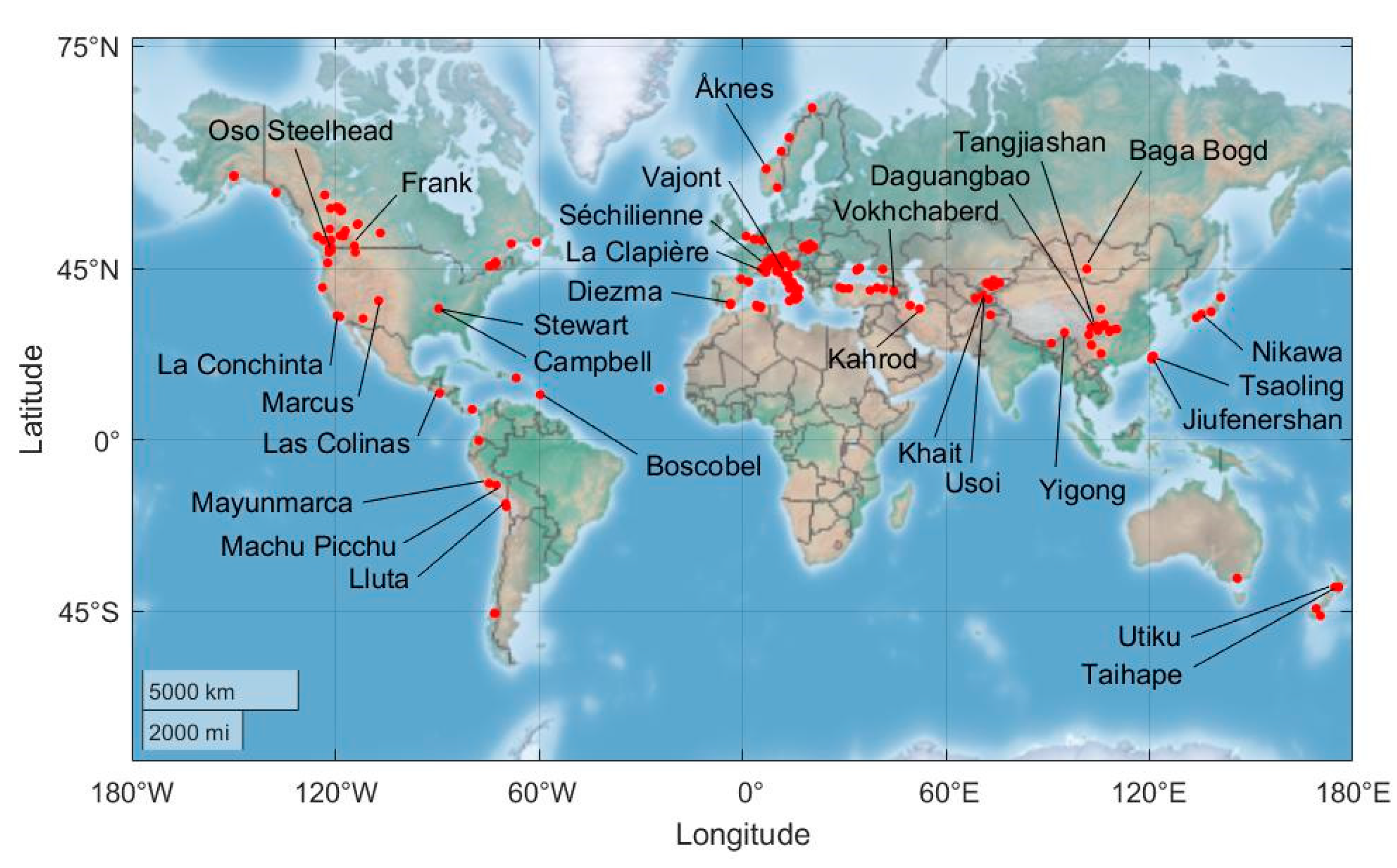
No.	Date	Landslide	C.	Latitude	Longitude	Trigger
001.00	2001-03-18	Diezma	ES	37°18′34.00″ N	003°22′08.70″ W	rain
002.00	1949-07-10	Khait	TJ	39°11′27.40″ N	070°55′41.20″ E	Khait EQ
003.01	paleo	Leupegem Hill 1	BE	50°49′25.07″ N	003°37′18.62″ E	-
003.02	paleo	Leupegem Hill 2	BE	50°49′33.10″ N	003°37′15.99″ E	-
003.03	paleo	Leupegem Hill 3	BE	50°49′36.13″ N	003°37′10.17″ E	-
003.04	paleo	Rotelenberg Hill 4	BE	50°48′32.35″ N	003°34′50.33″ E	-
003.05	paleo	Rotelenberg Hill 5	BE	50°48′37.41″ N	003°34′36.52″ E	-
003.06	paleo	Rotelenberg Hill 6	BE	50°48′43.61″ N	003°34′36.17″ E	-
003.07	paleo	Rotelenberg Hill 7	BE	50°48′45.25″ N	003°34′44.67″ E	-
003.08	paleo	Rotelenberg Hill 8	BE	50°48′48.53″ N	003°34′52.19″ E	-
003.09	paleo	Rotelenberg Hill 9	BE	50°48′47.08″ N	003°35′00.05″ E	-
003.10	paleo	Rotelenberg Hill 10	BE	50°48′45.23″ N	003°35′09.95″ E	-
003.11	paleo	Rotelenberg Hill 11	BE	50°48′43.86″ N	003°35′17.67″ E	-
003.12	paleo	Rotelenberg Hill 12	BE	50°48′48.64″ N	003°35′25.54″ E	-
003.13	paleo	Rotelenberg Hill 13	BE	50°48′53.55″ N	003°35′27.93″ E	-
004.00	?	Büyükçekmece	TR	41°00′34.67″ N	028°37′02.45″ E	overload
005.01	2008-05-12	Chengxi	CN	31°49′33.01″ N	104°26′57.36″ E	Sichuan EQ
005.02	2008-05-12	Xinbei Middle-School	CN	31°49′46.43″ N	104°27′36.25″ E	Sichuan EQ
005.03	2008-05-12	Tangjiashan	CN	31°50′25.30″ N	104°25′59.14″ E	Sichuan EQ
005.04	2008-05-12	Daguangbao	CN	31°38′30.91″ N	104°06′50.34″ E	Sichuan EQ
006.00	?	Lushan Hot Spring	TW	24°01′32.23″ N	121°11′02.25″ E	storm
007.01	1969	Ain El Hammam	DZ	36°34′15.18″ N	004°18′12.23″ E	-
007.02	1970	Tigzirt City	DZ	36°53′10.39″ N	004°08′09.57″ E	-
007.03	2009	Tigzirt Port	DZ	36°53′21.72″ N	004°07′21.78″ E	-
007.04	1952	Azazga	DZ	36°45′21.10″ N	004°23′19.55″ E	-
008.00	2014-03-22	Oso-Steelhead	US	48°17′06.57″ N	121°51′03.33″ W	rain
009.01	1811-12-16	Stewart	US	36°08′32.29″ N	089°31′43.01″ W	New Madrid EQ (#1)
009.02	1811-12-16	Campbell	US	36°04′10.18″ N	089°29′48.84″ W	New Madrid EQ (#1)
010.00	1981-03	Avignonet	FR	44°56′45.29″ N	005°40′47.37″ E	-
011.00	paleo	Braemore	NZ	39°41′29.60″ S	174°39′18.97″ E	-
012.00	2001-01-13	Las Colinas	SV	13°39′46.27″ N	089°17′11.17″ W	El Salvador EQ
013.00	1994-01-08	La Salle en Beaumont	FR	44°52′01.15″ N	005°51′55.74″ E	-
014.00	1978	Harmalière	FR	44°56′07.42″ N	005°40′13.33″ E	-
015.00	1980-11-23	Calitri	IT	40°53′54.88″ N	015°26′09.31″ E	Irpinia EQ
016.01	1999-09-20	Tsaoling	TW	23°35′06.14″ N	120°40′40.83″ E	Chi Chi EQ
016.02	1999-09-20	Jiufenershan	TW	23°57′27.80″ N	120°50′33.79″ E	Chi Chi EQ
016.03	1999-09-20	Hungcaiping	TW	23°57′23.82″ N	120°48′56.63″ E	Chi Chi EQ
017.00	2009-08-09	Shiaolin	TW	23°09′54.85″ N	120°40′00.84″ E	typhoon
018.01	?	Lesachriegel	AT	46°59′17.01″ N	012°40′58.39″ E	-
018.02	?	Gradenbach	AT	46°59′54.02″ N	012°51′00.36″ E	-
019.00	1903-04-29	Frank	CA	49°34′56.75″ N	114°24′31.93″ W	-
020.01	1964-03-28	Potter Hill	US	61°05′23.00″ N	149°50′44.50″ W	Alaska EQ
020.02	1964-03-28	Bluff Road	US	61°14′01.77″ N	149°49′30.78″ W	Alaska EQ
020.03	1964-03-28	Turnagain Heights	US	61°11′56.42″ N	149°57′43.95″ W	Alaska EQ
020.04	1964-03-28	Point Campbell	US	61°08′28.76″ N	150°00′51.40″ W	Alaska EQ
020.05	1964-03-28	Point Woronzof	US	61°12′09.34″ N	150°00′33.05″ W	Alaska EQ
020.06	1964-03-28	L Street	US	61°12′57.46″ N	149°54′31.52″ W	Alaska EQ
020.07	1964-03-28	4th Avenue	US	61°13′11.81″ N	149°53′05.80″ W	Alaska EQ
020.08	1964-03-28	Government Hill	US	61°13′39.83″ N	149°52′23.76″ W	Alaska EQ
020.09	1964-03-28	Native Hospital	US	61°13′16.85″ N	149°52′08.26″ W	Alaska EQ
021.00	1994-01-17	Calabasas	US	34°07′34.43″ N	118°38′58.68″ W	Northridge EQ
022.00	1999-08-17	Degirmendere	TR	40°43′19.56″ N	029°46′56.39″ E	Izmit EQ
023.01	?	Vaculov-Sedlo	CZ	49°23′03.61″ N	018°04′47.13″ E	-
023.02	?	Kobylska	CZ	49°23′08.18″ N	018°12′35.24″ E	-
023.03	?	Kopce	CZ	49°13′20.54″ N	018°02′25.59″ E	-
024.00	1980-05-18	Mt. Saint Helens	US	46°11′57.51″ N	122°11′21.29″ W	volcanism
025.00	paleo	Lluta	CL	18°24′01.65″ S	069°46′27.54″ W	-
026.00	postglacial	Columbia Mountain	US	48°20′18.79″ N	114°07′12.57″ W	deglaciation
027.00	1990-06	Eureka River	CA	56°25′44.79″ N	119°24′05.27″ W	undercutting
028.00	1939-04	Montagneuse River	CA	56°17′24.60″ N	118°52′22.64″ W	-
029.00	1959-05-19	Dunvegan	CA	55°54′28.33″ N	118°37′36.10″ W	-
030.01	2007-05-05	Fox Creek East	CA	55°51′23.82″ N	118°03′25.25″ W	rain
030.02	2007-05-05	Fox Creek West	CA	55°51′32.65″ N	118°04′08.23″ W	rain
031.01	1897	CN50.9	CA	50°42′16.63″ N	121°17′40.51″ W	undercutting
031.02	1886	Goddart	CA	50°41′14.78″ N	121°17′43.30″ W	undercutting
032.00	1883-10-12	Beaver Creek	CA	51°58′56.23″ N	106°43′16.36″ W	-
033.01	?	Mt. Cefalone	IT	42°14′31.49″ N	013°25′13.51″ E	-
033.02	?	Cima della Fossa	IT	41°54′06.97″ N	014°01′32.86″ E	-
033.03	?	Villavallelonga	IT	41°52′03.37″ N	013°39′09.01″ E	-
033.04	1915-01-13	Casali d’Aschi	IT	41°58′01.77″ N	013°40′56.76″ E	Avezzano EQ
033.05	1915-01-13	Gioia dei Marsi	IT	41°57′11.31″ N	013°42′27.76″ E	Avezzano EQ
033.06	1703-01-14	Mt. Alvagnano	IT	42°40′19.15″ N	013°08′40.50″ E	Norcia EQ
033.07	?	Fiamignano	IT	42°16′28.61″ N	013°07′19.02″ E	-
033.08	?	Pescasseroli	IT	41°48′52.62″ N	013°46′21.58″ E	-
034.00	1780	Campo Vallemaggia	CH	46°17′29.96″ N	008°29′36.88″ E	-
035.01	?	Longobardi	IT	39°12′41.17″ N	016°04′19.73″ E	-
035.02	1982-12-13	Ancona	IT	43°36′05.58″ N	013°28′41.16″ E	-
036.00	1984-04	La Clapière	FR	44°15′08.16″ N	006°56′29.22″ E	-
037.00	2006-03-21	Laalam	DZ	36°34′50.09″ N	005°27′24.74″ E	Kherrata EQ
038.00	1806-09-02	Goldau	CH	47°04′36.94″ N	008°33′40.84″ E	rain
039.01	1980	Cerentino	CH	46°18′23.34″ N	008°32′20.52″ E	-
039.02	1834	Peccia	CH	46°24′56.52″ N	008°40′29.50″ E	-
039.03	1846	Val Canaria	CH	46°33′25.52″ N	008°38′49.57″ E	-
039.04	1896-10	Val Colla	CH	46°05′15.13″ N	009°01′08.71″ E	-
040.01	1755-11-01	Güevéjar I	ES	37°15′37.99″ N	003°35′15.10″ W	Lisbon EQ
040.02	1884-12-25	Güevéjar II	ES	37°15′37.99″ N	003°35′15.10″ W	Arenas del Rey EQ
041.00	1683	Montelparo	IT	43°01′11.75″ N	013°32′31.04″ E	-
042.00	1933-10	Sesa	IT	45°54′01.40″ N	010°20′14.35″ E	rain
043.01	?	Ráztoka	SK	48°50′01.71″ N	019°24′20.03″ E	-
043.02	?	Polská Tomanová	SK	49°12′21.83″ N	019°54′57.46″ E	-
044.00	2002-10-31	Salcito	SK	41°44′17.16″ N	014°31′55.14″ E	Molise EQ
045.01	paleo	Belbek	UA	44°40′15.92″ N	033°42′51.45″ E	EQ (?)
045.02	paleo	Frontovoye	UA	44°42′04.50″ N	033°44′45.30″ E	EQ (?)
045.03	paleo	Kacha 1	UA	44°44′47.93″ N	033°43′47.38″ E	EQ (?)
045.04	paleo	Kacha 2	UA	44°45′44.59″ N	033°43′31.12″ E	EQ (?)
045.05	paleo	Alma	UA	44°51′16.53″ N	033°52′43.01″ E	EQ (?)
045.06	paleo	Vishennoye	UA	45°07′57.59″ N	034°36′59.23″ E	EQ (?)
046.01	1692-09-18	Battice 1	BE	50°39′13.63″ N	005°50′24.10″ E	Verviers EQ
046.02	1692-09-18	Battice 2	BE	50°39′00.46″ N	005°50′32.57″ E	Verviers EQ
046.03	1692-09-18	Battice 3	BE	50°38′52.31″ N	005°50′51.36″ E	Verviers EQ
046.04	1692-09-18	Battice 4	BE	50°38′58.66″ N	005°51′29.41″ E	Verviers EQ
046.05	1692-09-18	Battice 5	BE	50°39′00.28″ N	005°51′59.18″ E	Verviers EQ
046.06	1692-09-18	Battice 6	BE	50°39′06.65″ N	005°52′35.11″ E	Verviers EQ
046.07	1692-09-18	Battice 7	BE	50°39′41.62″ N	005°52′38.99″ E	Verviers EQ
046.08	1692-09-18	Battice 8	BE	50°38′27.28″ N	005°51′09.95″ E	Verviers EQ
046.09	1692-09-18	Battice 9	BE	50°38′37.36″ N	005°51′52.67″ E	Verviers EQ
046.10	1692-09-18	Battice 10	BE	50°38′35.84″ N	005°50′45.61″ E	Verviers EQ
046.11	1692-09-18	Battice 11	BE	50°37′53.96″ N	005°49′40.06″ E	Verviers EQ
046.12	1692-09-18	Battice 12	BE	50°37′45.13″ N	005°49′40.99″ E	Verviers EQ
046.13	1692-09-18	Battice 13 (Manaihan)	BE	50°37′34.66″ N	005°49′40.57″ E	Verviers EQ
047.01	2007-04-21	Acantilada Bay	CL	45°23′49.80″ S	072°53′09.00″ W	Aysén EQ
047.02	2007-04-21	Punta Cola	CL	45°22′46.80″ S	072°59′54.00″ W	Aysén EQ
047.03	2007-04-21	Mentirosa Island	CL	45°24′03.00″ S	072°58′05.40″ W	Aysén EQ
047.04	2007-04-21	Frío Creek	CL	45°23′55.20″ S	072°56′40.20″ W	Aysén EQ
047.05	2007-04-21	Marta River 1	CL	45°20′19.80″ S	073°00′15.60″ W	Aysén EQ
047.06	2007-04-21	Fernández Creek	CL	45°23′25.20″ S	072°54′17.40″ W	Aysén EQ
047.07	2007-04-21	Marta River 2	CL	45°20′56.40″ S	072°58′52.20″ W	Aysén EQ
047.08	2007-04-21	Pescado River	CL	45°25′26.40″ S	073°06′05.40″ W	Aysén EQ
048.00	1987-03-05	Salado	EC	00°11′27.68″ S	077°41′39.36″ W	Ecuador EQ
049.00	1679-06-04	Vokhchaberd	AM	40°09′59.75″ N	044°38′17.21″ E	Armenia EQ
050.00	1881-09-10	Castel Frentano	IT	42°11′55.53″ N	014°21′35.41″ E	Lanciano EQ
051.00	1997-10-11	Mt. Nuria	IT	42°21′44.73″ N	013°00′21.11″ E	-
052.01	1990-06-20	Galdian	IR	36°48′01.95″ N	049°25′37.05″ E	Manjil-Rudbar EQ
052.02	1990-06-20	Fatalak	IR	36°50′20.41″ N	049°29′13.48″ E	Manjil-Rudbar EQ
053.00	1963-10-09	Vajont	IT	46°15′27.65″ N	012°20′25.93″ E	rain, GW, bedding
054.00	2003-09-10	Tsaitichhu	BT	27°25′52.19″ N	091°06′40.49″ E	-
055.00	2007-03-01	S. Giovanni	IT	38°16′11.31″ N	015°47′54.28″ E	tunneling
056.00	1950	Rasdeglia	IT	46°27′29.72″ N	009°19′07.28″ E	-
057.00	1992-08-19	Suusamyr	KG	42°12′29.82″ N	073°36′33.08″ E	Suusamyr EQ
058.01	paleo	Kokomeren	KG	41°55′35.84″ N	074°13′35.99″ E	EQ (?)
058.02	1885	Aksu	KG	42°32′33.01″ N	073°59′21.27″ E	Belovodsk EQ (?)
058.03	paleo	Beshkiol	KG	41°25′00.00″ N	074°30′00.00″ E	EQ (?)
058.04	paleo	Karakudjur	KG	41°57′43.72″ N	075°53′09.05″ E	EQ (?)
058.05	1946	Sarychelek	KG	41°52′00.00″ N	072°00′00.00″ E	Chatkal EQ (?)
058.06	paleo	Kugart	KG	41°10′00.00″ N	073°20′60.00″ E	EQ (?)
059.00	?	Rosone	IT	45°26′17.72″ N	007°23′58.78″ E	rain
060.00	2000-04-09	Yigong	CN	30°13′46.30″ N	094°59′28.88″ E	-
061.00	1911-02-18	Usoi	TJ	38°18′21.64″ N	072°36′46.40″ E	Sarez EQ
062.01	1989-01-22	Okuli	TJ	38°29′10.43″ N	068°37′41.70″ E	Gissar EQ
062.02	1989-01-22	May 1	TJ	38°29′15.91″ N	068°37′21.13″ E	Gissar EQ
062.03	1989-01-22	Firma	TJ	38°29′23.60″ N	068°38′19.45″ E	Gissar EQ
062.04	1989-01-22	Sharara	TJ	38°29′17.39″ N	068°38′51.46″ E	Gissar EQ
063.00	1984	Klasgarten	AT	46°57′08.59″ N	010°45′02.24″ E	-
064.00	1975	Niedergallmigg	AT	47°06′04.31″ N	010°36′30.03″ E	-
065.01	1992	Huayuanyangjichang	CN	30°44′57.32″ N	108°25′43.70″ E	GW
065.02	1996	Jinjinzi	CN	30°33′39.48″ N	108°18′17.38″ E	GW
065.03	1999	Yangjiaba	CN	30°26′05.48″ N	108°14′10.50″ E	GW
066.00	postglacial	Atemkopf	AT	46°56′34.29″ N	010°43′19.17″ E	-
067.00	2002-10	La Mania	IT	46°27′24.06″ N	012°43′41.15″ E	-
068.00	1960	Beauregard	IT	45°37′09.03″ N	007°02′36.21″ E	-
069.00	1965-01-09	Hope	CA	49°18′21.72″ N	121°14′22.42″ W	EQ (?)
070.00	?	Anlesi	CN	30°49′45.44″ N	108°20′38.63″ E	rain
071.01	1914-05-30	Cà di Malta	IT	44°17′26.61″ N	011°07′14.63″ E	-
071.02	1934-03-06	Rocca Pitigliana	IT	44°13′56.49″ N	011°00′11.74″ E	-
072.00	1957-07-02	Kahrod	IR	36°03′59.80″ N	052°14′36.17″ E	Mazandaran EQ
073.00	2008-09	Cerca del Cielo	US	18°02′22.22″ N	066°40′28.98″ W	rain
074.00	?	Kutlugün	TR	40°56′31.61″ N	039°43′58.04″ E	-
075.00	1987-07-28	Val Pola	IT	46°22′42.87″ N	010°20′11.95″ E	rain
076.01	?	Varco d’Izzo	IT	40°38′45.97″ N	015°51′40.67″ E	-
076.02	?	Costa della Gaveta	IT	40°38′40.44″ N	015°51′07.42″ E	-
077.00	1979-08-08	Abbotsford	NZ	45°53′37.02″ S	170°26′16.35″ E	mining
078.00	17th cent.	Tortum	TT	40°39′56.10″ N	041°38′31.18″ E	EQ (?)
079.00	18th cent.	Slumgullion	US	37°59′36.97″ N	107°15′11.29″ W	rain
080.00	1999-05-13	Rufi	CH	47°11′15.97″ N	009°04′46.13″ E	rain
081.00	2007	Zhujiadian	CN	31°02′48.86″ N	110°23′57.86″ E	GW
082.00	1982	Minor Creek	US	40°57′57.27″ N	123°49′59.74″ W	rain
083.00	2005-03-17	Kuzulu	TR	40°20′50.13″ N	037°39′16.20″ E	snowmelt
084.00	1995	Huangtupo	CN	31°02′34.17″ N	110°23′07.89″ E	GW
085.00	1998	Fosso Spineto	IT	40°37′38.66″ N	016°17′28.67″ E	undercutting
086.00	500000 BP	Marcus	US	33°40′47.72″ N	111°47′50.06″ W	-
087.00	2003-11-09	Afternoon Creek	US	48°41′33.94″ N	121°14′23.26″ W	rain
088.00	2009-04-26	Valgrisenche	IT	45°41′05.20″ N	007°07′12.24″ E	rain
089.00	?	Aka-Kuzure	JP	35°21′28.03″ N	138°12′26.26″ E	-
090.00	?	Ivancich	IT	43°04′00.00″ N	012°37′30.00″ E	-
091.00	1999-11-12	Bakacak	TR	40°45′19.23″ N	031°22′18.69″ E	Düzce EQ
092.00	postglacial	Triesenberg	LI	47°07′06.22″ N	009°32′54.51″ E	deglaciation
093.00	1783-02-06	Scilla	IT	38°14′53.00″ N	015°42′05.84″ E	Calabria EQ (#2)
094.00	1972	San Donato	IT	40°23′31.15″ N	016°33′54.20″ E	-
095.00	?	La Salsa	IT	40°31′09.71″ N	016°32′50.78″ E	-
096.00	1996	Grohovo	HR	45°21′58.08″ N	014°26′53.11″ E	-
097.00	35000 BP	Uspenskoye	RU	44°53′14.01″ N	041°25′29.77″ E	EQ (?)
098.00	1995-01-16	Nikawa	JP	34°46′23.83″ N	135°20′29.40″ E	Kobe EQ
099.00	paleo	Dúdar	ES	37°11′39.28″ N	003°29′19.66″ W	EQ (?)
100.01	?	Machu Picchu A	PE	13°09′58.60″ S	072°32′26.91″ W	GW, faults
100.02	?	Machu Picchu B	PE	13°09′48.07″ S	072°32′41.83″ W	GW, faults
101.01	2002	Keillor Road	CA	53°30′41.08″ N	113°32′28.92″ W	GW
101.02	1999-10-23	Whitemud Road	CA	53°28′56.19″ N	113°35′17.61″ W	GW
102.00	1627-07-30	Vasto	IT	42°06′16.33″ N	014°42′50.53″ E	Gargano EQ (?)
103.00	1963	Kostanjek	HR	45°49′15.46″ N	015°51′22.44″ E	GW, mining
104.00	1997-07	Mt. Munday	HR	51°20′46.26″ N	125°14′29.02″ W	-
105.00	2010-08-06	Mt. Meager	HR	50°37′27.17″ N	123°30′05.53″ W	volcanism
106.00	10000 BP	Downie	HR	51°30′17.38″ N	118°32′06.37″ W	deglaciation
107.00	2005-01-10	La Conchita	US	34°21′54.51″ N	119°26′40.69″ W	rain
108.00	postglacial	Séchilienne	FR	45°03′49.44″ N	005°48′16.13″ E	-
109.00	2004	Ogoto	JP	?	?	GW
110.00	2003	Kuchi-Otani	JP	?	?	typhoon
111.00	1854-12-23	Zentoku	JP	33°53′07.14″ N	133°50′19.94″ E	Tokai EQ (?)
112.00	2003-05-26	Tsukidate	JP	38°43′41.19″ N	141°00′35.41″ E	Sanriku-Minami EQ
113.01	1997-01	Slesse Park	CA	49°05′05.87″ N	121°48′27.42″ W	rain, logging
113.02	1973-05-26	Attachie	CA	56°12′13.84″ N	121°27′19.17″ W	rain
114.00	1963-09-03	Lesueur	CA	53°36′05.81″ N	113°18′41.57″ W	mining
115.00	1933-07	Brazeau	CA	52°23′21.12″ N	117°04′19.41″ W	-
116.00	1990-06-17	Saddle River	CA	55°47′12.20″ N	118°26′20.37″ W	rain
117.00	2010-01	Cenes de la Vega	ES	37°10′24.38″ N	003°32′01.50″ W	rain, pipe leak
118.00	1993-12-29	Acquara-Vadoncello	IT	40°44′03.30″ N	015°12′42.45″ E	-
119.00	1901-10-01	Boscobel	BB	13°16′27.13″ N	059°34′19.83″ W	-
120.00	paleo	Mt. Nuovo	IT	40°44′08.83″ N	013°53′17.08″ E	volcanism
121.00	140000 BP	Baga Bogd	MN	44°57′37.88″ N	101°32′23.34″ E	deglaciation
122.00	1974-04-25	Mayunmarca	PE	12°39′12.37″ S	074°41′43.58″ W	-
123.00	1612	Corniglio	IT	44°28′00.76″ N	010°04′40.82″ E	-
124.00	?	Vallcebre	ES	42°12′21.23″ N	001°49′59.40″ E	-
125.00	10000 BP	Corvara	IT	46°32′19.74″ N	011°54′13.37″ E	-
126.00	1786-06-01	Dadu River	CN	29°37′52.69″ N	102°09′28.84″ E	Kangding EQ
127.00	10000 BP	Fogo	CV	14°57′06.61″ N	024°21′32.88″ W	volcanism
128.00	1906	Petacciato	IT	42°01′07.49″ N	014°52′39.16″ E	-
129.01	20000 BP	El Petruso	ES	42°48′03.45″ N	000°24′33.85″ W	rain
129.02	20000 BP	Sextas	ES	42°46′12.79″ N	000°22′31.28″ W	rain
129.03	20000 BP	La Selva	ES	42°45′43.54″ N	000°21′10.30″ W	rain
130.00	1996	Halden Creek	CA	58°20′02.94″ N	123°07′45.52″ W	clay
131.00	10000 BP	Åknes	NO	62°10′37.29″ N	006°59′47.45″ E	-
132.00	10000 BP	Kykula	SK	49°26′32.86″ N	018°57′52.44″ E	-
133.00	paleo	Latagualla	CL	19°15′25.20″ S	069°35′42.00″ W	EQ (?)
134.00	1920-12-16	Huihuichuan	CN	35°57′07.79″ N	105°40′07.55″ E	Gansu EQ
135.00	1980	Amloke Nakka	PK	34°34′25.76″ N	073°08′40.24″ E	clay
136.00	1960-10	Tessina	IT	46°11′21.78″ N	012°24′08.15″ E	-
137.00	paleo	Krynica	PL	49°25′01.78″ N	020°57′38.80″ E	deglaciation
138.00	paleo	Collinabos	BE	50°46′11.40″ N	003°34′34.26″ E	loess
139.00	2002-09-06	Cerda	IT	37°56′03.10″ N	013°50′09.54″ E	Cerda EQ
140.00	2011-09-16	Shibangou	CN	32°14′27.00″ N	106°44′45.00″ E	rain
141.00	1996-04-28	Quesnel Forks	CA	52°39′36.09″ N	121°40′12.02″ W	rain
142.00	?	Riou-Bourdoux Valley	FR	44°25′06.29″ N	006°37′20.21″ E	rain
143.00	2000-11-18	Slano Blato	SI	45°54′55.45″ N	013°51′49.12″ E	rain
144.00	1958-07-10	Lituya Bay	US	58°40′53.44″ N	137°29′11.39″ W	Alaska EQ
145.00	1976-05-06	Mt. Boscatz	IT	46°17′19.52″ N	013°04′37.20″ E	Friuli EQ
146.00	1949	Kualiangzi	CN	30°39′01.00″ N	104°53′40.00″ E	rain
147.00	6th cent.	Ropice	CZ	49°36′18.57″ N	018°35′08.10″ E	-
148.00	1982	La Valette	FR	44°24′40.11″ N	006°38′52.84″ E	rain, flysch
149.00	postglacial	Heather Hill	CA	51°26′52.08″ N	117°28′24.24″ W	deglaciation
150.00	2008-11-23	Gongjiafang	CH	31°03′57.62″ N	109°55′11.88″ E	GW
151.00	paleo	Utiku	NZ	39°44′51.09″ S	175°50′16.88″ E	-
152.00	paleo	Taihape	NZ	39°40′56.56″ S	175°47′30.16″ E	-
153.01	paleo	Stromboli	IT	38°47′46.85″ N	015°12′27.06″ E	volcanism
153.02	paleo	La Fossa	IT	38°24′39.37″ N	014°58′02.48″ E	volcanism
154.00	1909-11	East Lirio	PA	09°02′21.69″ N	079°39′02.93″ W	excavation work
155.01	2010-11	Cischele	IT	45°42′42.50″ N	011°13′24.67″ E	-
155.02	?	Ochojno	PL	49°57′39.36″ N	019°57′15.56″ E	-
156.00	postglacial	Gammajunni 3	NO	69°28′48.90″ N	020°33′39.86″ E	-
157.00	postglacial	La Frasse	CH	46°21′31.21″ N	007°02′10.04″ E	-
158.00	1953-01-31	Miramar	UK	51°22′22.79″ N	001°09′17.08″ E	clay
159.00	?	Mahouane Dam	DZ	36°17′24.02″ N	005°21′24.67″ E	clay
160.00	paleo	Pianello	IT	41°14′48.93″ N	015°20′25.04″ E	clay
161.00	2011	St. Maria Maddalena	IT	44°13′05.72″ N	011°11′37.98″ E	tunneling
162.00	?	Zhaoshuling	CN	31°02′38.04″ N	110°20′46.82″ E	GW
163.00	?	Dúrcal	ES	36°55′57.60″ N	003°31′42.36″ W	-
164.00	1935	Aggenalm	DE	47°40′00.28″ N	012°03′28.04″ E	-
165.00	?	Huangshipan	CN	31°54′16.57″ N	106°36′53.68″ E	-
166.00	postglacial	Lake Wanaka	NZ	44°22′13.00″ S	169°11′43.61″ E	EQ (?)
167.00	2015-02-02	Mofjellbekken	NO	59°28′10.11″ N	010°18′02.55″ E	clay
168.00	?	Badu	CN	24°42′36.27″ N	105°47′56.88″ E	excavation work
169.01	paleo	Number 1	CN	26°57′25.06″ N	102°57′54.94″ E	-
169.02	paleo	Number 2	CN	27°00′10.31″ N	102°52′53.13″ E	-
170.01	2005-12-10	Saint Barnabé	CA	46°22′48.83″ N	072°49′24.93″ W	clay
170.02	2010-05-10	Saint Jude	CA	45°48′16.72″ N	072°57′49.13″ W	clay
170.03	1994-04-21	Sainte Monique	CA	46°10′41.46″ N	072°33′05.56″ W	clay
171.00	1970	Bird	NZ	39°37′54.07″ S	175°49′38.10″ E	-
172.00	2013-12-03	Montescaglioso	IT	40°32′31.06″ N	016°39′10.96″ E	-
173.00	19th cent.	Spriana	IT	46°12′41.31″ N	009°52′30.02″ E	-
174.00	?	Piscopio I Tunnel	IT	38°47′05.67″ N	016°33′03.52″ E	tunneling
175.00	?	La Saxe	IT	45°49′02.33″ N	006°58′13.17″ E	-
176.00	?	Erguxi	CN	31°35′59.57″ N	102°49′06.14″ E	-
177.01	1955-12-07	Hawkesbury	CA	45°34′49.52″ N	074°32′47.16″ W	blast (?)
177.02	1962-05-23	Toulnustouc	CA	49°57′47.64″ N	068°08′42.84″ W	blast (?)
177.03	1996-06-20	Finneidfjord	NO	66°10′55.96″ N	013°47′44.52″ E	blast (?)
177.04	2009-03-13	Kattmarka	NO	64°28′26.16″ N	011°26′06.42″ E	blast (?)
177.05	2009-08-01	La Romaine	CA	50°13′24.23″ N	060°40′14.07″ W	blast (?)
178.01	1960	Bumper	AU	37°40′52.09″ S	145°53′55.81″ E	rain
178.02	1960	Siphon Gully	AU	37°41′10.59″ S	145°54′11.54″ E	rain

References

Bird, J.F.; Bommer, J.J. Earthquake losses due to ground failure. Eng. Geol. 2004, 75, 147–179. [Google Scholar] [CrossRef]
Froude, M.J.; Petley, D.N. Global fatal landslide occurrence from 2004 to 2016. Nat. Hazards Earth Syst. 2018, 18, 2161–2181. [Google Scholar] [CrossRef] [Green Version]
Ciurleo, M.; Mandaglio, M.C.; Moraci, N. Landslide susceptibility assessment by TRIGRS in a frequently affected shallow instability area. Landslides 2019, 16, 175–188. [Google Scholar] [CrossRef]
USGS. Landslide Types and Processes. United States Geological Survey Fact Sheet 2004, 3072, 4. Available online: https://pubs.usgs.gov/fs/2004/3072/pdf/fs2004-3072.pdf (accessed on 25 October 2019).
Lott, N.; McCown, S.; Graumann, A.; Ross, T.; Lackey, M. Hurricane Mitch 1999—The Deadliest Atlantic Hurricane since 1780; National Climatic Data Center of the National Oceanic and Atmospheric Administration: Asheville, NC, USA, 1999. Available online: ftp://ftp.ncdc.noaa.gov/pub/data/extremeevents/specialreports/Hurricane-Mitch-1998.pdf (accessed on 8 October 2019).
Yin, Y.P.; Wang, F.W.; Sun, P. Landslide hazards triggered by the 2008 Wenchuan earthquake, Sichuan, China. Landslides 2009, 6/2, 139–151. [Google Scholar] [CrossRef]
Harp, E.L.; Jibson, R.W. Inventory of landslides triggered by the 1994 Northridge, California earthquake. United States Geol. Surv. Open File Rep. 1995, 95, 17. Available online: https://geo-nsdi.er.usgs.gov/metadata/open-file/95-213/ (accessed on 20 May 2020).
Harp, E.L.; Jibson, R.L. Landslides triggered by the 1994 Northridge, California earthquake. Bull. Seismol. Soc. Am. 1996, 86, S319–S332. [Google Scholar]
Keefer, D.K. Landslides caused by earthquakes. Bull. Geol. Soc. Am. 1984, 9, 406–421. [Google Scholar] [CrossRef]
Prestininzi, A.; Romeo, R. Earthquake-induced ground failures in Italy. Eng. Geol. 2000, 58, 387–397. [Google Scholar] [CrossRef]
Rodríguez, C.E.; Bommer, J.J.; Chandler, R.J. Earthquake-induced landslides: 1980–1997. Soil Dyn. Earthq. Eng. 1999, 18, 325–346. [Google Scholar] [CrossRef]
Tanyaş, H.; Van Westen, C.J.; Allstadt, K.E.; Nowicki Jessee, M.A.; Görüm, T.; Jibson, R.W.; Godt, J.W.; Sato, H.P.; Schmitt, R.G.; Marc, O.; et al. Presentation and Analysis of a Worldwide Database of Earthquake-Induced Landslide Inventories. J. Geophys. Res. Earth Surf. 2017, 122, 1991–2015. [Google Scholar] [CrossRef] [Green Version]
Cardinali, M.; Ardizzone, F.; Galli, M.; Guzzetti, F.; Reichenbach, P. Landslides triggered by rapid snow melting: The December 1996—January 1997 event in Central Italy. In Proceedings of the 1st Plinius Conference, Maratea, Italy, 14–16 October 1999; Claps, P., Siccardi, F., Eds.; Bios Publisher: Cosenza, Italy, 2000; pp. 439–448. [Google Scholar]
Schlögel, R.; Torgoev, I.; De Marneffe, C.; Havenith, H.B. Evidence of a changing size–frequency distribution of landslides in the Kyrgyz Tien Shan, Central Asia. Earth Surf. Proc. Land. 2011, 36/12, 1658–1669. [Google Scholar] [CrossRef]
Bucknam, R.C.; Coe, J.A.; Chavarria, M.M.; Godt, J.W.; Tarr, A.C.; Bradley, L.A.; Rafferty, S.; Hancock, D.; Dart, R.L.; Johnson, M.L. Landslides Triggered by Hurricane Mitch in Guatemala—Inventory and Discussion. United States Geol. Surv. Open File Rep. 2001, 443, 40. Available online: https://www.sciencebase.gov/catalog/item/4f4e4b1be4b07f02db6a91b2 (accessed on 20 May 2020). [CrossRef]
Malamud, B.D.; Turcotte, D.L.; Guzzetti, F.; Reichenbach, P. Landslide inventories and their statistical properties. Earth Surf. Proc. Landf. 2004, 29, 687–711. [Google Scholar] [CrossRef]
Brunetti, M.T.; Guzzetti, F.; Rossi, M. Probability distributions of landslide volumes. Nonlinear Process. Geophys. 2009, 16, 179–188. [Google Scholar] [CrossRef]
Guzzetti, F.; Malamud, B.D.; Turcotte, D.L.; Reichenbach, P. Power-law correlations of landslide areas in central Italy. Earth Planet. Sci. Lett. 2002, 195, 169–183. [Google Scholar] [CrossRef]
Guzzetti, F.; Ardizzone, F.; Cardinali, M.; Galli, M.; Reichenbach, P.; Rossi, M. Distribution of landslides in the Upper Tiber River basin, central Italy. Geomorphology 2008, 96, 105–122. [Google Scholar] [CrossRef]
Guzzetti, F.; Mondini, A.C.; Cardinali, M.; Fiorucci, F.; Santangelo, M.; Chang, K.T. Landslide inventory maps: New tools for an old problem. Earth-Sci. Rev. 2012, 112, 42–66. [Google Scholar] [CrossRef] [Green Version]
Korup, O. Distribution of landslides in southwest New Zealand. Landslides 2005, 2, 43–51. [Google Scholar] [CrossRef] [Green Version]
Larsen, I.J.; Montgomery, D.R.; Korup, O. Landslide erosion controlled by hillslope material. Nat. Geosci. 2010, 3, 247–251. [Google Scholar] [CrossRef]
Van Den Eeckhaut, M.; Poesen, J.; Govers, G.; Verstraeten, G.; Demoulin, A. Characteristics of the size distribution of recent and historical landslides in a populated hilly region. Earth Planet. Sci. Lett. 2007, 256, 588–603. [Google Scholar] [CrossRef]
Guzzetti, F.; Ardizzone, F.; Cardinali, M.; Rossi, M.; Valigi, D. Landslide volumes and landslide mobilization rates in Umbria, central Italy. Earth Planet. Sci. Lett. 2009, 279, 222–229. [Google Scholar] [CrossRef]
Havenith, H.B.; Strom, A.; Torgoev, I.; Torgoev, A.; Lamair, L.; Ischuk, A.; Abdrakhmatov, K. Tien Shan Geohazards Database: Earthquakes and landslides. Geomorphology 2015, 249, 16–31. [Google Scholar] [CrossRef]
Hovius, N.; Stark, C.P.; Allen, P.A. Sediment flux from a mountain belt derived by landslide mapping. Geology 1997, 25, 231–234. [Google Scholar] [CrossRef] [Green Version]
Korup, O. Effects of large deep-seated landslides on hillslope morphology, western Southern Alps, New Zealand. J. Geophys. Res. Earth Surf. 2006, 111, 18. [Google Scholar] [CrossRef] [Green Version]
Ten Brink, U.S.; Geist, E.L.; Andrews, B.D. Size distribution of submarine landslides and its implication to tsunami hazard in Puerto Rico. Geophys. Res. Lett. 2006, 33, 4. [Google Scholar] [CrossRef] [Green Version]
Cruden, D.M.; Krahn, J. A Reexamination of the Geology of the Frank Slide. Can. Geotech. J. 1973, 10, 581–591. [Google Scholar] [CrossRef]
Google Earth Pro; Version 7.3.2. Frank Landslide, Canada, 49°35’19.10"N & 114°23’39.35"W, eye altitude 2.53 km, Google 2018, CNES/Airbus 2019, 2019a; Google: Mountain View, CA, USA, 2018.
Domej, G.; Bourdeau, C.; Lenti, L.; Martino, S.; Pluta, K. Mean landslide geometries inferred from a global database of earthquake- and non-earthquake-triggered landslides. Ital. J. Eng. Geol. Environ. 2017, 17, 87–107. [Google Scholar] [CrossRef]
MATLAB; Version 9.7.0 (R2019b); The MathWorks Inc.: Natick, MA, USA, 2019.
IAEG Commission on Landslides. Suggested nomenclature for landslides. Bull. Int. Assoc. Eng. Geol. 1990, 41, 13–16. [Google Scholar] [CrossRef]
Cruden, D.M.; Varnes, D.J. Landslide types and processes. In Landslides: Investigation and Mitigation, 1st ed.; Special Report 247; Turner, A.K., Schuster, R.L., Eds.; National Research Council, Transportation Research Board: Washington, DC, USA, 1996; pp. 36–75. [Google Scholar]
Delgado, J.; Garrido, J.; Lenti, L.; Lopez-Casado, C.; Martino, S.; Sierra, F.J. Unconventional pseudostatic stability analysis of the Diezma landslide (Granada, Spain) based on a high-resolution engineering-geological model. Eng. Geol. 2015, 184, 81–95. [Google Scholar] [CrossRef] [Green Version]
Google Earth Pro; Version 7.3.2. Diezma Landslide, Spain, 37°18’34.00"N & 3°22’8.70"W, eye altitude 2.03 km, Google 2018, Europa Technologies 2018, 2019b; Google: Mountain View, CA, USA, 2018.
Varnes, D.J. Slope movement types and processes. In Landslides—Analysis and Control, 1st ed.; Special Report 176; Schuster, R.L., Krizek, R.J., Eds.; National Research Council, Transportation Research Board: Washington, DC, USA, 1978; pp. 11–33. [Google Scholar]
Stark, C.P.; Guzzetti, F. Landslide rupture and the probability distribution of mobilized debris volumes. J. Geophys. Res. Earth 2009, 114, 16. [Google Scholar] [CrossRef]
Heim, A. Bergsturz und Menschenleben, Beiblatt zur Vierteljahrsschrift der Naturforschenden Gesellschaft in Zürich no. 20; Fretz & Wasmuth: Tübingen, Germany, 1932; p. 218. [Google Scholar]
Domej, G. Seismically Induced Effects and Slope Stability In Urbanized Zones by Numerical Modeling. Ph.D. Thesis, Institut Français des Sciences et Technologies des Transports, de l’Aménagement et des Réseaux & Université Paris–Est, Paris, France, 2018; p. 266. [Google Scholar]
ISO. ISO 3166 Country Codes; International Organization for Standardization: Geneva, Switzerland, 2013; Available online: https://www.iso.org/iso-3166-country-codes.html (accessed on 25 October 2019).

Figure 1. Comparison (identical (a), overlap (b), adjacent (c), and offset (d)) of rupture zones and landslide zones (i.e., entire zones affected by sliding processes, which are mainly dependent on the location of the landslide deposits).

Figure 2. Difference between the entire landslide zone and the rupture zone exemplified by the Frank Landslide, Canada (No. 019.00 in Table A1 in the Appendix A). Zones are drawn after Cruden and Krahn [29] (satellite imagery from Google Earth Pro [30]).

Figure 3. Locations of the 277 landslides included in the database (map from MATLAB [32]).

Figure 4. Description of parameters defining a landslide rupture zone (adapted and further developed from the IAEG Commission on Landslides [33]).

Figure 5. Schematic example of measurement of the parameters defining the rupture zone of the Diezma Landslide, Spain (No. 001.00 in Table A1 in the Appendix A). Cross sections are drawn after Delgado et al. [35] (satellite imagery from Google Earth Pro [36]).

Figure 6. Schematic representation of the statistical approach. Landslides of a particular set are screened for showing a calculated volume (V_equ). Those that also show a variable of correlation (e.g., maximum depth (D), reported slope angle (α_lit), or the ratio of the maximum width and the length along the slope (W/L)) are then used for plots that illustrate the respective correlation. The right part of the figure shows examples of usage of the established correlations.

Figure 7. Examples of volume to parameter correlations for the set “full”. Dimension-related parameters (D (a), H_0E (b), and L (c)) are approximated by a regression; for the shape-related parameter (α_equ (d)), the mean value (μ) is calculated. The shading indicates the symmetric belts of two standard deviations (±1σ) around the mean value (μ); the latter is very similar to the “forced” regression (regression parameters in Table 3).

Figure 8. Examples of volume-to-ratio correlations for the set “full”. For shape-related parameters (i.e., here the ratios; H_0E/L_h (a), d_av5/L (b), w_av5/L (c), and d_av5/w_av5 (d)), the mean values (µ) are calculated. The shadings indicate the symmetric belts of two standard deviations (±1σ) around the mean values (µ).

Figure 9. Comparison of regressions (D (a), H_0E (b), L (c), and W (d)) of the six tested sets and the respective average regression, as shown in Table 6a. The shadings indicate the visually derived zones of maximum overlap.

Figure 10. Schematic representation of ratios of dimension-related parameters. All schematic drawings correspond to the average ratios found by the volume-to-ratio-correlation shown in Table 6c.

Figure 11. Comparison (H_0E/L_h (a), d_av5/L (b), w_av5/L_(h) (c), and d_av5/w_av5 (d)) of mean values of ratios (µ) for the six tested sets and the respective average mean value (µ) of this publication (Table 5 and Table 6c; left subplots) and of the average of the mean values (µ) per set as presented in Domej et al. [31] (Table 7; right subplots).

Table 1. Description of parameters defining a landslide rupture zone (adapted and further developed from the IAEG Commission on Landslides [33]). The last column indicates the type of statistical distribution of values per individual parameter throughout the database.

Parameters	Description	Statistical Distribution
V_equ	calculated volume (= (1/6)·π·L·D·W))	increasing exponential
A	area as reported by literature	increasing exponential
A_h	area projected to the horizontal	increasing exponential
L	length along the slope	increasing exponential
L_h	length projected to the horizontal	increasing exponential
H_max	height between point 0 and the deepest point	increasing exponential
H_0E	height between point 0 and point E	increasing exponential
W	maximum width	increasing exponential
w₀, w₁, w₂, w₃, w_E	widths at points 0 to E	increasing exponential
D	maximum depth	increasing exponential
d₀, d₁, d₂, d₃, (d_E)	depths at points 0 to E	normal (d_E is always 0)
δ₀, δ₁, δ₂, δ₃, δ_E	angles at points 0 to E	normal
cur	curvature of the rupture surface (= δ₀₋δ_E)	normal
α_lit	reported slope angle	normal
α_equ	calculated slope angle (= tan⁻¹(H_0E/L_h))	normal
d_1t, d_2t, d_3t	maximum depths of TCS I to III	(TCS: too few data; argumentation in 2.1.)
γ_1L, γ_2L, γ_3L	left flank angles of TCS I to III
γ_1R, γ_2R, γ_3R	right flank angles of TCS I to III

Table 2. Subsets of the database used for analyses with their respective first and second filters.

Set	Filter 1	Filter 2	Included Cases
1—“full”	-	landslide only	240
2—“SR”	landslides in seismic regions		189
3—“EQt”	earthquake-triggered landslides		95
4—“full-R”	rotational landslides		76
5—“full-T”	translational landslides		79
6—“full-RT”	roto-translational		85

Table 3. Results for the volume-to-parameter correlations for the set “full”. For all dimension and shape-related parameters, the regression parameters (R², RMSE, constant (a) and factor (b) with their 95% confidence intervals; Equation (2)) are given.

V_equ/	Cases		R²	RMSE	Constant (a)	Factor (b)
D	176	double-logarithmic fitting	0.75	0.22	−0.29 (±0.18)	0.29 (±0.02)
d_av5	153		0.75	0.23	−0.65 (±0.20)	0.29 (±0.03)
d_av4	153		0.75	0.23	−0.55 (±0.20)	0.29 (±0.03)
d_av3	153		0.75	0.23	−0.46 (±0.20)	0.30 (±0.03)
d₀	153		d₀ contains 0, not fitted in a log-log
d₁	153		0.73	0.24	−0.41 (±0.21)	0.30 (±0.03)
d₂	153		0.71	0.25	−0.37 (±0.21)	0.29 (±0.03)
d₃	153		0.66	0.30	−0.63 (±0.25)	0.31 (±0.04)
d_E	153		d_E is always 0, not fitted in a log-log
H_0E	176		0.60	0.34	−0.06 (±0.28)	0.32 (±0.04)
H_max	176		0.63	0.32	−0.06 (±0.26)	0.33 (±0.04)
L	176		0.88	0.17	0.32 (±0.14)	0.36 (±0.02)
L_h	176		0.88	0.17	0.27 (±0.14)	0.36 (±0.02)
W	176		0.82	0.21	0.25 (±0.17)	0.36 (±0.02)
w_av5	169		0.80	0.22	0.15 (±0.19)	0.35 (±0.03)
w_av3	169		0.81	0.22	0.23 (±0.18)	0.35 (±0.03)
w₀	169		0.57	0.36	0.02 (±0.30)	0.32 (±0.04)
w₁	169		0.78	0.24	0.23 (±0.19)	0.34 (±0.03)
w₂	169		0.78	0.24	0.25 (±0.20)	0.34 (±0.03)
w₃	169		0.78	0.24	0.21 (±0.20)	0.35 (±0.03)
w_E	169		0.63	0.35	−0.02 (±0.29)	0.36 (±0.04)
δ₀	153	x-semi-logarithmic	0.03	19.21	67.00 (±16.35)	−2.36 (±2.28)
δ₁	153		0.02	13.99	28.32 (±11.90)	−1.41 (±1.66)
δ₂	153		0.00	13.97	17.06 (±11.88)	−0.32 (±1.66)
δ₃	153		0.00	11.58	8.59 (±09.85)	0.32 (±1.38)
δ_E	153		0.00	16.92	0.15 (±14.39)	−0.16 (±2.01)
cur	153		0.01	25.26	66.84 (±21.50)	−2.21 (±3.00)
α_equ	176		0.01	11.71	22.86 (±09.53)	−0.70 (±1.35)
α_lit	84		0.00	13.31	19.96 (±16.23)	−0.01 (±2.32)

Table 4. Results for the volume-to-parameter correlations for the set “full”. For all shape-related parameters, the mean value (µ) with the respective standard deviation (σ) and the sample size per sigma interval is given.

V_equ/	Cases	µ	σ	µ/σ	% in ±1σ	% in ±2σ	% in ±3σ
δ₀	153	50.37	19.41	2.59	66.0%	97.4%	100.0%
δ₁	153	18.42	14.07	1.31	66.7%	96.7%	100.0%
δ₂	153	14.83	13.93	1.06	76.5%	94.1%	98.7%
δ₃	153	10.81	11.55	0.94	82.4%	94.8%	98.7%
δ_E	153	−0.96	16.86	−0.06	73.9%	94.1%	98.0%
cur	153	51.33	25.36	2.02	70.6%	97.4%	99.4%
α_equ	176	17.99	11.71	1.54	71.0%	94.3%	98.9%
α_lit	84	19.90	13.23	1.50	73.8%	97.6%	98.8%

Table 5. Results for volume-to-ratio correlations for the set “full”. For all shape-related parameters (i.e., here the ratios), the mean values (µ) with the respective standard deviations (σ) and the sample sizes per sigma interval are given.

V_equ/	Cases	µ	σ	µ/σ	% in ±1σ	% in ±2σ	% in ±3σ
H_0E/L_h	176	0.35	0.27	1.29	82.4%	94.3%	98.3%
H_max/L_h	176	0.36	0.27	1.34	82.4%	94.9%	98.3%
H_0E/W	176	0.49	0.51	0.96	88.6%	96.0%	97.7%
H_0E/w_av5	169	0.72	0.77	0.93	88.2%	95.9%	97.6%
H_0E/w_av3	169	0.62	0.69	0.90	88.8%	95.3%	98.2%
H_0E/D	176	3.92	3.42	1.15	85.2%	97.7%	98.3%
H_0E/d_av5	153	7.85	5.84	1.34	85.0%	93.5%	97.4%
H_0E/d_av4	153	6.28	4.67	1.34	85.0%	93.5%	97.4%
H_0E/d_av3	153	4.87	3.62	1.35	83.7%	94.8%	97.4%
D/L	176	0.11	0.09	1.31	81.3%	90.3%	99.4%
d_av5/L	153	0.05	0.03	1.46	75.8%	94.1%	99.4%
d_av4/L	153	0.06	0.04	1.45	75.8%	94.1%	99.4%
d_av3/L	153	0.08	0.06	1.45	74.5%	94.1%	99.4%
W/L	176	1.17	1.38	0.85	92.1%	97.2%	97.7%
w_av5/L	169	0.82	0.90	0.91	89.9%	97.0%	98.2%
w_av3/L	169	0.95	1.01	0.95	91.1%	97.0%	98.2%
D/W	176	0.15	0.14	1.02	89.2%	94.3%	97.2%
D/w_av5	169	0.21	0.19	1.10	87.0%	94.7%	97.6%
D/w_av3	169	0.17	0.16	1.07	88.2%	95.3%	98.8%
d_av5/W	153	0.07	0.08	0.89	92.8%	97.4%	97.4%
d_av4/W	153	0.09	0.10	0.89	92.8%	97.4%	97.4%
d_av3/W	153	0.11	0.13	0.89	92.8%	97.4%	98.0%
d_av5/w_av5	146	0.10	0.10	0.92	94.5%	98.6%	98.6%
d_av3/w_av3	146	0.13	0.16	0.84	93.8%	98.6%	98.6%

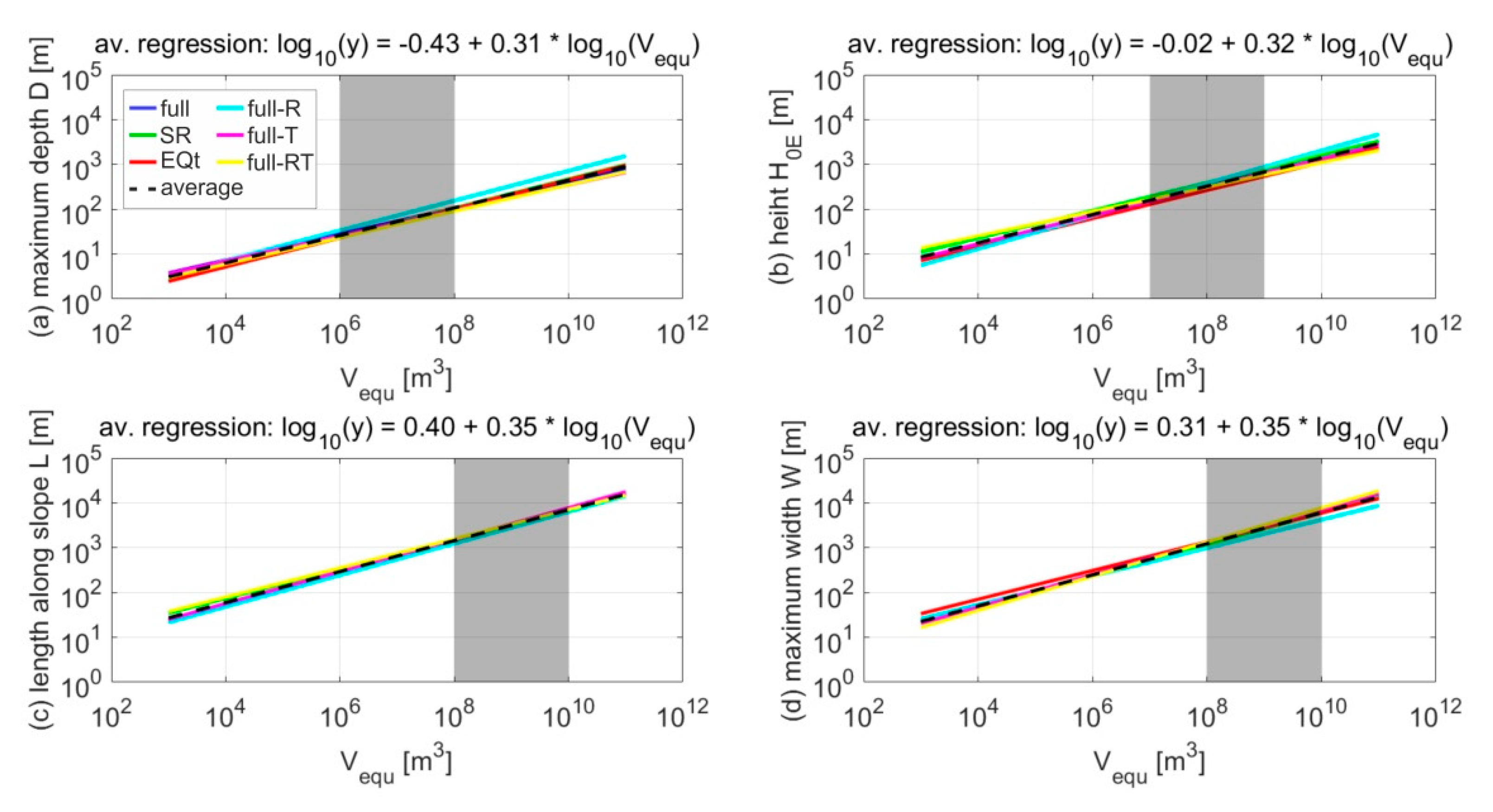
Table 6. Average results for the volume-to-parameter correlations (a, b) and for the volume-to-ratio correlations (c). For all dimension-related parameters (a), the average regression parameters (constant (a) and factor (b); Equation (2)) are given; for all shape-related parameters (b, c), the table shows the average mean values (µ) with the respective average standard deviations (σ). As d₀ contains 0 and d_E is always 0, they are not fitted in a double-logarithmic diagram.

(a) V_equ/	Average Regression Parameters (co. (a) \| fa. (b))	(b) V_equ/	Average Horizontal Reference Line (µ \| σ)	(c) V_equ/	Average Horizontal Reference Line (µ \| σ)
D	−0.43 \| 0.31	δ₀	50.15 \| 19.65	H_0E/L_h	0.35 \| 0.28
d_av5	−0.71 \| 0.30	δ₁	18.65 \| 13.85	H_max/L_h	0.36 \| 0.27
d_av4	−0.61 \| 0.30	δ₂	15.15 \| 14.07	H_0E/W	0.49 \| 0.51
d_av3	−0.52 \| 0.31	δ₃	10.86 \| 11.62	H_0E/w_av5	0.71 \| 0.75
d₀	-	δ_E	-0.27 \| 16.84	H_0E/w_av3	0.61 \| 0.67
d₁	−0.49 \| 0.31	cur	50.42 \| 25.11	H_0E/D	3.99 \| 3.25
d₂	−0.44 \| 0.30	α_equ	18.10 \| 12.01	H_0E/d_av5	7.90 \| 5.82
d₃	−0.69 \| 0.31	α_lit	20.75 \| 12.86	H_0E/d_av4	6.32 \| 4.65
d_E	-			H_0E/d_av3	4.91 \| 3.58
H_0E	−0.02 \| 0.32			D/L	0.10 \| 0.07
H_max	−0.02 \| 0.32			d_av5/L	0.05 \| 0.03
L	0.40 \| 0.35			d_av4/L	0.06 \| 0.04
L_h	0.34 \| 0.35			d_av3/L	0.08 \| 0.05
W	0.31 \| 0.35			W/L	1.22 \| 1.47
w_av5	0.18 \| 0.34			w_av5/L	0.84 \| 0.89
w_av3	0.27 \| 0.34			w_av3/L	0.97 \| 1.00
w₀	0.00 \| 0.32			D/W	0.14 \| 0.12
w₁	0.25 \| 0.34			D/w_av5	0.19 \| 0.16
w₂	0.28 \| 0.34			D/w_av3	0.16 \| 0.14
w₃	0.25 \| 0.34			d_av5/W	0.07 \| 0.07
w_E	0.03 \| 0.35			d_av4/W	0.09 \| 0.09
				d_av3/W	0.11 \| 0.12
				d_av5/w_av5	0.09 \| 0.10
				d_av3/w_av3	0.13 \| 0.14

Table 7. Ratios per volume group as reported in Domej et al. [31]. The value triplets correspond to the ratios per tested set (“full” (^a), “SR” (^b), and “EQt” (^c)).

Ratios in Domej et al. [31]	Group 10³–10⁶ m³	Group 10⁶–10⁹ m³	Group 10⁹–10¹² m³	Average per Set
H_0E/L_h	0.34 ^a 0.38 ^b 0.29 ^c	0.33 ^a 0.35 ^b 0.29 ^c	0.25 ^a 0.32 ^b 0.23 ^c	0.31 ^a 0.35 ^b 0.27 ^c
d_av5/L	0.05 ^a 0.05 ^b 0.05 ^c	0.04 ^a 0.04 ^b 0.03 ^c	0.05 ^a 0.06 ^b 0.06 ^c	0.05 ^a 0.05 ^b 0.05 ^c
w_av5/L_h	0.85 ^a 0.60 ^b 1.48 ^c	0.63 ^a 0.58 ^b 0.80 ^c	0.89 ^a 0.83 ^b 0.91 ^c	0.79 ^a 0.67 ^b 1.06 ^c
d_av5/w_av	0.07 ^a 0.09 ^b 0.04 ^c	0.07 ^a 0.07 ^b 0.04 ^c	0.06 ^a 0.08 ^b 0.07 ^c	0.07 ^a 0.08 ^b 0.05 ^c

© 2020 by the authors. Licensee MDPI, Basel, Switzerland. This article is an open access article distributed under the terms and conditions of the Creative Commons Attribution (CC BY) license (http://creativecommons.org/licenses/by/4.0/).

Share and Cite

MDPI and ACS Style

Domej, G.; Bourdeau, C.; Lenti, L.; Martino, S.; Pluta, K. Shape and Dimension Estimations of Landslide Rupture Zones via Correlations of Characteristic Parameters. Geosciences 2020, 10, 198. https://0-doi-org.brum.beds.ac.uk/10.3390/geosciences10050198

AMA Style

Domej G, Bourdeau C, Lenti L, Martino S, Pluta K. Shape and Dimension Estimations of Landslide Rupture Zones via Correlations of Characteristic Parameters. Geosciences. 2020; 10(5):198. https://0-doi-org.brum.beds.ac.uk/10.3390/geosciences10050198

Chicago/Turabian Style

Domej, Gisela, Céline Bourdeau, Luca Lenti, Salvatore Martino, and Kacper Pluta. 2020. "Shape and Dimension Estimations of Landslide Rupture Zones via Correlations of Characteristic Parameters" Geosciences 10, no. 5: 198. https://0-doi-org.brum.beds.ac.uk/10.3390/geosciences10050198

Note that from the first issue of 2016, this journal uses article numbers instead of page numbers. See further details here.

(a) V_equ/	Average Regression Parameters (co. (a) \| fa. (b))	(b) V_equ/	Average Horizontal Reference Line (µ \| σ)	(c) V_equ/	Average Horizontal Reference Line (µ \| σ)
D	−0.43 \| 0.31	δ₀	50.15 \| 19.65	H_0E/L_h	0.35 \| 0.28
d_av5	−0.71 \| 0.30	δ₁	18.65 \| 13.85	H_max/L_h	0.36 \| 0.27
d_av4	−0.61 \| 0.30	δ₂	15.15 \| 14.07	H_0E/W	0.49 \| 0.51
d_av3	−0.52 \| 0.31	δ₃	10.86 \| 11.62	H_0E/w_av5	0.71 \| 0.75
d₀	-	δ_E	-0.27 \| 16.84	H_0E/w_av3	0.61 \| 0.67
d₁	−0.49 \| 0.31	cur	50.42 \| 25.11	H_0E/D	3.99 \| 3.25
d₂	−0.44 \| 0.30	α_equ	18.10 \| 12.01	H_0E/d_av5	7.90 \| 5.82
d₃	−0.69 \| 0.31	α_lit	20.75 \| 12.86	H_0E/d_av4	6.32 \| 4.65
d_E	-			H_0E/d_av3	4.91 \| 3.58
H_0E	−0.02 \| 0.32			D/L	0.10 \| 0.07
H_max	−0.02 \| 0.32			d_av5/L	0.05 \| 0.03
L	0.40 \| 0.35			d_av4/L	0.06 \| 0.04
L_h	0.34 \| 0.35			d_av3/L	0.08 \| 0.05
W	0.31 \| 0.35			W/L	1.22 \| 1.47
w_av5	0.18 \| 0.34			w_av5/L	0.84 \| 0.89
w_av3	0.27 \| 0.34			w_av3/L	0.97 \| 1.00
w₀	0.00 \| 0.32			D/W	0.14 \| 0.12
w₁	0.25 \| 0.34			D/w_av5	0.19 \| 0.16
w₂	0.28 \| 0.34			D/w_av3	0.16 \| 0.14
w₃	0.25 \| 0.34			d_av5/W	0.07 \| 0.07
w_E	0.03 \| 0.35			d_av4/W	0.09 \| 0.09
				d_av3/W	0.11 \| 0.12
				d_av5/w_av5	0.09 \| 0.10
				d_av3/w_av3	0.13 \| 0.14

Article Menu

Shape and Dimension Estimations of Landslide Rupture Zones via Correlations of Characteristic Parameters

Abstract

1. Introduction

2. Statistical Analyses

2.1. Volume-to-Parameter Correlations

2.2. Volume-to-Ratio Correlations

3. Discussion of Results of All Six Sets

4. Conclusions and Perspectives

Author Contributions

Funding

Data Sources

Conflicts of Interest

Appendix A

References

Share and Cite

Article Metrics

Article Access Statistics

Further Information

Guidelines

MDPI Initiatives

Follow MDPI