Parameterization of a Bayesian Normalized Difference Water Index for Surface Water Detection


1
Facoltà di Ingegneria ed Architettura, Università degli Studi di Enna Kore, 94100 Enna, Italy
2
Dipartimento di Ingegneria, Università degli Studi di Palermo, 90128 Palermo, Italy
*
Author to whom correspondence should be addressed.
Geosciences 2020, 10(7), 260; https://0-doi-org.brum.beds.ac.uk/10.3390/geosciences10070260
Submission received: 18 May 2020
/
Revised: 2 July 2020
/
Accepted: 6 July 2020
/
Published: 7 July 2020
(This article belongs to the Special Issue Recent Advances in Remote Sensing Techniques for Natural Hazard Analysis)
Abstract
:The normalized difference water index (NDWI) has been extensively used for different purposes, such as delineating and mapping surface water bodies and monitoring floods. However, the assessment of this index (based on multispectral remote sensing data) is highly affected by the effects of atmospheric aerosol scattering and built-up land, especially when green and near infrared bands are used. In this study, a modified version of the NDWI was developed to improve precision and reliability in the detection of water reservoirs from satellite images. The proposed equation includes eight different parameters. A Bayesian procedure was implemented for the identification of the optimal set of these parameters. The calculation of the index was based on Sentinel-2 satellite images of spectral bands collected over the 2015–2019 period. The modified NDWI was tested for the identification of small reservoirs in a subbasin of the Belice catchment in Sicily (southern Italy). To assess the effectiveness of the index, a reference image, representing the actual reservoirs in the study area, was used. The results suggested that the use of the proposed methodology for the parameterization of the modified NDWI improves the identification of water reservoirs with surfaces smaller than 0.1 ha.
1. Introduction
The accurate mapping of surface water can provide useful information for water resource, drought, and flood management by supporting water policy definitions and decision-making processes. Remote sensing techniques have shown powerful capabilities to map and monitor surface water [1]. The most frequently used methods are based on reflected solar radiation or active microwave emissions [2]. The former can be divided into single- and multiband methods, where two or more spectral band combinations allow us to highlight the difference between water surfaces and land areas. In particular, near infrared (NIR) radiation is used in single-band techniques because it is highly adsorbed by water, while it is highly reflected by vegetation and dry soil. Low values of reflectance at NIR frequencies are associated not only with the presence of water but also with moist and bare soils. To overcome this issue, the joint use of other frequencies was investigated, and the normalized difference water index (NDWI), together with other water indexes, was defined.
Several NDWI formulations have been proposed in the literature [2,3,4,5]. The index is a single number that is computed as the normalized difference of two or more spectral bands. A suitable threshold value is then established to classify water bodies from other land cover features on the basis of the spectral qualities.
Gao [3] defined the NDWI as the normalized difference between NIR and middle infrared (MIR) bands, and although it was originally developed for vegetation water assessment (see [6] for an application), some studies used it for the identification of open water bodies [7] in desert areas [8]. McFeeters [2] proposed an NDWI using the green (G) and NIR channels of Landsat MSS, while Xu [5] substituted shortwave infrared (SWIR) from Landsat TM to NIR to overcome the errors that affect the NDWIG-NIR derived from the presence of built-up lands, vegetation, and soil. Rogers and Kearney [4] presented an NDWI calculated using the red (R) and SWIR bands of Landsat TM.
The abovementioned NDWI formulations have been widely applied, and their suitability and limitations have been assessed for several applications, using different sensors with respect to those for which they were originally tested. Using Landsat imagery, Rokni et al. [9] compared some NDWI formulations (specifically the NDWIG-NIR and NDWIG-MIR) with other water indexes (normalized difference moisture index, water ratio index, normalized difference vegetation index, and automated water extraction index) for saline lake water extraction, and found that the NDWIG-NIR achieves better results compared to those of other indexes. Liu et al. [10] confirmed that the NDWIG-NIR showed good performance for the analyzed case studies of four large lakes in China, especially if a proper threshold was defined. Nevertheless, studies carried out by Soti et al. [11] and Campos et al. [8] demonstrated that the NDWIG-NIR is less efficient for detecting water bodies in arid areas compared with indexes proposed by Gao [3] and Xu [5]. Ji et al. [1] investigated the influence of soil and vegetation subpixels at a given water fraction on the NDWI threshold. Moreover, for four different satellite sensors (Landsat ETM+, SPOT-5, ASTER, and MODIS), they recommended the NDWIG-SWIR as having a more stable threshold and the least influence from the vegetation component.
The use of the NDWI has not been limited to the detection of water bodies. Recently, Dai et al. [12] proposed a NDWI-based algorithm to improve the reliability of coastline extraction from high- resolution multispectral images. The methodology has been applied to a wide test region (including North Canada, Alaska, Greenland, Iceland, the Scandinavian Peninsula, and the northern area of Russia), providing an accurate mapping of coastline over large areas.
Water body extraction with optical techniques can be improved, as long as shadows (including the shadows of mountains, buildings, clouds, etc.) and noise within the water are reduced or eliminated [13]. The methods usually applied to address these issues are support vector machines (SVMs) and traditional neural networks (NNs). Principal component analysis (PCA), which is able to produce uncorrelated output bands and reduce noise, was also used to enhance NDWI performance in water extraction, e.g., for lake temporal dynamics [9] and for urban areas and mountains [14]. NDWIs have also been tested for delineating flood-prone areas and monitoring flooding [15,16,17,18]. Whereas most of the studies cited above faced the extraction of large and medium water bodies or flooding areas, small reservoirs have been largely neglected in hydrological and water resource research due to their small size, existence in large numbers, and widespread distribution [19]. Nevertheless, they are important for overcoming minor droughts in rural areas [20], for epidemic control [11,21], and for modifying runoff processes entering large downstream reservoirs [22]. In the literature, the extraction of small reservoirs, as for large and medium water bodies, has been performed by water indexes using multispectral [11,20,21,22] or synthetic aperture radar (SAR) data [19,23,24]. Among these studies, only a few address very small reservoirs (<1 ha) [11,21,24].
In this study, to improve the accuracy in extracting small surface water bodies (0.1 ha), a modified version of the NDWI has been proposed by using the four 10-m resolution spectral bands of Sentinel-2 images. A Bayesian procedure has been developed and used to identify the optimal values of the parameters included in the modified formulation. The proposed methodology has been tested for a case study located in Sicily (southern Italy). The use of the modified index is not limited to the detection of surface water features but can be easily extended to other applications, such as the delineation of flooded areas.
The paper is organized as follows. In Section 2, the materials and methods are presented. Specifically, in Section 2.2, the proposed Bayesian approach is described. In Section 2.3, the case study and the dataset are briefly described. The results are presented and discussed in Section 3. In Section 4, the main findings of the study are briefly summarized.
2. Materials and Methods
2.1. The Modified NDWI
The NDWI is a methodology based on the use of remotely sensed digital data and was developed to detect surface water features [2]. As mentioned above, the NDWI uses visible green light and reflected near infrared radiation according to the following equation [25]:
where ρ3 and ρ8 are the top-of-atmosphere (TOA) reflectance of band 3 (green) and band 8 (near infrared) of Sentinel-2, respectively. The NDWI ranges from −1 to 1; typically, the cover type is water when the NDWI > 0 and non-water when the NDWI ≤ 0. Nevertheless, several studies were carried out to identify the optimal NDWI threshold, showing that it may be variable depending on atmospheric conditions, vegetation land cover, the presence of vegetation around water surfaces, and climate [26,27,28].
In most cases, the NDWI is an effective index for the detection of water bodies, even if it tends to be affected by built-up land and cloudiness. When the index is used to produce maps of water bodies, this sensitivity can increase the number of false positives (the identification of a water surface feature when absent).
The NDWI includes spectral bands 3 and 8. To improve the accuracy of the method in extracting surface water bodies, Equation (1) was modified, introducing more spectral bands to enhance water features and eliminate noise components. Thus, the proposed index includes the four 10-m resolution spectral bands of Sentinel-2 images, as follows:
where ρ2, ρ3, ρ4, and ρ8 are the TOA reflectances of band 2 (blue), band 3 (green), band 4 (red), and band 8 (near infrared), respectively, and α, β, γ, δ, ε, η, ϑ, and ζ are parameters with no physical meaning to be calibrated. The proposed index expression maintains the characteristics of the original NDWI formulation, in which the NIR (band 8) is in the numerator and the denominator of the fraction. The NDWI, depending only on band 3 and band 8, lacks effectiveness in distinguishing wet vegetated soil and water. To overcome this issue, in the NDWIm formula, all three visible bands (bands 2, 3, and 4) are included. Indeed, considering the other visible bands in the formulation improves the identification of reservoirs, increasing the efficiency of the index in discriminating water from vegetation.
2.2. The Proposed Parameterization Methodology
As previously mentioned, the calculation of the proposed modified NDWI requires the assessment of eight parameters. Detecting the optimal set of these parameters is essential for reducing the uncertainty related to the extraction of surface water bodies.
A Bayesian procedure was applied to evaluate the optimal set of the parameters in Equation (2). The identification of this set was performed by comparing the locations of reservoirs obtained by applying the proposed formula with those reported on a map of actual reservoirs in the analyzed catchment.
The Bayesian analysis is based on the assessment of a model parameter in terms of probability. Assume that Y = {y1, y2,…, yn} is a vector of n data observations and w = {w1, w2,…,wm} is a vector of m model parameters to be evaluated. According to the Bayesian approach [29], the uncertainty related to a model parameter can be assessed, starting from a prior probability distribution that describes the current state of knowledge about such a parameter before data measurements. The availability of new observations affects the uncertainty linked to parameter estimation; therefore, the probability distribution can be updated accounting for the posterior distribution. Once data have been observed, the Bayesian formulation for the posterior distribution can be applied using the following equation [30,31]:
where and indicate the prior and posterior distributions of parameters, respectively, is the likelihood function of the model, and is a scalar normalization constant that forces the equation to integrate to 1. The likelihood function is the joint probability function of data as a function of parameters and represents the distance between the model predictions and the corresponding data measurements. Assuming that the residual errors are normally distributed and uncorrelated, the normal likelihood function can be used. To assess the validity of this assumption, a posterior diagnostic check of residual errors (e.g., Q–Q plot analysis) needs to be performed. Alternatively, in the case of non-normal distributed errors, in Equation (3), different likelihood functions must be used [32,33].
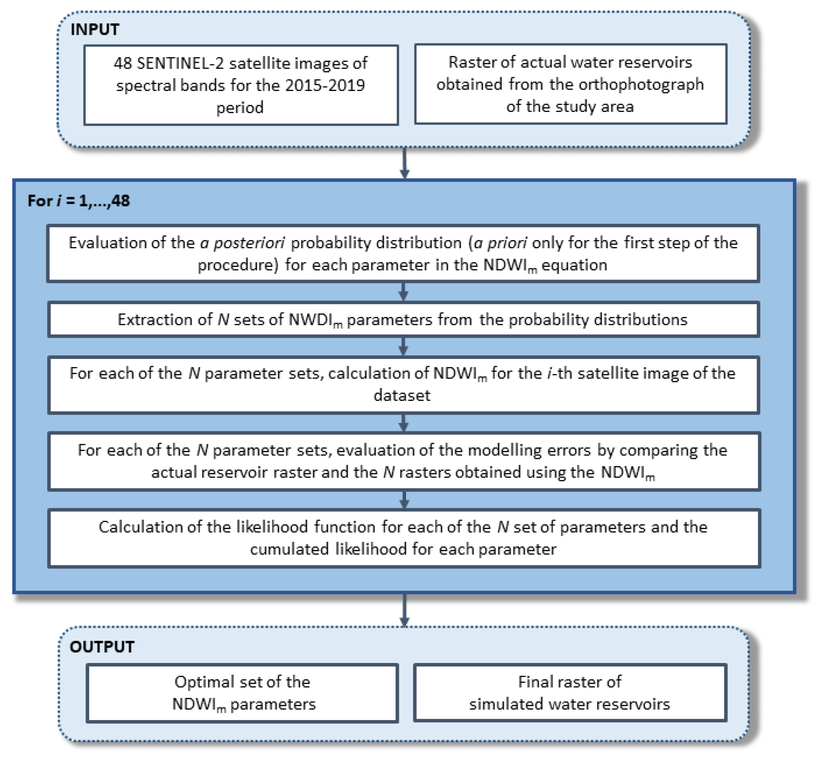
The procedure developed for the definition of the NDWIm parameters is briefly described by the flowchart in Figure 1.
The procedure proposed here can be summarized as follows:
- (1)
- First, 48 Sentinel-2 satellite images for bands 2, 3, 4, and 8, acquired in the 2015–2019 period, were collected. These data are spatially distributed over a 10 × 10 m cell grid. A raster with the same resolution was prepared by manually digitalizing the reservoirs currently located in the area of study.
- (2)
- For each of the parameters in Equation (2), a prior distribution was selected. Then, N values of each parameter were extracted from the prior distributions to create N sets of parameters.
- (3)
- Using the band images referred to in the first time step, the NDWIm was calculated N times for each cell of the 10 × 10 m grid. A threshold value equal to 1 was set to distinguish water cells (NDWIm ≥ 1) from non-water cells (NDWIm < 1). The residual errors were evaluated by comparing each of the N rasters of NDWIm and the raster of actual reservoirs.
- (4)
- Once residual errors were computed, a likelihood function was calculated for each of the N parameter sets.
Starting from the likelihood function, the posterior distribution for each parameter was estimated. Then, steps (2) to (4) were repeated for the following image set of the dataset up to the last. At point (2) of the procedure, each parameter of Equation (2) was picked up from a normal distribution (uninformative prior distribution). Repeating these extractions N times, N sets of parameters were generated. In this study, N was set equal to 300; therefore, the calculation of the NDWIm was performed 300 times for each of the images included in the dataset. To test the results, a value of the NDWIm was associated with a predicted reservoir raster with the same cell resolution as the actual reservoir raster. The comparison between the number of water grid cells in the actual reservoir raster and the number of water grid cells according to the calculation of the NDWIm provided the residual error x, which was evaluated as follows:
where Dw is the difference between the number of water grid cells in the actual reservoir raster and in the predicted reservoir raster, Dnw is the difference between the number of non-water grid cells in the actual reservoir raster and in the predicted reservoir raster, and T is the total number of grid cells. The analysis of residual errors allowed us to identify the probability distribution that provided the best fit and the proper likelihood function. Using Equation (3), 300 Monte Carlo simulations were run for computing the posterior distributions of parameters. Therefore, 300 sets of parameters were generated by extracting each parameter from the posterior distribution, and the NDWIm was calculated for the band images of the following time step. In summary, if m is the number of time steps in the dataset (four band images for each step), starting from the second time step, the likelihood function assessed for the (m − 1)-th step is used to evaluate the NDWIm parameters at the m-th step. In this way, uncertainty associated with the parameter assessment is recursively updated, along with the probabilistic distribution of the parameters, showing not only the most likely value of each parameter in the specific case but also the uncertainty related to its estimation (based on the probabilistic definition of Bayesian parameters).
2.3. Case Study and Dataset
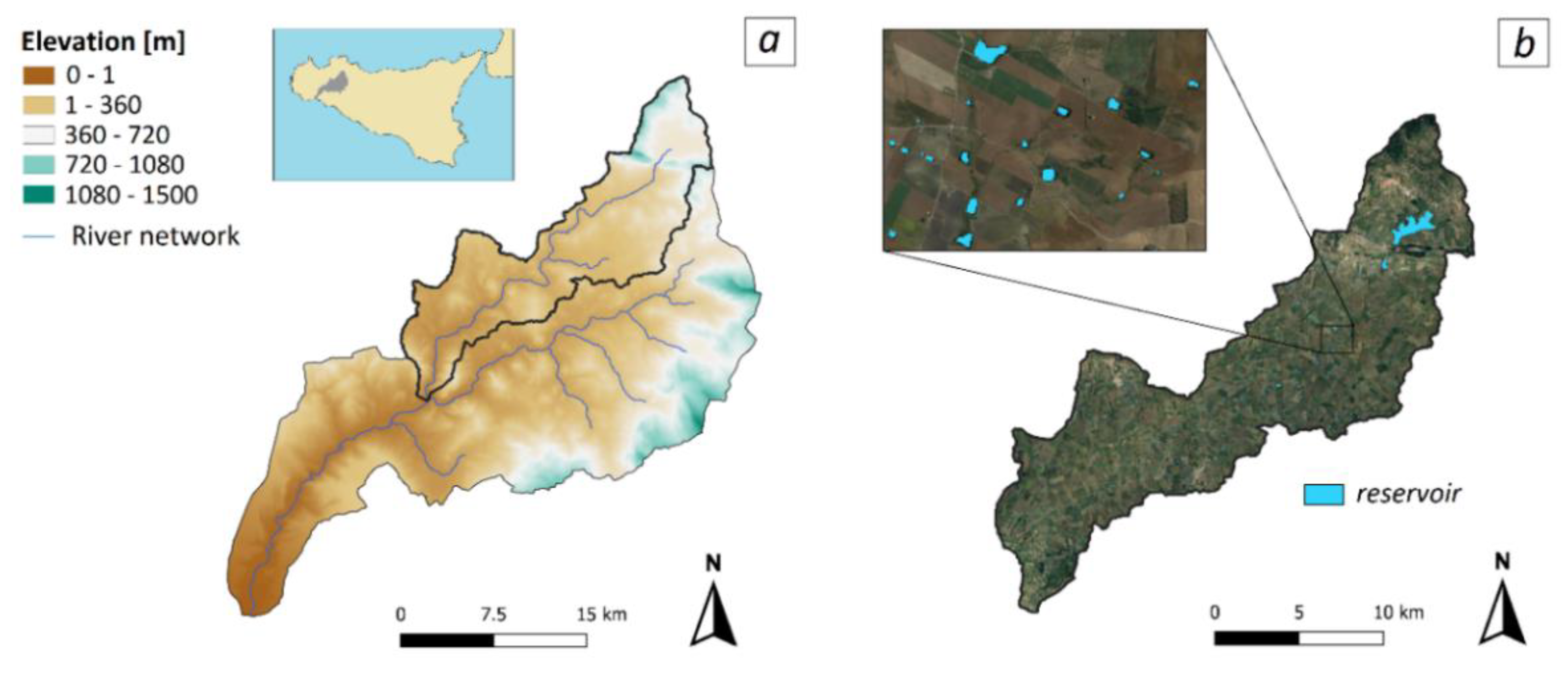
The study area is a subbasin of the Belice River catchment, located in Sicily (southern Italy). The subbasin is approximately 263 km2 (Figure 1a). In this area, land cover includes agricultural areas (99%), forest (0.9%), urban areas (0.05%), and water bodies (0.05%). A great number of small reservoirs for agricultural purposes and an artificial lake (Piana degli Albanesi Lake) are located in this area. In Figure 2b, the map of the reservoirs located in the subbasin is shown. This map was obtained by manually digitalizing the reservoirs visible in high-spatial resolution Google Earth images of the study area acquired on 11 June 2018. The dataset includes 440 actual reservoirs. The widest reservoir in the study area is Piana degli Albanesi Lake, an old artificial lake with a surface area of 1,700,000 m2. The remaining reservoirs have surfaces ranging from 20 m2 to 100,000 m2, with an average area of 2000 m2.
For the calculation of the NDWIm, 48 Sentinel-2 satellite images were used. The Sentinel-2 satellite is part of the Earth observation mission developed by the European Space Agency and designed for the global acquisition of multispectral images. Sentinel-2 provides spectral bands with different resolutions ranging from 10 to 60 m. Table 1 summarizes the characteristics of each Sentinel-2 spectral band. In this study, the 10-m resolution images for band 2 (blue), band 3 (green), band 4 (red), and band 8 (near infrared) recorded over the 2015–2019 period were collected. Sixty percent of the images were acquired during the summer months. The case study was selected because periodic surveys by the local water authority in the analyzed period state that no new reservoirs were built and no existing reservoir was dismissed in the 2015–2019 period. This choice removes the uncertainty related to the use of a single raster as reference data to validate the procedure. Moreover, seasonal variations of the water level slightly affect the extension of the reservoirs, which are characterized by small depths (approximately 5–6 m) and step banks (inclinations ranging from 45° to 60°). Due to their geometric characteristics, the reservoirs in the area of study are rarely completely dry.
3. Results and Discussion
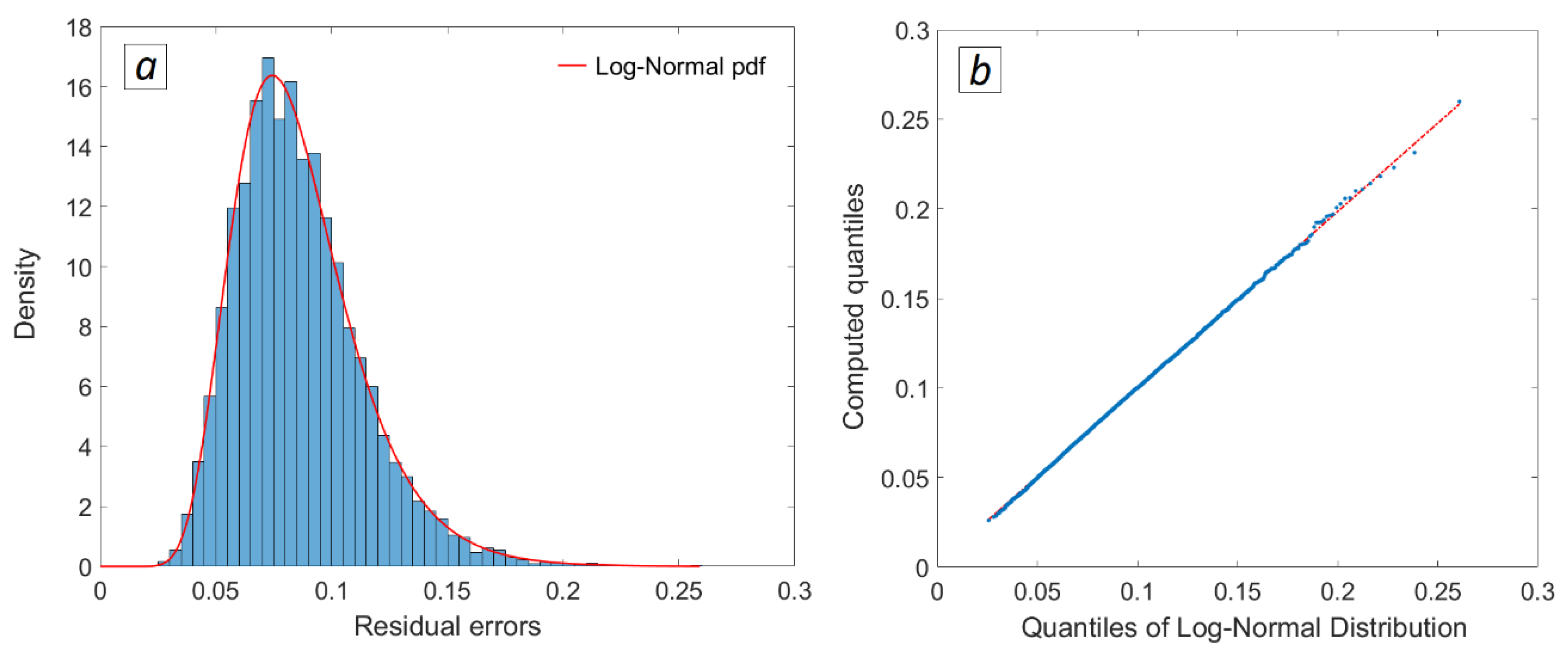
The Bayesian recursive approach described in Section 2.2 was applied to assess the parameters in Equation (2). Its application required the evaluation of the likelihood function in Equation (3). The normal likelihood function can be used under the assumption that the residual errors are independent, homoscedastic, and identically distributed in time. This hypothesis needs to be verified, and if the probability distribution of the residual errors cannot be fitted by a normal distribution, a different likelihood function must be introduced in Equation (3). In this study, the Kolmogorov–Smirnov test was applied to identify the probability distribution that provides the best fit for the residual errors, considering a significance level equal to 0.01. Among the tested probability distributions (normal, log-normal, exponential, Weibull, generalized extreme value, gamma, logistic, and log-logistic), the log-normal distribution properly described the residual errors. Therefore, to assess the posterior distribution, the following likelihood function was used:
where xn is the residual error and µ and σ2 are the mean and the variance of the residual errors, respectively. Figure 3a shows the frequency histogram of residual errors and the log-normal probability distribution function (PDF). Furthermore, a posterior diagnostic check was carried out to test the validity of the assumption of log-normal distributed residual errors. To this aim, the Q–Q plot was outlined comparing the empirical cumulative distribution function (CDF) of the residual error and the CDF of the log-normal distribution based on 5000 model estimates (Figure 3b). The results in Figure 3 show a reasonable fit of the chosen probability distribution to the residual errors.
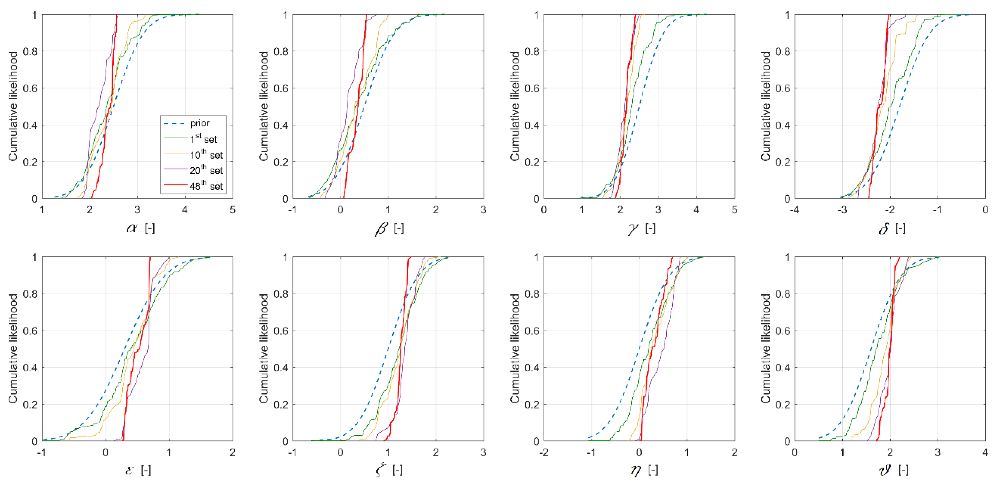
For the first set of spectral band images, the NDWIm was calculated using parameters extracted from prior distributions. The residual errors between the model and the observations at the first step allowed us to evaluate the likelihood function and, consequently, the posterior distributions from which the parameters for the following NDWIm calculation have to be picked up. Figure 4 shows the prior CDF (normal distribution) used for the first simulation set of the procedure and the CDF for some selected simulation sets up to the last (48th set). The variance in the posterior distribution decreases at each time step of the Bayesian recursive procedure. Indeed, the information assimilated by the model at each step gradually updates the uncertainty of predictions. Moreover, the influence of the prior distribution progressively decreases, as shown by the shape of the CDF, which is very similar to the normal CDF only for the 1st set.
The application of the proposed Bayesian approach produced a set of NDWIm parameters for each time step; therefore, a total of 48 sets was obtained. A maximum likelihood value was associated with each of these sets, ranging from 0.597 to 0.943. Lower values of maximum likelihood are related to the calculation of the NDWIm from spectral band images recorded during the autumn or winter months, for which cloud shadows in the images affect the reliability of model predictions.
The highest maximum likelihood was obtained using spectral band images acquired on 17 June 2017. Generally, input data recorded during the spring and summer months provided a maximum likelihood in the range 0.821 to 0.943. Based on the optimal set of NDWIm parameters, Equation (2) was modified as follows:
It has to be remarked that the parameterization of Equation (6) is the one which provides the highest value of maximum likelihood for the analyzed case of study. To ensure an optimal performance of the proposed index, the application of the Bayesian parameterization is suggested for each case of study to be investigated. The assessment of the parameters is not affected by the definition of the threshold, as discussed in Section 3.2.
3.1. Probability Distribution of Parameters
At the first step of the Bayesian procedure, it was assumed that all the parameters in Equation (2) were normally distributed. Therefore, the first set of parameters was generated by extracting the parameters from the normal PDF. In the following steps, parameters were picked up from the posterior distributions based on the assessment of the likelihood function.
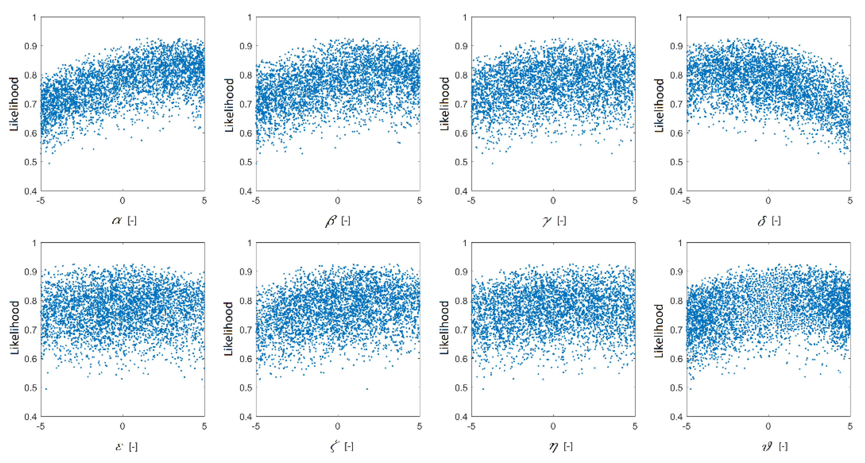
A sensitivity analysis was performed to detect which parameters were more influential. To this aim, considering the spectral images acquired on 17 June 2017, 5000 Monte Carlo simulations were run, and the related likelihood function was computed. Figure 5 shows the scatterplots of the likelihood function values for each parameter. In these plots, simulations with likelihood functions greater than 0.5 were included. The analysis of the scatterplots indicates that some parameters are more influential than others. Specifically, α and δ are the most sensitive parameters, while ε is the parameter that least affects the model prediction. Positive values of α are associated with higher values of the likelihood, while negative values of δ provided the best results. Likelihood function values up to 0.9 were obtained with ε values in all the considered ranges (from −5 to 5).
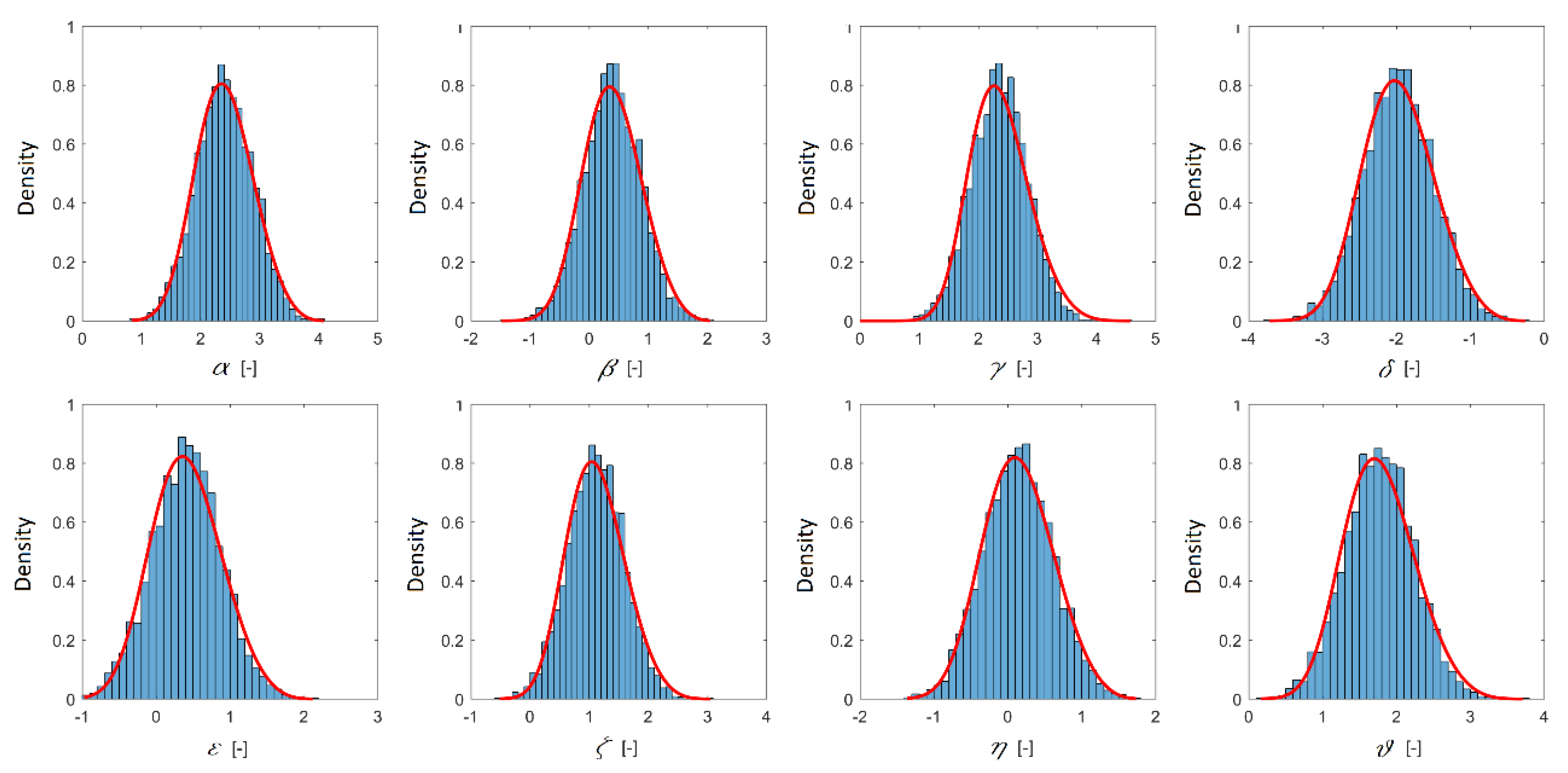
A goodness-of-fit analysis was also carried out for the parameter distributions. Following the same approach used for the analysis of residual errors, the Kolmogorov–Smirnov test was applied, and the Q–Q plots were outlined. The results indicated that, regardless of the assumption of a normal prior distribution, all the parameter distributions can be fitted by the generalized extreme value (GEV) probability distribution. In Figure 6, histograms of the parameters are plotted with the PDF of the GEV distribution.
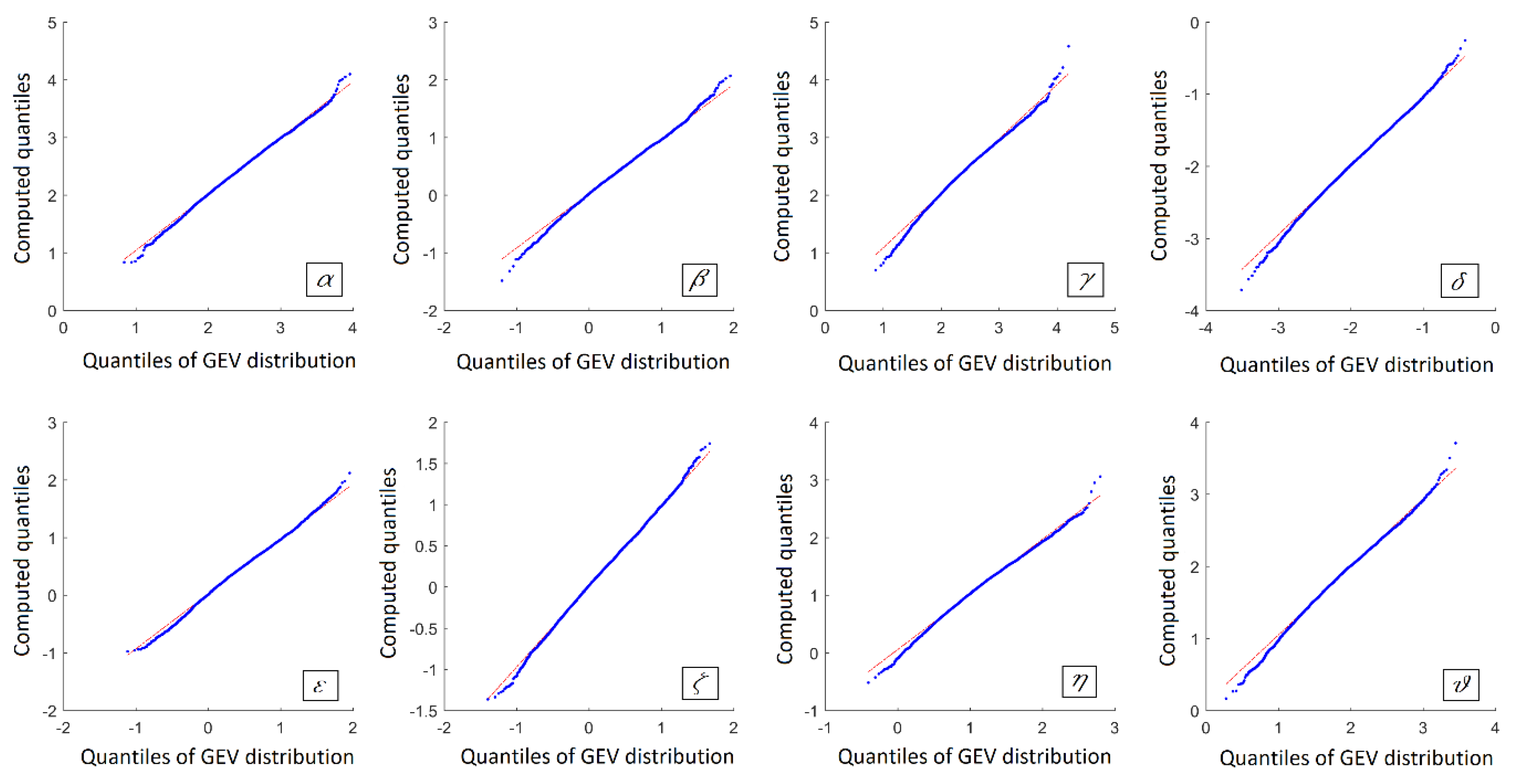
The Q–Q plots of the NDWIm parameters are shown in Figure 7. In all cases, the curves closely follow the bisectors, with a slight departure from the reference line only for the distribution tails. This result confirms that the GEV distribution provides a reliable fit for parameters.
3.2. Effects of the NDWIm Threshold on Parameterization
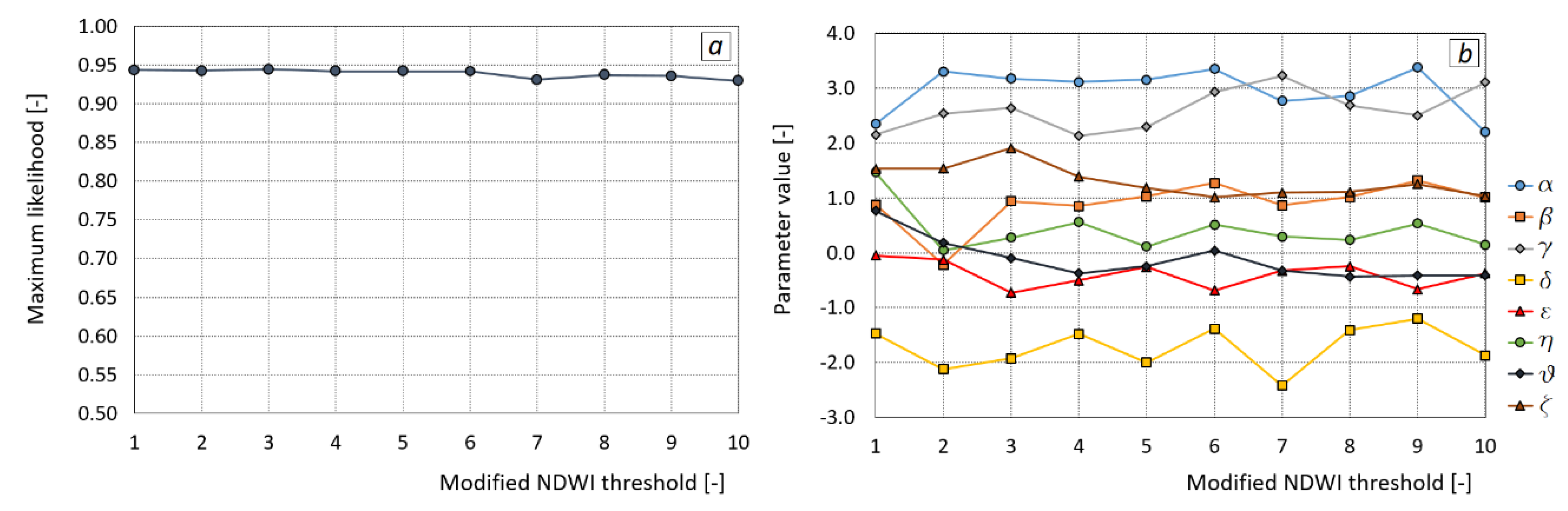
To achieve effective discrimination between water and non-water surfaces, the NDWIm threshold needs to be properly selected. In this study, a threshold equal to 1 was considered adequate to ensure an accurate detection of surface water features. This assumption was based on a preliminary analysis of the implications of the NDWIm threshold on the assessment of the parameters. To this aim, the application of the Bayesian procedure was repeated several times, considering ten different thresholds from 1 to 10. Figure 8a shows the variation in the maximum likelihood vs. the NDWIm threshold. The maximum likelihood undergoes a negligible reduction with the increase in the threshold, ranging from 0.924 to 0.943. The increase in the threshold does not improve the maximum likelihood and therefore does not produce any remarkable benefit in the parameterization of the NDWIm equation. This result is also confirmed by the moderate variation in the parameters associated with the maximum likelihood with the threshold. Figure 8b shows how sensitive the assessment of the parameters is to the choice of the threshold value. For each parameter, the range of variation is narrow.
3.3. Comparison between the NDWIm and NDWI
In this study, the performance of the proposed index was compared to that of the original formulation of the NDWI. As previously mentioned, the NDWIm threshold was set equal to 1, and this choice did not affect the parameterization of Equation (2). The comparison of the indexes required the definition of a reliable threshold for the NDWI. Some studies [2,5] suggested that the threshold of the NDWI can be set equal to zero. Nevertheless, this assumption can lead to overestimating or underestimating water surfaces since threshold values vary with the region and spectral band image. In the literature, frequency histograms were commonly used for threshold selection [21,34], whereas other researchers determined the NDWI threshold through the OTSU algorithm [27,35].
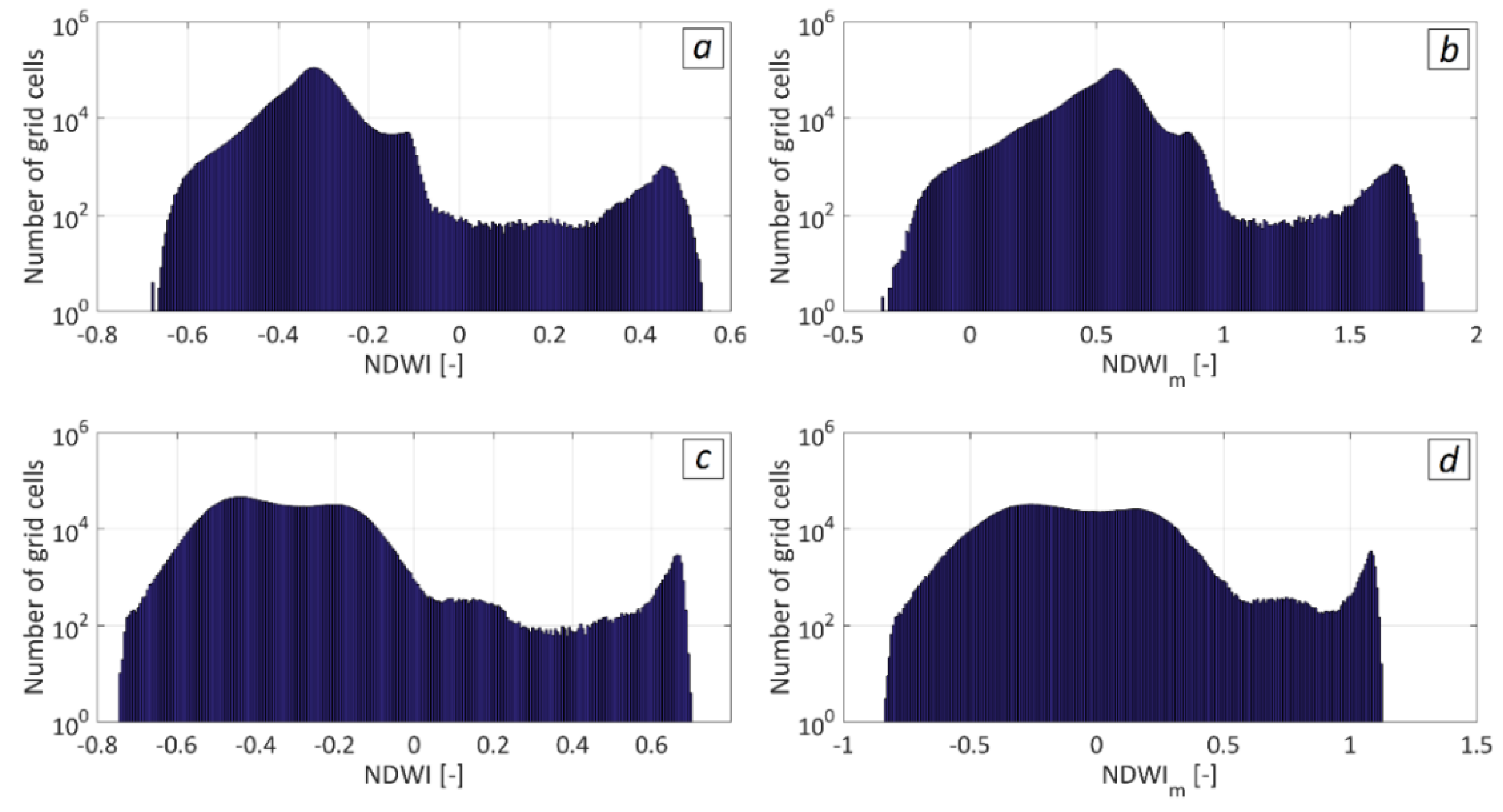
In this study, a preliminary analysis for the identification of the NDWI optimal threshold was carried out. As previously mentioned, frequency histograms can be successfully used for threshold optimization. Generally, the distribution of NDWI histograms is bimodal, and the threshold can be identified between the two peaks of water and non-water grid cells [10]. Nevertheless, in some cases, the distribution can be unimodal, and the identification of the threshold becomes more difficult. Figure 9 shows, in a semilogarithmic plot, the comparison between the frequency histograms of the NDWI and NDWIm calculated for the study area using the spectral band images acquired on 17 June 2017 and on 17 February 2019. As previously mentioned, the spectral images of 17 June 2017 are those that provided the highest maximum likelihood for the NDWIm, whereas the spectral images of 17 February 2019 provided the maximum likelihood difference between the NDWIm (0.87) and the NDWI (0.67). In Figure 9a,b, the two plots (images of 17 June 2017) display the same shape, but the ranges of variation in the indexes are different; specifically, the NDWI variations are between −0.681 and 0.556, while the NDWIm ranges between −0.349 and 1.791. Moreover, the NDWIm provides a sharper (less gradual) change in the value of the index, thus making it better for discriminating cells depending on value. The comparison between the plots in Figure 9c,d (images of 17 February 2019) highlights a slight difference in the shape of the frequency histograms. Indeed, both are bimodal, but in the histogram of the NDWI, an evident increase in grid cells in the range 0–0.2 occurred. In this case, for the images collected during winter, the calculation of the NDWI is more affected by shadow noise due to cloudiness; therefore, the number of grid cells that are classified as water, in a certain range of variation, is increased (more grid cells have an NDWI value greater than the threshold). However, the histogram of the NDWIm shows a decrease in the grid cells for which the index exceeds the threshold compared with that of Figure 9b. The NDWIm in Figure 9d is calculated with the set of parameters that provides the maximum likelihood for the images of 17 February 2019 and not the optimal set. In this case, the NDWIm is adequate for the classification of large reservoirs, while small water features are not recognized in most cases. However, the performance of the NDWIm is still better than that of the NDWI, as the number of false positives is not increased by cloud shadows in the images.
The semilogarithmic plot highlights a bimodal distribution, where the two peaks represent water and soil grid cells. The water area in the image is significantly smaller than the non-water area, and this difference makes recognition of the threshold more difficult. Therefore, the frequency histogram by itself could not be used effectively to identify the optimal NDWI threshold with high accuracy. For this reason, to distinguish between water and non-water cells, in this study, three different approaches were tested:
For the area of study, the first threshold appeared to be inadequate, excluding a considerable number of water cells (increase in false negative cases). According to the second method, for each set of images, an optimal threshold was selected by applying the Bayesian recursive method described in Section 2.2. Thus, for each set of images, the threshold linked to the maximum likelihood function value was chosen. Nevertheless, the results showed very high variability, with the value of the NDWI that discriminates water and non-water cells varying over a wide range (from −0.156 to 0.400). Finally, using the threshold suggested by Du et al. [27], water surfaces were effectively recognized by the NDWI values. For this reason, in this study, the NDWI threshold was set equal to 0.0759.
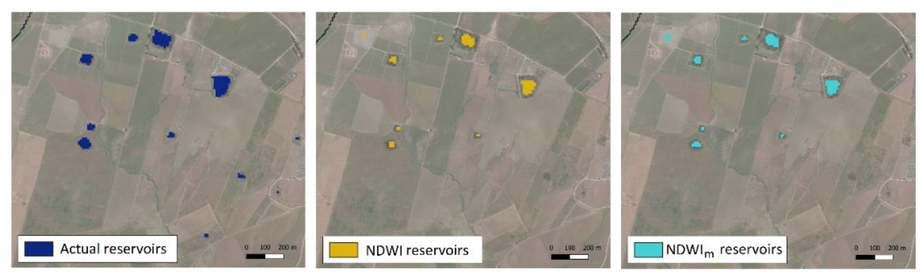
Figure 10 shows the comparison among three extracts of maps: one from the map of actual reservoirs and two from the maps of reservoirs predicted by the NDWI and NDWIm (calculated using the spectral images of 17 June 2017). Both indexes yielded a satisfactory performance, detecting most of the reservoirs. Nevertheless, the efficiency of the two indexes decreases for the smallest water surfaces in the area.
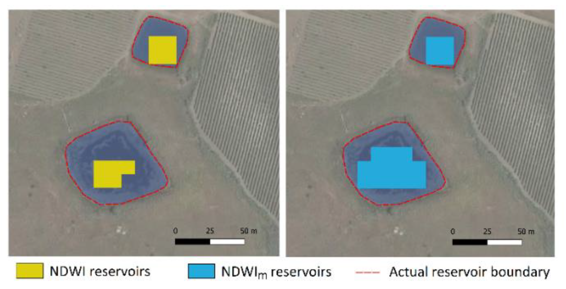
Figure 11 shows two details of the reservoir maps in Figure 10. As previously mentioned, the efficiency of both indexes decreases when small reservoirs have to be identified. Nevertheless, the NDWIm is more effective in the identification of water cells along the boundary of a reservoir. In Figure 11, for the smallest reservoir (100 m2), both indexes identify the same four cells as water, but for the other one (3000 m2), the NDWIm provided a better performance in the detection of the water cells along the boundary where the presence of vegetation usually reduces the effectiveness of water indexes in distinguishing water from wet vegetated soil.
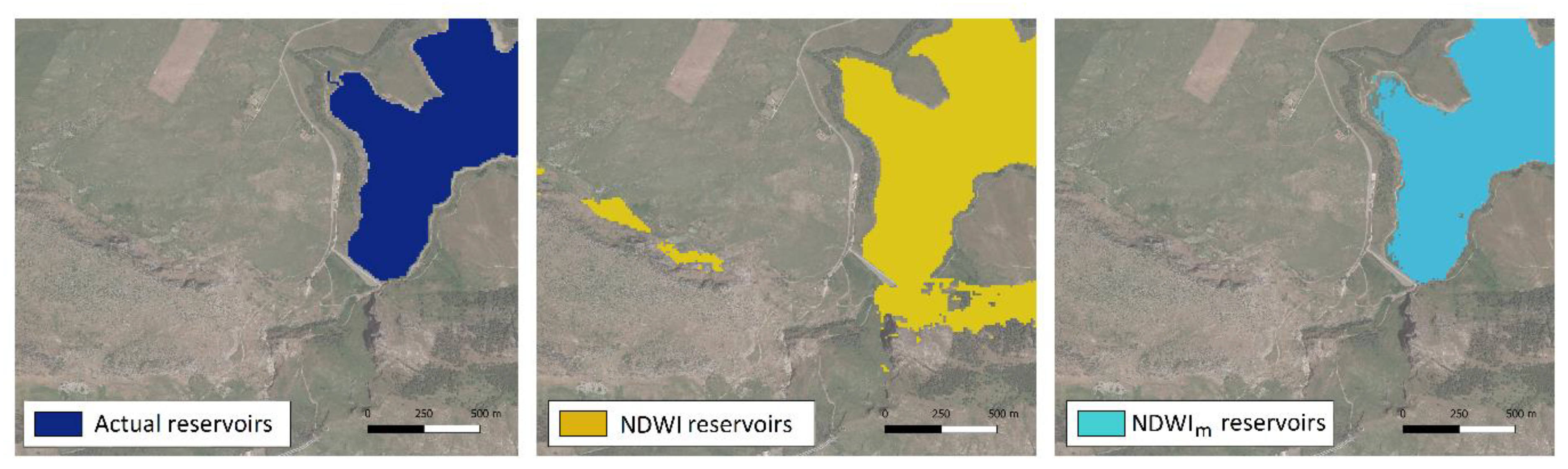
Figure 12 shows the same map extracts as in Figure 10, but indexes were calculated using the spectral images of 17 February 2019 and the related parameterization. As already pointed out by the frequency histograms in Figure 9, the NDWIm properly identifies the large reservoirs, with a lack of precision in the extraction of small water surfaces. Instead, the NDWI has a higher accuracy in classifying the small reservoirs as water, but it is more affected by shadow noises in imagery, providing a considerable number of false positives.
As a quantitative method to evaluate the efficiency of the indexes, a confusion matrix was created. The confusion matrix is commonly used to characterize image classification accuracy, comparing the predicted results with the reference image (the map of actual reservoirs). In this matrix, referring to the number of grid cells in the maps, true positive (TP), false positive (FP), true negative (TN), and false negative (FN) cases are reported. From the confusion matrix, two measures were derived: the overall accuracy and the Kappa coefficient [36]. The overall accuracy is the probability that a grid cell will be correctly classified as water by the index, calculated by dividing the sum of TP and TN cases by the total number of cases. Being affected by the dominating effect of the majority class, the overall accuracy by itself can be a misleading measure [37,38] since it may be quite high even if the model predictions are affected by a remarkable number of errors. Therefore, at least one other metric is required to have a thorough evaluation of the predictive performance. For this reason, the Kappa coefficient was computed using the following equation:
where T is the total number of grid cells and Σ is calculated as follows:
The Kappa coefficient is a single value metric that gives an overall assessment between the classification and the reference data. Specifically, it measures the agreement between two raters (also known as “judges” or “observers”) which classify categorical items into mutually exclusive classes. Similar to correlation coefficients, the index takes values from 0 to 1. A Kappa coefficient equal to zero indicates that there is no agreement between the model predictions and the reference image. Thus, the higher the Kappa coefficient is, the more accurate the prediction. Kappa equal to 1 represents the perfect agreement between prediction and reference data. Table 2 shows the confusion matrix calculated for the map of NDWI-predicted reservoirs. The overall accuracy is equal to 99.700%, and the Kappa coefficient is equal to 0.825.
In Table 3, the confusion matrix calculated for the map of NDWIm-predicted reservoirs is shown. The overall accuracy is equal to 99.711%, and the Kappa coefficient is equal to 0.837. Comparing the results in Table 2 and Table 3, a slight reduction in FN cases and a moderate increase in FP cases can be observed. The NDWI is more precise in the identification of non-water grid cells (higher number of TN cases), while the NDWIm is more effective in discriminating water grid cells (higher number of TP cases).
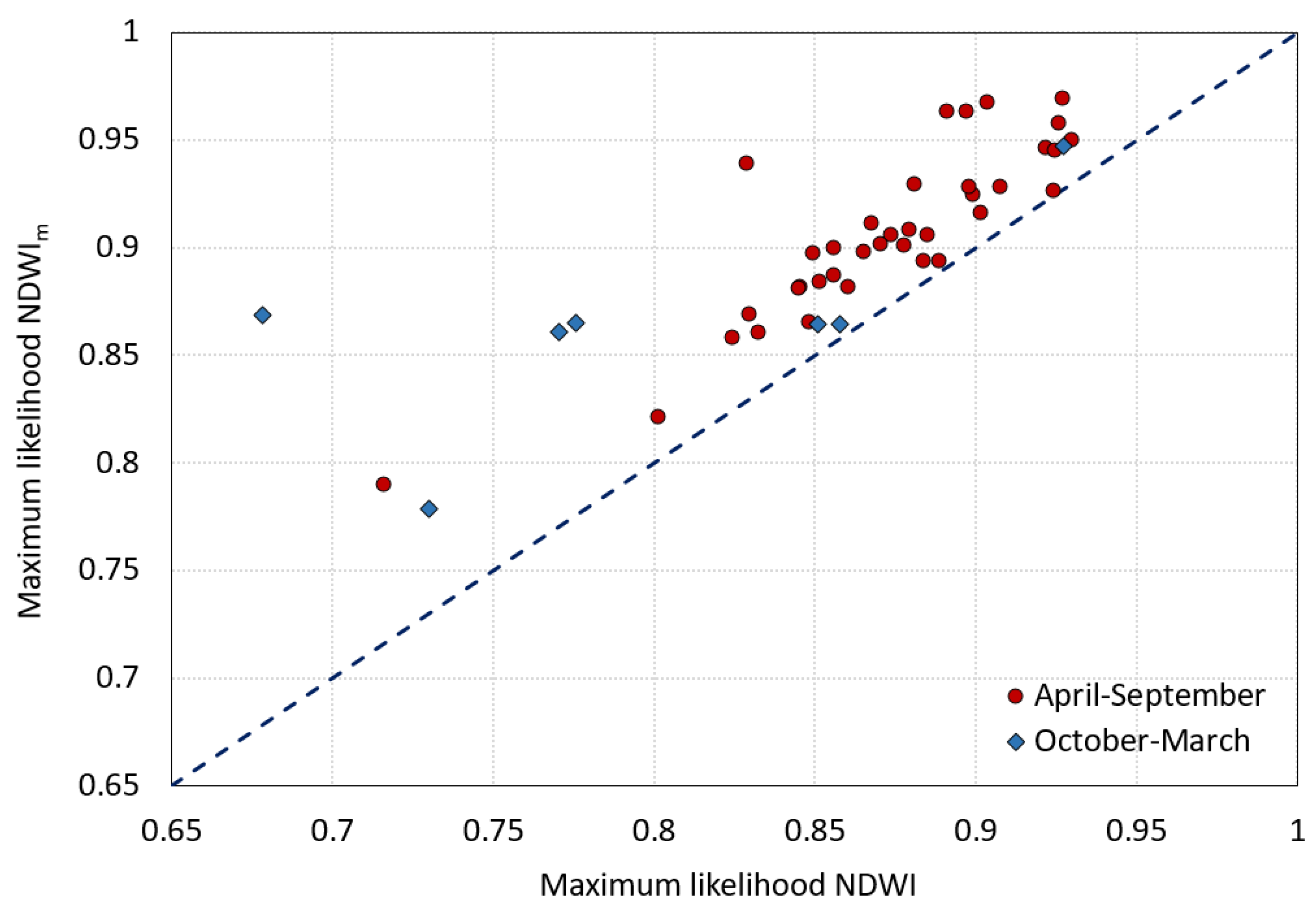
Finally, a comparison between the performance of the NDWI and NDWIm, in terms of maximum likelihood, was carried out. Figure 13 shows the plot of the maximum likelihood for the NDWI vs. the maximum likelihood for the NDWIm calculated from the same set of spectral images. Thus, the plot includes 48 points, distinguishing imagery acquired during the April–September period from imagery acquired during the October–March period. All the points are above the reference line, with the maximum likelihood of the NDWIm being greater than that of the NDWI for each set of images. Results in Figure 13 show that the Bayesian parameterization makes the the NDWIm performance more robust and reliable than that of the NDWI in terms of maximum likelihood. Moreover, for the analyzed case of study, the optimal set of parameters does not need to be updated when new spectral band images are available whereas the use of the NDWI requires the calibration of the threshold each time new information is acquired.
It has to be remarked that the optimal parameter set here assessed is not valid for any other area of study. Thus, the use of the proposed index to other cases requires the application of the Bayesian parameterization procedure to detect the optimal parameters. The parameterization of the index also needs to be performed when different satellite images are used (e.g. LANDSAT), due to their specific characteristics and spatial resolution.
4. Conclusions
The accurate identification of surface water features over a region is essential for multiple purposes, including water resource management and flood risk assessment. To this aim, in recent decades, reliable and robust methodologies for mapping surface water have been developed, supported by the availability of remote sensing technologies and, consequently, the accessibility to high-resolution multispectral satellite images. The NDWI was extensively used to delineate surface bodies even if its application requires the definition of a threshold to distinguish between water and non-water features in a satellite image. This threshold can be affected by multiple factors, depending on the quality of the image to be processed.
In this study, the NDWIm was developed and applied for the detection of reservoirs in a small catchment in southern Italy. Even if a calibrated threshold is not needed for the proposed index, its computation is based on the estimation of eight parameters.
The uncertainty related to a given model prediction is the result of the combined effects of the input data, model structure, and model parameters. Therefore, reducing the uncertainty associated with the parameter assessment can considerably improve the model predictions. In this study, the use of a Bayesian recursive procedure allowed us to describe the uncertainty related to parameter estimation in terms of probability. Specifically, the parameterization of the NDWIm was based on the estimation of the posterior probability distributions of the parameters, which were updated at each step of the procedure by the assimilation of new remote sensing data.
The performance of the novel index was compared to that of the original formulation of the NDWI, as proposed in [2], in terms of the overall accuracy and Kappa coefficient. The results showed that the NDWIm is suitable for extracting surface water information, overlooking the issues related to the quality of the satellite images used for the calculation and to the definition of an optimal threshold.
The comparison between the overall accuracy of the NDWI and NDWIm indicated that the performances of the two indexes are quite similar in terms of overall accuracy and Kappa coefficient. Nevertheless, the use of the proposed index, together with the Bayesian parameterization procedure, has some substantial advantages compared with those of other indexes in the literature used for surface water detection, such as the NDWI. First, the NDWIm threshold does not need to be calibrated, whereas the use of the NDWI requires the selection of the optimal threshold for each processed image. Moreover, the accuracy of the NDWIm in surface water detection is not affected by the quality of the spectral band images. The dataset used in this study includes images acquired not only in spring and summer but also in autumn and winter when the shadow noise due to cloudiness is more relevant. The use of indexes in the literature usually requires the application of algorithms for the enhancement of image quality and, consequently, the improvement of extraction precision [9,39]. The Bayesian parameterization of the NDWIm ensures more robustness to the methodology, reducing the implication of dataset quality on the results. Despite the effectiveness of the NDWIm in the extraction of surface water features, the index lacks precision in the detection of very small reservoirs. Indeed, most of the reservoirs with surface areas between 20 m2 and 500 m2 are not detected by the index, and variations in the threshold do not improve the NDWIm precision.
In this study, a reference image of actual reservoirs was obtained by manually digitalizing the reservoirs visible in high-spatial resolution Google Earth images of the study area. Reservoirs in the area of study are affected by slight seasonal variations, therefore, the reference map can be considered quite representative of the actual reservoirs in the catchment. It has to be remarked that, to ensure a reliable performance of the proposed procedure, the use of an accurate reference image for testing the effectiveness of the index is highly recommended when the reservoirs in the area of interest are subjected to seasonal or annual variations.
Further developments of this study could include the investigation of the capacity of the NDWIm in the delineation of flooded areas. Indeed, flood monitoring and the related damage assessment could be effectively supported by the use of the proposed index.
Author Contributions
Conceptualization, G.F., L.L., S.N., and V.P.; methodology, G.F. and S.N.; formal analysis, G.F. and L.L.; investigation, G.F., L.L., S.N., and V.P.; data curation, S.N.; writing—original draft preparation, L.L., V.P., and G.F.; writing—review and editing, G.F., L.L., and V.P.; visualization, L.L.; supervision, G.F. All authors have read and agreed to the published version of the manuscript.
Funding
This research received partial financial support from the Italian Ministry of Environment by means of the project “LIMNADI—Integrazione muLti-scopo di piccoli Invasi collinari per la laMiNAzione Delle pIene”—CUP B76C18000890001.
Conflicts of Interest
The authors declare no conflicts of interest.
References
- Ji, L.; Zhang, L.; Wylie, B.K. Analysis of Dynamic Thresholds for the Normalized Difference Water Index. Photogramm. Eng. Remote Sens. 2009, 75, 1307–1317. [Google Scholar] [CrossRef]
- McFeeters, S.K. The use of the Normalized Difference Water Index (NDWI) in the delineation of open water features. Int. J. Remote Sens. 1996, 17, 1425–1432. [Google Scholar] [CrossRef]
- Gao, B.-C. NDWI—A normalized difference water index for remote sensing of vegetation liquid water from space. Remote Sens. Environ. 1996, 58, 257–266. [Google Scholar] [CrossRef]
- Rogers, A.S.; Kearney, M.S. Reducing signature variability in unmixing coastal marsh Thematic Mapper scenes using spectral indices. Int. J. Remote Sens. 2004, 25, 2317–2335. [Google Scholar] [CrossRef]
- Xu, H. Modification of normalised difference water index (NDWI) to enhance open water features in remotely sensed imagery. Int. J. Remote Sens. 2006, 27, 3025–3033. [Google Scholar] [CrossRef]
- Rallo, G.; Minacapilli, M.; Ciraolo, G.; Provenzano, G. Detecting crop water status in mature olive groves using vegetation spectral measurements. Biosyst. Eng. 2014, 128, 52–68. [Google Scholar] [CrossRef]
- Ma, M.; Wang, X.; Veroustraete, F.; Dong, L. Change in area of Ebinur Lake during the 1998–2005 period. Int. J. Remote Sens. 2007, 28, 5523–5533. [Google Scholar] [CrossRef]
- Campos, J.C.; Sillero, N.; Brito, J.C. Normalized difference water indexes have dissimilar performances in detecting seasonal and permanent water in the Sahara–Sahel transition zone. J. Hydrol. 2012, 464, 438–446. [Google Scholar] [CrossRef]
- Rokni, K.; Ahmad, A.; Selamat, A.; Hazini, S. Water Feature Extraction and Change Detection Using Multitemporal Landsat Imagery. Remote Sens. 2014, 6, 4173–4189. [Google Scholar] [CrossRef] [Green Version]
- Liu, Z.; Yao, Z.; Wang, R. Assessing methods of identifying open water bodies using Landsat 8 OLI imagery. Environ. Earth Sci. 2016, 75. [Google Scholar] [CrossRef]
- Soti, V.; Tran, A.; Bailly, J.-S.; Puech, C.; Seen, D.L.; Bégué, A. Assessing optical earth observation systems for mapping and monitoring temporary ponds in arid areas. Int. J. Appl. Earth Obs. Geoinf. 2009, 11, 344–351. [Google Scholar] [CrossRef] [Green Version]
- Shum, C.K.; Howat, I.M.; Larour, E.; Husby, E.; Husby, E. Coastline extraction from repeat high resolution satellite imagery. Remote Sens. Environ. 2019, 229, 260–270. [Google Scholar] [CrossRef]
- Yang, L.; Tian, S.; Yu, L.; Ye, F.; Qian, J.; Qian, Y. Deep learning for extracting water body from Landsat imagery. Int. J. Innov. Comput. Inf. Control. 2015, 11, 1913–1929. [Google Scholar]
- Yang, J.; Du, X. An enhanced water index in extracting water bodies from Landsat TM imagery. Ann. GIS 2017, 23, 1–8. [Google Scholar] [CrossRef]
- Jain, S.K.; Singh, R.D.; Jain, M.; Lohani, A.K. Delineation of Flood-Prone Areas Using Remote Sensing Techniques. Water Resour. Manag. 2005, 19, 333–347. [Google Scholar] [CrossRef]
- Ogashawara, I.; Curtarelli, M.P.; Ferreira, C.M. The use of optical remote sensing for mapping flooded areas. Int. J. Eng. Res. Appl. 2013, 3, 1956–1960. [Google Scholar]
- Amarnath, G. An algorithm for rapid flood inundation mapping from optical data using a reflectance differencing technique. J. Flood Risk Manag. 2013, 7, 239–250. [Google Scholar] [CrossRef]
- Memon, A.A.; Muhammad, S.; Rahman, S.; Haq, M. Flood monitoring and damage assessment using water indices: A case study of Pakistan flood-2012. Egypt. J. Remote Sens. Space Sci. 2015, 18, 99–106. [Google Scholar] [CrossRef] [Green Version]
- Liebe, J.; Van De Giesen, N.; Andreini, M.; Steenhuis, T.S.; Walter, M. Suitability and Limitations of ENVISAT ASAR for Monitoring Small Reservoirs in a Semiarid Area. IEEE Trans. Geosci. Remote Sens. 2008, 47, 1536–1547. [Google Scholar] [CrossRef]
- Liebe, J.; Van De Giesen, N.; Andreini, M. Estimation of small reservoir storage capacities in a semi-arid environment. Phys. Chem. Earth Parts A/B/C 2005, 30, 448–454. [Google Scholar] [CrossRef]
- Lacaux, J.-P.; Tourre, Y.; Vignolles, C.; Ndione, J.; Lafaye, M. Classification of ponds from high-spatial resolution remote sensing: Application to Rift Valley Fever epidemics in Senegal. Remote Sens. Environ. 2007, 106, 66–74. [Google Scholar] [CrossRef]
- Cao, M.; Zhou, H.; Zhang, C.; Zhang, A.; Li, H.; Yang, Y. Research and application of flood detention modeling for ponds and small reservoirs based on remote sensing data. Sci. China Ser. E Technol. Sci. 2011, 54, 2138–2144. [Google Scholar] [CrossRef]
- Annor, F.; Van De Giesen, N.; Liebe, J.; Van De Zaag, P.; Tilmant, A.; Odai, S. Delineation of small reservoirs using radar imagery in a semi-arid environment: A case study in the upper east region of Ghana. Phys. Chem. Earth Parts A/B/C 2009, 34, 309–315. [Google Scholar] [CrossRef] [Green Version]
- Amitrano, D.; Di Martino, G.; Iodice, A.; Riccio, D.; Ruello, G. Small Reservoirs Extraction in Semiarid Regions Using Multitemporal Synthetic Aperture Radar Images. IEEE J. Sel. Top. Appl. Earth Obs. Remote Sens. 2017, 10, 3482–3492. [Google Scholar] [CrossRef]
- McFeeters, S.K. Using the Normalized Difference Water Index (NDWI) within a Geographic Information System to Detect Swimming Pools for Mosquito Abatement: A Practical Approach. Remote Sens. 2013, 5, 3544–3561. [Google Scholar] [CrossRef] [Green Version]
- Liu, Y.; Song, P.; Peng, J.; Ye, C. A physical explanation of the variation in threshold for delineating terrestrial water surfaces from multi-temporal images: Effects of radiometric correction. Int. J. Remote Sens. 2012, 33, 5862–5875. [Google Scholar] [CrossRef]
- Du, Y.; Zhang, Y.; Ling, F.; Wang, Q.; Li, W.; Li, X. Water Bodies’ Mapping from Sentinel-2 Imagery with Modified Normalized Difference Water Index at 10-m Spatial Resolution Produced by Sharpening the SWIR Band. Remote Sens. 2016, 8, 354. [Google Scholar] [CrossRef] [Green Version]
- Kaplan, G.; Avdan, U. Object-based water body extraction model using Sentinel-2 satellite imagery. Eur. J. Remote Sens. 2017, 50, 137–143. [Google Scholar] [CrossRef] [Green Version]
- Bayes, T. LII. An essay towards solving a problem in the doctrine of chances. By the late Rev. Mr. Bayes, F. R. S. communicated by Mr. Price, in a letter to John Canton, A. M. F. R. S. Philos. Trans. R. Soc. Lond. 1763, 53, 370–418. [Google Scholar] [CrossRef]
- Fernandes, W.; Naghettini, M.; Loschi, R.H. A Bayesian approach for estimating extreme flood probabilities with upper-bounded distribution functions. Stoch. Environ. Res. Risk Assess. 2010, 24, 1127–1143. [Google Scholar] [CrossRef]
- Freni, G.; Mannina, G. Bayesian approach for uncertainty quantification in water quality modelling: The influence of prior distribution. J. Hydrol. 2010, 392, 31–39. [Google Scholar] [CrossRef] [Green Version]
- Schoups, G.; Vrugt, J.A. A formal likelihood function for parameter and predictive inference of hydrologic models with correlated, heteroscedastic, and non-Gaussian errors. Water Resour. Res. 2010, 46. [Google Scholar] [CrossRef] [Green Version]
- Smith, T.; Sharma, A.; Marshall, L.; Mehrotra, R.; Sisson, S.A. Development of a formal likelihood function for improved Bayesian inference of ephemeral catchments. Water Resour. Res. 2010, 46. [Google Scholar] [CrossRef] [Green Version]
- Li, J.; Sheng, Y. An automated scheme for glacial lake dynamics mapping using Landsat imagery and digital elevation models: A case study in the Himalayas. Int. J. Remote Sens. 2012, 33, 5194–5213. [Google Scholar] [CrossRef]
- Li, W.; Du, Z.; Ling, F.; Zhou, D.; Wang, H.; Gui, Y.; Sun, B.; Zhang, X. A Comparison of Land Surface Water Mapping Using the Normalized Difference Water Index from TM, ETM+ and ALI. Remote Sens. 2013, 5, 5530–5549. [Google Scholar] [CrossRef] [Green Version]
- Cohen, J. A Coefficient of Agreement for Nominal Scales. Educ. Psychol. Meas. 1960, 20, 37–46. [Google Scholar] [CrossRef]
- Fitzgerald, R.; Lees, B. Assessing the classification accuracy of multisource remote sensing data. Remote Sens. Environ. 1994, 47, 362–368. [Google Scholar] [CrossRef]
- Stehman, S.V. Selecting and interpreting measures of thematic classification accuracy. Remote Sens. Environ. 1997, 62, 77–89. [Google Scholar] [CrossRef]
- Jawak, S.; Luis, A. Spectral Information Analysis for the Semiautomatic Derivation of Shallow Lake Bathymetry Using High-resolution Multispectral Imagery: A Case Study of Antarctic Coastal Oasis. Aquat. Procedia 2015, 4, 1331–1338. [Google Scholar] [CrossRef]
- Li, Y.; Gao, H.; Jasinski, M.F.; Zhang, S.; Stoll, J. Deriving High-Resolution Reservoir Bathymetry From ICESat-2 Prototype Photon-Counting Lidar and Landsat Imagery. IEEE Trans. Geosci. Remote Sens. 2019, 57, 7883–7893. [Google Scholar] [CrossRef]
- Li, Y.; Gao, H.; Zhao, G.; Tseng, K.H. A high-resolution bathymetry dataset for global reservoirs using multi-source satellite imagery and altimetry. Remote Sens. Environ. 2020, 244, 111831. [Google Scholar] [CrossRef]
Figure 1.
Flowchart of the proposed procedure.

Figure 2.
(a) Digital elevation model (DEM) of the Belice River basin and the analyzed subbasin and (b) map of reservoirs in the subbasin.
Figure 2.
(a) Digital elevation model (DEM) of the Belice River basin and the analyzed subbasin and (b) map of reservoirs in the subbasin.

Figure 3.
(a) Histogram of residual errors and log-normal PDF and (b) Q–Q plot of residual errors.

Figure 4.
CDF of likelihood for the prior distribution and for a selection of simulation sets for each NDWIm parameter.
Figure 4.
CDF of likelihood for the prior distribution and for a selection of simulation sets for each NDWIm parameter.

Figure 5.
Scatterplots of the likelihood function for NDWIm parameters.

Figure 6.
Histograms of NDWIm parameters and GEV PDF.

Figure 7.
Q–Q plots of NDWIm parameters.

Figure 8.
(a) Variation in maximum likelihood vs. NDWIm threshold and (b) variation in parameter values vs. NDWIm threshold.
Figure 8.
(a) Variation in maximum likelihood vs. NDWIm threshold and (b) variation in parameter values vs. NDWIm threshold.

Figure 9.
Frequency histograms: (a) NDWI for 17 June 2017; (b) NDWIm for 17 June 2017; (c) NDWI for 17 February 2019; and (d) NDWIm for 17 February 2019.
Figure 9.
Frequency histograms: (a) NDWI for 17 June 2017; (b) NDWIm for 17 June 2017; (c) NDWI for 17 February 2019; and (d) NDWIm for 17 February 2019.

Figure 10.
Comparison between the map of actual reservoirs and the maps of reservoirs predicted by the NDWI and NDWIm (17 June 2017).
Figure 10.
Comparison between the map of actual reservoirs and the maps of reservoirs predicted by the NDWI and NDWIm (17 June 2017).

Figure 11.
Details of the reservoir maps in Figure 10. For the reservoir at the bottom of the images, the NDWIm is more effective in detecting the water cells along the boundary of the water body.
Figure 11.
Details of the reservoir maps in Figure 10. For the reservoir at the bottom of the images, the NDWIm is more effective in detecting the water cells along the boundary of the water body.

Figure 12.
Comparison between the map of actual reservoirs and the maps of reservoirs predicted by the NDWI and NDWIm (17 February 2019).
Figure 12.
Comparison between the map of actual reservoirs and the maps of reservoirs predicted by the NDWI and NDWIm (17 February 2019).

Figure 13.
Maximum likelihood of the NDWI vs. the maximum likelihood of the NDWIm.


Table 1.
Central wavelength and spatial resolution of Sentinel-2 imagery.
| Number | Description | Central Wavelength | Resolution |
|---|---|---|---|
| (μm) | (m) | ||
| B1 | Coastal aerosol | 0.443 | 60 |
| B2 | Blue | 0.490 | 10 |
| B3 | Green | 0.560 | 10 |
| B4 | Red | 0.665 | 10 |
| B5 | Red edge 1 | 0.705 | 20 |
| B6 | Red edge 2 | 0.740 | 20 |
| B7 | Red edge | 0.783 | 20 |
| B8 | Near infrared (NIR) | 0.842 | 10 |
| B8A | Near infrared narrow (NIRn) | 0.865 | 20 |
| B9 | Water vapor | 0.945 | 60 |
| B10 | Shortwave infrared (SWIR)-Cirrius | 1.375 | 60 |
| B11 | Shortwave infrared 1 (SWIR1) | 1.610 | 20 |
| B12 | Shortwave infrared 2 (SWIR2) | 2.190 | 20 |
Table 2.
Confusion matrix for the NDWI.
| Actual | Predicted | |
|---|---|---|
| Positive | Negative | |
| Positive | 18,813 | 6912 |
| Negative | 981 | 2,602,803 |
Table 3.
Confusion matrix for the NDWIm.
| Actual | Predicted | |
|---|---|---|
| Positive | Negative | |
| Positive | 19,736 | 5989 |
| Negative | 1623 | 2,602,098 |
© 2020 by the authors. Licensee MDPI, Basel, Switzerland. This article is an open access article distributed under the terms and conditions of the Creative Commons Attribution (CC BY) license (http://creativecommons.org/licenses/by/4.0/).
Share and Cite
MDPI and ACS Style
Liuzzo, L.; Puleo, V.; Nizza, S.; Freni, G. Parameterization of a Bayesian Normalized Difference Water Index for Surface Water Detection. Geosciences 2020, 10, 260. https://0-doi-org.brum.beds.ac.uk/10.3390/geosciences10070260
AMA Style
Liuzzo L, Puleo V, Nizza S, Freni G. Parameterization of a Bayesian Normalized Difference Water Index for Surface Water Detection. Geosciences. 2020; 10(7):260. https://0-doi-org.brum.beds.ac.uk/10.3390/geosciences10070260
Chicago/Turabian StyleLiuzzo, Lorena, Valeria Puleo, Salvatore Nizza, and Gabriele Freni. 2020. "Parameterization of a Bayesian Normalized Difference Water Index for Surface Water Detection" Geosciences 10, no. 7: 260. https://0-doi-org.brum.beds.ac.uk/10.3390/geosciences10070260
Note that from the first issue of 2016, this journal uses article numbers instead of page numbers. See further details here.