Seismic Reflection Methods in Offshore Groundwater Research


1
Department of Earth Sciences, University of Oxford, South Parks Road, Oxford OX1 3AN, UK
2
Université de Montpellier, CNRS, Université des Antilles, Place E. Bataillon, 34095 Montpellier, France
3
Helmholtz Centre for Ocean Research, GEOMAR, 24148 Kiel, Germany
4
Marine Geology & Seafloor Surveying, Department of Geosciences, University of Malta, MSD 2080 Msida, Malta
5
CDM Smith Ireland Ltd., D02 WK10 Dublin, Ireland
*
Author to whom correspondence should be addressed.
Geosciences 2020, 10(8), 299; https://0-doi-org.brum.beds.ac.uk/10.3390/geosciences10080299
Submission received: 8 April 2020
/
Revised: 13 July 2020
/
Accepted: 26 July 2020
/
Published: 5 August 2020
Abstract
:There is growing evidence that passive margin sediments in offshore settings host large volumes of fresh and brackish water of meteoric origin in submarine sub-surface reservoirs. Marine geophysical methods, in particular seismic reflection data, can help characterize offshore hydrogeological systems and yet the existing global database of industrial basin wide surveys remains untapped in this context. In this paper we highlight the importance of these data in groundwater exploration, by reviewing existing studies that apply physical stratigraphy and morpho-structural interpretation techniques to provide important information on—reservoir (aquifer) properties and architecture, permeability barriers, paleo-continental environments, sea-level changes and shift of coastal facies through time and conduits for water flow. We then evaluate the scientific and applied relevance of such methodology within a holistic workflow for offshore groundwater research.
1. Introduction
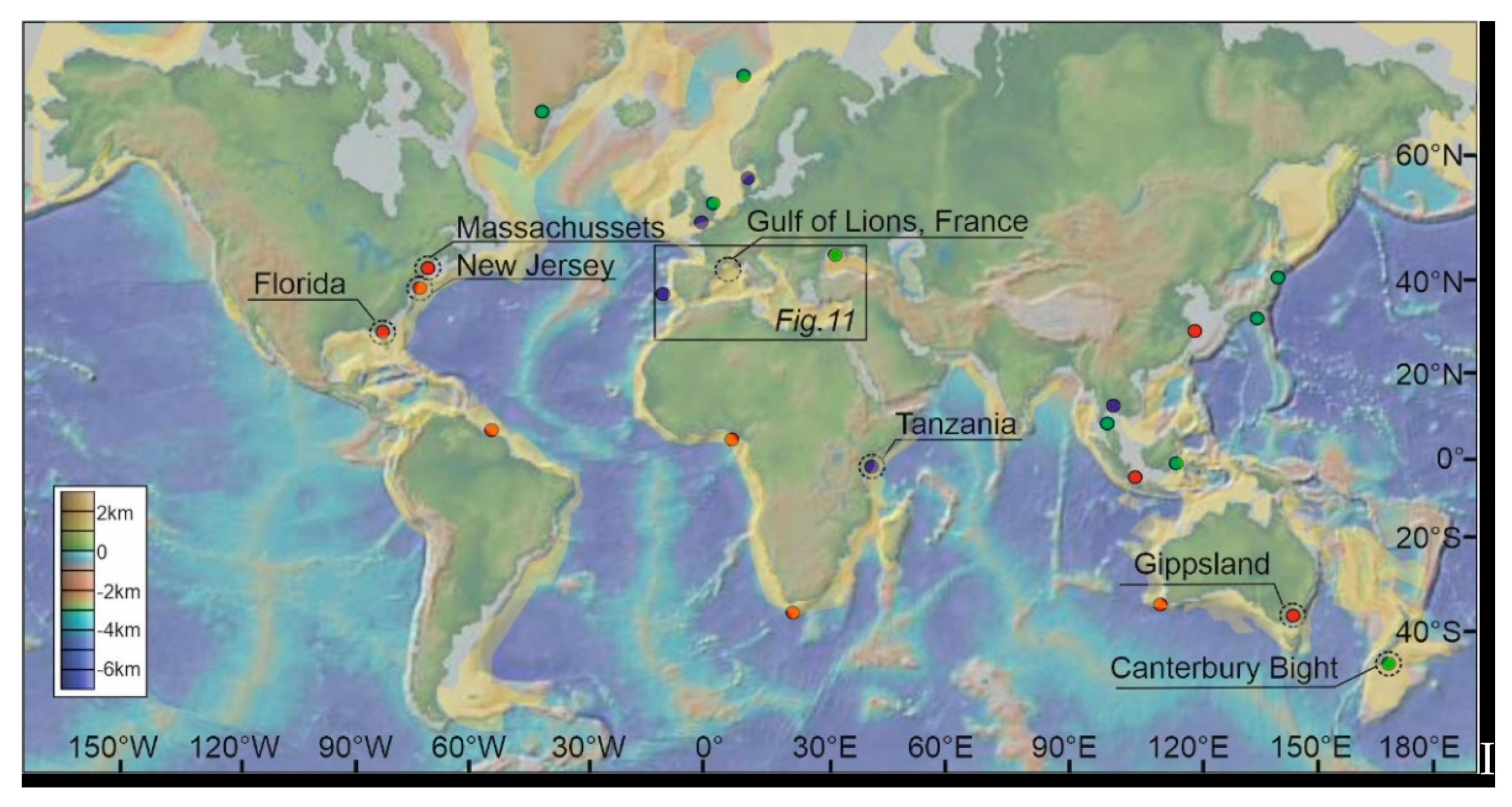
Groundwater resources are declining due to over-exploitation and climate change [1]. In particular, present-day sea-level rise and over-pumping are threatening the availability of freshwater in coastal areas [2,3], where aquifers are experiencing a high level of depletion, saline contamination and pollution from agricultural, urban and industrial activities [4,5,6,7,8,9,10,11,12,13]. In the last decade, there has been growing evidence that passive margin sediments in offshore settings can host large volumes of low salinity water in sub-surface reservoirs (Figure 1) [4,14,15,16,17,18,19,20]. Current calculations based on averaged aquifer properties on worldwide continental shelves estimate that the volume of brackish (<10 g/L) water stored in passive margins worldwide is approximately 5 × 10⁵ km3; this number decreases to 3 × 10⁵ km3 if considering water of <1 g/L [4,16]. However, this estimate includes only 16% of the present-day coastline.
The presence of low salinity water in the shallow offshore might produce an economic advantage for countries that rely heavily on desalinization as their main source of freshwater. The economic costs of this expensive process could considerably decrease by the use of extracted water with lower salt content. Therefore, there is a mounting interest in producing accurate maps of offshore groundwater resources, determine their likely responses to climate and sea-level changes and assess how much water they could sustainably supply, especially in proximity of water-stressed coastal cities [21].
1.1. Distribution of Offshore Groundwater
Offshore groundwater is composed of meteoric-derived water, compaction-driven fluids and thermobaric-derived fluids [22]. Shallow and proximal sediments (at 10 s to few 100 s m of seabed and burial depths) on continental shelves contain pore fluids that are dominated by water of meteoric origin, flowing in a basinward direction [23]. Deeper sediments up to few 1000 s of meters of burial depth contain pore fluids, of higher salinity, expelled by compaction in a landward and upward direction. Occasionally, the presence of fresh or low salinity fluids in the marine subsurface is linked to the expulsion of diagenetic fluids from sediments such as evaporites, clays and silica [24,25,26,27,28]. Thermobaric derived fluids are present at higher depths (see summary in Reference [22]).
Of these offshore groundwater systems, topographically driven meteoric recharge (TDM), that is, a combination of rainfall recharge and topographically driven flow, is the most important driver for the emplacement of fresh or low salinity (also defined as ‘freshened’) water in continental shelves and upper slopes of passive margins [29,30,31]. In these systems, the offshore reach of modern coastal aquifers into the submarine realm is constrained by a flow cell system with recharge from land. This depends on whether the onshore water table is high enough to provide the necessary driving force and whether there is hydraulic connectivity between the offshore aquifer and the onshore recharge area (see e.g., References [4,32]). Land-derived groundwater can be transported by conduits in sub-sea sediments or by pore-water flow in sediments of sufficient porosity and permeability (see e.g., Reference [33]). Groundwater may discharge directly on the seafloor through submarine groundwater discharge (SGD) [30,34,35,36,37,38,39].
These processes alone, however, do not explain the large volumes of low-salinity groundwater that are found across continental shelves [4]. Offshore low-salinity groundwater accumulations, not necessarily connected to onshore recharge areas, can also be stored in confined paleo-aquifers. These are generally paleo-freshwater of meteoric origin, trapped in sediments during past times of lower sea level (see e.g., Reference [40]). These accumulations do not appear in global resources calculations but potentially also represent a large volume of deeply stored fresh-water.
Submarine groundwater is mostly studied along the shallower part of passive continental margins, with some notable exceptions on convergent margins [38,41]. On continental margins, submarine groundwater is usually stored in sedimentary rocks, in two main lithological groups—carbonate and siliciclastic. Both groups are covered by the case studies presented in this paper. The geological age of the sediments hosting the aquifers is variable but generally not older than Cenozoic. This could be related to data bias towards shallower sedimentary sequences, the higher potential for offshore aquifers hosting TDM and to the much higher probability of preservation/permanence of freshened water aquifers in the last few thousands of years [40,42].
1.2. Methods and Approaches to the Study of Offshore Groundwater
A combination of geological, geophysical, hydrogeological, petrophysical and hydrogeological data provide essential information for the study of offshore groundwater. These include:
- Active source, multi-channel reflection seismic (hereby referred to simply as ‘seismic data’);
- Electromagnetics (EM, CSEM);
- Seabed mapping tools (multibeam, water column backscatter, side-scan sonar and LIDAR);
- Thermal remote sensing;
- Sediment core and pore water geochemical analyses;
- Borehole geophysics, imaging and hydrogeology (e.g., spontaneous potential, nuclear magnetic resonance, resistivity, flow-meters, etc.).
Offshore data acquisition presents logistical and technical challenges and it is generally more costly than onshore operations. For example, in clastic systems, coring is often problematic at shallow depth on continental shelves, due to the difficulty of drilling through poorly consolidated and coarse-grained sediments and possible presence of overpressured horizons [15]. Consequently, many studies of large-scale offshore groundwater circulation largely rely on modelling. However, accurate flow models primarily depend on the correct estimation of rock permeability and stratigraphic organization, which define the presence or absence of groundwater reservoirs and the modes of groundwater/seawater exchange.
Seismic reflection data, which are the focus of this paper, constitute an effective tool to map reservoir properties (especially in siliciclastic reservoirs) at a large scale, to reconstruct past sea level and environmental changes and support the analysis of the response of aquifers to these events. Thus, seismic reflection data can play an important role in the global identification of offshore freshened groundwater and potential resources, as one of the components of a workflow which includes the methods described above.
Our main aims are—to describe how seismic data can be used within this workflow, to study offshore groundwater and help identify potential low-salinity aquifers; to review the key case studies where seismic reflection data have been integrated into offshore groundwater analysis (either acquired on purpose or subsequently made available for such studies); and to discuss the limitations and future potential of such approach, both for scientific and applied purposes.
2. Seismic Reflection Data
Seismic data provide information on subsurface geology both in two dimensions (2D seismic), through individual vertical cross sections and in three-dimensions (3D seismic) through areal coverage of subsurface geological structures, generally down to kilometers in depth. Chirp profiling systems are used to acquire ultra-high resolutions for shallower depths [43,44,45,46,47]. In this review we present examples of both high-resolution, shallow penetration 2D datasets and lower resolution, deeper penetration 2D datasets.
Shallow, high-resolution (few centimeters to few meters) seismic data have been used, often serendipitously, to help characterize offshore groundwater systems, mostly located on passive continental margins [4,16,17]. The focus of this seismic method has been on stratigraphic architecture, facies prediction and identification of past sea level and environmental changes that might have affected paleo-aquifers. Conversely, deep penetration and lower resolution (in the order of 10 s of meters) seismic reflection data are routinely acquired and processed in industry (mostly oil and gas) and more occasionally, in academia. They have a deeper sub-surface imaging capability (several kilometers) and are used to interpret geology, structure and stratigraphy of continental margins (Figure 1), while they have been rarely applied to the analysis of offshore groundwater. In the few studies where this has been done, seismic data have been used for the interpretation of the large scale basin evolution and architecture, including the definition of lithological and stratigraphic units and structural elements, rather than direct imaging of aquifers. This global database already exists; therefore, it can potentially spur new studies in previously unexplored areas.
2.1. Seismic Stratigraphy, Sequence Stratigraphy and Attribute Analysis
The interpretation methods most relevant or more used in offshore groundwater analysis include physical stratigraphy and morpho-structural interpretation. Seismic and sequence stratigraphic interpretation techniques are disciplines of the physical stratigraphy that emerged in the late 1970s [48,49,50,51,52,53,54], predominantly focused on siliciclastic continental margins and subsequently on carbonate [55,56,57] and continental (e.g., Reference [58]) environments. A wide literature exists on the applications of those initial concepts and their evolution in most marine basins worldwide [59,60,61,62], as well as the use of seismic data for the stratigraphic analysis of continental margins [48,49,50,51,52,53,54,63,64,65,66].
The dominant ‘eustatic paradigm’ of the original sequence stratigraphic concepts [65,67] has been subsequently expanded to include the variability of systems tract and other units related to (1) tectonics, driving relative sea-level changes and accommodation space, at a local, crustal [59,60,61] and lithospheric scale; (e.g., Reference [59]) and (2) lateral variability caused by depositional and erosional irregularities (e.g., Reference [62]).
Seismic and sequence stratigraphic methods are broadly based on the identification and mapping of reflection geometries, terminations and seismic facies, systems tracts and sequences/sequence boundaries. Horizon-based interpretation can be combined with attribute analysis, both pre- and post-stack, which include trace attributes (e.g., amplitude, magnitude, continuity, frequency) or horizon/time attributes (e.g., dip, azimuth, curvature). Attribute analysis may support the interpretation of stratigraphic bodies, facies and discontinuities. Well tie, when available, leads to the cross-borehole physical properties of the sediments throughout the extent of the seismic data. Figure 2 shows an example of this methodology applied to offshore groundwater research. Quantitative seismic methods are instead used to understand amplitude variations, mostly relevant as a validation of hydrocarbon anomalies but also to provide additional information for reservoir characterization [68]. The most important of these techniques include post-stack amplitude analysis (bright-spot and dim-spot analysis for fluid content identification), offset-dependent amplitude analysis (AVO analysis), acoustic and elastic impedance inversion and forward seismic modeling [69].
2.2. Seismic Morpho-Structural Interpretation
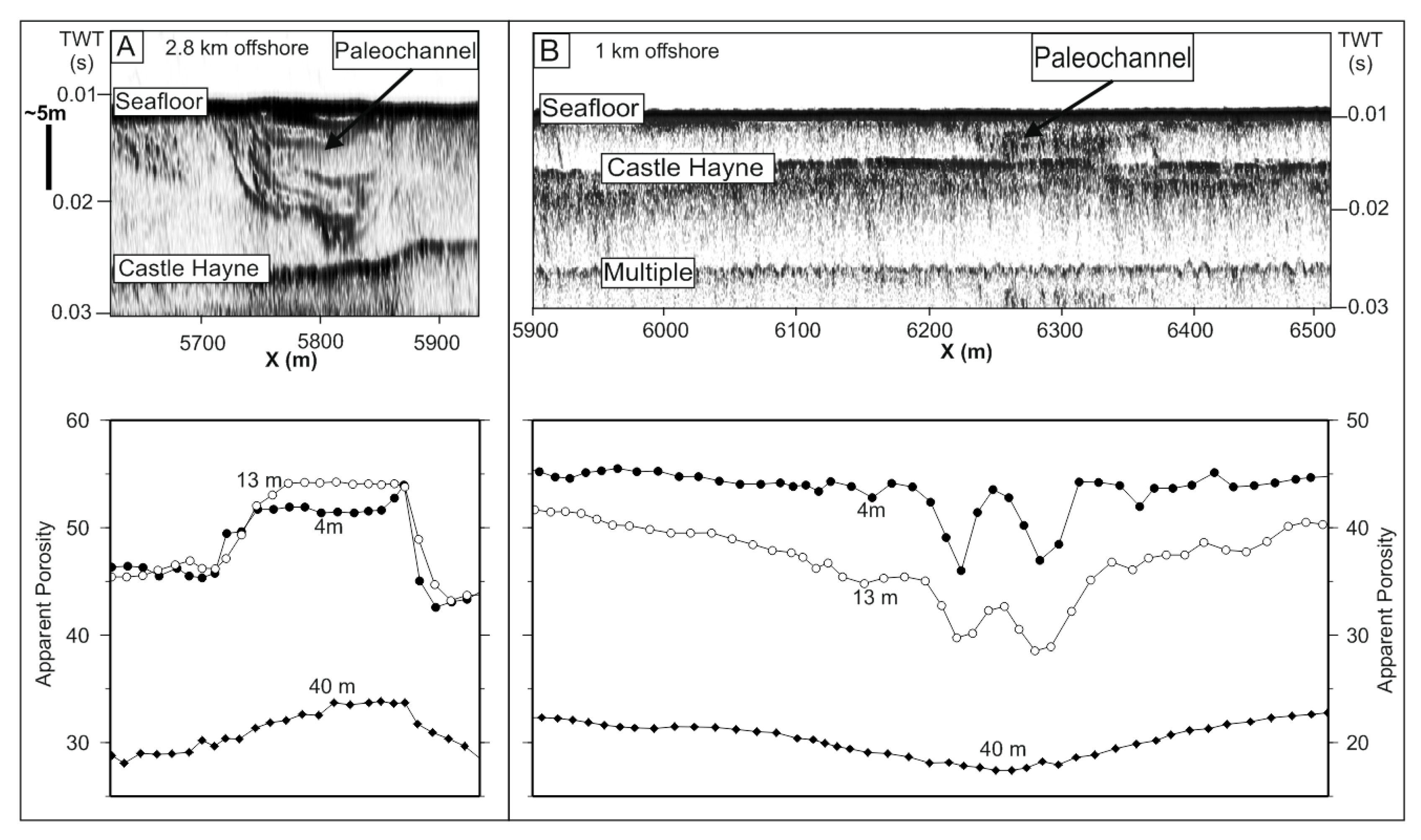
On the seabed and in the subsurface, seismic data can image specific geomorphological and structural features which are relevant for the interpretation of the presence of freshened groundwater environments [47]. Examples are (paleo)channels and canyons [72,73,74] (Figure 3), sinkholes and other dissolution-related karstic features [75,76,77], pockmarks, pipes [78,79] and faults.
Buried channels and canyons can contribute to submarine groundwater discharge by serving as conduits for pore water flow [74], if they breach confining units and their infill is composed of permeable sediments. An example is offshore North Carolina, where based on simulation modeling and offshore geophysical data, the authors suggest that pore water of intermediate salinity is present in paleochannel sediments (Figure 3).
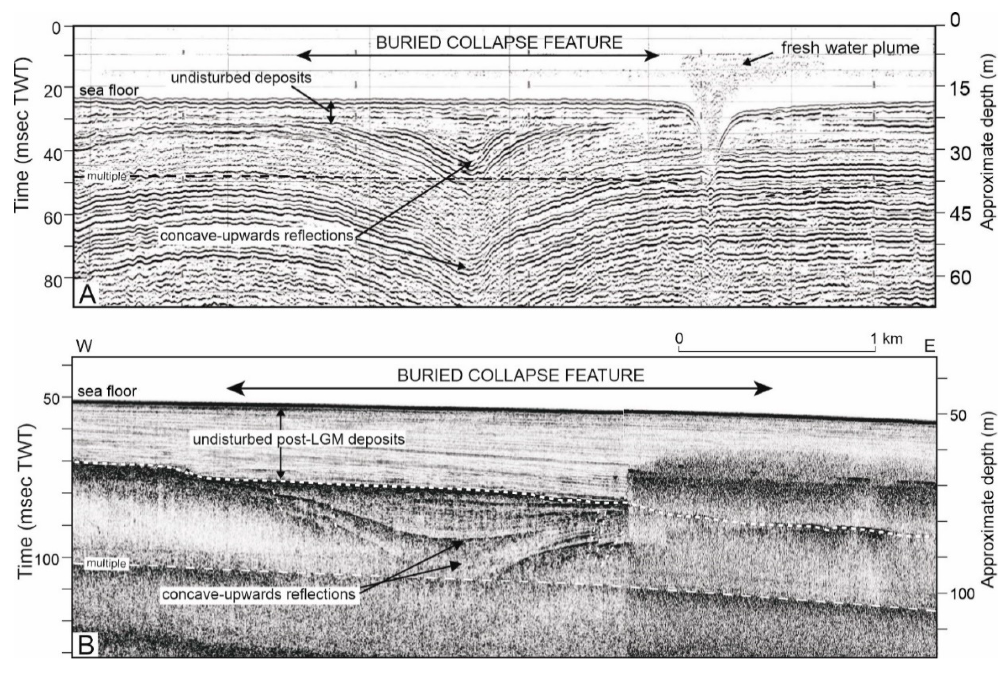
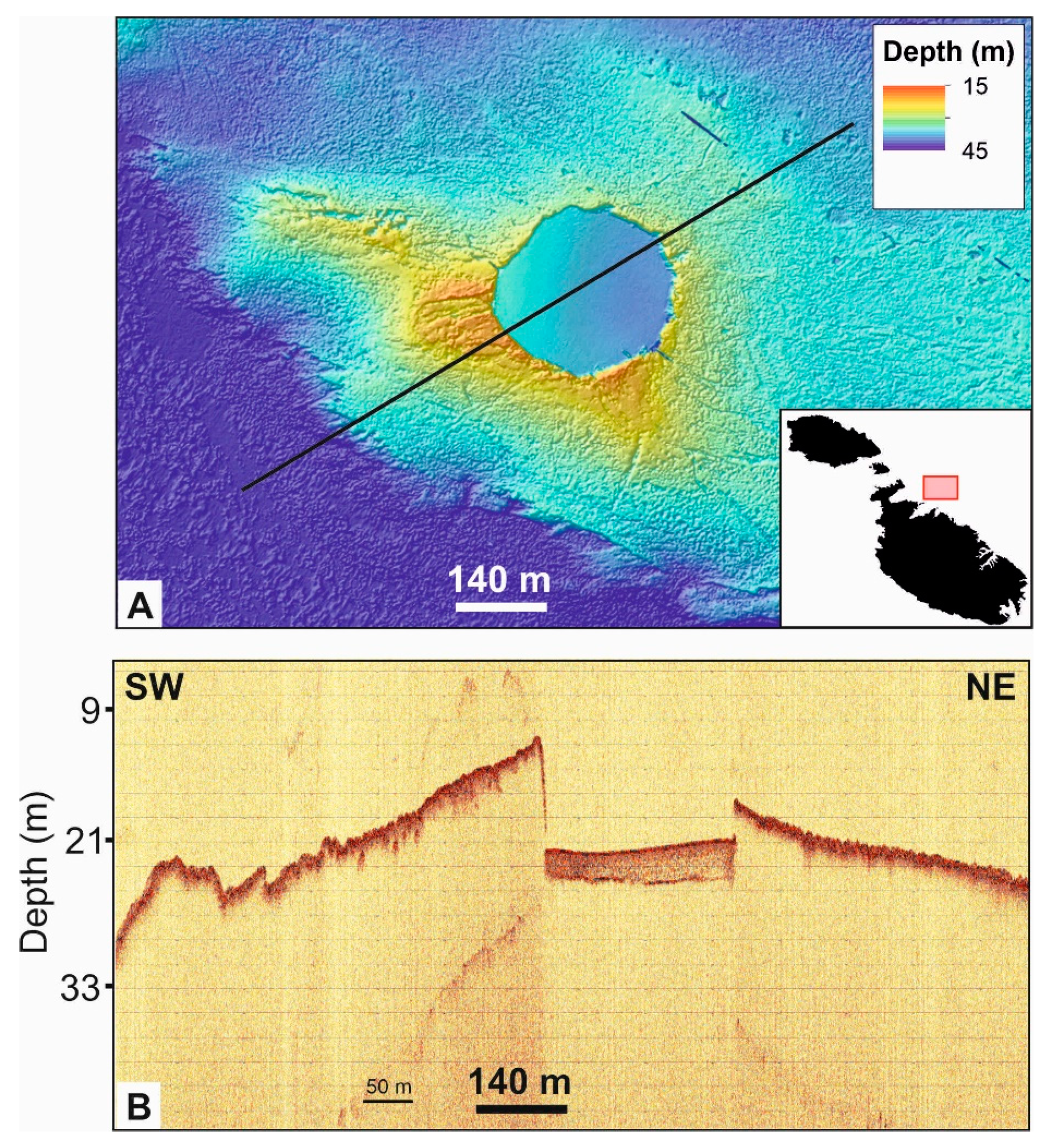
In karstic terrains, substratum dissolution can create sinkholes and other morphologies that favor groundwater flow. If the sinkholes are buried, seismic data can be used to recognize whether they are active or fossil and if they have been subject to multiple collapse phases (Figure 4). The presence of poly-phase solution-subsidence⁄collapse structures associated to deep palaeo-karst conduits can be linked to repeated sea-level low-stands (Figure 4) [76]. Eustatic variations can also favor dissolution, as changes in hydraulic gradient, related to the elevation difference, potentially lead to increase in karstification [80] (Figure 5). Limestone corrosion resulting from mixing of fresh and salt waters occurs in proximal offshore environments [81,82,83]. The presence of these features is detected on seismic data and can be used as an indication of paleo freshwater tables in limestones.
Large non-eustatic sea level drops can also be recorded by coastal karstic springs and their linked conduits. An example is the dramatic drop in sea-level that occurred in the Mediterranean during the Messinian salinity crisis, ca. 6 Million years ago [85,86,87,88] which left seismic evidence of conduits extending to a considerable depth below the last glacial maximum lowstand.
Pockmarks and pipes are diagnostic features for the occurrence of focused and vertical fluid flow [78]. This type of fluid flow is caused by upwards flowing gas and/or pore water [89,90]. Pockmarks are also present in lacustrine environments, such as in Lake Neuchatel (Switzerland), where they have been related to the expulsion of fresh pore waters and to active fluid flow by karstic groundwater discharge from the Jura Mountain front into the Swiss Plateau Hydrological system [91]. Finally, faults and associated structural interpretation of seismic data can indicate the presence of fractured reservoirs and potential flow conduits or lateral permeability barriers.
3. Case Studies
We present a series of key studies that show how seismic data have been used to aid interpretation of offshore groundwater systems, with a focus on low-salinity (fresh or freshened) aquifers. For each of these case studies, we focus on results or contributions from seismic stratigraphic methods and morpho-structural interpretation, based on the criteria and examples described in Section 2.1 and Section 2.2.
3.1. North Atlantic Margin
The North Atlantic margin (location in Figure 1) is a site of primary interest in the field of submarine groundwater research. In this area, offshore groundwater bodies hosting large amounts of low salinity submarine pore water have been discovered [15,92].
3.1.1. New Jersey
In this case study, we show how seismic methods have been used for reservoir and seal characterization and fault conduit interpretation in a siliciclastic passive margin setting.
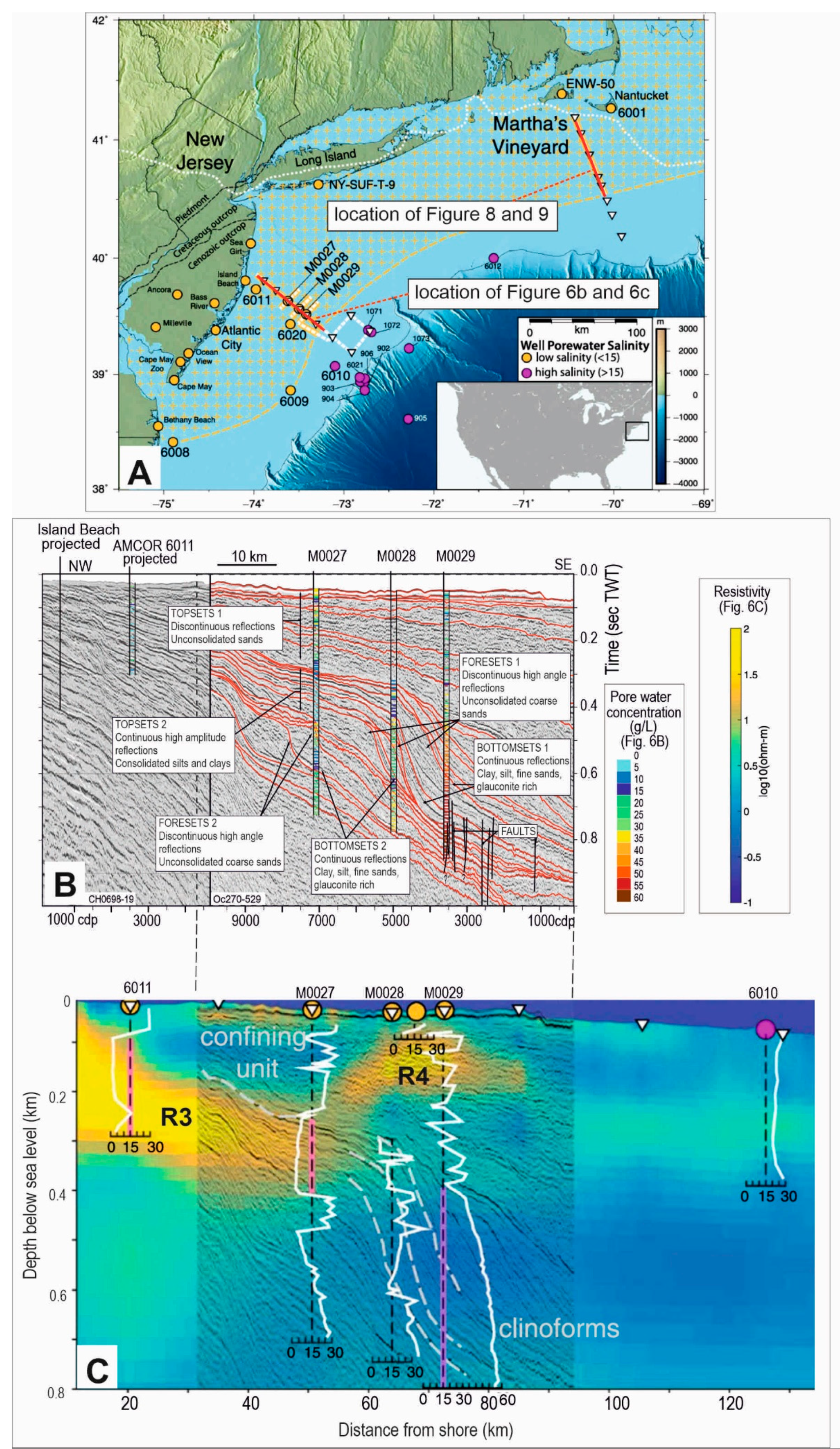
Geological and hydrogeological setting: The sedimentary units of the northern Atlantic passive continental margin (location in Figure 1 and Figure 6) are composed of a wedge of Cretaceous through Pleistocene sediments. The shelf extends 200 km out up to the continental slope (e.g., References [93,94,95,96,97,98,99]. The deepest part of the sedimentary wedge consists of carbonates and minor amounts of evaporites [100]. The upper part consists of a siliciclastic prograding shelf and slope system built since the Oligocene. Beneath the coastal plain, a multilayered aquifer system saturated with low-salinity pore water is prevalently hosted in unconsolidated siliciclastic deposits of Miocene age [6,101,102,103] (Figure 6B). The upper unconfined aquifer locally contains brackish or salty water at the coastline and this saline contamination is due to onshore pumping and salt-water intrusion.
Offshore, beneath the shelf, the presence of pore water (fresher than seawater) is known from a series of boreholes completed during the 1970s and 1980s [92]. The modern onshore hydraulic system is thought to extend offshore, at least beneath the inner shelf where freshwater has been recovered from boreholes in both fine-grained and coarse-grained sediments [92]. Resistivity models derived from shallow water electromagnetic geophysical method support the presence beneath the inner shelf of a low salinity aquifer geometrically connected with the shore and overlain by a low-permeability clay unit acting as a confining unit (Figure 6) [104]. The average porosities of sediments hosting low salinity waters range from 30% to 60% and permeability is estimated between 10 and 1000 mD [17]. The origin of the low salinity groundwater beneath the middle shelf of this area is still debated, with two prevailing hypotheses—first, that it is linked to present-day active dynamic connections with onshore aquifers [19] and second, that it is due to trapped meteoritic and/or sub–ice-sheet waters recharged during lowered sea-level periods [16,92,95,105].
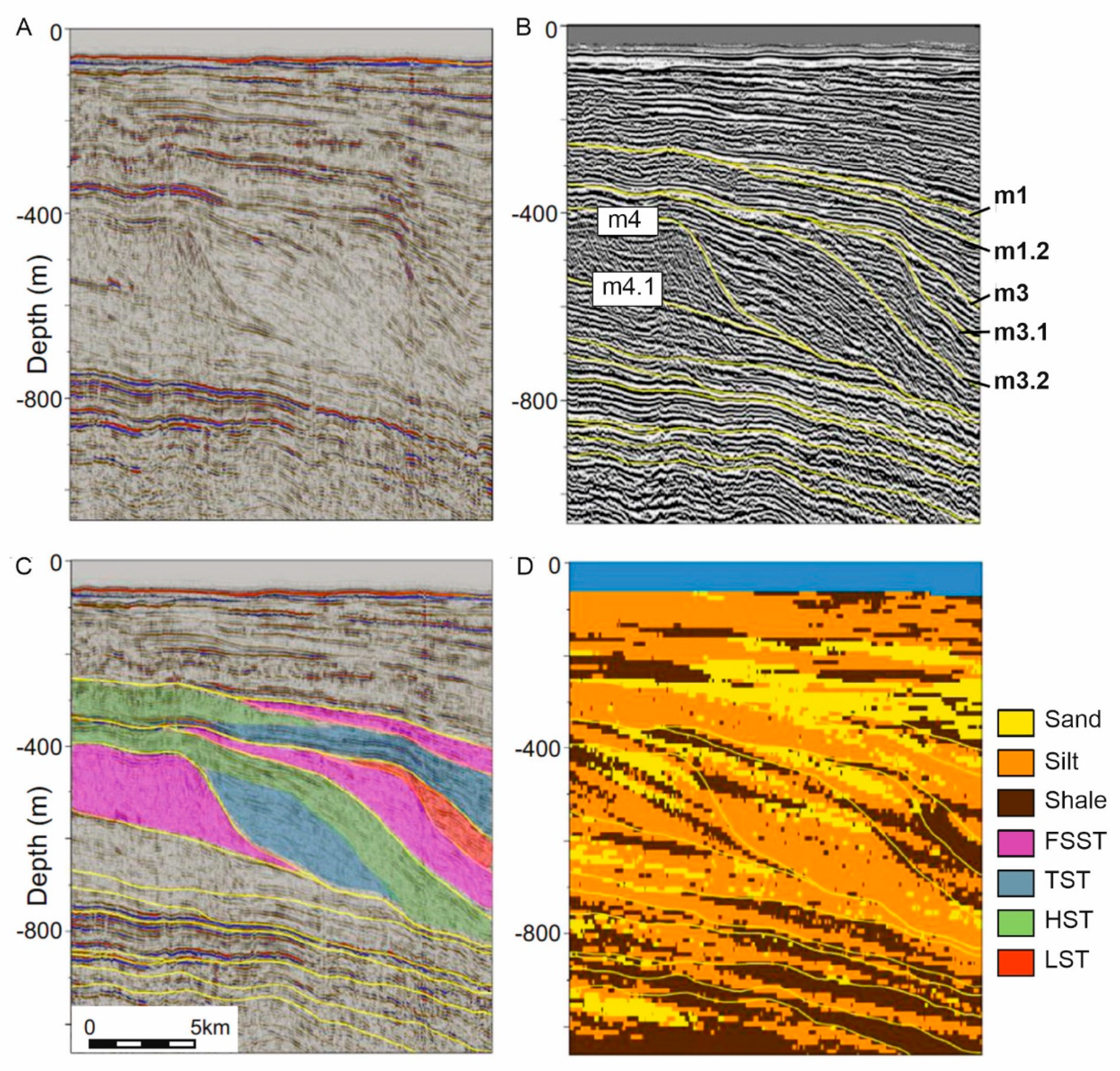
Use of seismic data: The seismic and sequence stratigraphy of this margin is defined in detail with high-resolution chronostratigraphic control (e.g., References [71,106] (Figure 7). Seismic data interpretation shows that pore water salinity is primarily controlled by clinothem geometry, which determines the upwards extent of the low-salinity aquifer beneath the inner shelf (Figure 6B).
Further offshore, in the middle shelf, recent IODP drilling showed that the organization of the offshore reservoirs is also multilayered, with low salinity water (<15 g/L) intervals of different thickness alternating vertically with salty intervals (salinity > 15 g/L) [15]. A direct relationship exists between the sedimentary facies of the siliciclastic system and the salinity distribution of the pore waters, with fresher water preferentially stored in the fine-grained sediments and salty water in coarse grained intervals [17]. Borehole-calibrated seismic data analysis (Figure 6A) shows also that at these sites there is a good correlation between pore water salinity and seismic facies, with the exception of the emplacement of deep upwelling brines [73].
A package of discontinuous seismic reflections corresponds to the recent sand-dominated clinoform topsets, with locally interbedded clay layers and defines the uppermost 200m-thick interval (ca. 0.3 s TWT). This interval hosts alternating salty and fresh pore-waters [17].
The deeper Miocene gently dipping seaward topsets are composed of continuous, high-amplitude reflections that are clay and silt dominated. These deposits preferentially host thick fresh-water intervals (Figure 7). The upper discontinuous to steeply dipping foresets consist of unconsolidated clean sand deposits and preferentially store salty pore-waters. Finally, the lower part of the foresets is dominated by fine-grained deposits which are fresh-water bearing.
The relationship between salinity distribution and seismic facies allowed the development a 2D geometrical model of the reservoir and salinity distribution along a dip section of the shelf margin [17] (Figure 6). In summary, both beneath the inner and middle shelf, fresh water distribution is primarily controlled by clinothem geometry and associated lithology distribution (Figure 7) [17]. However, beneath the inner shelf fresh water is stored in both fine-grained and coarse-grained sediments, whereas beneath the middle shelf, freshened groundwater is preferentially stored in deeper fine grained and low-permeability deposits (clay and silt dominated) and salty waters recovered in coarse-grained deposits (unconsolidated sands). Low permeability barriers such as fine-grained maximum flooding/transgression sediments and cemented diagenetic layers potentially play a role in preserving the emplaced fresh water [17,104,105,107]. Conversely, the faults interpreted in the deeper parts of the seismic sections and based on the results from the resistivity modelling, appear to connect the shallow freshened water aquifers with upwelling fluids from dissolved deep evaporites, facilitating their salinization.
3.1.2. Martha’s Vineyard (Massachusetts)
In this case study (location in Figure 1 and Figure 6) seismic methods have been used to understand reservoir properties, aquifer onshore-offshore connectivity and paleo-coastline definition, in a siliciclastic, passive margin setting.
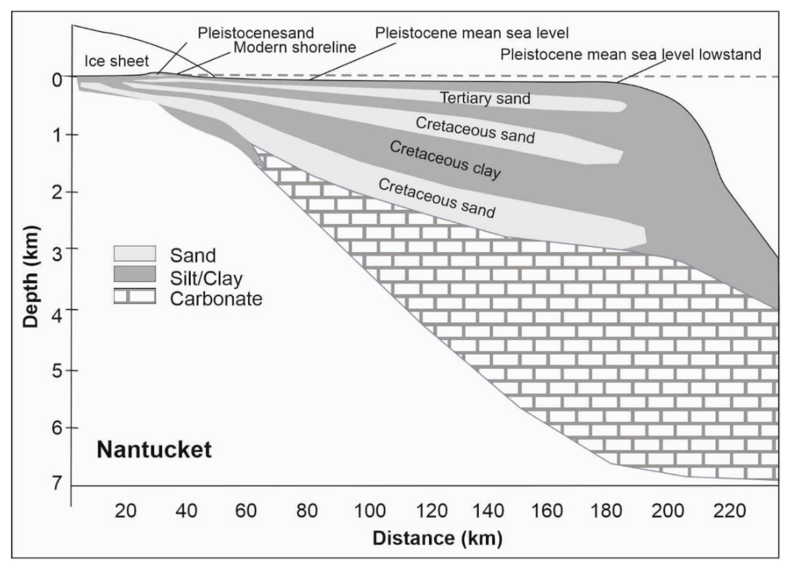
Geological and hydrogeological setting: The hydrogeology of the continental-shelf sedimentary units beneath Nantucket Island and offshore into Martha’s Vineyard, present many analogies with the case study of New Jersey [95,96,108,109,110,111,112] (location in Figure 1 and Figure 6). The stratigraphic and hydrostratigraphic units span the Cretaceous to the Holocene (Figure 7) and show significant variability in thickness downdip and along strike. On Nantucket Island, freshwater extends to depths greater than 500 m below sea level [93,113].
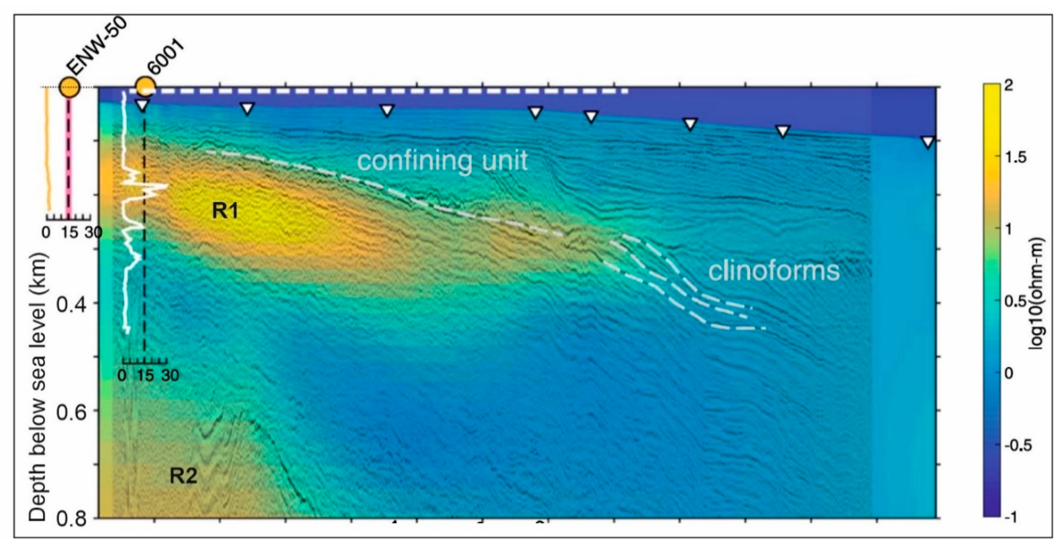
A 514-m-deep borehole (USGS 6001, from Reference [47]) (location in Figure 6A) penetrating the entire Cretaceous sedimentary package and two shallower wells (100 m), completed in the Miocene–Pleistocene sands, all had pore-water salinities of less than 1 ppt within the permeable intervals. The relatively thick clay and silt layers in well USGS 6001 exhibited higher salinity levels (30–70% seawater) and displayed a geometry consistent with ongoing vertical diffusion. The permeability measured on Nantucket Island in low-salinity aquifers range from 10–780 mD and it allows flow of water through sediments [98,107]. The exact extent of the low-salinity groundwater offshore Massachusetts isis unknown, as no offshore drilling has confirmed the predicted models.
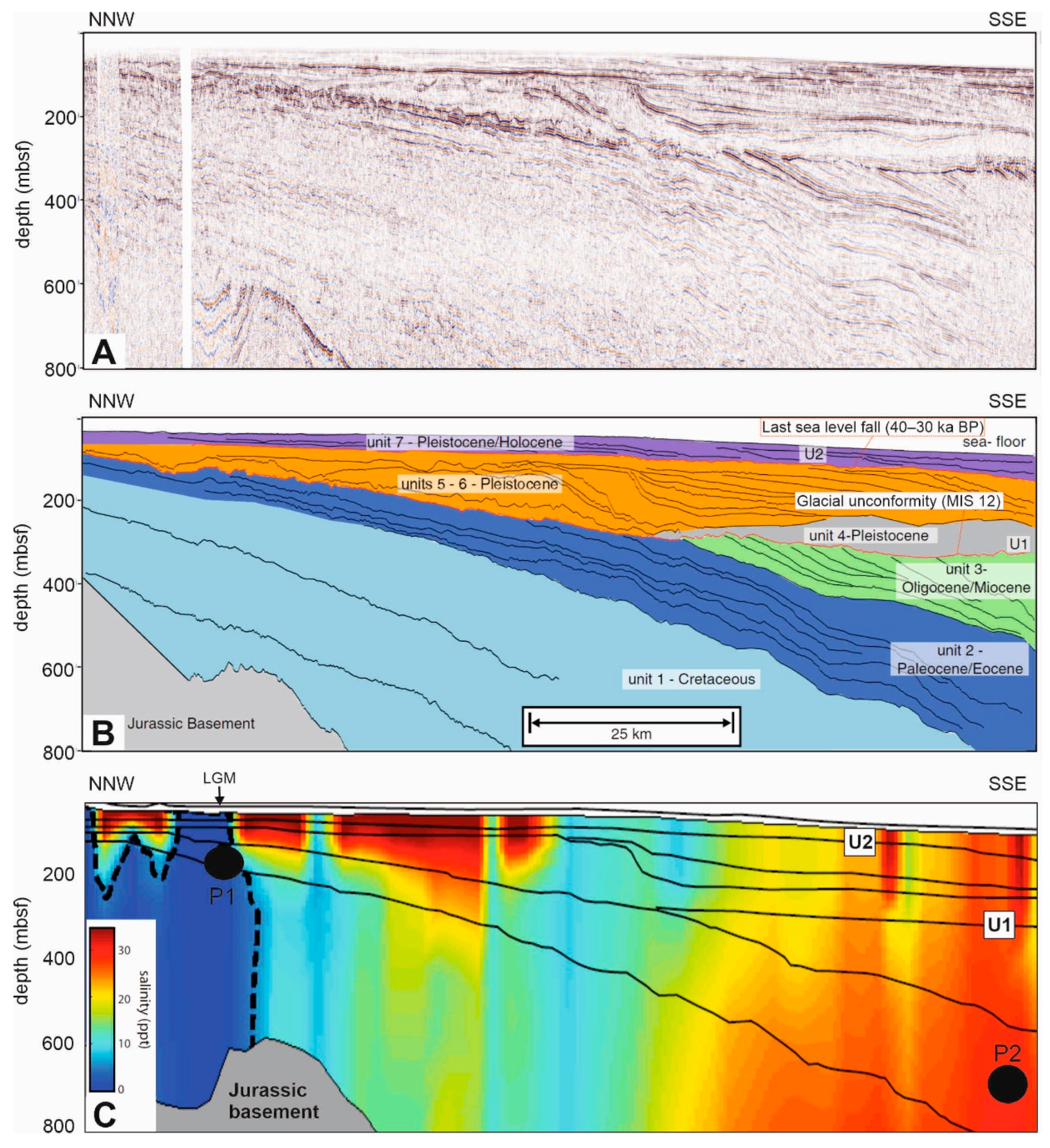
Use of seismic data: Recent studies [117,118] use high-resolution, multichannel 2D seismic data to define the stratigraphy and constrain a three-dimensional, variable-density model that couples fluid flow, heat and solute transport for the continental shelf (Figure 9). Clastic Oligo-Miocene units are separated from the overlying Pleistocene-Holocene units by a prominent glacial unconformity (U1 in Figure 8), interpreted as marine oxygen isotope stage (MIS) 12 [119]. U2 (Figure 8) is a shallow sequence boundary that formed during the last sea level fall (40–30 ka B.P.) and marks the onset of siliciclastic sedimentation and glacial outwash during the late Pleistocene and Holocene [117,120]. According to the authors, freshwater distribution on this margin is strongly dependent on depositional architecture and ice sheet history. Model results indicate that the late Pleistocene ice sheet was responsible for much of the emplaced freshwater. Through seismic data analysis the authors are able to estimate the maximum extent of the late Pleistocene ice sheet to near the shelf-slope break (U2 in Figure 8).
Similarly to the New Jersey case study, seismic reflection images co-rendered on resistivity models (Figure 9) reveal consistent architectural controls on the low-salinity groundwater distribution [104]. Continuous, well-defined stratigraphic boundaries mark the upward extent of low-salinity groundwater and the onset of Oligo-Miocene clinothem deposition is thought to limit the seaward extent of the resistive bodies that are interpreted as fresh-water bearing. The authors suggest that the resistive body R1 (freshwater aquifer) (Figure 10) connects onshore, as shown by comparison with the well ENW-50 and is thus consistent with seaward transport of freshwater from onshore recharge through coarse sediments.
3.1.3. Florida
In this case study, seismic methods have been used for characterization of reservoir properties, aquifer onshore-offshore connectivity, paleo-continental environments, identification of dissolution-related karstic features and associated fossil aquifers.
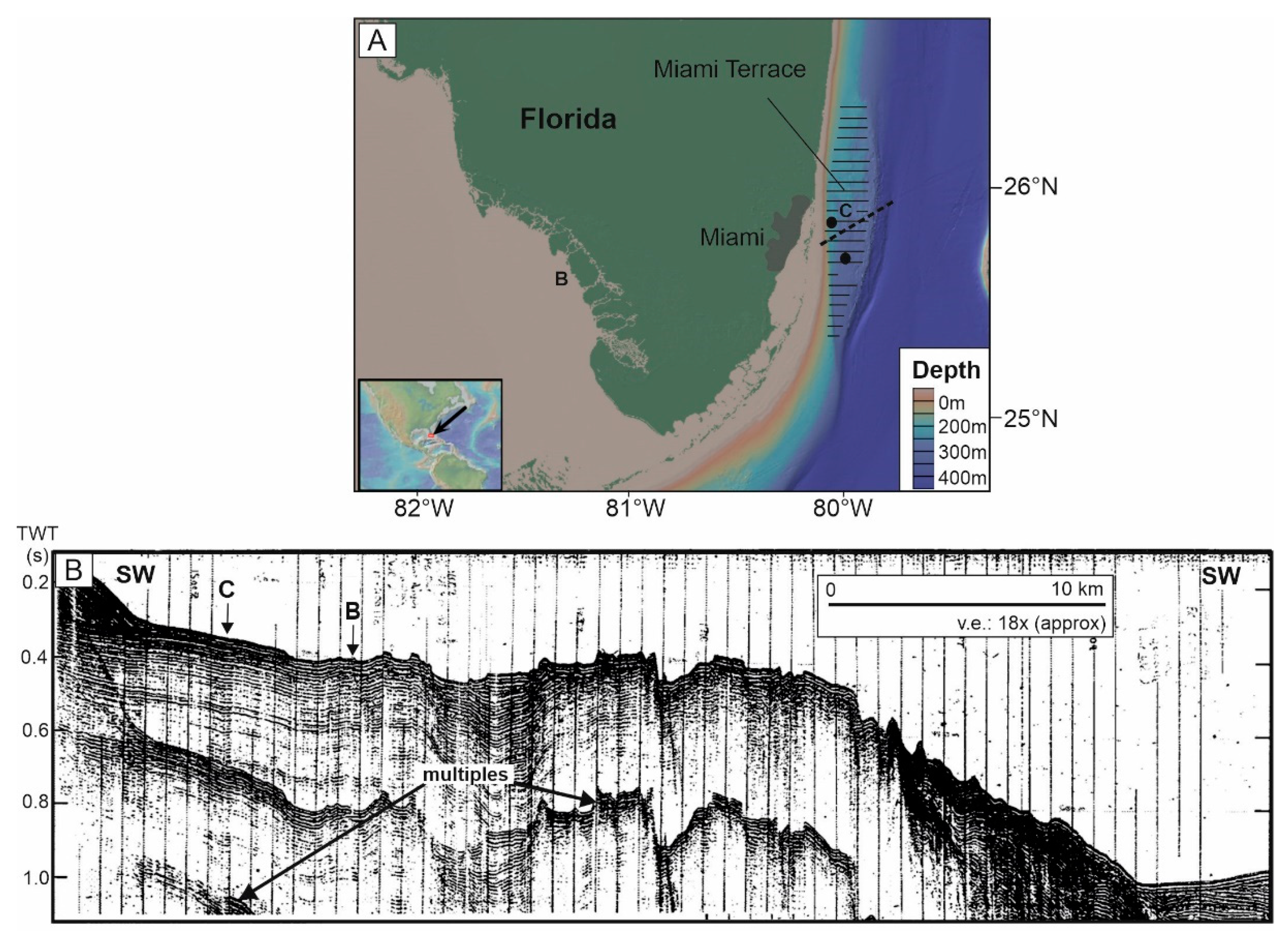
Geological and hydrogeological setting: The Floridan Plateau is a broad, flat limestone and dolomite platform separating the Atlantic Ocean from the Gulf of Mexico [121] (Figure 10). This Plateau hosts the Floridan aquifer, one of the most productive aquifer systems worldwide (Figure 10). In northeastern Florida, water within this aquifer system can be under artesian pressure, depending on the permeability of overlying strata [122,123,124]. The aquifer can be subdivided into two moderately high permeability systems, referred to as the Upper and Lower Floridan. A series of relatively impermeable Miocene and younger beds confine the aquifer. The continental shelf is about 110-km wide [125] and a large volume of freshened groundwater under artesian pressure is known to exist beneath the Atlantic Ocean [100,126]. A geologic exploratory well drilled 43 km offshore from Jacksonville penetrated an artesian aquifer at 250 m depth below sea level. Historic submarine discharge has been observed to occur off the coast of Florida [121,127], with active springs, located a few kilometers offshore, associated fractures and sinkholes ([122] and references therein).
Use of seismic data: Seismic data have been used in this region both to identify karstic vents on the seafloor and karstic morphology in the subsurface. A fresh water discharge vent is visible on seismic profiles, close to an ancient collapse feature (Figure 4A) [77]. In the Straits of Florida, in the southern part of the case study area, detailed bathymetric and high-resolution seismic records reveal well-defined karstic morphology and multiple large collapse features on the Miami and Poutales Terraces, currently located at 200–400 m water depth and at 10 s to 100 km from the coastline ([75], Figure 10). These features are linked to sustained submarine discharge of artesian water [75,81] (see also Section 2.2).
The submarine karst morphologies and the narrow and linear distribution of sinkholes on the two terraces may indicate the past or present location of mixing zones, where limestone dissolution and solution-collapse processes are enhanced [75]. The formation of some of the sinkholes observed in the Straits of Florida has been related to late Miocene-Pleistocene sea-level lowstands resulting in an elevated head and stimulating artesian flow of groundwater out of the aquifer [128,129].
Subaqueous formation of sinkholes in the same region is also associated with submarine discharge of fresh groundwater flowing from the nearby platform [81] (Figure 10). These sinkholes are located on the seabed at water depths greater than 600 m, which is deeper than any Neogene eustatic change [124]. Glacial sea-level lowstands during the Pleistocene would have presumably stimulated submarine artesian flow in the area and caused the sinkhole formation, with only a 10 m increase in head within the onshore Floridan aquifer [81].
3.2. Mediterranean Region
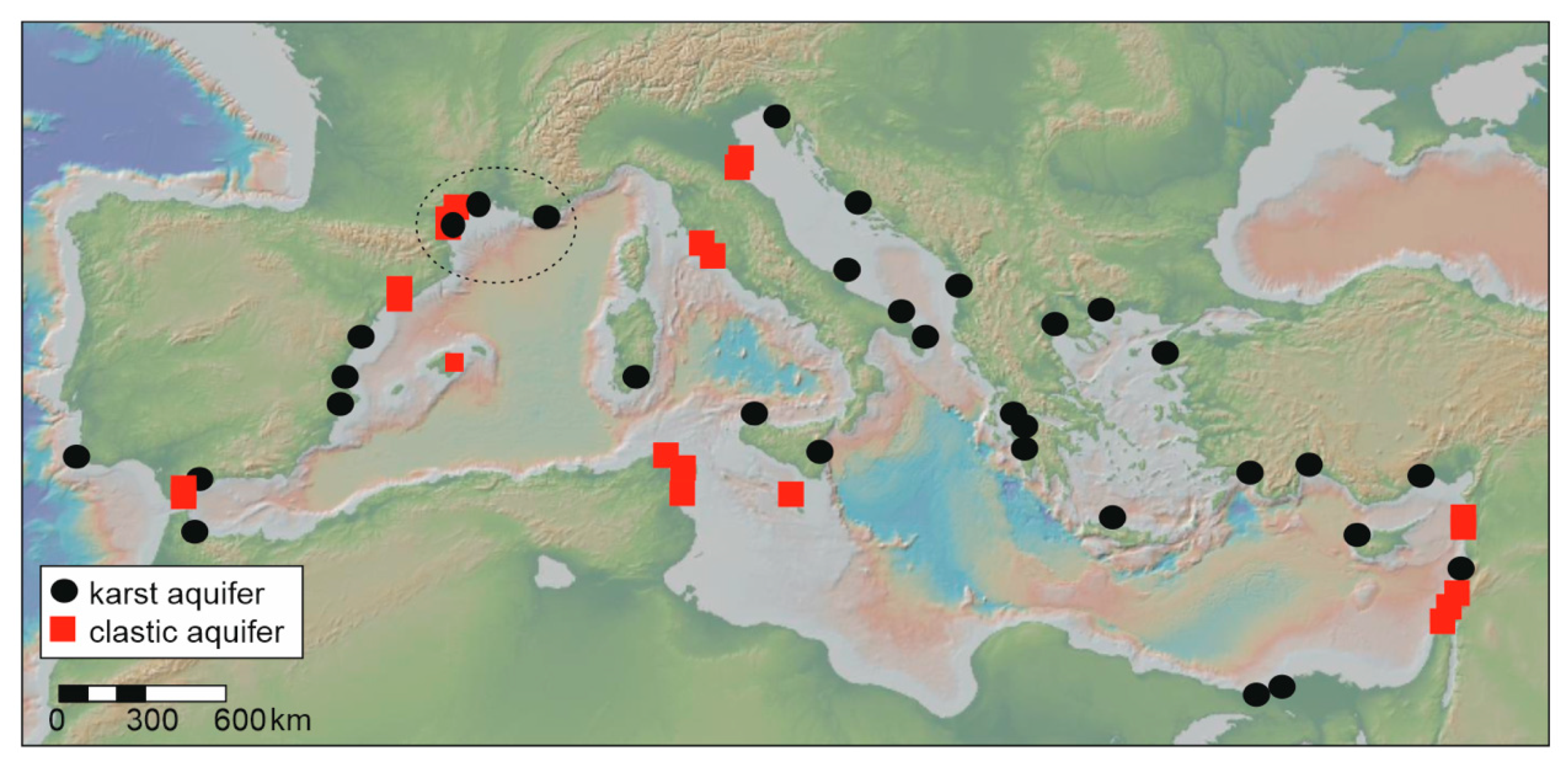
The Mediterranean region (Figure 11) offers a series of examples of coastal aquifers and their shallow offshore extension, in both karstic and clastic (carbonate and terrigenous) sediments. We show a case study in Southern France, where seismic data derived from both academia (shallow penetration, high resolution) and oil and gas industry (deeper penetration, lower resolution) have been used for reservoir architecture and characterization, pending ground-truthing from borehole sampling.
Geological and hydrogeological setting: The majority of Mediterranean coastal porous aquifers are hosted in clastic sediments and are located in Pliocene to Quaternary deposits [9,132,133,134,135]. These aquifers are “coastal detritic formations” following the classification for European aquifers by Reference [136] (Figure 12). They are often multi-layered and mainly studied onshore. As littoral zones are important places of economic development, they are often linked to intensive water needs for agriculture, drinking water supply, tourism and industry. These aquifers are extremely sensitive to sea-level and climatic changes, due to the Mediterranean Sea configuration as a landlocked basin (e.g., Reference [137]). As a consequence of these factors and of over-exploitation, the quality of coastal aquifers in the region is currently heavily affected by seawater intrusion (Figure 11) [2,138]. Seawater intrusion at shallow depth can also occur naturally as a result of offshore strata geometries (Figure 12A).
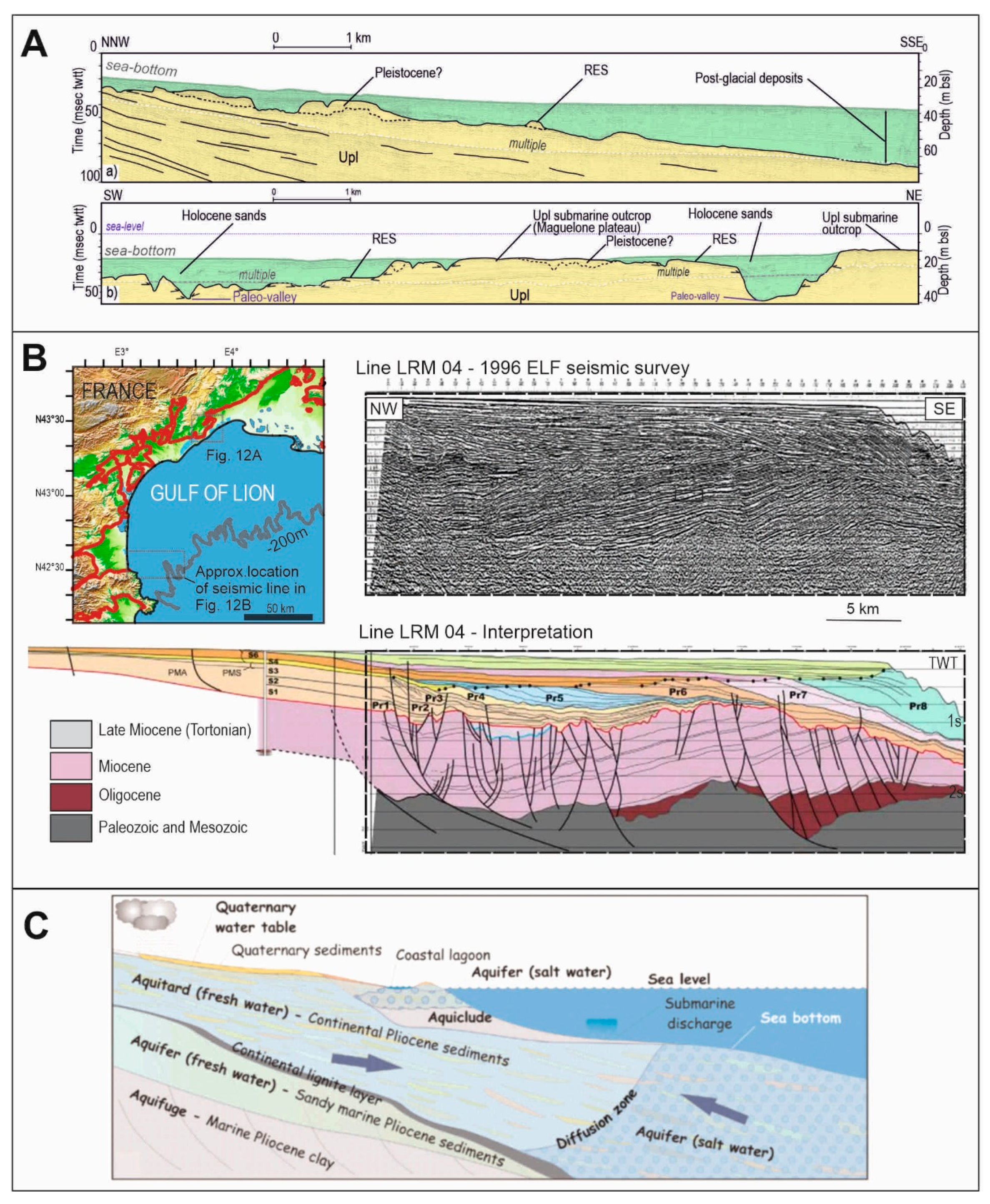
In Southern France, the Plio-Quaternary calcareous sands are one of the most important aquifers for the freshwater supplies in the Gulf of Lions coastal areas, such as the complex multi-layered aquifer located below the Roussillon coastal plain and potentially extending into the offshore (Figure 12). This aquifer is hosted in marine and continental Pliocene and Quaternary coarse grained sediments. Each aquifer layer is characterized by different hydrogeological properties [132]. Geochemical and isotopic analyses performed on groundwater samples taken from two coastal boreholes [135] showed groundwater residence ranging from about 15 ky in the deep Pliocene aquifer to 5 ky in the intermediate Pliocene aquifer [135].
Use of seismic data: The extent of coastal aquifers into the offshore clastic Plio-Pleistocene shelfal reservoirs has been mapped using high-resolution, shallow seismic and deep, lower resolution industry data, tied to onshore boreholes [73] (Figure 12). The offshore record mostly consists of prograding clinothems. As for the New Jersey margin case study, beneath the coastal plain, a multilayered aquifer system saturated with fresh pore water is hosted in unconsolidated siliciclastic sediments. The upper part may locally contain brackish or salty water at the coastline. The present day extent of the low-salinity groundwater beneath the shelf is currently uncalibrated. However due to the similarity in geological setting and hydrogeological conditions with the New Jersey shelf, it can be inferred that fresh water distribution might be primarily controlled by clinothem geometry and associated lithology distribution.
3.3. East Africa
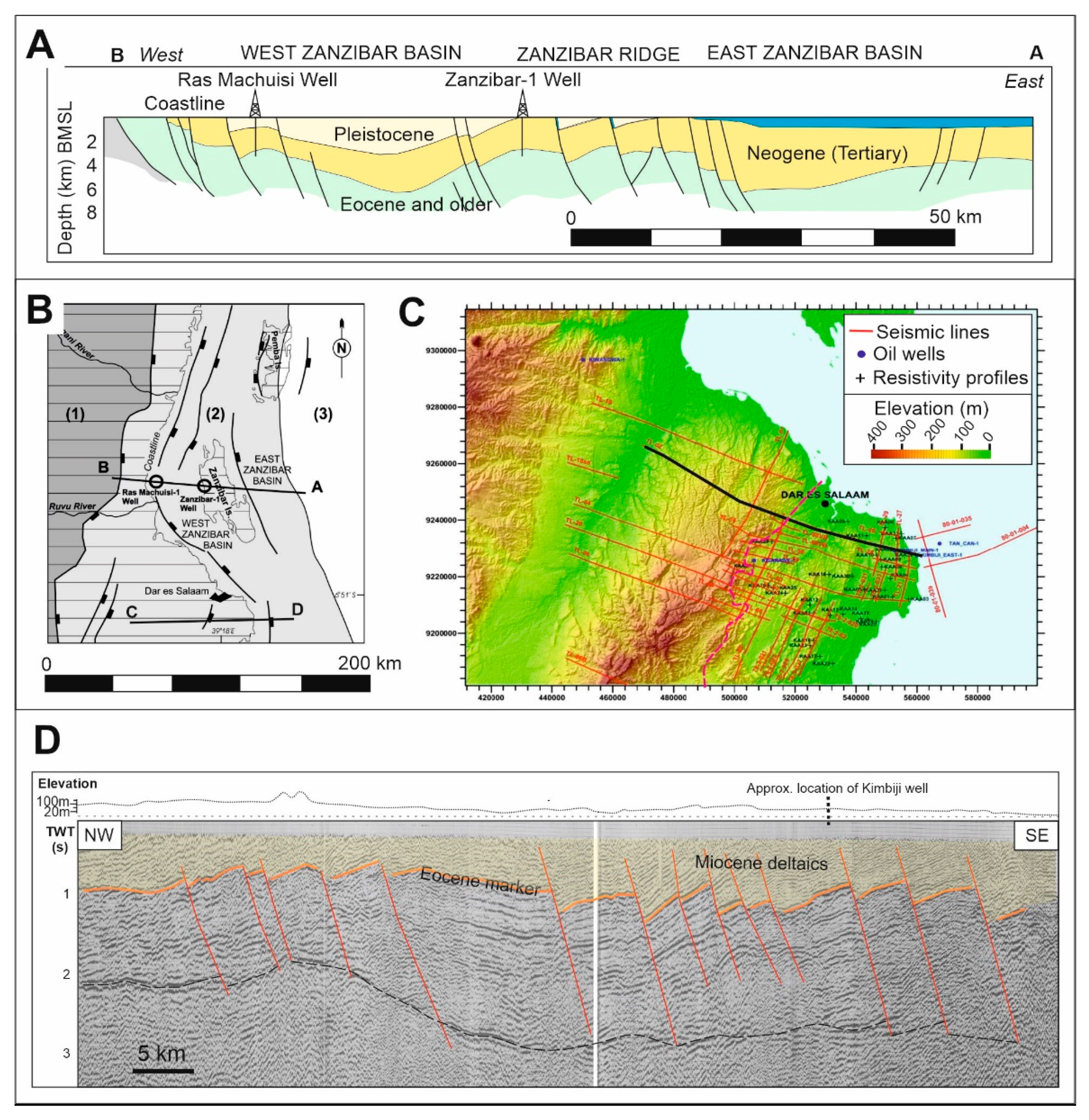
This case study demonstrates the use and value of oil & gas exploration data for deep groundwater exploration purposes in a coastal setting in Tanzania. Models obtained from seismic reflection data were used to define the geometry and reservoir architecture of a deep coastal aquifer system (the Kimbiji Aquifer) near the city of Dar es Salaam [139,140]. The geological model of the Kimbiji Aquifer is verified by drilling, both onshore and in the shallow offshore. The hydrogeological model is verified by drilling and testing activity onshore and is guided offshore by established hydrogeological principles and numerical groundwater modelling techniques.
Geological and hydrogeological setting: The Kimbiji Aquifer comprises a thick sequence of paleo-deltaic sediments of mainly Miocene age [20,139,140,141] overlying Lower Tertiary carbonates (Figure 13). The sediments, which are associated with a rapidly subsiding basin, are layered and heterogeneous in nature and incorporate sands, gravels, clays and marls.
Seismic reflection profiles show how the stratigraphic sequence hosting the Kimbiji Aquifer onshore extends in the offshore domain, where it thickens beneath the Indian Ocean. At the coastline, the verified thickness is 1.5 km [140].
The complex, layered aquifer system becomes increasingly confined with depth. Deep artesian heads were encountered in several exploration wells, both near the coast and on structurally elevated positions within the Kimbiji Aquifer. Onshore drilling campaigns in 2006–2007 and 2013–2017 demonstrated that high-yielding production wells can be developed, abstracting low-salinity groundwater of potable quality. The apparent age of groundwater that was pumped from depths of 600 m was approximately 40,000 y, which is consistent with simulated flow velocities using a regional numerical groundwater model.
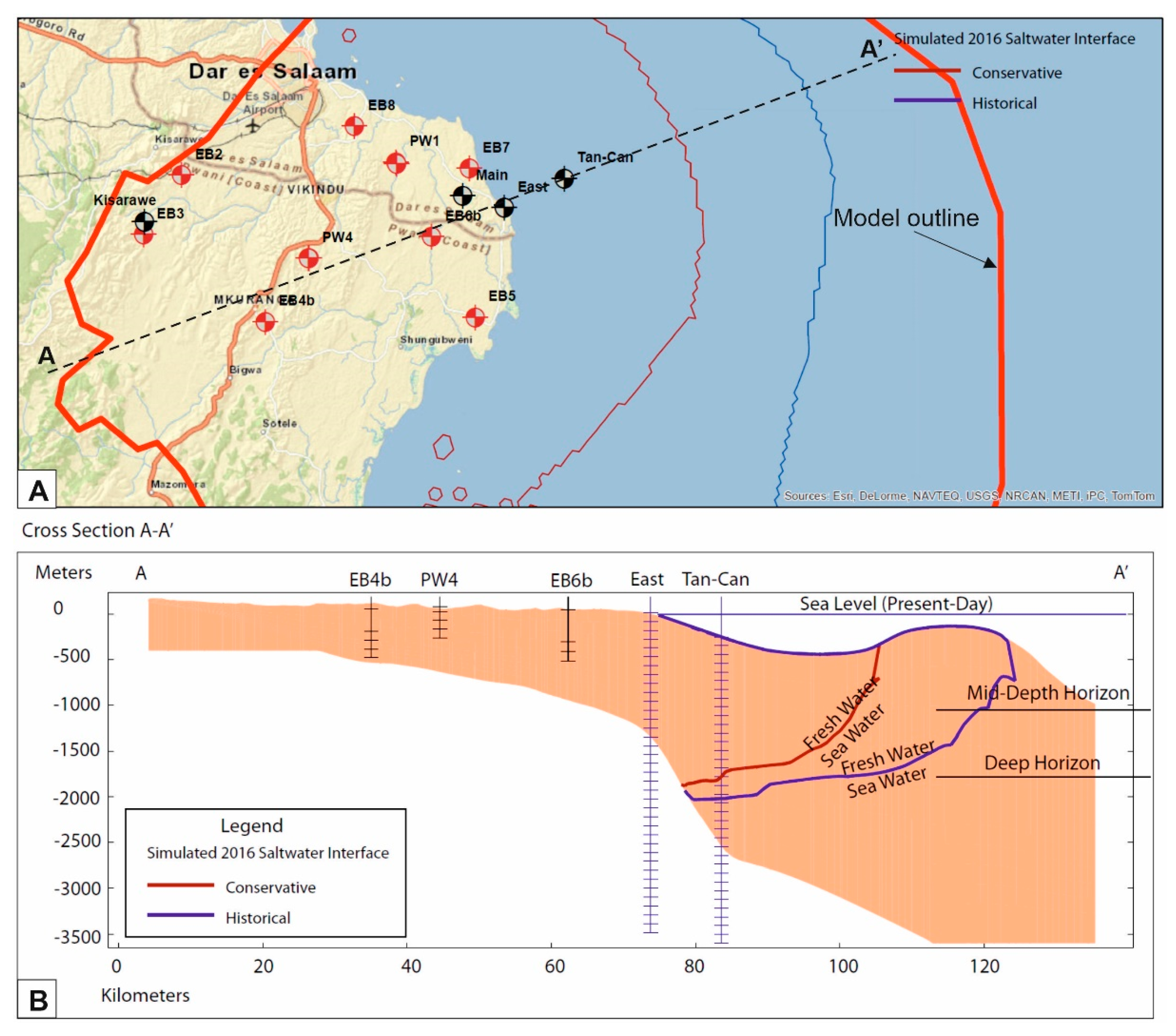
Numerical groundwater modelling also indicates that large-scale abstraction of up to 200,000 m3/d may be sustained without inducing saline intrusion for a period of 100 years [140]. Under a hydrogeological scenario that is defined by current, measured groundwater and seawater levels, the simulated fresh-saline groundwater interface extends approximately 25 km offshore (Figure 14). Under a different scenario which accounts for the deeper seawater levels that prevailed during the Pleistocene and Holocene [142,143], a 19,000-year simulation of subsequent sea level rise simulated an interface which extends approximately 40 km offshore (Figure 14). Thus, a significant volume of fresh groundwater is inferred to extend a significant distance offshore.
Extending east from Dar es Salaam and the Kimbiji Aquifer region, the area between coastal mainland Tanzania and the island of Unguja (Zanzibar) is characterized by basin thicknesses up to 6000 m of Neogene/Pleistocene/Holocene sands (Figure 13). The basin axis is oriented roughly N-S, with a water depth rarely exceeding 40 m and with a total basin thickness exceeding 10,000 m in places. Logs from hydrocarbon exploration wells in the West Zanzibar Basin indicate bulk resistivity values in sand sequences pointing to the potential presence of fresh water [141].
Use of seismic data: Hydrocarbon exploration data are not conventionally or traditionally used in water exploration activity. In the case of the Kimbiji Aquifer, both the discovery [139] and study phase of the aquifer system [140] relied on access to oil & gas exploration data. The seismic reflection data, especially, was instrumental in defining the scale and magnitude of the aquifer system and its possible connection with deeper geological formations. The interpretation of the seismic data were aided by oil & gas well completion records, which included both geological and wireline logs, as well as drill stem test data.
In the case of the Kimbiji Aquifer study, the access to 1140 km of seismic data was facilitated by the Dar es Salaam Water and Sewerage Authority under an agreement with the Tanzanian Petroleum Development Corporation. The data that could be accessed was from the early 1980s and although data and record formats were of variable nature and quality, careful review and analysis allowed older records to be ‘recycled’ for water exploration purposes.
3.4. Canterbury Bight, New Zealand
In this case study, shallow penetration and high resolution seismic data have been used for reservoir characterization and identification of faults and buried valleys in a siliciclastic passive margin setting.
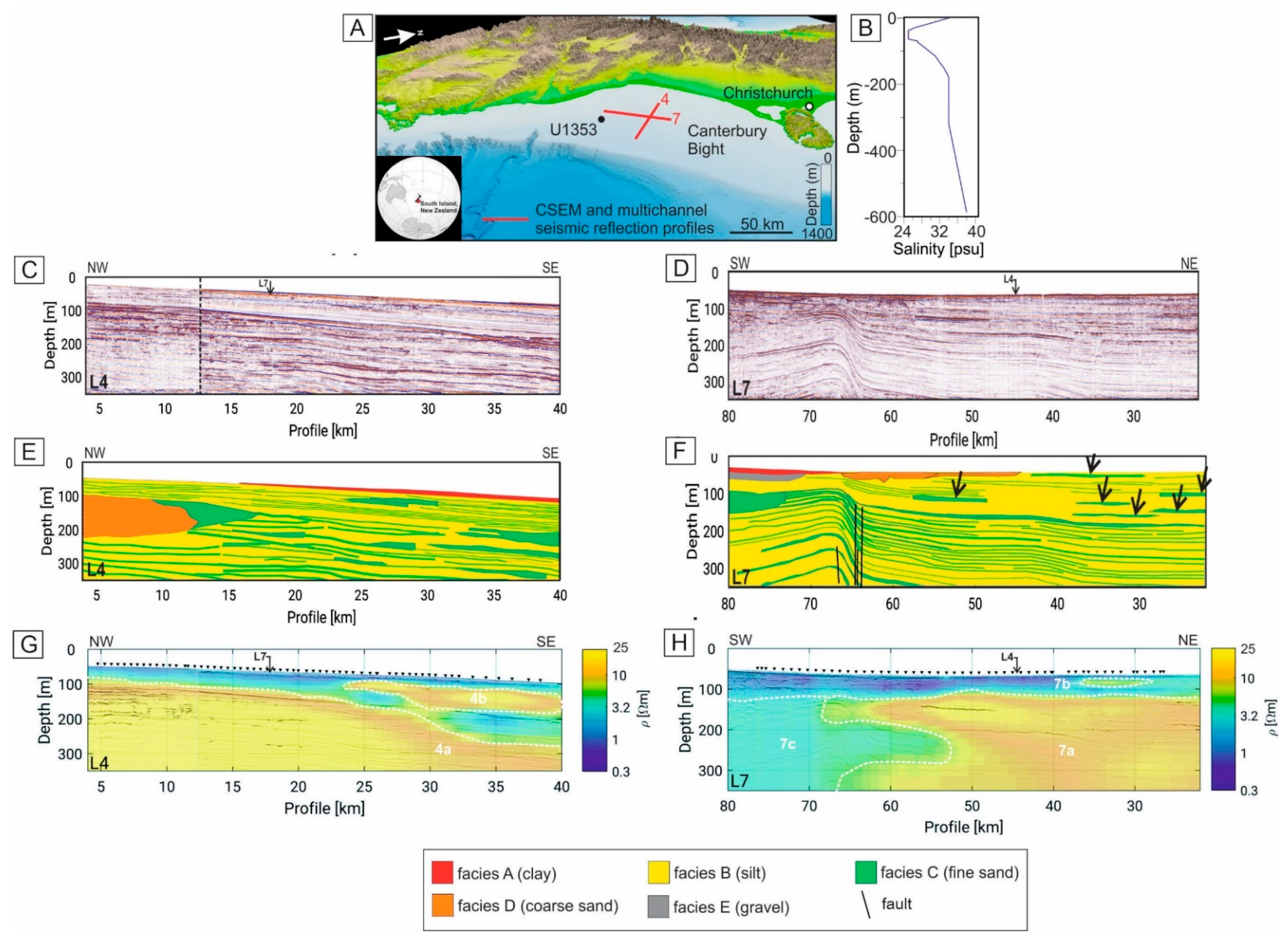
Geological and hydrogeological background: An offshore freshened groundwater system hosted in unconsolidated, clastic sediments has been reported in the Canterbury Bight (located off the eastern coast of the South Island of New Zealand) [31] (location in Figure 1; Figure 15). The Canterbury Bight is a 95 km wide and up to 140–150 m deep continental shelf. It comprises a 1 km thick progradational succession of shelf-slope deposits punctuated by advances of the braid plain during periods of sea level fall [145]. Eustatically-driven transgressive-regressive cycles have controlled the sedimentary history of the Canterbury Bight since the middle Miocene [146,147,148].
Use of seismic data: Seismic reflection profiles across the Canterbury Bight were divided into five different facies using multi-attribute seismic facies classification (Figure 15C–F). The latter entailed two steps: (i) sub-division based on amplitude characteristics, lateral continuity, reflector geometry and two seismic attributes-instantaneous frequency and envelope [149]; (ii) determination of a depth–travel time relationship from the sonic logs and correlation of the features in the borehole logs, recorded in the depth domain, with those in the seismic reflection data, recorded in the time domain; a synthetic seismogram was constructed in the boreholes from the sonic log and the density curve was calculated from the resistivity log using Archie’s relationship [150]. Four of the five facies (clay, silt, fine sand and coarse sand) could be correlated with lithologies in the boreholes, whereas the fifth one was interpreted as gravel in view of the similarity of the seismic facies with that of gravel onshore.
The stratigraphic framework that emerges from the classification of the seismic reflection profiles is an alternation of lowstand fluvial gravels and sands, which become thicker towards the shore and highstand sands, silts and clays, which are more dominant in the deeper sections. This distribution of facies is consistent with that of sediment transport models [145].
The CSEM resistivity data, locally calibrated by pore water salinity measurements from boreholes, point to an offshore groundwater system that consists of one main and two smaller, low salinity groundwater bodies (Figure 15G,H). The main body has a maximum thickness of at least 250 m and extends up to 60 km from the coast and a seawater depth of 110 m. The maximum groundwater volume estimated from the CSEM resistivity data for a porosity of 40% is 213 km3.
The offshore freshened groundwater occurs in sedimentary layers that mainly include silt and sand and occasionally gravel and clay. More importantly, a recent study [31] reports a spatial variability in groundwater salinity along the shelf. This can be attributed to specific sedimentary structures (e.g., high permeability conduits and corridors; the latter are visible as 5–10 km long isolated bodies of parallel, continuous, high amplitude reflectors occurring at multiple depths and interpreted as buried valleys) and normal faults primarily acting as barriers and potentially to recharge from rivers during sea level lowstands.
A meteoric origin of the offshore freshened groundwater and active migration from onshore are inferred based on the geochemical characteristics of the pore water in the borehole data and the recent groundwater age at the coast. However, 2D models of groundwater flow and solute transport, based on the interpretation of the seismic reflection profiles, indicate that recharge from onshore aquifers can only account for a small fraction of the offshore freshened groundwater at present. The majority of the offshore freshened groundwater was emplaced during the last three glacial cycles. Topographically-driven shore-normal flow was higher than at present during sea level lowstands, due to an increase in the hydraulic head and steep onshore gradients. Such flow was reduced during sea level highstands, when lateral differences in salinity on the shelf drove groundwater laterally or shoreward.
3.5. Gippsland Basin, Australia
In this case study, seismic data provided the framework for the characterization of aquifer/reservoir architecture, mapping of regional hydrostratigraphic units at a basinal scale and their onshore-offshore connectivity, in a mixed carbonatic-siliciclastic setting.
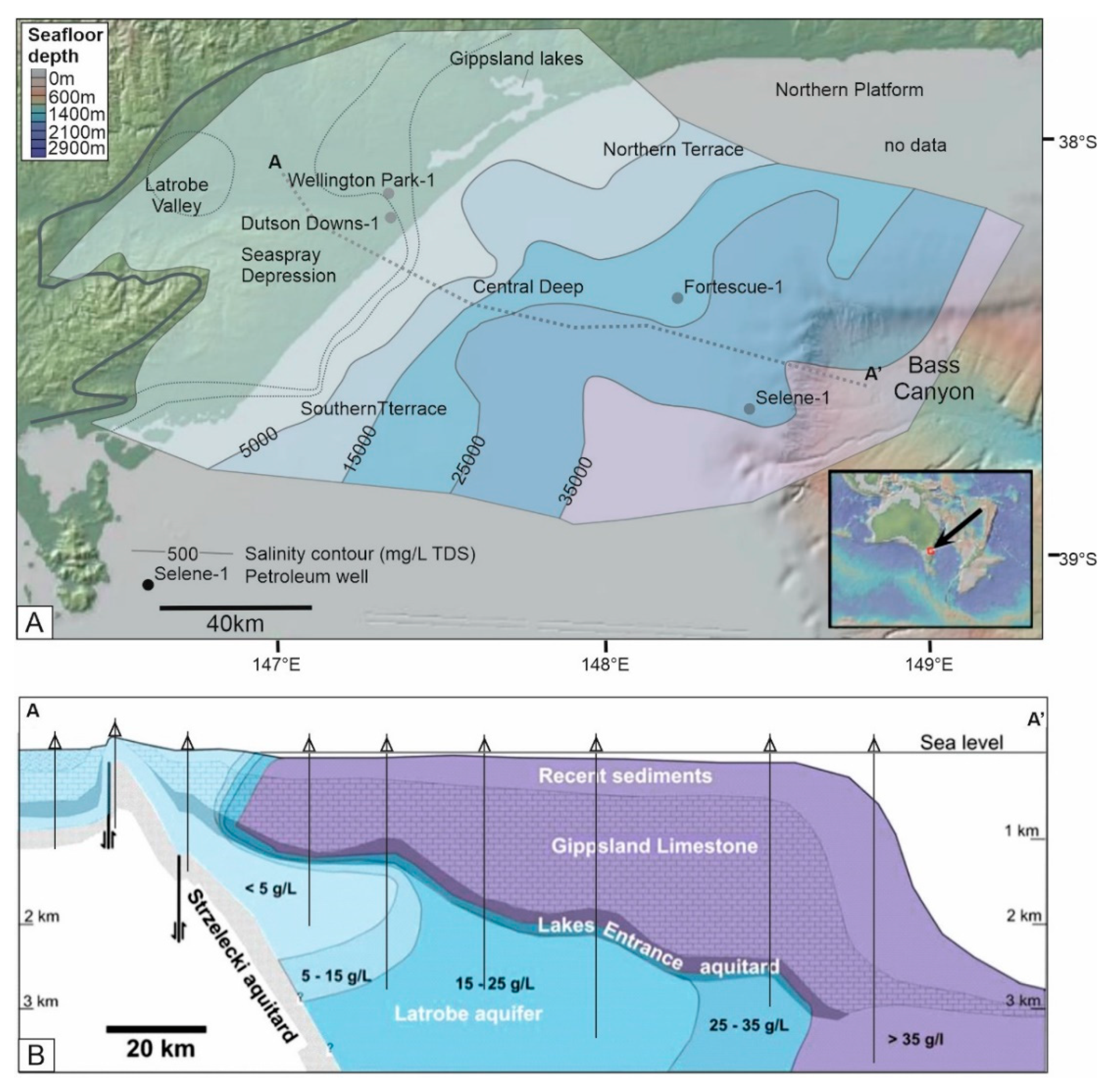
Geological and hydrogeological background: Evidence of aquifers connected to onshore groundwater have been found offshore southern Australia [151,152] (Figure 16, general location in Figure 1), through the use of combined seismic data, onshore and offshore wells, historical production and pressure data. Data have been acquired through the years in successive campaigns focused on oil and gas exploration and the mining industry. This case study thus offers an example of a multiple usage aquifer and the consequences of its exploitation—significant withdrawal of fluid resulted in a complex pattern of pressure decline in the aquifer, potentially associated with its usage [153].
The basin extends from onshore to offshore and hosts depositional sequences ranging in age from Early Cretaceous to Holocene. The main deep aquifer is hosted in the Latrobe Group sediments, of Cretaceous to Oligocene age, composed of siliciclastic sediments, ranging from alluvio-fluvial sediments at the base to marginal-marine, deltaic and increasingly marine sediments, sealed by the confining aquitard of the Lake Entrance formation (marine shales of late Oligocene age) and by the Strzelecky aquitard below (sandstones and shales of Albian age) (Figure 16) [151,152,154]. The Latrobe Group forms a major freshwater aquifer (Latrobe aquifer) in the onshore part of the basin. This sedimentary unit also contains substantial coal resources that are being mined in the onshore part of the basin [151].
Use of seismic data: Approximately two thirds of the basin are located offshore. The Latrobe group has been identified as the most important reservoir for oil and gas in both onshore and offshore parts of the basin. Seismic data have been used to reconstruct stratigraphic cross sections and define the vertical and lateral extent of the Latrobe reservoir/aquifer and the various hydrostratigraphic units in the offshore.
The salinity of the formation water in the Latrobe aquifer varies from less than 0.5 g/L in the onshore area to more than 30 g/L total dissolved solids (TDS) in the Central Deep region of the offshore Gippsland Basin. In the deep Latrobe aquifer a lower salinity gradient and wide zone of brackish formation water extends to about 20 km offshore. Based on both wells and seismic data, the freshwater hydraulic-head distributions and the architecture of the sedimentary units suggest that groundwater flows from the northern and western margins towards the central part of the basin. Freshwater hydraulic heads in the western part of the basin imply that there is a source of water in the Central Deep where the Latrobe Aquifer occurs at depths > 2500 m below sea level and subcrops beneath the seafloor.
4. Discussion and Conclusions
4.1. Summary of Use and Limitations of Seismic Reflection Data in Offshore Freshened Water Research
The selected case studies highlight how seismic data has been used, indirectly, in the identification and mapping of geological features hosting aquifers in the offshore realm. Seismic data is an important tool in a workflow that includes other geophysical and geological methods (see Section 1.2), in order to understand the quality (salinity) of offshore groundwater. In this context, lower resolution, deep penetration seismic data would be applied, initially, in an exploratory and scouting phase, with higher resolution and shallow penetration data subsequently applied to define the details of shallow aquifers and their geometry in any prospective area. Therefore, existing deeper penetration industry data can be used to widen the search for offshore freshened groundwater in a global context, if implemented by additional data and techniques.
So far, in the described examples and other case studies worldwide, seismic stratigraphic and sequence stratigraphic interpretation has predominantly provided value for the analysis of (Figure 17):
- Reservoir (aquifer) properties and architecture, for example, through spatial mapping of the permeability/porosity of sedimentary bodies, analysis of onshore-offshore aquifer connectivity, identification of the open or confined nature of offshore aquifers and their active or ‘fossil’ setting. In carbonate rocks, seismic data can also indicate areas of porosity and permeability enhancement due to karstification processes (Section 3.1, Section 3.2, Section 3.3, Section 3.4 and Section 3.5)
- Seal (aquitard/aquiclude), through the identification of permeability barriers, such as laterally extensive fine-grained sediments or tightly cemented layers (Section 3.1.1)
- Paleo-continental environments, through the detection of potential freshwater-bearing environments, such as fluvio-lacustrine systems or subaerially exposed karstic terranes (Section 3.1.3),
- Paleo-coastline and change to active aquifers: absolute and relative sea-level changes and shift of coastal facies through time and therefore potentially associated coastal aquifers (e.g., References [44,67]); The onlap shifts related to sea-level change are used to document shifting of the mixing zone and saltwater intrusion into coastal plain groundwater systems in the past (Section 3.1.2)
- Conduits, (paleo)channels and canyons, faults as conduits or indication of fractured reservoirs, sinkholes, pockmarks/pipes. Faults can alternatively act as barriers when juxtaposing the reservoir to sealing units. (Section 3.1.1, Section 3.1.3, Section 3.3 and Section 3.4)
- Aquifer indicators, subaerial sinkholes and other dissolution-related karstic features, pockmarks/pipes (Section 3.1.3)
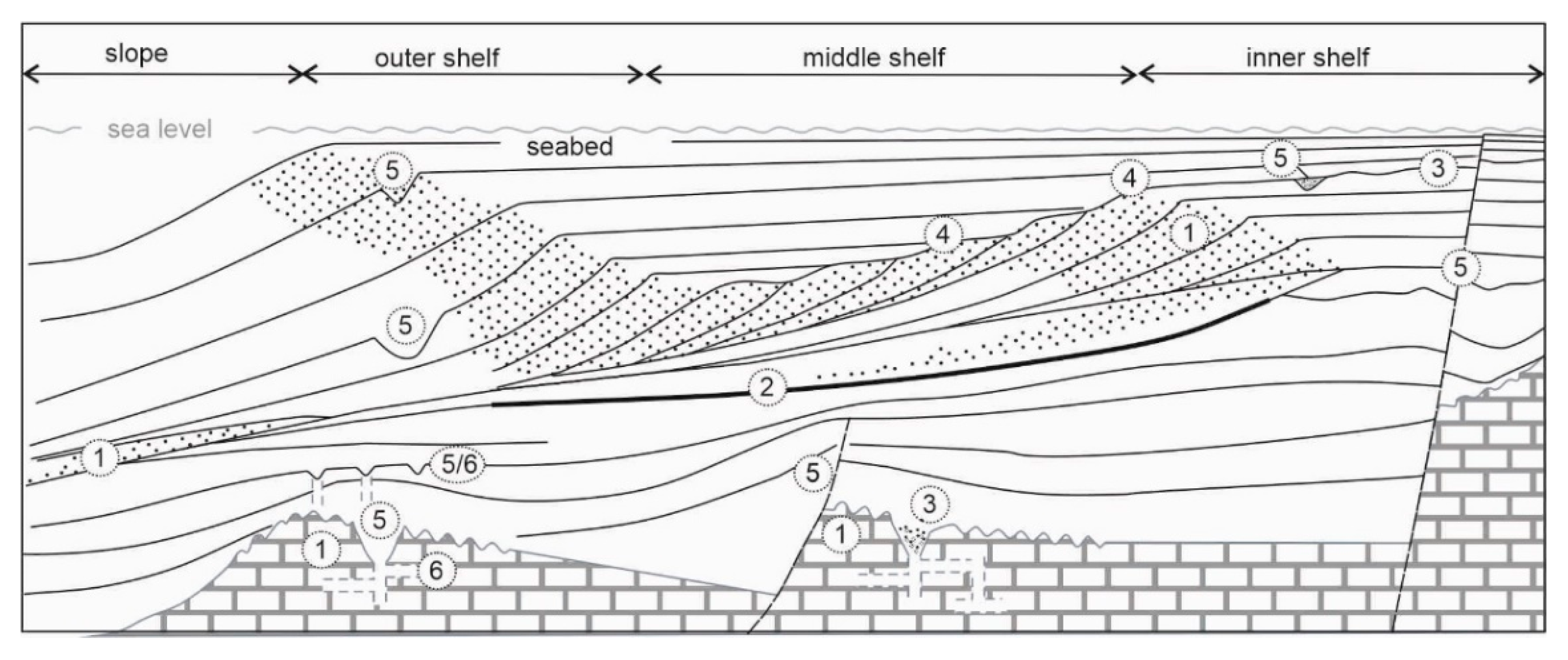
Figure 17.
Schematic cross geological section across part of a passive continental margin, showing the stratigraphic and morpho-structural elements detectable through seismic interpretation, which support the identification and mapping of low salinity aquifers. 1-Reservoir (aquifer), 2-Seal (aquitard/aquiclude), 3-Paleo-continental environments, 4-Paleo-coastline, 5-Conduits (e.g., canyons, valleys, channels, sinkholes, faults) 6-Aquifer indicators. See text for detailed explanation of each of these elements. Sequence stratigraphic framework modified from Reference [155].

The results of the considered case studies are currently biased towards aquifers hosted in siliciclastic sedimentary units, as these settings have been better surveyed and calibrated compared to offshore karstic aquifers, whose architecture remains much less predictable. In clastic continental margins settings, clinothems exert an important structural control on the lateral and vertical extent of low-salinity groundwater (e.g., New Jersey and Martha’s Vineyard case studies). Coarser grain-size sediments, with high porosity and permeability, are naturally suited for storage of buried fluids (e.g., Section 3.1.2). According to facies and sequence stratigraphic models, these sediments are most likely to be deposited during regressions and are often separated by maximum flooding surfaces. Clinoform topsets or other high porosity and permeability bodies (such as basin floor fans) are reservoirs for low salinity waters. This is the case in the Pliocene sands on the Mediterranean offshore Southern France and on the New Jersey inner shelf. However, due to their high permeability, they are also subject to density driven sea-water intrusion, as it is the case in the New Jersey middle shelf, that is, in a more distal area with limited connection to the onshore recharge.
In the case on the New Jersey inner shelf, the modern onshore hydraulic system is thought to extend offshore in both the coarse and fine grained fraction of the clinothems. Further offshore, the presence of salt water in the coarse grained fractions of the topsets has tentatively been explained by seawater penetration as a result of fast vertical density-driven flow [17]. In this case, the vertical flow would be expected to be greater than any horizontal, land-to-sea directed flow within the connected reservoirs. Diffusion is also sometimes accounted for the low salinity water hosted in mid-low permeability sediments including silts and clays. In summary, the emplacement and preservation of bodies of freshened groundwater is complex and depends on the timing of emplacement, 3D reservoir geometry, present-day connection to the sea and the presence of tight layers which may aid the preservation of freshwater aquifers.
As a general rule, the preservation of low-salinity pore waters is inversely proportional to the age/depth of sediments. Well defined stratigraphic boundaries such as unconformities, lateral and vertical facies changes and more specifically, maximum flooding and transgressive surfaces marking a shift to fine-grained facies or diagenetic boundaries, can seal the aquifer and constrain the upward extent of low-salinity aquifers. The role of low-permeability barriers (intra or extra-formational) to separate superimposed aquifers is shown in the Tanzania/Zanzibar and New Jersey case studies. This phenomenon has also been observed elsewhere, such as in Hong Kong [156,157,158].
Evaporites, which are considered a good seal for petroleum fluids, when in contact with undersaturated pore fluids, are prone to quick dissolution and produce salinization of offshore freshened groundwater [159,160]. This upwelling-driven salinization process is recorded for example, offshore New Jersey. Evaporites (in particular, halite) have a very specific seismic expression and can be clearly identified on seismic data.
In carbonate systems, poro-permeability prediction based on seismic and sequence stratigraphy is more complex and highly variable. However, seismic data can image the presence of karstic geomorphological features, of freshwater vents associated to karstic conduits and of subaerially exposed shelves which might have hosted a freshwater aquifer in the past.
Although we have highlighted the benefits of integrating seismic analysis into offshore freshened water research, the use of seismic data in such studies is constrained by a number of factors that might limit its application to this field of study. These factors include—(1) the high economic cost of seismic data acquisition and processing, (2) the constraints posed by environmental regulations that vary across country boundaries and (3) the technical challenges for data acquisition in specific areas such as in shallow waters, for example, the transition zone and proximal part of continental shelves (few to 10 s of meters of seabed depth).
4.2. Integration with Petroleum Geology Studies
The large seismic database used in oil exploration could potentially bridge the previously described ‘data gap’, due to its spatial coverage and vast geographic availability [161]. Seismic data interpretation in offshore petroleum studies is mostly focused on hydrocarbon-bearing basins, normally at a deeper burial depth compared to the described freshened groundwater systems. However, the case studies described in the Gippsland basin and in Tanzania [144,151,152] provide clear examples of the how the integration of petroleum exploration data with offshore hydrogeology analysis can lead to a better understanding of onshore-offshore groundwater systems. Similarly, in Suriname [162] industry data support the characterization of lithologies acting as a seal both for petroleum fluids and for freshwater diffusion.
More in general, industry seismic and drilling data can provide further information on offshore aquifers through data on fluid pressures, on presence of permeability barriers, on the ‘hydrodynamic’ or ‘hydrostatic’ nature of aquifers and on the presence of fossil low salinity waters [22,23,25,161,163,164,165]. An example of deep low salinity water in a karst oil reservoir is recorded in the offshore drilling of the Rospo Mare structure (Adriatic Sea, about 30 km off the coast of Italy) at about 1300 m below sea-level, where heavy oil is trapped in Cretaceous karstic limestones. Most of these karst cavities are filled with fresh or slightly brackish water [18,166,167], which is thought to be directly connected with the Maiella limestone-rich mountains, where the aquifer is recharged, some 70 km to the NW of Rospo-Mare. Interestingly, this example is located in an active tectonic setting and differs from the classic passive margin case studies (e.g., New Jersey). Therefore, the role played by relative sea-level changes, such as in back-arc or foreland basins, must be considered in relation to how the tectonic tilting or drowning might create favorable conditions for the recharge from landmasses [59,61,62].
Although there is a significant amount of seismic data already acquired on continental margins worldwide, a series of factors make the data still relatively inaccessible or of limited use to the scientific community studying offshore groundwater. These are primarily—(1) the limits imposed by confidentiality and proprietary nature of most of industry-derived data; (2) the differences in acquisition design, normally focused on deeper targets; and related to this, (3) the large heterogeneity of data quality and resolution.
4.3. Applicability and Future Avenues of Research
In this review we have described a number of case studies focused on the application of seismic methods in offshore freshened groundwater analysis. The same concepts can be applied to other areas of continental margins worldwide, where extensive literature and a wealth of case studies exist and have already defined the seismic and sequence stratigraphic setting and their structural contexts. However, the focus of these studies (e.g., reservoir characterization, paleoclimate, sea-level, paleoenvironments, structural evolution of continental margins) has not usually included offshore groundwater. Comprehensive, large-scale mapping of the sedimentary units hosting potential aquifers, based on these data, can be used to improve calculations of the volumes of fresh/brackish waters entrapped in continental margins, building on previous attempts [4,16,93,102].
Further avenues in offshore groundwater research can be created by extracting additional information from seismic data and by expanding the analysis to different areas of marine basins. Extracting additional information from seismic data can involve for example, a wider use of attribute analysis including quantitative methods. Quantitative seismic interpretation can be used to map permeability and porosity variation across a study area and provide an enhanced implementation of EM models, for example, through seismic inversion analysis. Porosity and permeability are key when modelling EM data to map offshore groundwater salinity and so far they can only be determined from borehole data, which have a very limited spatial extent. Increased accessibility of 3D seismic and well calibration would facilitate the use of these seismic attributes for offshore freshened groundwater mapping.
Proximal and shallow aquifers of freshened water, generally connected to onshore systems, are currently the most commonly observed sites for the occurrences of offshore low-salinity groundwater. A frontier area for freshened groundwater mapping is represented by deep offshore reservoirs, as the few case studies using hybrid industry/academic data have suggested. According to the literature, there are a series of factors that can lead to the presence of low-salinity water in deep and distal submarine sediments, far beyond the expected current limits. These factors include—(a) recharge during past sea-level lowstand [95], (b) entrapment of connate water in rapidly subsiding basins [139], (c) release of water by the dissociation of gas hydrates and other diagenetic reactions [79], glacier-related injection ([20] and references therein). Seismic data analysis can bring insights in these deeper aquifers, which could potentially host significant amount of freshened groundwater; however, they would be considered as paleo-groundwater resources and their exploitation regulated by economic, environmental, sustainability and recovery considerations.
Theoretically the methods reviewed here could be also applied to the analysis of freshened groundwater in shallower setting, such as the highly populated and urbanized land-sea “transition zone.” However, mapping this ‘white gap’ (between coast and shallow offshore area) can prove challenging because acquisition of seismic data is limited by technical and socio-economic factors. Overcoming these challenges will make seismic data in the land-sea transition zone increasingly available and provide new tools for understanding the global distribution of offshore freshened groundwater close to coastal communities.
Author Contributions
Conceptualization, C.B. and J.L., methodology, C.B., J.L., A.M. writing—original draft preparation, C.B. and J.L.; writing—review and editing, C.B., J.L., A.M., H.M. All authors have read and agreed to the published version of the manuscript.
Funding
C.B. was funded by Leverhulme trust, ‘Neptune’ project RPG-2018-24 and A.M. was funded by European Research Council (ERC) under the European Union’s Horizon 2020 research and innovation program (grant agreement No 677898 (MARCAN).
Acknowledgments
We would like to thank Geosciences Guest Editor Domenico Ridente, for inviting us to submit our contribution as an earlier version of this manuscript. Fridtjov Ruden, Angelo Camerlenghi and Mark Cuthbert are gratefully acknowledged for fruitful discussions and contributing to shape this project in its different phases.
Conflicts of Interest
The authors declare no conflict of interest.
References
- Pachauri, R.K.; Allen, M.R.; Barros, V.R.; Broome, J.; Cramer, W.; Christ, R.; Church, J.A.; Clarke, L.; Dahe, Q.; Dasgupta, P. Climate Change 2014: Synthesis Report. Contribution of Working Groups I, II and III to the Fifth Assessment Report of the Intergovernmental Panel on Climate Change; IPCC: Geneva, Switzerland, 2014. [Google Scholar]
- Polemio, M. Monitoring and management of karstic coastal groundwater in a changing environment (Southern Italy): A review of a regional experience. Water 2016, 8, 148. [Google Scholar] [CrossRef] [Green Version]
- Fisher, A.T. Marine hydrogeology: Recent accomplishments and future opportunities. Hydrogeol. J. 2005, 13, 69–97. [Google Scholar] [CrossRef]
- Post, V.E.; Groen, J.; Kooi, H.; Person, M.; Ge, S.; Edmunds, W.M. Offshore fresh groundwater reserves as a global phenomenon. Nature 2013, 504, 71–78. [Google Scholar] [CrossRef] [PubMed]
- Bear, J.; Cheng, A.H.-D.; Sorek, S.; Ouazar, D.; Herrera, I. Seawater Intrusion in Coastal Aquifers: Concepts, Methods and Practices; Springer Science & Business Media: Berlin, Germany, 1999; Volume 14. [Google Scholar]
- Barlow, P.M. Ground Water in Fresh Water-Salt Water Environments of the Atlantic; Geological Survey (USGS): Reston, VA, USA, 2003; Volume 1262.
- Ferguson, G.; Gleeson, T. Vulnerability of coastal aquifers to groundwater use and climate change. Nat. Clim. Chang. 2012, 2, 342–345. [Google Scholar] [CrossRef]
- Hinkelmann, R.; Sheta, H.; Class, H.; Helmig, R. A Comparison of Different Model Concepts for Saltwater Intrusion Processes; IAHS Publication: Wallingford, UK, 2000; pp. 385–391. [Google Scholar]
- Kouzana, L.; Benassi, R. Geophysical and hydrochemical study of the seawater intrusion in Mediterranean semi arid zones. Case of the Korba coastal aquifer (Cap-bon, Tunisia). J. Afr. Earth Sci. 2010, 58, 242–254. [Google Scholar] [CrossRef]
- Nowroozi, A.A.; Horrocks, S.B.; Henderson, P. Saltwater intrusion into the freshwater aquifer in the eastern shore of Virginia: A reconnaissance electrical resistivity survey. J. Appl. Geophys. 1999, 42, 1–22. [Google Scholar] [CrossRef]
- Vengosh, A.; Spivack, A.J.; Artzi, Y.; Ayalon, A. Geochemical and boron, strontium and oxygen isotopic constraints on the origin of the salinity in groundwater from the Mediterranean coast of Israel. Water Resour. Res. 1999, 35, 1877–1894. [Google Scholar] [CrossRef]
- Weinthal, E.; Vengosh, A.; Marei, A.; Gutierrez, A.; Kloppmann, W. The water crisis in the Gaza strip: Prospects for resolution. Groundwater 2005, 43, 653–660. [Google Scholar] [CrossRef]
- Werner, A.D.; Bakker, M.; Post, V.E.; Vandenbohede, A.; Lu, C.; Ataie-Ashtiani, B.; Simmons, C.T.; Barry, D.A. Seawater intrusion processes, investigation and management: Recent advances and future challenges. Adv. Water Resour. 2013, 51, 3–26. [Google Scholar] [CrossRef]
- Dugan, B.; Flemings, P.B. Overpressure and fluid flow in the New Jersey continental slope: Implications for slope failure and cold seeps. Science 2000, 289, 288–291. [Google Scholar] [CrossRef]
- Mountain, G.; Proust, J.; McInroy, D.; Cotterill, C. The Expedition 313 Scientists: Proceedings of Integrated Ocean Drilling Program, 313; Integrated Ocean Drilling Program Management International, Inc.: Tokyo, Japan, 2010. [Google Scholar]
- Cohen, D.; Person, M.; Wang, P.; Gable, C.W.; Hutchinson, D.; Marksamer, A.; Dugan, B.; Kooi, H.; Groen, K.; Lizarralde, D. Origin and extent of fresh paleowaters on the Atlantic continental shelf, USA. Groundwater 2010, 48, 143–158. [Google Scholar] [CrossRef] [PubMed]
- Lofi, J.; Inwood, J.; Proust, J.-N.; Monteverde, D.H.; Loggia, D.; Basile, C.; Otsuka, H.; Hayashi, T.; Stadler, S.; Mottl, M.J. Fresh-water and salt-water distribution in passive margin sediments: Insights from integrated ocean drilling program expedition 313 on the New Jersey margin. Geosphere 2013, 9, 1009–1024. [Google Scholar] [CrossRef] [Green Version]
- Vernet, R. Karst et hydrocarbures. Rospo mare: Un paleokarst pétrolier exploité en mer Adriatique (Italie). Geochronique 2000, 76, 34–35. [Google Scholar]
- Van Geldern, R.; Hayashi, T.; Böttcher, M.E.; Mottl, M.J.; Barth, J.A.; Stadler, S. Stable isotope geochemistry of pore waters and marine sediments from the New Jersey shelf: Methane formation and fluid origin. Geosphere 2013, 9, 96–112. [Google Scholar] [CrossRef]
- Bakken, T.H.; Ruden, F.; Mangset, L.E. Submarine groundwater: A new concept for the supply of drinking water. Water Resour. Manag. 2012, 26, 1015–1026. [Google Scholar] [CrossRef]
- Berndt, C.; Micallef, A. Could offshore groundwater rescue coastal cities? Nature 2019, 574, 36. [Google Scholar] [CrossRef] [Green Version]
- Tóth, J. Gravitational Systems of Groundwater Flow: Theory, Evaluation, Utilization; Cambridge University Press: Cambridge, UK, 2009. [Google Scholar]
- Harrison, W.J.; Summa, L.L. Paleohydrology of the Gulf of Mexico basin. Am. J. Sci. 1991, 291, 109–176. [Google Scholar] [CrossRef]
- Jowett, E.C.; Cathles III, L.M.; Davis, B.W. Predicting depths of gypsum dehydration in evaporitic sedimentary basins. Am. Assoc. Pet. Geol. Bull. 1993, 77, 402–413. [Google Scholar]
- Bjørlykke, K. Fluid flow in sedimentary basins. Sediment. Geol. 1993, 86, 137–158. [Google Scholar] [CrossRef]
- Colten-Bradley, V.A. Role of pressure in smectite dehydration—Effects on geopressure and smectite-to-illite transformation. AAPG Bull. 1987, 71, 1414–1427. [Google Scholar]
- Kastner, M.; Gieskes, J. Opal-a to opal-ct transformation: A kinetic study. In Developments in Sedimentology; Elsevier: Amsterdam, The Netherlands, 1983; Volume 36, pp. 211–227. [Google Scholar]
- Davies, R.J.; Cartwright, J. A fossilized opal a to opal c/t transformation on the northeast atlantic margin: Support for a significantly elevated palaeogeothermal gradient during the Neogene? Basin Res. 2002, 14, 467–486. [Google Scholar] [CrossRef]
- Micallef, A.; Mountjoy, J.; Schwalenberg, K.; Jegen, M.; Weymer, B.; Woelz, S.; Gerring, P.; Luebben, N.; Spatola, D.; Cunarro Otero, D. How Offshore Groundwater Shapes the Seafloor. Eos Earth Space Sci. News 2018, 99, 8. [Google Scholar] [CrossRef] [Green Version]
- Moore, W.S. The effect of submarine groundwater discharge on the ocean. Annu. Rev. Mar. Sci. 2010, 2, 59–88. [Google Scholar] [CrossRef] [PubMed] [Green Version]
- Micallef, A.; Person, M.; Haroon, A.; Weymer, B.; Jegen, M.; Schwalenberg, K.; Faghih, K.; Duan, S.; Cohen, D.; Mountjoy, J.; et al. 3d characterisation and quantification of an offshore freshened groundwater system in the Canterbury Bight. Nat. Commun. 2020, 11, 1372. [Google Scholar] [CrossRef] [PubMed] [Green Version]
- Harrar, W.; Williams, A.; Barker, J.; Van Camp, M. Modelling scenarios for the emplacement of palaeowaters in aquifer systems. Geol. Soc. Lond. Spec. Publ. 2001, 189, 213–229. [Google Scholar] [CrossRef]
- Ingebritsen, S.; Sanford, W.; Neuzil, C. Groundwater in Geological Processes; Cambridge Univ. Press: Cambridge, UK, 2006; p. 562. [Google Scholar]
- Bratton, J.F. The three scales of submarine groundwater flow and discharge across passive continental margins. J. Geol. 2010, 118, 565–575. [Google Scholar] [CrossRef] [Green Version]
- Destouni, G.; Prieto, C. On the possibility for generic modeling of submarine groundwater discharge. Biogeochemistry 2003, 66, 171–186. [Google Scholar] [CrossRef]
- Moore, W.S.; Shaw, T.J. Chemical signals from submarine fluid advection onto the continental shelf. J. Geophys. Res. Ocean. 1998, 103, 21543–21552. [Google Scholar] [CrossRef]
- Moosdorf, N.; Oehler, T. Societal use of fresh submarine groundwater discharge: An overlooked water resource. Earth Sci. Rev. 2017, 171, 338–348. [Google Scholar] [CrossRef]
- Taniguchi, M.; Burnett, W.C.; Cable, J.E.; Turner, J.V. Investigation of submarine groundwater discharge. Hydrol. Process. 2002, 16, 2115–2129. [Google Scholar] [CrossRef]
- Younger, P.L.; Moore, W.S.; Church, T.M. Submarine groundwater discharge. Nature 1996, 382, 121. [Google Scholar] [CrossRef]
- Edmunds, W. Palaeowaters in european coastal aquifers—The goals and main conclusions of the Palaeaux project. Geol. Soc. Lond. Spec. Publ. 2001, 189, 1–16. [Google Scholar] [CrossRef]
- Saffer, D. Hydrostratigraphy as a control on subduction zone mechanics through its effects on drainage: An example from the Nankai margin, sw Japan. Geofluids 2010, 10, 114–131. [Google Scholar]
- Edmunds, W.M.; Milne, C. Palaeowaters in Coastal Europe: Evolution of Groundwater Since the Late Pleistocene; Geological Society of London: London, UK, 2001. [Google Scholar]
- Brown, A.R. Interpretation of Three-Dimensional Seismic Data, 6th ed.; AAPG: Tulsa, OK, USA, 2004. [Google Scholar]
- Emery, D.; Myers, K. Sequence Stratigraphy; John Wiley & Sons: Hoboken, NJ, USA, 2009. [Google Scholar]
- Duncan, P.M. Part 7. Geophysical Methods. In Development Geology Reference Manual; AAPG: Tulsa, OK, USA, 1992; Volume ME 10, p. 357. [Google Scholar]
- Micallef, A. Marine geomorphology: Geomorphological mapping and the study of submarine landslides. In Developments in Earth Surface Processes; Elsevier: Amsterdam, The Netherlands, 2011; Volume 15, pp. 377–395. [Google Scholar]
- Posamentier, H.W.; Davies, R.J.; Cartwright, J.A.; Wood, L.J. Seismic Geomorphology—An Overview; Geological Society London Special Publications: London, UK, 2007; Volume 277, pp. 1–14. [Google Scholar]
- Catuneanu, O. Sequence Stratigraphy: Guidelines for a Standard Methodology. In Stratigraphy Timescales; Elsevier: Amsterdam, The Netherlands, 2017; Volume 2, pp. 1–57. [Google Scholar]
- Catuneanu, O.; Abreu, V.; Bhattacharya, J.; Blum, M.; Dalrymple, R.; Eriksson, P.; Fielding, C.R.; Fisher, W.; Galloway, W.; Gibling, M. Towards the Standardization of Sequence Stratigraphy. Earth Sci. Rev. 2009, 92, 1–33. [Google Scholar] [CrossRef] [Green Version]
- Helland-Hansen, W.; Martinsen, O.J. Shoreline trajectories and sequences: Description of variable depositional-dip scenarios. J. Sediment. Res. 1996, 66, 670–688. [Google Scholar]
- Embry, A.; Johannessen, E. T–r sequence stratigraphy, facies analysis and reservoir distribution in the uppermost Triassic–lower Jurassic succession, western Sverdrup basin, arctic Canada. In Norwegian Petroleum Society Special Publications; Elsevier: Amsterdam, The Netherlands, 1993; Volume 2, pp. 121–146. [Google Scholar]
- Hubbard, R.J.; Pape, J.; Roberts, D.G. Depositional Sequence Mapping as a Technique to Establish Tectonic and Stratigraphic Framework and Evaluate Hydrocarbon Potential on a Passive Continental Margin: Chapter 5; AAPG: Tulsa, OK, USA, 1985. [Google Scholar]
- Neal, J.; Abreu, V. Sequence stratigraphy hierarchy and the accommodation succession method. Geology 2009, 37, 779–782. [Google Scholar] [CrossRef]
- Salvador, A. A Guide to Stratigraphic Classification, Terminology and Procedure; IUGS: Boulder, CO, USA, 1994. [Google Scholar]
- Loucks, R.G.; Sarg, J.F. Carbonate Sequence Stratigraphy: Recent Developments and Applications, AAPG Memoir 57; AAPG: Tulsa, OK, USA, 1983. [Google Scholar]
- Pomar, L. High-resolution sequence stratigraphy in prograding Miocene carbonates: Application to seismic interpretation. Carbonate Seq. Stratigr. Recent Dev. Appl. AAPG Mem. 1993, 57, 389–407. [Google Scholar]
- Sarg, J. Carbonate Sequence Stratigraphy; AAPG: Tulsa, OK, USA, 1988. [Google Scholar]
- Schumm, S. River response to baselevel change: Implications for sequence stratigraphy. J. Geol. 1993, 101, 279–294. [Google Scholar] [CrossRef]
- Catuneanu, O.; Sweet, A.R.; Miall, A.D. Concept and styles of reciprocal stratigraphies: Western Canada foreland system. Terra Nova Oxford 1999, 11, 1–8. [Google Scholar] [CrossRef]
- Madof, A.S.; Christie-Blick, N.; Anders, M.H. Tectonically controlled nearshore deposition: Cozzette sandstone, Book Cliffs, Colorado, USA. J. Sediment. Res. 2015, 85, 459–488. [Google Scholar] [CrossRef] [Green Version]
- Rossi, M.; Minervini, M.; Ghielmi, M. Drowning unconformities on hinged clastic shelves. Geology 2018, 46, 439–442. [Google Scholar] [CrossRef]
- Madof, A.S.; Harris, A.D.; Connell, S.D. Nearshore along-strike variability: Is the concept of the systems tract unhinged? Geology 2016, 44, 315–318. [Google Scholar] [CrossRef] [Green Version]
- Catuneanu, O. Principles of Sequence Stratigraphy; Elsevier: Amsterdam, The Netherlands, 2006. [Google Scholar]
- Schlager, W. Type 3 sequence boundaries. Spec. Publ. Soc. Econ. Paleontol. Mineral. 1999, 63, 35–46. [Google Scholar]
- Vail, P. The stratigraphic signatures of tectonics, eustacy and sedimentology—An overview. In Cycles and Events in Stratigraphy; Einsele, G., Ricken, W., Seilacher, A., Eds.; Springer: Berlin, Germay; London, UK, 1991; pp. 617–659. [Google Scholar]
- Ridente, D.; Trincardi, F. Eustatic and tectonic control on deposition and lateral variability of Quaternary regressive sequences in the Adriatic basin (Italy). Mar. Geol. 2002, 184, 273–293. [Google Scholar] [CrossRef]
- Haq, B.U.; Hardenbol, J.; Vail, P.R. Chronology of fluctuating sea levels since the Triassic. Science 1987, 235, 1156–1167. [Google Scholar] [CrossRef] [Green Version]
- Mavko, G.; Mukerji, T.; Dvorkin, J. The Rock Physics Handbook: Tools for Seismic Analysis in Porous Media; Cambridge University Press: Cambridge, MA, USA, 2003. [Google Scholar]
- Avseth, P.; Mukerji, T.; Mavko, G. Quantitative Seismic Interpretation: Applying Rock Physics Tools to Reduce Interpretation Risk; Cambridge University Press: Cambridge, UK, 2010. [Google Scholar]
- Thomas, A.; Reiche, S.; Riedel, M.; Clauser, C. The fate of submarine fresh groundwater reservoirs at the New Jersey shelf, USA. Hydrogeol. J. 2019, 27, 2673–2694. [Google Scholar] [CrossRef]
- Miller, K.G.; Browning, J.V.; Mountain, G.S.; Bassetti, M.A.; Monteverde, D.; Katz, M.E.; Inwood, J.; Lofi, J.; Proust, J.-N. Sequence boundaries are impedance contrasts: Core-seismic-log integration of Oligocene–Miocene sequences, New Jersey shallow shelf. Geosphere 2013, 9, 1257–1285. [Google Scholar] [CrossRef]
- Evans, R.L.; Lizarralde, D. Geophysical evidence for karst formation associated with offshore groundwater transport: An example from North Carolina. Geochem. Geophys. Geosyst. 2003, 4. [Google Scholar] [CrossRef]
- Lofi, J.; Pezard, P.; Bouchette, F.; Raynal, O.; Sabatier, P.; Denchik, N.; Levannier, A.; Dezileau, L.; Certain, R. Integrated onshore-offshore investigation of a Mediterranean layered coastal aquifer. Groundwater 2013, 51, 550–561. [Google Scholar] [CrossRef]
- Mulligan, A.E.; Evans, R.L.; Lizarralde, D. The role of paleochannels in groundwater/seawater exchange. J. Hydrol. 2007, 335, 313–329. [Google Scholar] [CrossRef]
- Land, L.; Paull, C. Submarine karst belt rimming the continental slope in the Straits of Florida. Geo-Mar. Lett. 2000, 20, 123–132. [Google Scholar] [CrossRef]
- Lofi, J.; Berné, S.; Tesson, M.; Seranne, M.; Pezard, P. Giant solution-subsidence structure in the western Mediterranean related to deep substratum dissolution. Terra Nova 2012, 24, 181–188. [Google Scholar] [CrossRef]
- Swarzenski, P.; Reich, C.; Spechler, R.; Kindinger, J.; Moore, W. Using multiple geochemical tracers to characterize the hydrogeology of the submarine spring off Crescent Beach, Florida. Chem. Geol. 2001, 179, 187–202. [Google Scholar] [CrossRef]
- Hovland, M.; Judd, A.G. Seabed Pockmarks and Seepages: Impact on Geology, Biology and the Marine Environment; Graham & Trotman: London, UK, 1988. [Google Scholar]
- Judd, A.G.; Hovland, M. Seabed Fluid Flow: The Impact on Geology, Biology and the Marine Environment; Cambridge University Press: Cambridge, MA, USA, 2007; p. 1. [Google Scholar]
- Micallef, A.; Foglini, F.; Le Bas, T.; Angeletti, L.; Maselli, V.; Pasuto, A.; Taviani, M. The submerged paleolandscape of the maltese islands: Morphology, evolution and relation to Quaternary environmental change. Mar. Geol. 2013, 335, 129–147. [Google Scholar] [CrossRef]
- Land, L.A.; Paull, C.K.; Hobson, B. Genesis of a submarine sinkhole without subaerial exposure: Straits of Florida. Geology 1995, 23, 949–951. [Google Scholar] [CrossRef]
- Plummer, L. Mixing of sea water with calcium carbonate ground water. Geol. Soc. Am. Mem. 1975, 142, 219–236. [Google Scholar]
- Runnells, D.D. Diagenesis, chemical sediments and the mixing of natural waters. J. Sediment. Res. 1969, 39, 1188–1201. [Google Scholar]
- Micallef, A.; Georgiopoulou, A.; Bas, T.P.L.; Mountjoy, J.J.; Huvenne, V.A.; Iacono, C.L. Processes on the Precipice: Seafloor Dynamics Across the Upper Malta-Sicily Escarpment. In Proceedings of the CIESM 2013, Marseille, France, 28 October–1 November 2013. [Google Scholar]
- Audra, P.; Mocochain, L.; Camus, H.; Gilli, É.; Clauzon, G.; Bigot, J.-Y. The effect of the Messinian deep stage on karst development around the Mediterranean sea. Examples from southern France. Geodin. Acta 2004, 17, 389–400. [Google Scholar] [CrossRef] [Green Version]
- Cavalera, T.; Gilli, E.; Mamindy-Pajany, Y.; Marmier, N. Mechanism of salt contamination of karstic springs related to the messinian deep stage. The speleological model of Port Miou (France). Geodin. Acta 2010, 23, 15–28. [Google Scholar] [CrossRef]
- Gilli, É.; Audra, P. Les lithophages Pliocènes de la Fontaine de Vaucluse (Vaucluse, France). Un argument pour une phase Messinienne dans la genèse du plus grand karst noyé de France. C. R. Geosci. 2004, 336, 1481–1489. [Google Scholar] [CrossRef]
- Mocochain, L.; Audra, P.; Bigot, J.-Y. Base level rise and per ascensum model of speleogenesis (pams). Interpretation of deep phreatic karsts, vauclusian springs and chimney-shafts. Bull. Société Géologique Fr. 2011, 182, 87–93. [Google Scholar] [CrossRef] [Green Version]
- Hovland, M. Geomorphological, geophysical and geochemical evidence of fluid flow through the seabed. J. Geochem. Explor. 2003, 78, 287–291. [Google Scholar] [CrossRef]
- Schumacher, D. Hydrocarbon-Induced Alteration of Soils and Sediments; AAPG: Tulsa, OK, USA, 1996. [Google Scholar]
- Reusch, A.; Loher, M.; Bouffard, D.; Moernaut, J.; Hellmich, F.; Anselmetti, F.S.; Bernasconi, S.M.; Hilbe, M.; Kopf, A.; Lilley, M.D. Giant lacustrine pockmarks with subaqueous groundwater discharge and subsurface sediment mobilization. Geophys. Res. Lett. 2015, 42, 3465–3473. [Google Scholar] [CrossRef] [Green Version]
- Hathaway, J.C.; Poag, C.W.; Valent, P.C.; Miller, R.E.; Schultz, D.M.; Manhe, F.T.; Kohout, F.A.; Bothner, M.H.; Sangi, D.A. US Geological Survey core drilling on the Atlantic shelf. Science 1979, 206, 2. [Google Scholar] [CrossRef]
- Kohout, F.; Hathaway, J.; Folger, D.; Bothner, M.; Walker, E.; Delaney, D.; Frimpter, M.; Weed, E.; Rhodehamel, E. Fresh ground water stored in aquifers under the continental shelf: Implications from a deep test, Nantucket island, Massachusetts. J. Am. Water Resour. Assoc. 1977, 13, 373–386. [Google Scholar] [CrossRef]
- Perlmutter, N.M.; Geraghty, J.J. Geology and Ground-Water Conditions in Southern Nassau and Southeastern Queens Counties, Long Island, New York; USGPO: Washington, DC, USA, 1963.
- Person, M.; Dugan, B.; Swenson, J.B.; Urbano, L.; Stott, C.; Taylor, J.; Willett, M. Pleistocene hydrogeology of the Atlantic continental shelf, New England. Geol. Soc. Am. Bull. 2003, 115, 1324–1343. [Google Scholar] [CrossRef]
- Person, M.; Taylor, J.Z.; Dingman, S.L. Sharp interface models of salt water intrusion and wellhead delineation on Nantucket Island, Massachusetts. Groundwater 1998, 36, 731–742. [Google Scholar] [CrossRef]
- Smolensky, D.A.; Buxton, H.T.; Shernoff, P.K. Hydrologic Framework of Long Island, New York; USGS: Reston, VA, USA, 1990. [CrossRef]
- Miller, K.G.; Kominz, M.A.; Browning, J.V.; Wright, J.D.; Mountain, G.S.; Katz, M.E.; Sugarman, P.J.; Cramer, B.S.; Christie-Blick, N.; Pekar, S.F. The Phanerozoic Record of Global Sea-Level Change. Science 2005, 310, 1293–1298. [Google Scholar] [CrossRef] [Green Version]
- Miller, K.G.; Mountain, G.S.; Wright, J.D.; Browning, J.V. A 180-million-year record of sea level and ice volume variations from continental margin and Deep-Sea isotopic records. Oceanography 2011, 24, 40–53. [Google Scholar] [CrossRef]
- Manheim, F.; Hall, R. Deep Evaporitic Strata off New York and New Jersey—Evidence from Interstitial Water Chemistry of Drill Cores. J. Res. 1976, 4, 697–702. [Google Scholar]
- Barton, G.J.; Storck, D.A.; Paulachok, G.N. Records of Wells, Exploratory Boreholes and Ground-Water Quality, Atlantic County and Vicinity, New Jersey; 2331-1258; US Geological Survey; Books and Open-File Reports Section [distributor]: Reston, VA, USA, 1993. [Google Scholar]
- Szabo, Z.; Keller, E.A.; Defawe, R.M. Pore-Water Quality in the Clay-Silt Confining Units of the Lower Miocene Kirkwood Formation and Hypothetical Effects on Water Quality in the Atlantic City 800-Foot Sand, Northeastern Cape May County, New Jersey; USGS: Reston, VA, USA, 2001. [CrossRef]
- Sugarman, P.J.; Miller, K.G.; Browning, J.V.; Kulpecz, A.A.; McLaughlin, P.P.; Monteverde, D.H. Hydrostratigraphy of the New Jersey coastal plain: Sequences and facies predict continuity of aquifers and confining units. Stratigraphy 2005, 2, 259–275. [Google Scholar]
- Gustafson, C.; Key, K.; Evans, R.L. Aquifer systems extending far offshore on the US Atlantic Margin. Sci. Rep. 2019, 9, 8709. [Google Scholar] [CrossRef] [PubMed]
- Kooi, H.; Groen, J. Offshore continuation of coastal groundwater systems; predictions using sharp-interface approximations and variable-density flow modelling. J. Hydrol. 2001, 246, 19–35. [Google Scholar] [CrossRef]
- Riedel, M.; Reiche, S.; Aßhoff, K.; Buske, S. Seismic depth imaging of sequence boundaries beneath the New Jersey shelf. Mar. Geophys. Res. 2019, 40, 17–32. [Google Scholar] [CrossRef]
- Pierre, C.; Blanc-Valleron, M.-M.; Boudouma, O.; Lofi, J. Carbonate and silicate cementation of siliciclastic sediments of the New Jersey shelf (IODP expedition 313): Relation with organic matter diagenesis and submarine groundwater discharge. Geo-Mar. Lett. 2017, 37, 537–547. [Google Scholar] [CrossRef]
- Guswa, J.H.; LeBlanc, D.R. Digital Models of Ground-Water Flow in the Cape Cod Aquifer System, Massachusetts; US Government Printing Office: Washington, DC, USA, 1985.
- Hall, R.E.; Poppe, L.J.; Ferrebee, W.M. A Stratigraphic Test Well, Martha’s Vineyard, Massachusetts: Description of Pleistocene to Upper Cretaceous Sediments Recovered from 262 Meters of Test Coring; US Government Printing Office: Washington, DC, USA, 1979.
- Mulligan, A.; Uchupi, E. New interpretation of glacial history of Cape Cod may have important implications for groundwater contaminant transport. Eos Trans. Am. Geophys. Union 2003, 84, 177–183. [Google Scholar] [CrossRef]
- Person, M.; Marksamer, A.; Dugan, B.; Sauer, P.E.; Brown, K.; Bish, D.; Licht, K.J.; Willett, M. Use of a vertical δ 18 o profile to constrain hydraulic properties and recharge rates across a glacio-lacustrine unit, Nantucket Island, Massachusetts, USA. Hydrogeol. J. 2012, 20, 325–336. [Google Scholar] [CrossRef]
- Person, M.; McIntosh, J.; Bense, V.; Remenda, V. Pleistocene hydrology of North America: The role of ice sheets in reorganizing groundwater flow systems. Rev. Geophys. 2007, 45. [Google Scholar] [CrossRef] [Green Version]
- Folger, D.W.; Hathaway, J.; Christopher, R.; Valentine, P.; Poag, C. Stratigraphic Test Well, Nantucket Island, Massachusetts; US Geological Survey: Reston, VA, USA, 1978; pp. 2330–5703.
- Denton, G.H.; Hughes, T.J. The Last Great Ice Sheets; Wiley: Hoboken, NJ, USA, 1981. [Google Scholar]
- Christie-Blick, N.; Austin, J.A., Jr.; Party, S.S. Introduction: Oligocene to Pleistocene Eustatic Change at the New Jersey Continental Margin—A Test of Sequence Stratigraphy; Columbia University: New York, NY, USA, 1998. [Google Scholar]
- Schlee, J.; Fritsch, J. Seismic Stratigraphy of the Georges Bank Basin Complex, Offshore New England: Rifted Margins: Field Investigations of Margin Structure and Stratigraphy; AAPG: Tulsa, OK, USA, 1982. [Google Scholar]
- Siegel, J.; Person, M.; Dugan, B.; Cohen, D.; Lizarralde, D.; Gable, C. Influence of late Pleistocene glaciations on the hydrogeology of the continental shelf offshore Massachusetts, USA. Geochem. Geophys. Geosystems 2014, 15, 4651–4670. [Google Scholar] [CrossRef] [Green Version]
- Siegel, J.; Dugan, B.; Lizarralde, D.; Person, M.; DeFoor, W.; Miller, N. Geophysical evidence of a late Pleistocene glaciation and paleo-ice stream on the Atlantic continental shelf offshore Massachusetts, USA. Mar. Geol. 2012, 303, 63–74. [Google Scholar] [CrossRef]
- Metzger, J.; Flemings, P.B.; Christie-Blick, N.; Mountain, G.S.; Austin, J., Jr.; Hesselbo, S. Late Miocene to pleistocene sequences at the New Jersey outer continental shelf (ODP leg 174a, sites 1071 and 1072). Sediment. Geol. 2000, 134, 149–180. [Google Scholar] [CrossRef] [Green Version]
- Marksamer, A. Integrating Geophysical, Hydrochemical and Hydrologic Data to Understand the Freshwater Resources on Nantucket Island, Massachusetts; Indiana University: Bloomington, IN, USA, 2007. [Google Scholar]
- Cable, J.E.; Burnett, W.C.; Chanton, J.P.; Weatherly, G.L. Estimating groundwater discharge into the northeastern Gulf of Mexico using radon-222. Earth Planet. Sci. Lett. 1996, 144, 591–604. [Google Scholar] [CrossRef]
- Johnston, R.H. The saltwater-freshwater interface in the tertiary limestone aquifer, southeast Atlantic outer-continental shelf of the USA. J. Hydrol. 1983, 61, 239–249. [Google Scholar] [CrossRef]
- Leve, G.W. Relation of concealed faults to water quality and the formation of solution features in the Floridan aquifer, northeastern Florida, USA. J. Hydrol. 1983, 61, 251–264. [Google Scholar] [CrossRef]
- Stringfield, V.T. Artesian Water in Tertiary Limestone in the Southeastern States; US Government Printing Office: Washington, DC, USA, 1966.
- Meisburger, E.P.; Field, M.E. Neogene sediments of atlantic inner continental shelf off northern Florida. AAPG Bull. 1976, 60, 2019–2037. [Google Scholar]
- Manheim, F.T.; Krantz, D.E.; Bratton, J.F. Studying ground water under Delmarva Coastal Bays using electrical resistivity. Groundwater 2004, 42, 1052–1068. [Google Scholar] [CrossRef]
- Rosenau, J.C.; Faulkner, G.L.; Hendry, C.W., Jr.; Hull, R.W. Springs of Florida; Florida Department of Natural Resources: Bureau of Geology: Tallahassee, FL, USA, 1977; Volume xxvii, p. 461. [Google Scholar]
- Meisler, H.; Leahy, P.P.; Knobel, L.L. Effect of Eustatic Sea-Level Changes on Saltwater-Freshwater Relations in the Northern Atlantic Coastal Plain; US Government Printing Office: Washington, DC, USA, 1984; Volume 2255.
- Land, L. Processes and Manifestations of Fluid Exchange within Passive Continental Margins; University of North Carolina: Chapel Hill, NC, USA, 2000. [Google Scholar]
- Bakalowicz, M. Karst at depth below the sea level around the Mediterranean due to the Messinian crisis of salinity. Hydrogeological consequences and issues. Geol. Belg. 2014, 17, 1374–8505. [Google Scholar]
- Garing, C.; Luquot, L.; Pezard, P.; Gouze, P. Geochemical investigations of saltwater intrusion into the coastal carbonate aquifer of Mallorca, Spain. Appl. Geochem. 2013, 39, 1–10. [Google Scholar] [CrossRef]
- Aunay, B.; Dörfliger, N.; Duvail, C.; Grelot, F.; Le Strat, P.; Montginoul, M.; Rinaudo, J.-D. A multidisciplinary approach for assessing the risk of seawater intrusion in coastal aquifers: The case of the Roussillon basin (France). Aquifer Syst. Manag. Darcy’s Leg. World Impending Water Short. Sel. Papers Hydrogeol. 2007, 10, 459. [Google Scholar]
- Duvail, C.; Gorini, C.; Lofi, J.; Le Strat, P.; Clauzon, G.; dos Reis, A.T. Correlation between onshore and offshore Pliocene–Quaternary systems tracts below the Roussillon basin (eastern Pyrenees, France). Mar. Pet. Geol. 2005, 22, 747–756. [Google Scholar] [CrossRef]
- El Yaouti, F.; El Mandour, A.; Khattach, D.; Benavente, J.; Kaufmann, O. Salinization processes in the unconfined aquifer of Bou-areg (ne Morocco): A geostatistical, geochemical and tomographic study. Appl. Geochem. 2009, 24, 16–31. [Google Scholar] [CrossRef]
- Petelet-Giraud, E.; Négrel, P.; Aunay, B.; Ladouche, B.; Bailly-Comte, V.; Guerrot, C.; Flehoc, C.; Pezard, P.; Lofi, J.; Dörfliger, N. Coastal groundwater salinization: Focus on the vertical variability in a multi-layered aquifer through a multi-isotope fingerprinting (roussillon basin, France). Sci. Total Environ. 2016, 566, 398–415. [Google Scholar] [CrossRef] [PubMed]
- Custodio, E. Coastal aquifers of europe: An overview. Hydrogeol. J. 2010, 18, 269–280. [Google Scholar] [CrossRef]
- Gladstone, R.; Flecker, R.; Valdes, P.; Lunt, D.; Markwick, P. The Mediterranean hydrologic budget from a late miocene global climate simulation. Palaeogeogr. Palaeoclimatol. Palaeoecol. 2007, 251, 254–267. [Google Scholar] [CrossRef]
- De Montety, V.; Radakovitch, O.; Vallet-Coulomb, C.; Blavoux, B.; Hermitte, D.; Valles, V. Origin of groundwater salinity and hydrogeochemical processes in a confined coastal aquifer: Case of the Rhône delta (southern France). Appl. Geochem. 2008, 23, 2337–2349. [Google Scholar] [CrossRef]
- Ruden, F. The discovery of a Neogene coastal aquifer in coastal Tanzania. Inst. Geol. Min. Esp. Coast. Aquifers Chall. Solut. 2007, 1, 363–372. [Google Scholar]
- Moe, H.; Ruden, F.; Gamache, M. Exploration and hydrogeological assessment of a deep coastal aquifer system in Tanzania. In Proceedings of the Congress of the International Association of Hydrogeologists, Dubrovnik, Croatia, 28 September 2017. [Google Scholar]
- Ruden, F. Freshwater entrapment in offshore Zanzibar basins. In International Symposium on Efficient Groundwater Resources Management; IGS-TH: Cambridge, UK, 2009. [Google Scholar]
- Woodroffe, S.A.; Horton, B.P. Holocene sea-level changes in the Indo-Pacific. J. Asian Earth Sci. 2005, 25, 29–43. [Google Scholar] [CrossRef] [Green Version]
- Voris, H.K. Maps of Pleistocene sea levels in southeast Asia: Shorelines, river systems and time durations. J. Biogeogr. 2000, 27, 1153–1167. [Google Scholar] [CrossRef] [Green Version]
- Moe, H.; Ruden, F. Use of exploration data for the assessment of deep groundwater resources in coastal Tanzania. In Irish Groundwater Newsletter; Geological Survey Ireland: Dublin, Ireland, 2009; pp. 3–10. [Google Scholar]
- Browne, G.H.; Naish, T.R. Facies development and sequence architecture of a late Quaternary fluvial-marine transition, Canterbury plains and shelf, New Zealand: Implications for forced regressive deposits. Sediment. Geol. 2003, 158, 57–86. [Google Scholar] [CrossRef]
- Lu, H.; Fulthorpe, C.S. Controls on sequence stratigraphy of a middle Miocene–Holocene, current-swept, passive margin: Offshore Canterbury basin, New Zealand. Geol. Soc. Am. Bull. 2004, 116, 1345–1366. [Google Scholar] [CrossRef]
- McHugh, C.M.; Fulthorpe, C.S.; Hoyanagi, K.; Blum, P.; Mountain, G.S.; Miller, K.G. The sedimentary imprint of Pleistocene glacio-eustasy: Implications for global correlations of seismic sequences. Geosphere 2018, 14, 265–285. [Google Scholar] [CrossRef]
- Villaseñor, T.; Jaeger, J.M.; Marsaglia, K.M.; Browne, G.H. Evaluation of the relative roles of global versus local sedimentary controls on middle to late Pleistocene formation of continental margin strata, Canterbury basin, New Zealand. Sedimentology 2015, 62, 1118–1148. [Google Scholar] [CrossRef]
- Barnes, A. Seismic Attributes in Your Facies: Canadian Society of Exploration Geophysicists Recorder 26. 2001. Available online: https://csegrecorder.com/articles/view/seismic-attributes-in-your-facies (accessed on 8 April 2020).
- Fulthorpe, C.; Hoyanagi, K.; Blum, P. Expedition IO. IODP expedition 317: Exploring the record of sea-level change off New Zealand. Sci. Drill. 2011, 12, 4–14. [Google Scholar] [CrossRef]
- Varma, S.; Michael, K. Impact of multi-purpose aquifer utilisation on a variable-density groundwater flow system in the Gippsland basin, Australia. Hydrogeol. J. 2012, 20, 119–134. [Google Scholar] [CrossRef]
- Nahm, G.Y. The Hydrogeology of the Gippsland Basin and Its Role in the Genesis and Accumulation of Petroleum. Ph.D. Thesis, School of Earth Sciences, The University of Melbourne, Parkville, Australia, 2002. Available online: http://hdl.handle.net/11343/39277 (accessed on 8 April 2020).
- Gibson-Poole, C.; Svendsen, L.; Underschultz, J.; Watson, M.; Ennis-King, J.; Van Ruth, P.; Nelson, E.; Daniel, R.; Cinar, Y. Site characterisation of a basin-scale CO2 geological storage system: Gippsland basin, southeast Australia. Environ. Geol. 2008, 54, 1583–1606. [Google Scholar] [CrossRef]
- Divko, L.G.; O’Brien, G.; Harrison, M.; Hamilton, J. Evaluation of the regional top seal in the Gippsland basin: Implications for geological carbon storage and hydrocarbon prospectivity. APPEA J. 2010, 50, 463–486. [Google Scholar] [CrossRef]
- Zecchin, M.; Catuneanu, O. High-resolution sequence stratigraphy of clastic shelves i: Units and bounding surfaces. Mar. Pet. Geol. 2013, 39, 1–25. [Google Scholar] [CrossRef]
- Jiao, J.J.; Shi, L.; Kuang, X.; Lee, C.M.; Yim, W.W.-S.; Yang, S. Reconstructed chloride concentration profiles below the seabed in Hong Kong (China) and their implications for offshore groundwater resources. Hydrogeol. J. 2015, 23, 277–286. [Google Scholar] [CrossRef]
- Kwong, H.T.; Jiao, J.J.; Chan, L.S. A preliminary study on the offshore stratigraphy in Hong Kong and its hydrogeological implications. Environ. Earth Sci. 2016, 75, 975. [Google Scholar] [CrossRef]
- Kwong, H.T.; Jiao, J.J. Hydrochemical reactions and origin of offshore relatively fresh pore water from core samples in Hong Kong. J. Hydrol. 2016, 537, 283–296. [Google Scholar] [CrossRef]
- Warren, J.K. Evaporites: Sediments, Resources and Hydrocarbons: Sediments, Resources and Hydrocarbons; Springer: Berlin, Germany, 2006. [Google Scholar]
- Warren, J.K. Salt usually seals but sometimes leaks: Implications for mine and cavern stability in the short and long term. Earth Sci. Rev. 2016, 165, 302–341. [Google Scholar] [CrossRef]
- Bjørlykke, K.; Gran, K. Salinity variations in North Sea formation waters: Implications for large-scale fluid movements. Mar. Pet. Geol. 1994, 11, 5–9. [Google Scholar] [CrossRef]
- Groen, J.; Velstra, J.; Meesters, A. Salinization processes in paleowaters in coastal sediments of Suriname: Evidence from δ37cl analysis and diffusion modelling. J. Hydrol. 2000, 234, 1–20. [Google Scholar] [CrossRef]
- Bethke, C.M. Inverse hydrologic analysis of the distribution and origin of Gulf Coast-type geopressured zones. J. Geophys. Res. Solid Earth 1986, 91, 6535–6545. [Google Scholar] [CrossRef]
- Dahlberg, E.C. Applied Hydrodynamics in Petroleum Exploration; Springer Science & Business Media: Berlin, Germany, 2012. [Google Scholar]
- Evans, D. The Millennium Atlas: Petroleum Geology of the Central and Northern North Sea; A Project of the Geological Society of London, the Geological Survey of Denmark and Greenland and the Norwegian Petroleum Society; Geological Society: London, UK, 2003. [Google Scholar]
- Dubois, P.; Sorriaux, P.; Soudet, H.-J. Rospo mare (Adriatique): Un paléokarst pétrolier du domaine méditerranéen. Karstologia 1993, 21, 31–42. [Google Scholar] [CrossRef]
- Fournillon, A.; Bellentani, G.; Moccia, A.; Jumeaucourt, C.; Terdich, P.; Siliprandi, F.; Peruzzo, F. Characterization of a paleokarstic oil field (Rospo Mare, Italy): Sedimentologic and diagenetic outcomes and their integration in reservoir simulation. In Eurokarst 2016, Neuchâtel; Springer: Berlin, Germany, 2017; pp. 47–55. [Google Scholar]
Figure 1.
World map showing the distribution of vast meteoric offshore groundwater reserves (modified from Reference [4]), with case studies shown in this paper. In red: reserves proven by observational data, in green: reserves with brackish component highlighted by pore water analysis, in blue: significant meteoric offshore groundwater with indirect evidence based on onshore paleo-groundwater [4]. In black dashed circles: case studies that use offshore geophysical data for groundwater analysis and are described in this paper. The yellow transparent overlay shows the highest density coverage of seismic reflection data, mostly from industry-funded and confidentiality protected sources. This map only provides an approximation of data distribution and it represents a sub-set of data globally acquired (source: https://www.globalseismiclibrary.com/, https://pwdatalibraries.maps.arcgis.com/).

Figure 2.
Example of use of seismic stratigraphic and attribute analysis for lithology/facies prediction in groundwater research (modified after Reference [70]). (A) Amplitude of a seismic line across the New Jersey continental shelf (see case study in Section 3.1.1 of this paper). (B) Cosine of phase attribute with major systems tracts boundaries (including sequence boundaries and transgressive surfaces/maximum regression surfaces) labelled to highlight the correlation of key seismic sequence stratigraphic relationships. (C) Original systems tracts interpretation by Reference [70] overlain on seismic data. (D) Stochastically generated facies distribution. FSST falling stage systems tract, TST transgressive systems tract, HST highstand systems tract, LST lowstand systems tract. Horizons m1 to m4.1 correspond to interpreted sequence boundaries used to constrain the shelf model (nomenclature after [71]).

Figure 3.
Example of combination of high resolution seismic data (CHIRP seismic profiles, upper panels) and electromagnetic data (as apparent porosities, lower panels) illustrating the offshore extent of a paleochannel with no seabed expression and its relationship with groundwater (modified from Reference [74]). The data are from offshore North Carolina. In (A) (2.8 km offshore) the channel geometry is visualized through seismic data as concave upwards high amplitude reflections between the seabed and 0.025 s TWT. The related EM response of the channel shows an increase in porosity reflecting coarser grained material within the channel, particularly at the channel floor. (B) Transect located 1 km offshore, where the channel is located between the seabed and 0.015 s TWT, with an EM response more complex than (A), with an initial drop in porosity at the channel flanks, followed by an increase in mid-channel. The 40-m receiver shows a smooth decrease in porosity starting about 100 m either side of the channel. In the seismic sections, 6ms corresponds approximately to 5 m; resolution of data, considering frequency of 1–7 kHz and a typical shallow siliciclastic sediment velocity of 1600–1800 m/s, is in the order of few 10 s of cm.

Figure 4.
Examples of buried collapse structures. (A) High-resolution seismic profile of Crescent Beach Spring (Florida) and surrounding area. Resolution is not indicated in the cited work but it is likely to be in the order of 1 m considering a 500–2000 Hz source. The spring discharge is visible in the seismic image and the associated collapse feature (modified from Reference [77]). The horizontal scale is missing in the original figure, however, as a reference, the active spring vent related depression is ca. 150 m wide at the sea floor. (B) In the Gulf of Lions, buried collapse feature on a CHIRP profile (vertical resolution 2 to 5.2 kHz, i.e., 30–50 cm), interpreted as solution-subsidence⁄collapse associated with deep paleo-karst conduits [76]. LGM = last glacial maximum.

Figure 5.
(A) Solution subsidence structure located offshore NE Malta (Location in inset). Width of structure is 270 m, depth range is 10–25 m. (B) Sub-bottom profiler image crossing the solution subsidence structure [80]. This part of the seafloor was exposed for up to 100 ka during the last glacial cycle [84], allowing meteoric dissolution to take place. Changes in hydraulic gradients related to the elevation difference between the water table onshore and offshore terrain likely resulted in higher topographically-driven flow than today, which could have also contributed to karstification.

Figure 6.
(A) Map showing the location of the case studies on the northern North Atlantic continental margin (modified from Reference [98]). Locations of International Ocean Drilling Program (IODP) Expedition 313 boreholes M0027A, M0028A and M0029A are indicated with a white circle and previous onshore and offshore boreholes with yellow and pink circles [15,17]. Location of seismic lines in the New Jersey (Figure 7B,C) and Martha’s Vineyard (Figure 8 and Figure 9) case studies are indicated with red lines. (B) Seismic profile Oc270–529 and CH0698–19 (R/V Oceanus cruise 270 and R/V Cape Hatteras cruise 0698) combined to form a dip profile that intersects the IODP Expedition 313 holes (location in Figure 7A), allowing both detailed facies analysis and larger scale geometry analysis (AMCOR—Atlantic Margin Coring Project; TWT—two-way travel time; cdp–common depth point). Superimposed pore-water chlorinity from borehole data illustrate the clear correlation between seismic facies and salinity [17]. Seismic data vertical resolution is ca. 5 m with the best imaging between 0 and 1.3 s. (C) Resistivity models obtained from jointly inverting surface-towed CSEM and seafloor MT data for the shore-to-shelf profiles off New Jersey with seismic and well log data (modified from Reference [104]). Shaded colors show high resistivity as yellow hues and low resistivity as blue hues. White triangles show seafloor MT receiver locations and dashed white lines show the extent of the surface-towed CSEM data used in the inversions. R3 and R4 are resistive zones interpreted as low-salinity aquifers. Resistivity models overlay co-located seismic reflection images and pore water salinity data. Salinity data are plotted as white lines on linear scales. Black dashed lines represent a salinity value of 15. Seismically-imaged confining units and clinoforms that influence groundwater distribution patterns are shown as light grey dashed lines.

Figure 7.
Geo-hydrostratigraphic cross section for Nantucket, Massachusetts (modified from Reference [95]). The position and thickness of the Laurentide Ice Sheet at the Last Glacial Maximum at ca. 21 ka are estimated from Reference [114]. The cross section is constructed by using borehole lithologic and hydrogeologic data from References [94,115,116].

Figure 8.
(A) Uninterpreted and (B) Interpreted seismic line showing age of units offshore Martha’s Vineyard (modified from Reference [117]). For the lithology, Unit 1: Carbonate sandstones; Unit 2: Carbonate mud; Unit 3: Silt/Clay clinoforms; Unit 4: Glacigenic sediments; Unit 5: Thin clay layer; Unit 6: Sand, silt, clay clinoforms; Unit 7: Glacial outwash. Location of line in Figure 6A. (C) Predicted, present-day salinity for base-case model with ice advance during Marine Oxygen Isotope Stage (MIS) 12 followed by four additional ice advances to the margin of the LGM. Dashed black lines are 5 ppt salinity contour. Thin black lines mark model unit boundaries (simplified stratigraphy used as model input). Arrows indicate the maximum extent of the LGM ice sheets. The maximum extent of the MIS 12 ice sheet is located outside the figure boundaries, further to the SSE. The black dots (P1 and P2) mark the locations where salinity and hydraulic head are modelled through time (see model in the original paper) (modified from [117]).

Figure 9.
Resistivity models obtained from jointly inverting surface-towed CSEM and seafloor MT data for the shore-to-shelf profiles of Martha’s Vineyard with seismic data. Shaded colors show high resistivity as yellow hues and low resistivity as blue hues. White triangles show seafloor MT receiver locations and dashed white lines show the extent of the surface-towed CSEM data used in the inversions. Co-located seismic reflection image as well as pore water salinity data are also shown. Salinity data are plotted as white lines on linear scales. Onshore well ENW-50 salinity data are plotted in yellow. Black dashed lines represent a salinity value of 15. Seismically imaged confining units and clinoform structures that influence groundwater distribution patterns are shown as labeled light grey dashed lines (modified from Reference [104]). Location of line in Figure 6A.

Figure 10.
(A) Location map of the Straits of Florida and the Miami Terrace (horizontal lines). B-C location of sinkholes. Dashed line across Miami Terrace indicates location of Figure 6B. Figure made with GeoMapApp (www.geomapapp.org). (B) Seismic reflection profile WR-2 (RV Gyre, US Geological Survey) illustrating irregular, karst-like morphology of the Miami terrace which is composed of eroded Oligo-Miocene limestones (modified from References [75,81]). B and C indicate the approximate position of two sinkholes that are observed on bathymetric imaging in the Miami terrace and are currently located at 200–400 m water depth and extend 10s of kilometers into the offshore [75]. Resolution is not indicated in the cited work but it is likely to be in the order of 10s of cm to m considering the 7 kHz source of the seismic profiler.

Figure 11.
The main Mediterranean coastal aquifers which are affected by groundwater quality degradation due to seawater intrusion and anthropogenic contamination [2] Compiled from References [2,130,131]. The back dashed ellipse highlights the area of the case studies presented in this review, located in Southern France.

Figure 12.
(A) Dip and strike high-resolution seismic profiles (IX-Survey-07 and 39) acquired offshore of the Maguelone lido [46]. In the dip profile, the Upl (upper Pliocene) reflections are gently dipping toward the sea at an angle of approximately 0.5°. The strike profile images the details of the Upl unit, which consist of low frequency, sub-parallel continuous reflections. Upl is eroded at the top by the RES and deeply incised in the axis of paleo-valleys inherited from the last glacial maximum. The Holocene permeable sands discordantly overlie the RES. Upl outcrops locally at the sea floor. Beneath the lido, salt water saturates the upper ~30 m and is thought to result from a connection of the aquifers with the sea either directly in places where Upl outcrops offshore or indirectly via the paleo-channels that may have breached a confining unit. (B) Pliocene–Quaternary correlations between onshore and offshore (seismic profile LRM04) formations in the Roussillon Basin area (modified from Reference [131]). Plio-Quaternary stratigraphy and systems tracts: PR1-8 (PR1-3: Zanclean Gilbert deltas foresets and bottomsets, PR4-6: Zanclean topsets, foresets and bottomsets, Pr7: Piacenzian topsets, foresets and bottomsets, Pr8: Gelasian/Quaternary topsets, foresets and bottomsets). (C) Hydrogeological conceptual model of the Roussillon aquifer system without scale and location [130]. Sea water intrusion occurs in the unconfined superficial Quaternary aquifer in the offshore domain (more than 5 km from the coastline, based on morphobathymetric map observations). Submarine groundwater discharge could occur in the open sea, although it has not been directly observed.

Figure 13.
(A) Conceptual model: schematic geological cross-section (modified from: Tanzania Petroleum Development Corporation archives, 1992), approximate location in Figure 13B. The blue color indicates seawater; the water depth between the Zanzibar ridge and the western coastline is too shallow to be visible at this scale. (B) Location map of the Tanzania region showing the location of the schematic geological cross-section in Figure 13A. (C) Location map for the Kimbiji Aquifer project. The purple dashed line defines the aquifer boundaries. (D) Seismic section onshore Tanzania, location in Figure 13C. The Kimbiji Aquifer is hosted in deltaic sediments of (mainly) Miocene age. A calibrated high-amplitude seismic reflector representing top Eocene carbonates served as a marker horizon (orange) to define the base of the Kimbiji Aquifer system. The stratigraphic sequence is extensively faulted, due to the development of the East African Rift system and giving rise to a sedimentary basin, which thickens towards and extends beneath the Indian Ocean. (Seismic data courtesy of F. Ruden at Ruden AS) (Figures modified from: [139,141,144]).

Figure 14.
Simulated positions of the fresh and saline groundwater interface. (A) Location map, with red symbols representing 600 m deep groundwater exploration wells, and black symbols representing oil & gas exploration wells drilled in the early 1980s. The dashed line A-A’ is the location of the cross-section shown in (B). The red and blue lines show the two modelling scenarios detailed in (B), as projected in plain view at the “mid-depth horizon” in the aquifer system (c. 1 km below sea level) (Figures modified from: [140]). (B) Simulated extent of the fresh-saline groundwater interface along cross-section A-A’, whereby the red “conservative scenario” is defined by current measured groundwater and sea water levels and the blue “historical scenario” accounts for lower sea levels during the Pleistocene and Holocene.

Figure 15.
(A) Location of study area. (B) Variation of pore water salinity with depth, measured at IODP 317 site U1353 (location in A). (C) and (D) are the seismic reflection profiles along lines 4 and 7 (location in A). (E) and (F) are the interpreted facies in lines 4 and 7. Offsets in seismic reflectors in line 7 are marked by black lines. Black arrows denote interpreted buried valleys infilled by coarse-grained sediments. (G) and (H) are the interpreted CSEM resistivity profiles acquired along lines 4 and 7 (location in a). Black triangles mark seafloor CSEM transmitter positions on waypoints (modified from Reference [31]).

Figure 16.
(A) Location map and salinity distribution in the Latrobe aquifer (mg/L) in the post-1980 period. Salinity is representative of the upper part of the Latrobe aquifer. Note irregular contour intervals for salinity < 000 mg/L (light blue shading). Otherwise, the contour interval is 10,000 mg/L. Location of schematic section indicated as A-A′. Map from geomapapp.com. (B) Schematic west–east section of the Gippsland Basin showing aquifers and aquitards. And salinity distribution (modified from Reference [151]).

© 2020 by the authors. Licensee MDPI, Basel, Switzerland. This article is an open access article distributed under the terms and conditions of the Creative Commons Attribution (CC BY) license (http://creativecommons.org/licenses/by/4.0/).
Share and Cite
MDPI and ACS Style
Bertoni, C.; Lofi, J.; Micallef, A.; Moe, H. Seismic Reflection Methods in Offshore Groundwater Research. Geosciences 2020, 10, 299. https://0-doi-org.brum.beds.ac.uk/10.3390/geosciences10080299
AMA Style
Bertoni C, Lofi J, Micallef A, Moe H. Seismic Reflection Methods in Offshore Groundwater Research. Geosciences. 2020; 10(8):299. https://0-doi-org.brum.beds.ac.uk/10.3390/geosciences10080299
Chicago/Turabian StyleBertoni, Claudia, Johanna Lofi, Aaron Micallef, and Henning Moe. 2020. "Seismic Reflection Methods in Offshore Groundwater Research" Geosciences 10, no. 8: 299. https://0-doi-org.brum.beds.ac.uk/10.3390/geosciences10080299
Note that from the first issue of 2016, this journal uses article numbers instead of page numbers. See further details here.