
A Phytolith Supported Biosphere-Hydrosphere Predictive Model for Southern Ethiopia: Insights into Paleoenvironmental Changes and Human Landscape Preferences since the Last Glacial Maximum

 ,
,  , , , , , ,
Abstract
:1. Introduction
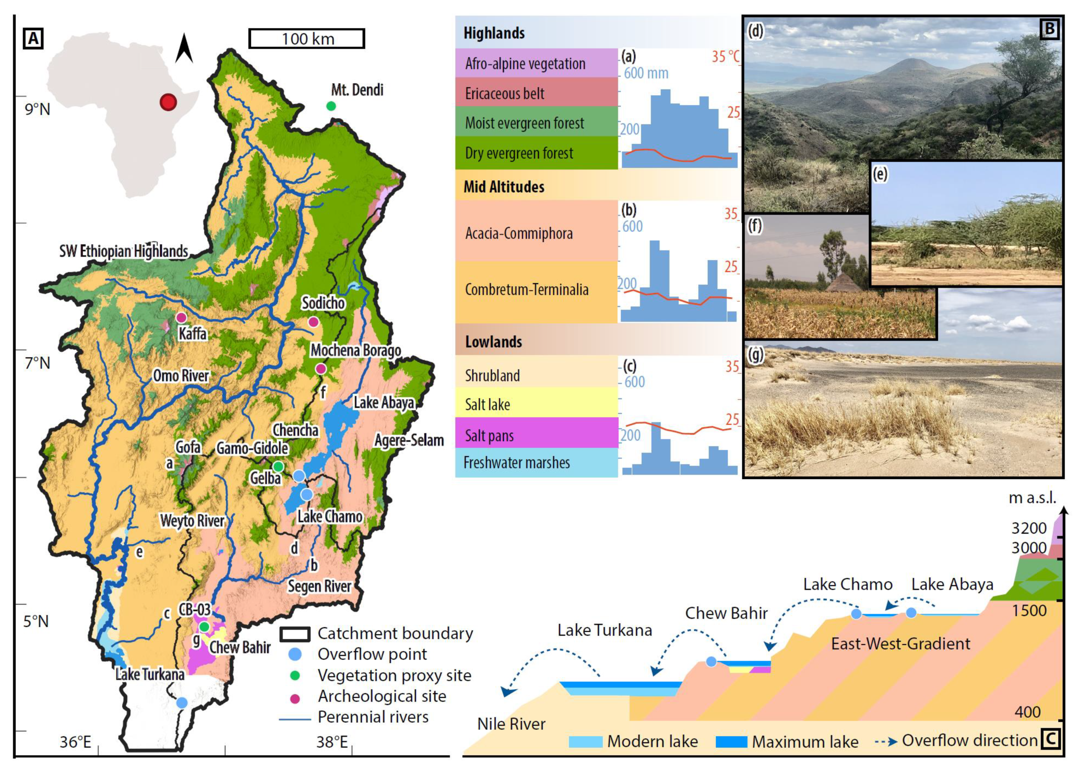
2. Regional Setting
2.1. Geology, Hydrology and Climate
2.2. Vegetation
2.3. Overview of Archaeological Records of the Last 25 ka in Ethiopia
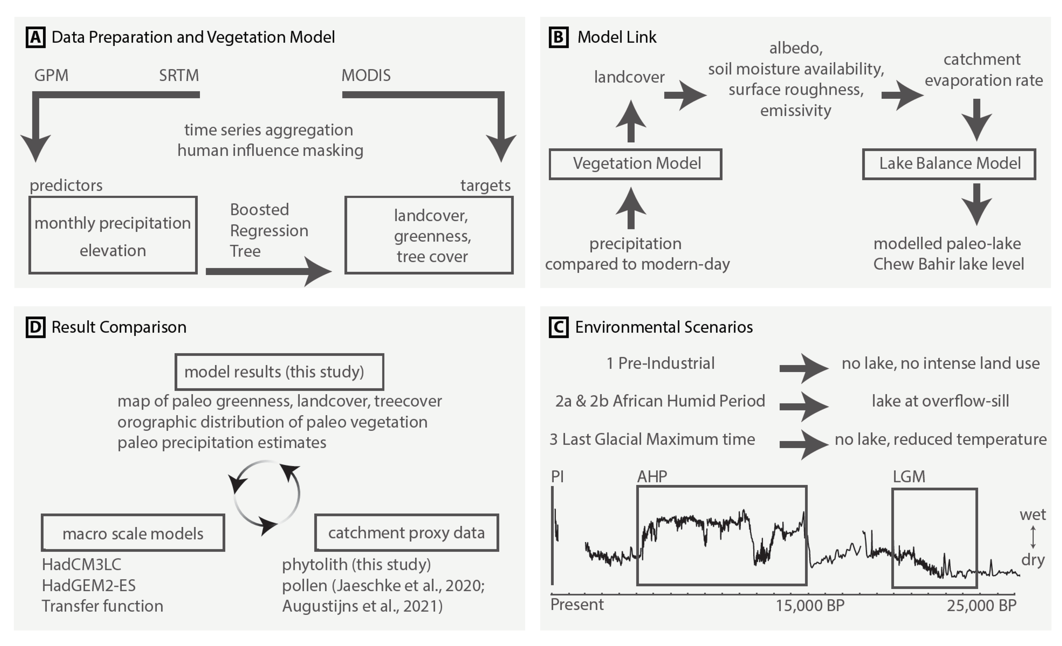
3. Materials and Methods
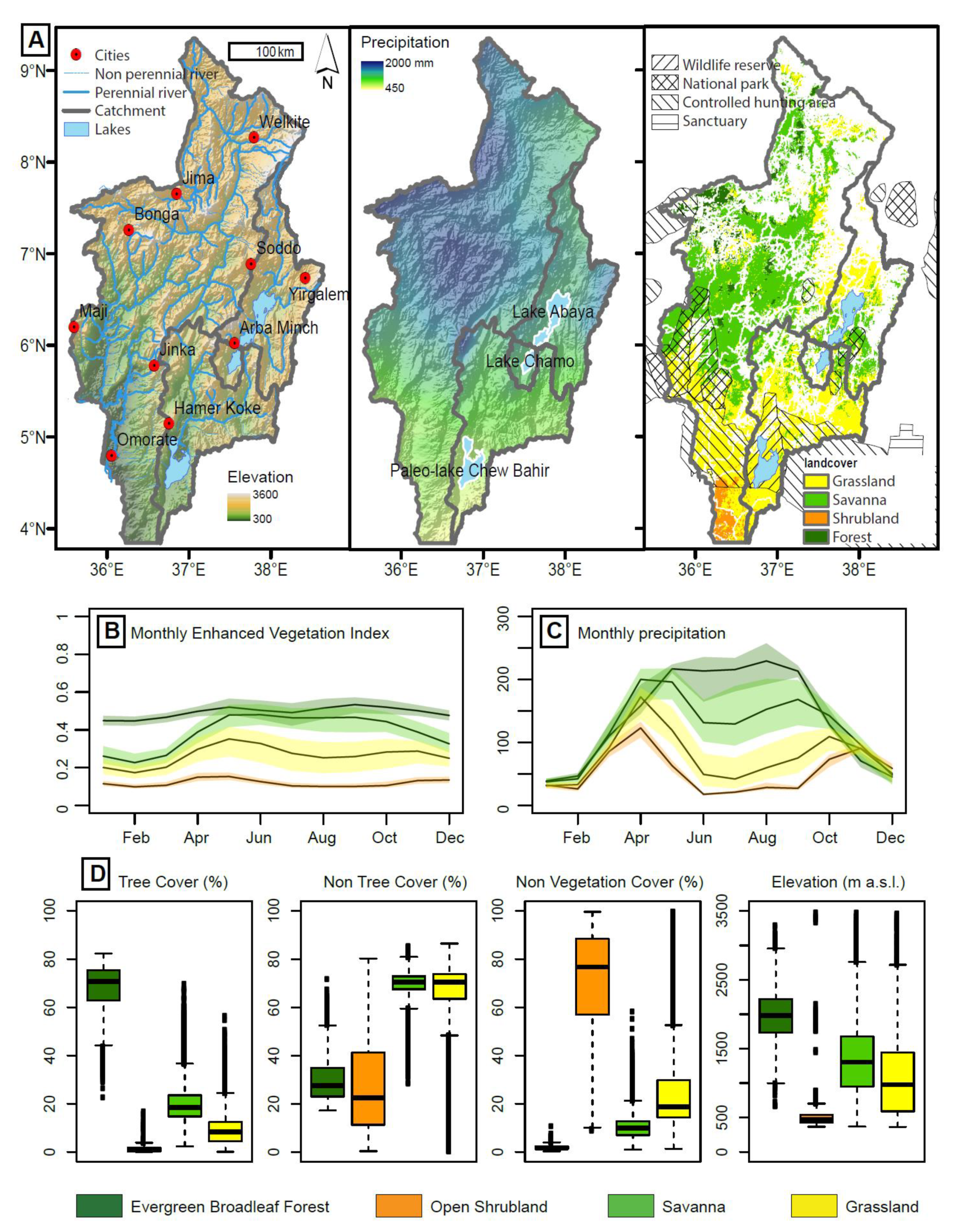
3.1. Training and Prediction Data
3.2. Model Training and Validation
3.3. Model Link and Scenarios
3.3.1. Stage 1—Precipitation to Vegetation
3.3.2. Stage 2—Vegetation to ET
3.3.3. Stage 3—ET to Lake Levels and Paleo-Precipitation
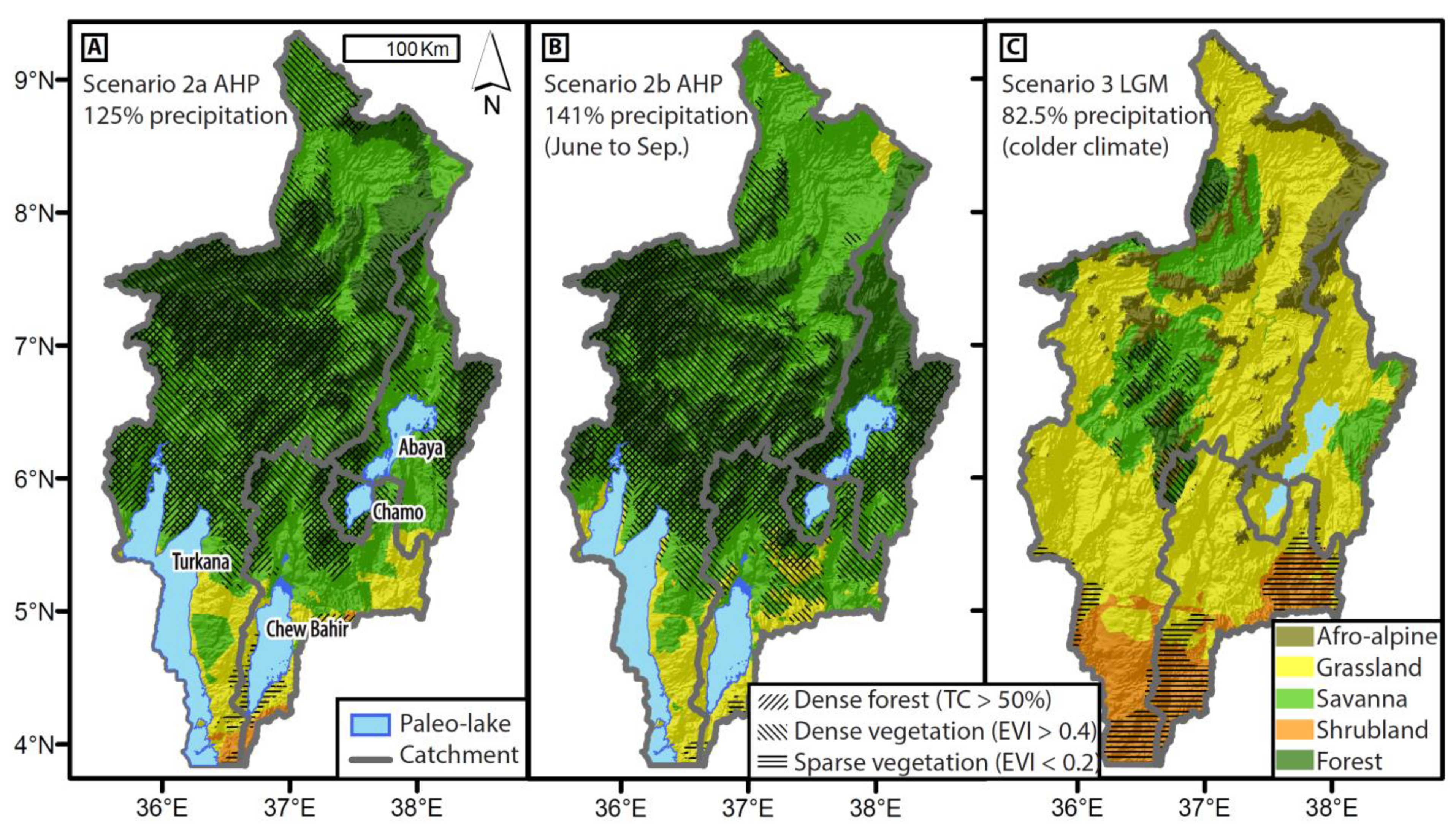
3.3.4. Paleo-Vegetation Maps
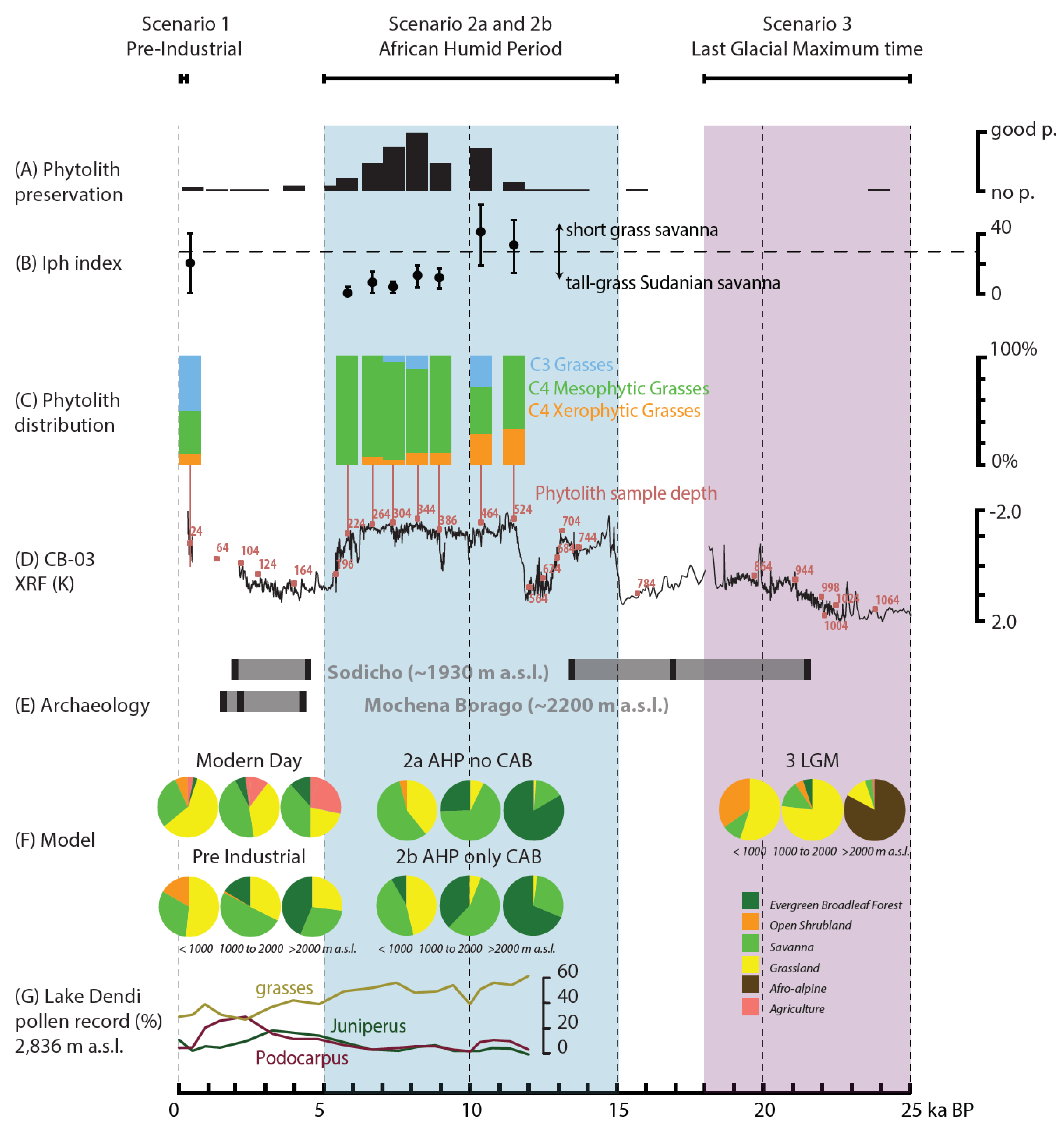
3.4. Phytolith Proxy
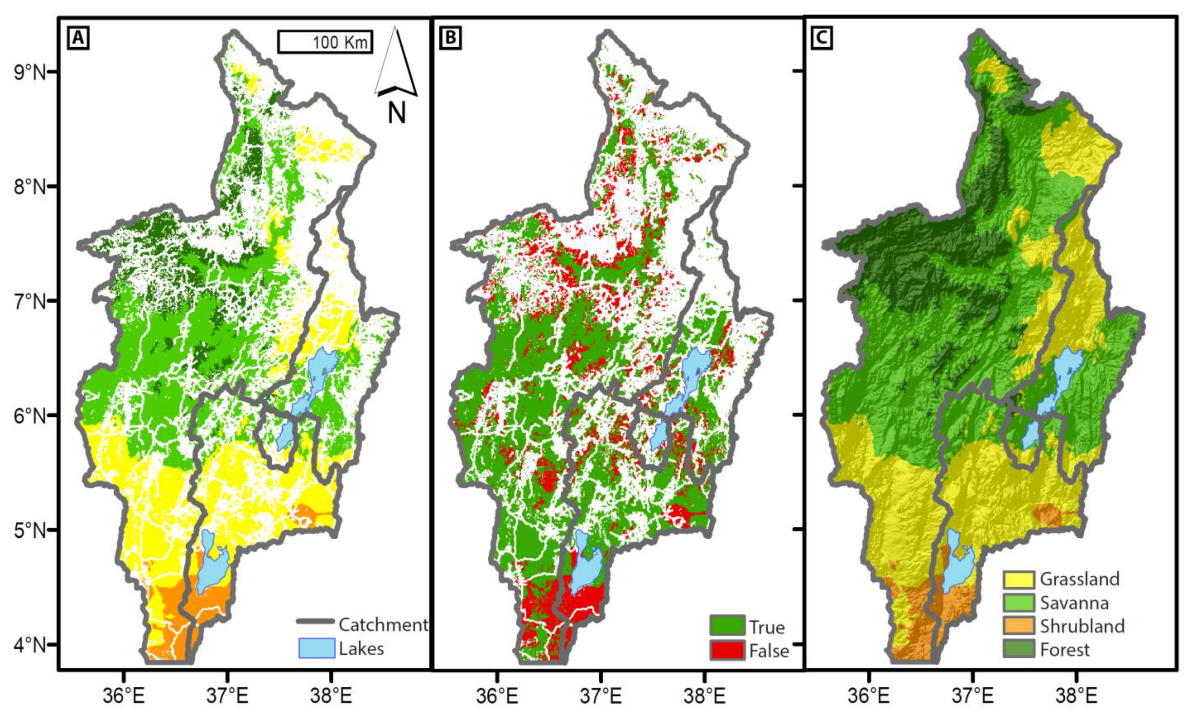
4. Results
4.1. Dataset Exploration and Description
4.2. Model Training and Validation
4.3. Model Link and Scenarios
4.3.1. Modern-Day and Pre-Industrial LC and ET
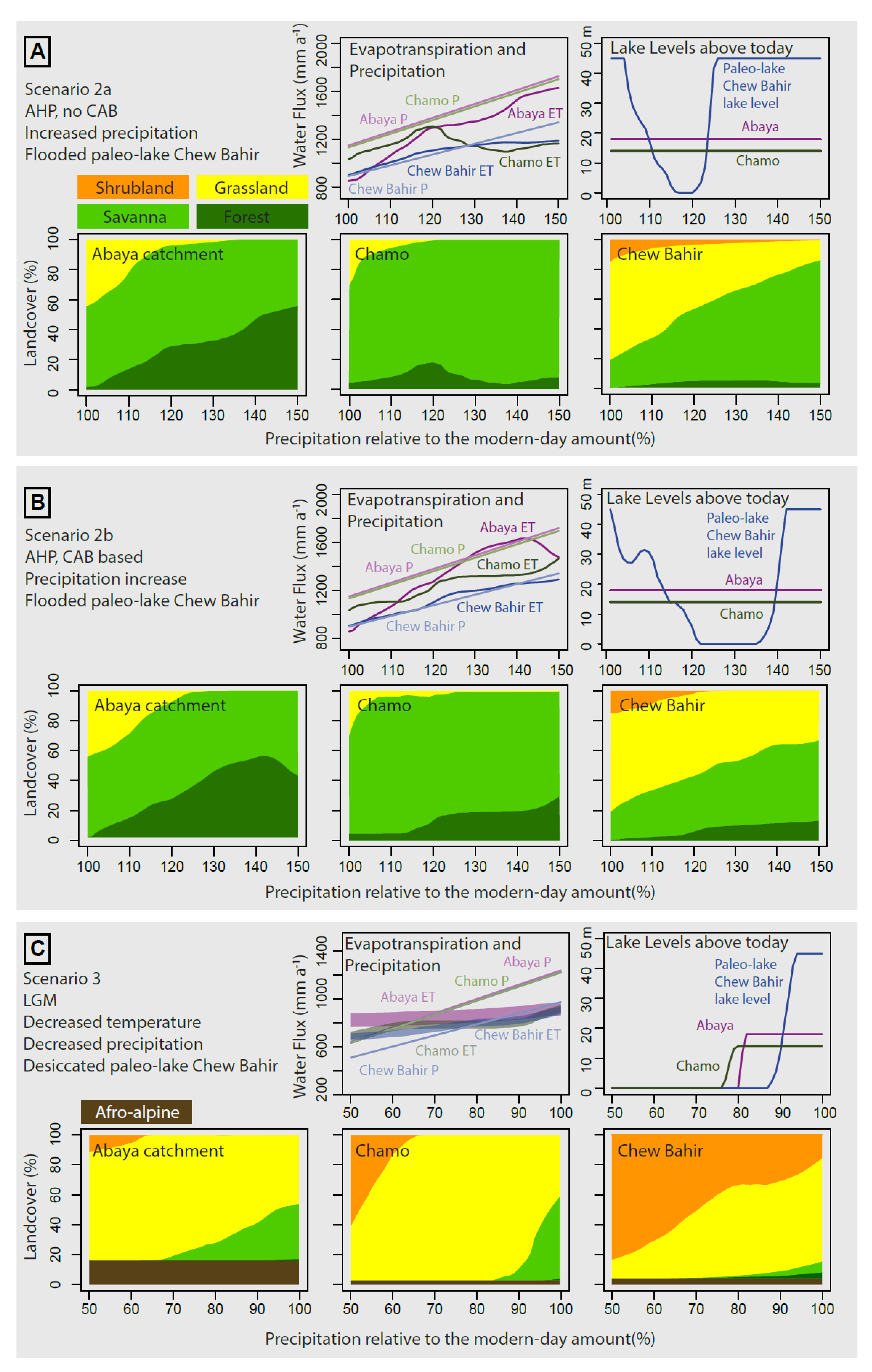
4.3.2. Scenario 2a—AHP, no CAB
4.3.3. Scenario 2b—AHP, with CAB
4.3.4. Scenario 3—LGM
4.3.5. PVM and LBM Model Link
4.4. Phytolith Proxy
5. Discussion
5.1. Results Synthesis
5.1.1. Scenario 3—LGM
5.1.2. Scenario 2—AHP
5.1.3. Scenario 1—Pre-Industrial
5.2. Proxy Model Interference
5.3. Limitations and Advantages of the Method
5.4. Human Landscape Preferences
6. Conclusions
Author Contributions
Funding
Institutional Review Board Statement
Informed Consent Statement
Data Availability Statement
Acknowledgments
Conflicts of Interest
References
- Corti, G. Continental rift evolution: From rift initiation to incipient break-up in the Main Ethiopian Rift, East Africa. Earth Sci. Rev. 2009, 96, 1–53. [Google Scholar] [CrossRef]
- Nicholson, S.E. Climate and climatic variability of rainfall over eastern Africa. Rev. Geophys. 2017, 55, 590–635. [Google Scholar] [CrossRef] [Green Version]
- Friis, I.; Demissew, S.; van Breugel, P. Atlas of the Potential Vegetation of Ethiopia; Det Kongelige Danske Videnskabernes Selskab: Copenhagen, Denmark, 2011. [Google Scholar]
- Schaebitz, F.; Asrat, A.; Lamb, H.F.; Cohen, A.S.; Foerster, V.; Duesing, W.; Kaboth-Bahr, S.; Opitz, S.; Viehberg, F.A.; Vogelsang, R.; et al. Hydroclimate changes in eastern Africa over the past 200,000 years may have influenced early human dispersal. Commun. Earth Environ. 2021, 2, 123. [Google Scholar] [CrossRef]
- Kaboth-Bahr, S.; Gosling, W.D.; Vogelsang, R.; Bahr, A.; Scerri, E.M.L.; Asrat, A.; Cohen, A.S.; Düsing, W.; Foerster, V.; Lamb, H.F.; et al. Paleo-ENSO influence on African environments and early modern humans. Proc. Nat. Acad. Sci. USA 2021, 118, e2018277118. [Google Scholar] [CrossRef]
- Gasse, F. Hydrological changes in the african tropics since the last glacial maximum. Quat. Sci. Rev. 2000, 19, 189–211. [Google Scholar] [CrossRef]
- Loomis, S.E.; Russell, J.M.; Verschuren, D.; Morrill, C.; De Cort, G.; Sinninghe Damsté, J.S.; Olago, D.; Eggermont, H.; Street-Perrott, F.A.; Kelly, M.A. The tropical lapse rate steepened during the Last Glacial Maximum. Sci. Adv. 2017, 3, e1600815. [Google Scholar] [CrossRef] [Green Version]
- Barker, P.A.; Talbot, M.R.; Street-Perrott, F.A.; Marret, F.; Scourse, J.; Odada, E.O. Late quaternary climatic variability in intertropical Africa. In Past Climate Variability through Europe and Africa; Springer: Berlin, Germany, 2004; pp. 117–138. [Google Scholar]
- Demenocal, P.; Ortiz, J.; Guilderson, T.; Adkins, J.; Sarnthein, M.; Baker, L.; Yarusinsky, M. Abrupt onset and termination of the African humid period. Quat. Sci. Rev. 2000, 19, 347–361. [Google Scholar] [CrossRef]
- Fischer, M.L.; Markowska, M.; Bachofer, F.; Foerster, V.E.; Asrat, A.; Zielhofer, C.; Trauth, M.H.; Junginger, A. Determining the pace and magnitude of lake level changes in Southern Ethiopia over the last 20,000 years using lake balance modeling and SEBAL. Front. Earth Sci. 2020, 8, 197. [Google Scholar] [CrossRef]
- Foerster, V.; Junginger, A.; Langkamp, O.; Gebru, T.; Asrat, A.; Umer, M.; Lamb, H.F.; Wennrich, V.; Rethemeyer, J.; Nowaczyk, N.; et al. Climatic change recorded in the sediments of the Chew Bahir basin, southern Ethiopia, during the last 45,000 years. Quat. Int. 2012, 274, 25. [Google Scholar] [CrossRef]
- Garcin, Y.; Melnick, D.; Strecker, M.R.; Olago, D.; Tiercelin, J.-J. East African mid-Holocene wet–dry transition recorded in palaeo-shorelines of Lake Turkana, northern Kenya Rift. Earth Planet. Sci. Lett. 2012, 331, 322–334. [Google Scholar] [CrossRef]
- Junginger, A.; Trauth, M.H. Hydrological constraints of paleo-Lake Suguta in the Northern Kenya Rift during the African Humid Period (15–5kaBP). Glob. Planet. Change 2013, 111, 174–188. [Google Scholar] [CrossRef]
- Costa, K.; Russell, J.; Konecky, B.; Lamb, H. Isotopic reconstruction of the African Humid Period and Congo Air Boundary migration at Lake Tana, Ethiopia. Quat. Sci. Rev. 2014, 83, 58–67. [Google Scholar] [CrossRef] [Green Version]
- Anhuf, D.; Ledru, M.P.; Behling, H.; Da Cruz, F.W.; Cordeiro, R.C.; Van der Hammen, T.; Karmann, I.; Marengo, J.A.; De Oliveira, P.E.; Pessenda, L.; et al. Paleo-environmental change in Amazonian and African rainforest during the LGM. Palaeogeogr. Palaeoclimatol. Palaeoecol. 2006, 239, 510–527. [Google Scholar] [CrossRef]
- Jaeschke, A.; Thienemann, M.; Schefuß, E.; Urban, J.; Schäbitz, F.; Wagner, B.; Rethemeyer, J. Holocene hydroclimate variability and vegetation response in the Ethiopian highlands (Lake Dendi). Front. Earth Sci. 2020, 8, 585770. [Google Scholar] [CrossRef]
- Lamb, A.L.; Leng, M.J.; Umer Mohammed, M.; Lamb, H.F. Holocene climate and vegetation change in the Main Ethiopian Rift Valley, inferred from the composition (C/N and δ13C) of lacustrine organic matter. Quat. Sci. Rev. 2004, 23, 881–891. [Google Scholar] [CrossRef]
- Umer, M.; Lamb, H.F.; Bonnefille, R.; Lézine, A.M.; Tiercelin, J.J.; Gibert, E.; Cazet, J.P.; Watrin, J. Late pleistocene and holocene vegetation history of the Bale Mountains, Ethiopia. Quat. Sci. Rev. 2007, 26, 2229–2246. [Google Scholar] [CrossRef]
- Darwin, C. The descent of man, and selection in relation to sex. Lond. Murray 1871, 415, 1871. [Google Scholar]
- Dart, R. Australopithecus africanus the man-ape of South Africa. S. Afr. J. Sci. 1925, 115, 195–199. [Google Scholar] [CrossRef] [Green Version]
- Falk, J.H.; Balling, J.D. Evolutionary influence on human landscape preference. Environ. Behav. 2010, 42, 479–493. [Google Scholar] [CrossRef]
- Tveit, M.S.; Ode Sang, Å.; Hagerhall, C.M. Scenic beauty: Visual landscape assessment and human landscape perception. Environ. Psychol. Introd. 2018, 45–54. [Google Scholar] [CrossRef]
- Niang, K.; Blinkhorn, J.; Ndiaye, M. The oldest Stone Age occupation of coastal West Africa and its implications for modern human dispersals: New insight from Tiémassas. Quat. Sci. Rev. 2018, 188, 167–173. [Google Scholar] [CrossRef]
- Shipton, C.; Blinkhorn, J.; Archer, W.; Kourampas, N.; Roberts, P.; Prendergast, M.E.; Curtis, R.; Herries, A.I.R.; Ndiema, E.; Boivin, N.; et al. The Middle to Later Stone Age transition at Panga ya Saidi, in the tropical coastal forest of eastern Africa. J. Hum. Evolut. 2021, 153, 102954. [Google Scholar] [CrossRef]
- Shipton, C.; Roberts, P.; Archer, W.; Armitage, S.J.; Bita, C.; Blinkhorn, J.; Courtney-Mustaphi, C.; Crowther, A.; Curtis, R.; Errico, F.D.; et al. 78,000-year-old record of Middle and Later Stone Age innovation in an East African tropical forest. Nat. Commun. 2018, 9, 1832. [Google Scholar]
- Roberts, P.; Prendergast, M.E.; Janzen, A.; Shipton, C.; Blinkhorn, J.; Zech, J.; Crowther, A.; Sawchuk, E.A.; Stewart, M.; Ndiema, E. Late Pleistocene to Holocene human palaeoecology in the tropical environments of coastal eastern Africa. Palaeogeogr. Palaeoclimatol. Palaeoecol. 2020, 537, 109438. [Google Scholar] [CrossRef]
- Faith, J.T.; Tryon, C.A.; Peppe, D.J.; Beverly, E.J.; Blegen, N.; Blumenthal, S.; Chritz, K.L.; Driese, S.G.; Patterson, D. Paleoenvironmental context of the Middle Stone Age record from Karungu, Lake Victoria Basin, Kenya, and its implications for human and faunal dispersals in East Africa. J. Hum. Evolut. 2015, 83, 28–45. [Google Scholar] [CrossRef] [Green Version]
- Wilkins, J.; Schoville, B.J.; Pickering, R.; Gliganic, L.; Collins, B.; Brown, K.S.; von der Meden, J.; Khumalo, W.; Meyer, M.C.; Maape, S. Innovative Homo sapiens behaviours 105,000 years ago in a wetter Kalahari. Nature 2021, 592, 248–252. [Google Scholar] [CrossRef] [PubMed]
- Ossendorf, G.; Groos, A.R.; Bromm, T.; Tekelemariam, M.G.; Glaser, B.; Lesur, J.; Schmidt, J.; Akçar, N.; Bekele, T.; Beldados, A.; et al. Middle Stone Age foragers resided in high elevations of the glaciated Bale Mountains, Ethiopia. Science 2019, 365, 583–587. [Google Scholar] [CrossRef]
- Vogelsang, R.; Bubenzer, O.; Kehl, M.; Meyer, S.; Richter, J.; Zinaye, B. When hominins conquered highlands—An acheulean site at 3000 m asl on mount dendi/Ethiopia. J. Paleolit. Archaeol. 2018, 1, 302–313. [Google Scholar] [CrossRef]
- Bergström, A.; Stringer, C.; Hajdinjak, M.; Scerri, E.M.L.; Skoglund, P. Origins of modern human ancestry. Nature 2021, 590, 229–237. [Google Scholar] [CrossRef]
- Nicholson, S.L.; Hosfield, R.; Groucutt, H.S.; Pike, A.W.G.; Fleitmann, D. Beyond arrows on a map: The dynamics of Homo sapiens dispersal and occupation of Arabia during Marine Isotope Stage 5. J. Anthropol. Archaeol. 2021, 62, 101269. [Google Scholar] [CrossRef]
- Foerster, V.; Vogelsang, R.; Junginger, A.; Asrat, A.; Lamb, H.F.; Schaebitz, F.; Trauth, M.H. Environmental change and human occupation of southern Ethiopia and northern Kenya during the last 20,000 years. Quat. Sci. Rev. 2015, 129, 333–340. [Google Scholar] [CrossRef] [Green Version]
- Junginger, A.; Roller, S.; Olaka, L.A.; Trauth, M.H. The effects of solar irradiation changes on the migration of the Congo Air Boundary and water levels of paleo-Lake Suguta, Northern Kenya Rift, during the African Humid Period (15–5ka BP). Palaeogeogr. Palaeoclimatol. Palaeoecol. 2014, 396, 1–16. [Google Scholar] [CrossRef]
- Beck, C.C.; Feibel, C.S.; Wright, J.D.; Mortlock, R.A. Onset of the African Humid Period by 13.9 kyr BP at Kabua Gorge, Turkana Basin, Kenya. Holocene 2019, 29, 1011–1019. [Google Scholar] [CrossRef] [Green Version]
- Bergner, A.G.N.; Trauth, M.H.; Bookhagen, B. Paleoprecipitation estimates for the Lake Naivasha basin (Kenya) during the last 175 k.y. using a lake-balance model. Glob. Planet. Change 2003, 36, 117–136. [Google Scholar] [CrossRef]
- Elith, J.; Graham, C.H.; Anderson, R.P.; Dudík, M.; Ferrier, S.; Guisan, A.; Hijmans, R.J.; Huettmann, F.; Leathwick, J.R.; Lehmann, A.; et al. Novel methods improve prediction of species′ distributions from occurrence data. Ecography 2006, 29, 129–151. [Google Scholar] [CrossRef] [Green Version]
- Guisan, A.; Zimmermann, N.E. Predictive habitat distribution models in ecology. Ecol. Model. 2000, 135, 147–186. [Google Scholar] [CrossRef]
- Van Breugel, P.; Friis, I.; Demissew, S.; Wesche, K. The transitional semi-evergreen bushland in Ethiopia: Characterization and mapping of its distribution using predictive modelling. Appl. Veg. Sci. 2016, 19, 355–367. [Google Scholar] [CrossRef]
- Guisan, A.; Edwards, T.C.; Hastie, T. Generalized linear and generalized additive models in studies of species distributions: Setting the scene. Ecol. Model. 2002, 157, 89–100. [Google Scholar] [CrossRef] [Green Version]
- Duque-Lazo, J.; Van Gils, H.; Groen, T.A.; Navarro-Cerrillo, R.M. Transferability of species distribution models: The case of Phytophthora cinnamomi in Southwest Spain and Southwest Australia. Ecol. Model. 2016, 320, 62–70. [Google Scholar] [CrossRef]
- Pearson, R.G.; Dawson, T.P. Predicting the impacts of climate change on the distribution of species: Are bioclimate envelope models useful? Glob. Ecol. Biogeogr. 2003, 12, 361–371. [Google Scholar] [CrossRef] [Green Version]
- Termansen, M.; Mcclean, C.J.; Preston, C.D. The use of genetic algorithms and Bayesian classification to model species distributions. Ecol. Model. 2006, 192, 410–424. [Google Scholar] [CrossRef]
- Drake, J.M.; Lodge, D.M. Allee effects, propagule pressure and the probability of establishment: Risk analysis for biological invasions. Biol. Invasions 2006, 8, 365–375. [Google Scholar] [CrossRef]
- Fukuda, S.; De Baets, B.; Waegeman, W.; Verwaeren, J.; Mouton, A.M. Habitat prediction and knowledge extraction for spawning European grayling (Thymallus thymallus L.) using a broad range of species distribution models. Environ. Model. Softw. 2013, 47, 84. [Google Scholar] [CrossRef]
- Rammer, W.; Seidl, R. A scalable model of vegetation transitions using deep neural networks. Methods Ecol. Evol. 2019, 10, 879–890. [Google Scholar] [CrossRef] [Green Version]
- Elith, J.; Leathwick, J.R.; Hastie, T. A working guide to boosted regression trees. J. Anim. Ecol. 2008, 77, 802–813. [Google Scholar] [CrossRef]
- Kleinbauer, I.; Dullinger, S.; Peterseil, J.; Essl, F. Climate change might drive the invasive tree Robinia pseudacacia into nature reserves and endangered habitats. Biol. Conserv. 2010, 143, 382–390. [Google Scholar] [CrossRef]
- Mohr, P.; Zanettin, B. The Ethiopian flood basalt province. In Continental Flood Basalts; Springer: Berlin, Germany, 1988; pp. 63–110. [Google Scholar]
- Johnson, T.C.; Malala, J.O. Lake Turkana and its link to the Nile. In The Nile; Springer: Berlin, Germany, 2009; pp. 287–304. [Google Scholar]
- Segele, Z.T.; Lamb, P.J. Characterization and variability of Kiremt rainy season over Ethiopia. Meteorol. Atmos. Phys. 2005, 89, 153–180. [Google Scholar] [CrossRef]
- Asefa, M.; Cao, M.; He, Y.; Mekonnen, E.; Song, X.; Yang, J. Ethiopian vegetation types, climate and topography. Plant Divers. 2020, 42, 302–311. [Google Scholar] [CrossRef]
- Hedberg, O. Features of Afroalpine Plant Ecology; Sv. växtgeografiska sällsk: Upsala, Sweden, 1964. [Google Scholar]
- Bruhl, J.; Wilson, K. Towards a comprehensive survey of C3 and C4 photosynthetic pathways in Cyperaceae. Aliso 2007, 23, 99–148. [Google Scholar] [CrossRef] [Green Version]
- Brown, R.H.; Bouton, J.H.; Evans, P.T.; Malter, H.E.; Rigsby, L.L. Photosynthesis, morphology, leaf anatomy, and cytogenetics of hybrids between C3 and C3/C4Panicum species. Plant Physiol. 1985, 77, 653–658. [Google Scholar] [CrossRef] [PubMed] [Green Version]
- Leplongeon, A.; Pleurdeau, D.; Hovers, E. Late Pleistocene and Holocene Lithic variability at Goda Buticha (Southeastern Ethiopia): Implications for the understanding of the Middle and Late Stone Age of the Horn of Africa. J. Afr. Archaeol. 2017, 15, 202–233. [Google Scholar] [CrossRef]
- Tribolo, C.; Asrat, A.; Bahain, J.-J.; Chapon, C.; Douville, E.; Fragnol, C.; Hernandez, M.; Hovers, E.; Leplongeon, A.; Martin, L.; et al. Across the gap: Geochronological and sedimentological analyses from the late Pleistocene-Holocene sequence of Goda Buticha, Southeastern Ethiopia. PLoS ONE 2017, 12, e0169418. [Google Scholar] [CrossRef] [PubMed] [Green Version]
- Pleurdeau, D.; Hovers, E.; Assefa, Z.; Asrat, A.; Pearson, O.; Bahain, J.-J.; Lam, Y.M. Cultural change or continuity in the late MSA/Early LSA of southeastern Ethiopia? The site of Goda Buticha, Dire Dawa area. Quat. Int. 2014, 343, 117–135. [Google Scholar] [CrossRef]
- Brandt, S.A.; Fisher, E.C.; Hildebrand, E.A.; Vogelsang, R.; Ambrose, S.H.; Lesur, J.; Wang, H. Early MIS 3 occupation of Mochena Borago Rockshelter, Southwest Ethiopian Highlands: Implications for Late Pleistocene archaeology, paleoenvironments and modern human dispersals. Quat. Int. 2012, 274, 38–54. [Google Scholar] [CrossRef]
- Brandt, S.; Hildebrand, E.; Vogelsang, R.; Wolfhagen, J.; Wang, H. A new MIS 3 radiocarbon chronology for Mochena Borago Rockshelter, SW Ethiopia: Implications for the interpretation of Late Pleistocene chronostratigraphy and human behavior. J. Archaeol. Sci. Rep. 2017, 11, 352–369. [Google Scholar] [CrossRef] [Green Version]
- Ménard, C.; Bon, F.; Dessie, A.; Bruxelles, L.; Douze, K.; Fauvelle, F.-X.; Khalidi, L.; Lesur, J.; Mensan, R. Late Stone Age variability in the Main Ethiopian Rift: New data from the Bulbula River, Ziway–Shala basin. Quat. Int. 2014, 343, 53–68. [Google Scholar] [CrossRef]
- Leplongeon, A. Microliths in the Middle and Later Stone Age of eastern Africa: New data from Porc-Epic and Goda Buticha cave sites, Ethiopia. Quat. Int. 2014, 343, 100–116. [Google Scholar] [CrossRef]
- Assefa, Z. Faunal remains from Porc-Epic: Paleoecological and zooarchaeological investigations from a Middle Stone Age site in southeastern Ethiopia. J. Hum. Evol. 2006, 51, 50–75. [Google Scholar] [CrossRef]
- Hensel, E.A.; Vogelsang, R.; Noack, T.; Bubenzer, O. Stratigraphy and chronology of Sodicho Rockshelter—A new sedimentological record of past environmental changes and human settlement phases in Southwestern Ethiopia. Front. Earth Sci. 2021, 8, 640. [Google Scholar] [CrossRef]
- Khalidi, L.; Mologni, C.; Ménard, C.; Coudert, L.; Gabriele, M.; Davtian, G.; Cauliez, J.; Lesur, J.; Bruxelles, L.; Chesnaux, L.; et al. 9000 years of human lakeside adaptation in the Ethiopian Afar: Fisher-foragers and the first pastoralists in the Lake Abhe basin during the African Humid Period. Quat. Sci. Rev. 2020, 243, 106459. [Google Scholar] [CrossRef]
- Bachechi, L. Notizie preliminari sulla campagna di scavo 2002 svolta nel deposito del riparo di Harurona. CAVANNA C. A Cura di, Wolayta, una Regione d’Etiopia. Studi e Ricerche 1995, 2004, 67–78. [Google Scholar]
- Gossa, T.; Sahle, Y.; Negash, A. A reassessment of the Middle and Later Stone Age lithic assemblages from Aladi Springs, Southern Afar Rift, Ethiopia. Azania Archaeol. Res. Afr. 2012, 47, 210–222. [Google Scholar] [CrossRef]
- Williams, M.A.J.; Bishop, P.M.; Dakin, F.M.; Gillespie, R. Late quaternary lake levels in southern Afar and the adjacent Ethopian Rift. Nature 1977, 267, 690–693. [Google Scholar] [CrossRef]
- Kurashina, H. An Examination of Prehistoric Lithic Technology in East-Central Ethiopia; University of California, Berkeley: Berkeley, CA, USA, 1978. [Google Scholar]
- Finneran, N.; Boardman, S.; Cain, C. Excavations at the Late Stone Age Site of Baahti Nebait, Aksum, Northern Ethiopia, 1997. AZANIA J. Br. Inst. East. Afr. 2000, 35, 53–73. [Google Scholar] [CrossRef]
- Ashkenazy, H.; Sahle, Y. An early Holocene Lithic assemblage from Dibé Rockshelter, South-Central Ethiopia. J. Afr. Archaeol. 2021, 1, 1–15. [Google Scholar] [CrossRef]
- Arthur, J.W.; Curtis, M.C.; Arthur, K.J.W.; Coltorti, M.; Pieruccini, P.; Lesur, J.; Fuller, D.; Lucas, L.; Conyers, L.; Stock, J.; et al. The transition from hunting–gathering to food production in the Gamo Highlands of Southern Ethiopia. Afr. Archaeol. Rev. 2019, 36, 5–65. [Google Scholar] [CrossRef] [Green Version]
- Hildebrand, E.A.; Brandt, S.A.; Lesur-Gebremariam, J. The holocene archaeology of Southwest Ethiopia: New insights from the Kafa Archaeological project. Afr. Archaeol. Rev. 2010, 27, 255–289. [Google Scholar] [CrossRef]
- Schepers, C.; Lesur, J.; Vogelsang, R. Hunter-gatherers of the high-altitude Afromontane forest—The Holocene occupation of Mount Dendi, Ethiopia. Azania Archaeol. Res. Afr. 2020, 55, 329–359. [Google Scholar] [CrossRef]
- Rowntree, P. Atmospheric parameterization schemes for evaporation over land: Basic concepts and climate modeling aspects. In Land Surface Evaporation; Springer: Berlin, Germany, 1991; pp. 5–29. [Google Scholar]
- Farr, T.G.; Rosen, P.A.; Caro, E.; Crippen, R.; Duren, R.; Hensley, S.; Kobrick, M.; Paller, M.; Rodriguez, E.; Roth, L.; et al. The shuttle radar topography mission. Rev. Geophys. 2007, 45, 1–33. [Google Scholar] [CrossRef] [Green Version]
- Huffman, G.J.; Stocker, E.F.; Bolvin, D.T.; Nelkin, E.J.; Tan, J. GPM IMERG Final Precipitation L3 1 Month 0.1 Degree x 0.1 Degree V06; Goddard Earth Sciences Data and Information Services Center (GES DISC): Greenbelt, MD, USA, 2019. [Google Scholar]
- Friedl, M.; Sulla-Menashe, D. MCD12Q1 MODIS/Terra+Aqua Land Cover Type Yearly L3 Global 500m SIN Grid V006 (Data Set); NASA EOSDIS Land Processes DAAC: Sioux Falls, SD, USA, 2019. [Google Scholar] [CrossRef]
- DiMiceli, C.; Carroll, M.; Sohlberg, R.; Kim, D.; Kelly, M.; Townshend, J. MOD44B MODIS/Terra Vegetation Continuous Fields Yearly L3 Global 250m SIN Grid V006 (Data Set); NASA EOSDIS Land Processes DAAC: Sioux Falls, SD, USA, 2015. [Google Scholar] [CrossRef]
- Didan, K. MOD13A3 MODIS/Terra Vegetation Indices Monthly L3 Global 1km SIN Grid V006 (Data Set); NASA EOSDIS Land Processes DAAC: Sioux Falls, SD, USA, 2015. [Google Scholar] [CrossRef]
- R Core Team, R. A Language and Environment for Statistical Computing; R Foundation for Statistical Computing: Vienna, Austria, 2021. [Google Scholar]
- Hijmans, R.J. raster: Geographic Data Analysis and Modeling, R package version 3.1-5; 2020. [Google Scholar]
- Bivand, R.; Keitt, T.; Rowlingson, B. rgdal: Bindings for the ‘Geospatial’ Data Abstraction Library, R package version 1.5-10; 2020. [Google Scholar]
- OpenStreetMap, C. Planet Dump. 2017. Available online: https://planet.osm.org (accessed on 1 March 2020).
- Friedl, M.A.; Sulla-Menashe, D.; Tan, B.; Schneider, A.; Ramankutty, N.; Sibley, A.; Huang, X. MODIS Collection 5 global land cover: Algorithm refinements and characterization of new datasets. Remote Sens. Environ. 2010, 114, 168–182. [Google Scholar] [CrossRef]
- Acker, J.G.; Leptoukh, G. Online analysis enhances use of NASA earth science data. Eos Trans. Am. Geophys. Union 2007, 88, 14–17. [Google Scholar] [CrossRef]
- Friedman, J.H. Greedy function approximation: A gradient boosting machine. Ann. Stat. 2001, 29, 1189–1232. [Google Scholar] [CrossRef]
- Greenwell, B.; Boehmke, B.; Cunningham, J.; Developers, G. gbm: Generalized Boosted Regression Models, R package version 2.1.5; 2019. [Google Scholar]
- Robin, X.; Turck, N.; Hainard, A.; Tiberti, N.; Lisacek, F.; Jean-Charles, S.; Müller, M. pROC: An open-source package for R and S+ to analyze and compare ROC curves. BMC Bioinform. 2011, 12, 77. [Google Scholar] [CrossRef]
- Kuhn, M. caret: Classification and Regression Training, R package version 6.0-86; 2020. [Google Scholar]
- Lyons, R.P.; Kroll, C.N.; Scholz, C.A. An energy-balance hydrologic model for the Lake Malawi Rift Basin, East Africa. Glob. Planet. Change 2011, 75, 83–97. [Google Scholar] [CrossRef]
- Loomis, S.E.; Russell, J.M.; Ladd, B.; Street-Perrott, F.A.; Sinninghe Damsté, J.S. Calibration and application of the branched GDGT temperature proxy on East African lake sediments. Earth Planet. Sci. Lett. 2012, 357, 277–288. [Google Scholar] [CrossRef]
- Foerster, V.; Deocampo, D.M.; Asrat, A.; Günter, C.; Junginger, A.; Krämer, K.H.; Stroncik, N.A.; Trauth, M.H. Towards an understanding of climate proxy formation in the Chew Bahir basin, southern Ethiopian Rift. Palaeogeogr. Palaeoclimatol. Palaeoecol. 2018, 501, 111–123. [Google Scholar] [CrossRef]
- Trauth, M.H.; Foerster, V.; Junginger, A.; Asrat, A.; Lamb, H.F.; Schaebitz, F. Abrupt or gradual? Change point analysis of the late Pleistocene–Holocene climate record from Chew Bahir, southern Ethiopia. Quat. Res. 2018, 90, 321–330. [Google Scholar] [CrossRef] [Green Version]
- Yost, C.L.; Ivory, S.J.; Deino, A.L.; Rabideaux, N.M.; Kingston, J.D.; Cohen, A.S. Phytoliths, pollen, and microcharcoal from the Baringo Basin, Kenya reveal savanna dynamics during the Plio-Pleistocene transition. Palaeogeogr. Palaeoclimatol. Palaeoecol. 2021, 570, 109779. [Google Scholar] [CrossRef]
- Piperno, D.R. Phytoliths: A Comprehensive Guide for Archaeologists and Paleoecologists; Rowman Altamira: Lanham, MD, USA, 2006. [Google Scholar]
- Li, R.; Fan, J.; Vachula, R.S.; Tan, S.; Qing, X. Spatial distribution characteristics and environmental significance of phytoliths in surface sediments of Qingshitan Lake in Southwest China. J. Paleolimnol. 2019, 61, 201–215. [Google Scholar] [CrossRef]
- Madella, M.; Alexandre, A.; Ball, T. International code for phytolith nomenclature 1.0. Ann. Bot. 2005, 96, 253–260. [Google Scholar] [CrossRef] [Green Version]
- Yost, C.L.; Lupien, R.L.; Beck, C.; Feibel, C.S.; Archer, S.R.; Cohen, A.S. Orbital influence on precipitation, fire, and grass community composition from 1.87 to 1.38 Ma in the Turkana Basin, Kenya. Front. Earth Sci. 2021, 9, 646. [Google Scholar] [CrossRef]
- Novello, A.; Barboni, D.; Sylvestre, F.; Lebatard, A.-E.; Paillès, C.; Bourlès, D.L.; Likius, A.; Mackaye, H.T.; Vignaud, P.; Brunet, M. Phytoliths indicate significant arboreal cover at Sahelanthropus type locality TM266 in northern Chad and a decrease in later sites. J. Hum. Evol. 2017, 106, 66–83. [Google Scholar] [CrossRef] [PubMed]
- Bremond, L.; Alexandre, A.; Peyron, O.; Guiot, J. Definition of grassland biomes from phytoliths in West Africa. J. Biogeogr. 2008, 35, 2039–2048. [Google Scholar] [CrossRef]
- Anhuf, D. Vegetation history and climate changes in Africa north and south of the equator (10 S to 10 N) during the last glacial maximum. In Southern Hemisphere Paleo-and Neoclimates; Springer: Berlin, Germany, 2000; pp. 225–248. [Google Scholar]
- Cowling, S.A.; Cox, P.M.; Jones, C.D.; Maslin, M.A.; Peros, M.; Spall, S.A. Simulated glacial and interglacial vegetation across Africa: Implications for species phylogenies and trans-African migration of plants and animals. Glob. Change Biol. 2008, 14, 827–840. [Google Scholar] [CrossRef]
- Hopcroft, P.O.; Valdes, P.J. Last glacial maximum constraints on the Earth system model HadGEM2-ES. Clim. Dyn. 2015, 45, 1657–1672. [Google Scholar] [CrossRef] [Green Version]
- Augustijns, F.; Broothaerts, N.; Verstraeten, G. Reconstructing vegetation changes in the Ethiopian Highlands: 18,000 years of Afromontane vegetation dynamics recorded in high altitude wetlands. In Proceedings of the EGU General Assembly Conference Abstracts, Vienna, Austria, 25–30 April 2021; p. EGU21-1340. [Google Scholar]
- Gillespie, R.; Street-Perrott, F.A.; Switsur, R. Post-glacial arid episodes in Ethiopia have implications for climate prediction. Nature 1983, 306, 680–683. [Google Scholar] [CrossRef]
- Hastenrath, S.; Kutzbach, J.E. Paleoclimatic estimates from water and energy budgets of East African lakes. Quat. Res. 1983, 19, 141–153. [Google Scholar] [CrossRef]
- Dühnforth, M.; Bergner, A.G.N.; Trauth, M.H. Early holocene water budget of the Nakuru-Elmenteita basin, Central Kenya Rift. J. Paleolimnol. 2006, 36, 281–294. [Google Scholar] [CrossRef] [Green Version]
- Darbyshire, I.; Lamb, H.; Umer, M. Forest clearance and regrowth in northern Ethiopia during the last 3000 years. Holocene 2003, 13, 537–546. [Google Scholar] [CrossRef]
- Nyssen, J.; Poesen, J.; Moeyersons, J.; Deckers, J.; Haile, M.; Lang, A. Human impact on the environment in the Ethiopian and Eritrean highlands—A state of the art. Earth Sci. Rev. 2004, 64, 273–320. [Google Scholar] [CrossRef]
- Gil-Romera, G.; Lamb, H.F.; Turton, D.; Sevilla-Callejo, M.; Umer, M. Long-term resilience, bush encroachment patterns and local knowledge in a Northeast African savanna. Glob. Environ. Change 2010, 20, 612–626. [Google Scholar] [CrossRef]
- Woldeyohannes, A.; Cotter, M.; Kelboro, G.; Dessalegn, W. Land use and land cover changes and their effects on the landscape of Abaya-Chamo Basin, Southern Ethiopia. Land 2018, 7, 2. [Google Scholar] [CrossRef] [Green Version]
- Von Höhnel, L. The Lake Rudolf region: Its discovery and subsequent exploration, 1888–1909. Part II. J. R. Afr. Soc. 1938, 37, 206–226. [Google Scholar]
- Nicholson, S.E. Climatic and environmental change in Africa during the last two centuries. Clim. Res. 2001, 17, 123–144. [Google Scholar] [CrossRef] [Green Version]
- Olaka, L.A. Hydrology Across Scales: Sensitivity of East African Lakes to Climate Changes; Universität Potsdam: Potsdam, Germany, 2011. [Google Scholar]
- Cabanes, D.; Weiner, S.; Shahack-Gross, R. Stability of phytoliths in the archaeological record: A dissolution study of modern and fossil phytoliths. J. Archaeol. Sci. 2011, 38, 2480–2490. [Google Scholar] [CrossRef]
- Greve, M.; Lykke, A.M.; Blach-Overgaard, A.; Svenning, J.-C. Environmental and anthropogenic determinants of vegetation distribution across Africa. Glob. Ecol. Biogeogr. 2011, 20, 661–674. [Google Scholar] [CrossRef]
- Hensel, E.A.; Bödeker, O.; Bubenzer, O.; Vogelsang, R. Combining geomorphological–hydrological analyses and the location of settlement and raw material sites—A case study on understanding prehistoric human settlement activity in the southwestern Ethiopian Highlands. E G Quat. Sci. J. 2019, 68, 201–213. [Google Scholar] [CrossRef]
- Basell, L. Middle Stone Age (MSA) site distributions in eastern Africa and their relationship to quaternary environmental change, refugia and the evolution of Homo sapiens. Quat. Sci. Rev. 2008, 27, 2484–2498. [Google Scholar] [CrossRef]
- Vogelsang, R.; Wendt, K.P. Reconstructing prehistoric settlement models and land use patterns on Mt. Damota/SW Ethiopia. Quat. Int. 2018, 485, 140–149. [Google Scholar] [CrossRef]
- Dekker, G.; Gebre Selassie, T. Rock engravings at Ch′ew Bahir. Ann. Ethiop. 1972, 9, 19. [Google Scholar] [CrossRef]
- Gutherz, X.; Jallot, L.; Lesur, J.; Pouzolles, G.; Sordoillet, D. Les fouilles de l′abri sous-roche de Moche Borago (Soddo, Wolyata). Premier bilan. Ann. Ethiop. 2002, 18, 181–190. [Google Scholar] [CrossRef]


| Data | Specification | Temporal Resolution | Spatial Resolution |
|---|---|---|---|
| Elevation | Shuttle Radar Topography Mission | - | ~90 m |
| Precipitation | Global Precipitation Measurement | Monthly | 0.1° |
| Landcover | MODIS, MCD12Q1, UMD | Annual | ~500 m |
| Greenness | MODIS, MOD13A3, EVI | Monthly | ~1000 m |
| Vegetation Cover | MODIS, MOD44B, VCF | Annual | ~250 m |
| UMD | Name | Albedo | Emissivity | SMA | Roughness Length (cm) |
|---|---|---|---|---|---|
| 0 | Water Bodies | 0.06 | 0.99 | 1 | 0.01 |
| 2 | Evergreen Broadleaf Forest | 0.07 | 0.96 | 0.5 | 50 |
| 6 | Closed Shrubland | 0.085 | 0.96 | 0.5 | 50 |
| 7 | Open Shrubland | 0.2 | 0.8 | 0.075 | 15 |
| 8 | Woody Savanna | 0.095 | 0.96 | 0.5 | 40 |
| 9 | Savanna | 0.13 | 0.96 | 0.18 | 25 |
| 10 | Grassland | 0.14 | 0.98 | 0.14 | 20 |
| 11 | Permanent Wetland | 0.055 | 1 | 0.8 | 0.01 |
| 12,14 | Cropland | 0.1 | 0.95 | 0.5 | 50 |
| 13 | Urban or Built-Up | 0.275 | 0.75 | 0.02 | 1 |
| 15 | Non vegetated | 0.25 | 0.75 | 0.02 | 1 |
| 16 | Afro-alpine | 0.125 | 0.97 | 0.5 | 27.5 |
| BRT | Distribution | Interaction Depth | Shrinkage | Bag Fraction | Trees | ROC/R2 |
|---|---|---|---|---|---|---|
| LC | multinomial | 1 | 0.05 | 0.5 | 298 | 0.79 |
| EVI | gaussian | 1 | 0.05 | 0.75 | 3096 | 0.8 |
| TC | gaussian | 3 | 0.05 | 0.5 | 1771 | 0.8 |
| NTC | gaussian | 5 | 0.05 | 0.5 | 3408 | 0.49 |
| NVC | gaussian | 3 | 0.05 | 0.5 | 2671 | 0.55 |
| Forest | Open Shrubland | Savanna | Grassland | |
|---|---|---|---|---|
| Forest | 2784 | 0 | 4313 | 1024 |
| Open Shrubland | 0 | 1198 | 4 | 4260 |
| Savanna | 237 | 1 | 23,289 | 4015 |
| Grassland | 14 | 839 | 2757 | 20,317 |
| Lake Abaya Catchment | Lake Chamo Catchment | Chew Bahir Catchment | ||||
|---|---|---|---|---|---|---|
| MD | PI | MD | PI | MD | PI | |
| Water | 6.1 | 6.1 | 15 | 15 | 0 | 0 |
| Forest | 1.2 | 1.8 | 0.1 | 4.5 | 0.2 | 0.6 |
| Open Shrubland | 0.1 | 0 | 0 | 0 | 0.6 | 14.5 |
| Savanna | 34 | 48 | 26.8 | 50.1 | 16.8 | 18.8 |
| Grassland | 37.3 | 44 | 44.9 | 30 | 75.2 | 62.2 |
| Cropland | 19 | 0 | 10.8 | 0 | 3.3 | 0 |
| Sparsely Vegetated | 0.5 | 0.5 | 0.4 | 0.4 | 3.9 | 3.9 |
| 1 | 4 | 24 | 64 | 104 | 124 | 164 | 196 | 224 | 264 | 304 | 344 | 386 | 464 | 524 | 564 | 624 | 684 | 704 | 744 | 784 | 864 | 944 | 998 | 1004 | 1024 | 1064 | 1098 |
| 2 | 98 | 242 | 200 | 336 | 329 | 141 | 155 | 51 | 7 | 19 | 17 | 34 | 18 | 227 | 150 | 346 | 355 | 43 | 298 | 295 | 267 | 203 | 272 | 294 | 289 | 273 | 286 |
| 3 | 9666 | 9666 | 9666 | 9666 | 9666 | 9666 | 9666 | 9666 | 9666 | 9666 | 9666 | 9666 | 9666 | 9666 | 9666 | 9666 | 9666 | 9666 | 9666 | 9666 | 9666 | 9666 | 9666 | 9666 | 9666 | 9666 | 9666 |
| 4 | 0.011 | 0.01 | 0.027 | 0.005 | 0.035 | 0.010 | 0.008 | 0.005 | 0.009 | 0.011 | 0.006 | 0.003 | 0.007 | 0.026 | 0.012 | 0.011 | 0.011 | −0.04 | 0.004 | 0.001 | 0 | 0.001 | 0.005 | 0.006 | 0.042 | 0.004 | 0.003 |
| 5 | 0 | 0 | 0 | 0 | 0 | 0 | 0 | 0 | 0 | 4 | 0 | 0 | 0 | 0 | 0 | 0 | 0 | 0 | 0 | 0 | 0 | 0 | 0 | 0 | 0 | 0 | 0 |
| 6 | 0 | 0 | 0 | 0 | 0 | 0 | 0 | 0 | 0 | 0 | 0 | 0 | 0 | 0 | 0 | 0 | 0 | 0 | 0 | 0 | 0 | 0 | 0 | 0 | 0 | 0 | 0 |
| 7 | 0 | 0 | 0 | 0 | 0 | 0 | 0 | 0 | 0 | 0 | 0 | 0 | 0 | 0 | 0 | 0 | 0 | 0 | 0 | 0 | 0 | 0 | 0 | 0 | 0 | 0 | 0 |
| 8 | 10 | 0 | 0 | 0 | 0 | 0 | 0 | 0 | 0 | 0 | 10 | 1 | 9 | 0 | 0 | 0 | 0 | 0 | 0 | 0 | 0 | 0 | 0 | 0 | 0 | 0 | 0 |
| 9 | 0 | 0 | 0 | 0 | 0 | 0 | 0 | 0 | 0 | 0 | 0 | 0 | 0 | 0 | 0 | 0 | 0 | 0 | 0 | 0 | 0 | 0 | 0 | 0 | 0 | 0 | 0 |
| 10 | 0 | 0 | 0 | 0 | 0 | 0 | 0 | 0 | 0 | 0 | 0 | 0 | 0 | 0 | 0 | 0 | 0 | 0 | 0 | 0 | 0 | 0 | 0 | 0 | 0 | 0 | |
| 11 | 0 | 0 | 0 | 0 | 0 | 0 | 0 | 0 | 0 | 0 | 0 | 0 | 0 | 0 | 0 | 0 | 0 | 0 | 0 | 0 | 0 | 0 | 0 | 0 | 0 | 0 | 0 |
| 12 | 10 | 0 | 0 | 0 | 0 | 0 | 0 | 0 | 0 | 4 | 10 | 1 | 9 | 0 | 0 | 0 | 0 | 0 | 0 | 0 | 0 | 0 | 0 | 0 | 0 | 0 | 0 |
| 13 | 2 | 0 | 0 | 0 | 0 | 0 | 0 | 0 | 2 | 4 | 9 | 7 | 9 | 1 | 0 | 0 | 0 | 0 | 0 | 0 | 0 | 0 | 0 | 0 | 0 | 0 | 0 |
| 14 | 0 | 0 | 0 | 0 | 0 | 0 | 0 | 0 | 0 | 0 | 0 | 0 | 0 | 0 | 0 | 0 | 0 | 0 | 0 | 0 | 0 | 0 | 0 | 0 | 0 | 0 | 0 |
| 15 | 2 | 0 | 0 | 0 | 0 | 0 | 0 | 0 | 2 | 4 | 9 | 7 | 9 | 1 | 0 | 0 | 0 | 0 | 0 | 0 | 0 | 0 | 0 | 0 | 0 | 0 | 0 |
| 16 | 0 | 0 | 0 | 0 | 0 | 0 | 0 | 0 | 0 | 0 | 0 | 0 | 0 | 0 | 0 | 0 | 0 | 0 | 0 | 0 | 0 | 0 | 0 | 0 | 0 | 0 | 0 |
| 17 | 0 | 0 | 0 | 0 | 0 | 0 | 0 | 17 | 0 | 33 | 10 | 9 | 8 | 0 | 0 | 0 | 0 | 0 | 0 | 0 | 0 | 0 | 0 | 0 | 0 | 0 | 0 |
| 18 | 6 | 0 | 0 | 0 | 0 | 0 | 0 | 0 | 7 | 0 | 0 | 0 | 0 | 0 | 0 | 0 | 0 | 0 | 0 | 0 | 0 | 1 | 0 | 0 | 0 | 0 | 0 |
| 19 | 0 | 0 | 0 | 0 | 0 | 0 | 0 | 0 | 0 | 4 | 0 | 1 | 0 | 0 | 0 | 0 | 0 | 0 | 0 | 0 | 0 | 0 | 0 | 0 | 0 | 0 | 0 |
| 20 | 2 | 0 | 0 | 0 | 0 | 1 | 0 | 30 | 19 | 54 | 58 | 51 | 5 | 2 | 0 | 0 | 0 | 0 | 0 | 0 | 0 | 1 | 0 | 0 | 0 | 0 | 0 |
| 21 | 2 | 0 | 0 | 0 | 0 | 1 | 0 | 30 | 19 | 58 | 58 | 52 | 5 | 2 | 0 | 0 | 0 | 0 | 0 | 0 | 0 | 1 | 0 | 0 | 0 | 0 | 0 |
| 22 | 6 | 0 | 0 | 0 | 0 | 0 | 0 | 17 | 7 | 33 | 10 | 9 | 8 | 0 | 0 | 0 | 0 | 0 | 0 | 0 | 0 | 1 | 0 | 0 | 0 | 0 | 0 |
| 23 | 8 | 0 | 0 | 0 | 0 | 1 | 0 | 47 | 26 | 91 | 68 | 61 | 13 | 2 | 0 | 0 | 0 | 0 | 0 | 0 | 0 | 2 | 0 | 0 | 0 | 0 | 0 |
| 24 | 0 | 0 | 0 | 0 | 0 | 0 | 0 | 17 | 0 | 0 | 0 | 1 | 0 | 0 | 0 | 0 | 0 | 0 | 0 | 0 | 0 | 0 | 0 | 0 | 0 | 0 | 0 |
| 25 | 0 | 0 | 0 | 0 | 0 | 0 | 0 | 0 | 0 | 0 | 0 | 0 | 0 | 0 | 0 | 0 | 0 | 0 | 0 | 0 | 0 | 0 | 0 | 0 | 0 | 0 | 0 |
| 26 | 0 | 0 | 0 | 0 | 0 | 0 | 0 | 26 | 1 | 0 | 5 | 0 | 4 | 0 | 0 | 0 | 0 | 1 | 0 | 0 | 0 | 2 | 0 | 0 | 0 | 0 | 0 |
| 27 | 0 | 0 | 0 | 0 | 0 | 0 | 0 | 0 | 0 | 0 | 0 | 0 | 0 | 0 | 0 | 0 | 0 | 0 | 0 | 0 | 0 | 0 | 0 | 0 | 0 | 0 | 0 |
| 28 | 0 | 0 | 0 | 0 | 0 | 0 | 0 | 0 | 0 | 0 | 0 | 0 | 0 | 0 | 0 | 0 | 0 | 0 | 0 | 0 | 0 | 0 | 0 | 0 | 0 | 0 | 0 |
| 29 | 0 | 0 | 0 | 0 | 0 | 0 | 0 | 43 | 1 | 0 | 5 | 1 | 4 | 0 | 0 | 0 | 0 | 1 | 0 | 0 | 0 | 2 | 0 | 0 | 0 | 0 | 0 |
| 30 | 0 | 0 | 0 | 0 | 0 | 1 | 0 | 60 | 8 | 42 | 38 | 95 | 36 | 3 | 0 | 0 | 0 | 0 | 0 | 0 | 0 | 2 | 0 | 0 | 0 | 0 | 0 |
| 31 | 0 | 0 | 0 | 0 | 0 | 0 | 0 | 13 | 6 | 30 | 58 | 39 | 58 | 3 | 0 | 0 | 0 | 4 | 0 | 0 | 0 | 1 | 0 | 0 | 0 | 0 | 0 |
| 32 | 0 | 0 | 0 | 0 | 0 | 0 | 0 | 9 | 2 | 13 | 34 | 15 | 34 | 1 | 0 | 0 | 0 | 0 | 0 | 0 | 0 | 0 | 0 | 0 | 0 | 0 | 0 |
| 33 | 0 | 0 | 0 | 0 | 0 | 0 | 0 | 0 | 0 | 0 | 0 | 6 | 0 | 0 | 0 | 0 | 0 | 0 | 0 | 0 | 0 | 0 | 0 | 0 | 0 | 0 | 0 |
| 34 | 0 | 0 | 0 | 0 | 0 | 1 | 0 | 82 | 16 | 85 | 130 | 155 | 128 | 7 | 0 | 0 | 0 | 4 | 0 | 0 | 0 | 3 | 0 | 0 | 0 | 0 | 0 |
| 35 | 0 | 0 | 0 | 0 | 0 | 0 | 0 | 0 | 0 | 0 | 0 | 0 | 0 | 0 | 0 | 0 | 0 | 0 | 0 | 0 | 0 | 0 | 0 | 0 | 0 | 0 | 0 |
| 36 | 0 | 0 | 0 | 0 | 0 | 0 | 0 | 0 | 0 | 0 | 0 | 0 | 0 | 0 | 0 | 0 | 0 | 0 | 0 | 0 | 0 | 0 | 0 | 0 | 0 | 0 | 0 |
| 37 | 0 | 0 | 0 | 0 | 0 | 0 | 0 | 0 | 0 | 0 | 0 | 0 | 0 | 0 | 0 | 0 | 0 | 0 | 0 | 0 | 0 | 0 | 0 | 0 | 0 | 0 | 0 |
| 38 | 0 | 0 | 0 | 0 | 0 | 0 | 0 | 0 | 0 | 0 | 0 | 0 | 0 | 0 | 0 | 0 | 0 | 0 | 0 | 0 | 0 | 0 | 0 | 0 | 0 | 0 | 0 |
| 39 | 0 | 0 | 0 | 0 | 0 | 0 | 0 | 0 | 0 | 0 | 0 | 0 | 0 | 0 | 0 | 0 | 0 | 0 | 0 | 0 | 0 | 0 | 0 | 0 | 0 | 0 | 0 |
| 40 | 20 | 0 | 0 | 0 | 0 | 2 | 0 | 172 | 45 | 184 | 222 | 225 | 163 | 10 | 0 | 0 | 0 | 5 | 0 | 0 | 0 | 7 | 0 | 0 | 0 | 0 | 0 |
| 41 | 0 | 0 | 0 | 0 | 0 | 0 | 0 | 0 | 0 | 0 | 0 | 0 | 0 | 0 | 0 | 0 | 0 | 0 | 0 | 0 | 0 | 0 | 0 | 0 | 0 | 0 | 0 |
| 42 | 0 | 0 | 0 | 0 | 0 | 0 | 0 | 0 | 0 | 0 | 15 | 12 | 14 | 0 | 0 | 0 | 0 | 0 | 0 | 0 | 0 | 0 | 0 | 0 | 0 | 0 | 0 |
| 43 | 0 | 0 | 0 | 0 | 0 | 0 | 0 | 0 | 0 | 0 | 0 | 0 | 0 | 0 | 0 | 0 | 0 | 0 | 0 | 0 | 0 | 0 | 0 | 0 | 0 | 0 | 0 |
| 44 | 0 | 0 | 0 | 0 | 0 | 0 | 0 | 0 | 0 | 0 | 0 | 0 | 0 | 0 | 0 | 0 | 0 | 0 | 0 | 0 | 0 | 0 | 0 | 0 | 0 | 0 | 0 |
| 45 | 0 | 0 | 0 | 0 | 0 | 0 | 0 | 0 | 0 | 0 | 0 | 0 | 0 | 0 | 0 | 0 | 0 | 0 | 0 | 0 | 0 | 0 | 0 | 0 | 0 | 0 | 0 |
| 46 | 0 | 0 | 0 | 0 | 0 | 0 | 0 | 0 | 0 | 0 | 0 | 0 | 0 | 0 | 0 | 0 | 0 | 0 | 0 | 0 | 0 | 0 | 0 | 0 | 0 | 0 | 0 |
| 47 | 0 | 0 | 0 | 0 | 0 | 0 | 0 | 0 | 0 | 0 | 0 | 0 | 0 | 0 | 0 | 0 | 0 | 0 | 0 | 0 | 0 | 0 | 0 | 0 | 0 | 0 | 0 |
| 48 | 0 | 0 | 0 | 0 | 0 | 0 | 0 | 0 | 1 | 0 | 0 | 0 | 0 | 0 | 0 | 0 | 0 | 0 | 0 | 0 | 0 | 0 | 0 | 0 | 0 | 0 | 0 |
| 49 | 0 | 0 | 0 | 0 | 0 | 0 | 0 | 0 | 0 | 0 | 0 | 0 | 0 | 0 | 0 | 0 | 0 | 0 | 0 | 0 | 0 | 0 | 0 | 0 | 0 | 0 | 0 |
| 50 | 0 | 0 | 0 | 0 | 0 | 0 | 0 | 0 | 0 | 8 | 10 | 0 | 10 | 0 | 0 | 0 | 0 | 0 | 0 | 0 | 0 | 0 | 0 | 0 | 0 | 0 | 0 |
| 51 | 0 | 0 | 0 | 0 | 0 | 0 | 0 | 0 | 0 | 0 | 0 | 0 | 0 | 0 | 0 | 0 | 0 | 0 | 0 | 0 | 0 | 0 | 0 | 0 | 0 | 0 | 0 |
| 52 | 0 | 0 | 0 | 0 | 0 | 0 | 0 | 0 | 0 | 0 | 0 | 0 | 0 | 0 | 0 | 0 | 0 | 0 | 0 | 0 | 0 | 0 | 0 | 0 | 0 | 0 | 0 |
| 53 | 0 | 0 | 0 | 0 | 0 | 0 | 0 | 0 | 0 | 0 | 0 | 0 | 0 | 0 | 0 | 0 | 0 | 0 | 0 | 0 | 0 | 0 | 0 | 0 | 0 | 0 | 0 |
| 54 | 0 | 0 | 0 | 0 | 0 | 0 | 0 | 0 | 0 | 0 | 0 | 0 | 0 | 0 | 0 | 0 | 0 | 0 | 0 | 0 | 0 | 0 | 0 | 0 | 0 | 0 | 0 |
| 55 | 0 | 0 | 0 | 0 | 0 | 0 | 0 | 0 | 3 | 0 | 0 | 0 | 0 | 0 | 0 | 0 | 0 | 0 | 0 | 0 | 0 | 2 | 0 | 0 | 0 | 0 | 0 |
| 56 | 0 | 0 | 0 | 0 | 0 | 0 | 0 | 0 | 0 | 0 | 0 | 0 | 0 | 0 | 0 | 0 | 0 | 0 | 0 | 0 | 0 | 0 | 0 | 0 | 0 | 0 | 0 |
| 57 | 0 | 0 | 0 | 0 | 0 | 0 | 0 | 0 | 4 | 8 | 25 | 12 | 24 | 0 | 0 | 0 | 0 | 0 | 0 | 0 | 0 | 2 | 0 | 0 | 0 | 0 | 0 |
| 58 | 0 | 0 | 0 | 0 | 0 | 0 | 0 | 0 | 0 | 17 | 5 | 2 | 5 | 1 | 0 | 0 | 0 | 0 | 0 | 0 | 0 | 0 | 0 | 0 | 0 | 0 | 0 |
| 59 | 0 | 0 | 0 | 0 | 0 | 0 | 0 | 0 | 0 | 0 | 0 | 0 | 0 | 0 | 0 | 0 | 0 | 0 | 0 | 0 | 0 | 0 | 0 | 0 | 0 | 0 | 0 |
| 60 | 0 | 0 | 0 | 0 | 0 | 0 | 0 | 0 | 0 | 17 | 5 | 2 | 5 | 1 | 0 | 0 | 0 | 0 | 0 | 0 | 0 | 0 | 0 | 0 | 0 | 0 | 0 |
| 61 | 0 | 0 | 0 | 0 | 0 | 0 | 0 | 0 | 0 | 0 | 0 | 0 | 0 | 0 | 0 | 0 | 0 | 0 | 0 | 0 | 0 | 0 | 0 | 0 | 0 | 0 | 0 |
| 62 | 0 | 0 | 0 | 0 | 0 | 0 | 0 | 0 | 0 | 0 | 0 | 0 | 0 | 0 | 0 | 0 | 0 | 0 | 0 | 0 | 0 | 0 | 0 | 0 | 0 | 0 | 0 |
| 63 | 0 | 0 | 0 | 0 | 0 | 0 | 0 | 0 | 0 | 0 | 0 | 0 | 0 | 0 | 0 | 0 | 0 | 0 | 0 | 0 | 0 | 0 | 0 | 0 | 0 | 0 | 0 |
| 64 | 0 | 0 | 0 | 0 | 0 | 0 | 0 | 0 | 0 | 0 | 0 | 0 | 0 | 0 | 0 | 0 | 0 | 0 | 0 | 0 | 0 | 0 | 0 | 0 | 0 | 0 | 0 |
| 65 | 0 | 0 | 0 | 0 | 0 | 0 | 0 | 0 | 0 | 0 | 0 | 0 | 0 | 0 | 0 | 0 | 0 | 0 | 0 | 0 | 0 | 0 | 0 | 0 | 0 | 0 | 0 |
| 66 | 0 | 0 | 0 | 0 | 0 | 0 | 0 | 0 | 0 | 0 | 0 | 0 | 0 | 0 | 0 | 0 | 0 | 0 | 0 | 0 | 0 | 0 | 0 | 0 | 0 | 0 | 0 |
| 67 | 0 | 0 | 0 | 0 | 0 | 0 | 0 | 0 | 0 | 0 | 0 | 0 | 0 | 0 | 0 | 0 | 0 | 0 | 0 | 0 | 0 | 0 | 0 | 0 | 0 | 0 | 0 |
| 68 | 0 | 0 | 0 | 0 | 0 | 0 | 0 | 34.3 | 2 | 46.5 | 29 | 8.5 | 29 | 5 | 0 | 0 | 0 | 1 | 0 | 0 | 0 | 0 | 0 | 0 | 0 | 0 | 0 |
| 69 | 20 | 0 | 0 | 0 | 0 | 2 | 0 | 172 | 49 | 209 | 252 | 239 | 192 | 11 | 0 | 0 | 0 | 5 | 0 | 0 | 0 | 9 | 0 | 0 | 0 | 0 | 0 |
| 70 | 0 | 0 | 0 | 0 | 0 | 0 | 0 | 4 | 6 | 0 | 0 | 0 | 0 | 17 | 0 | 0 | 0 | 6 | 0 | 0 | 0 | 15 | 6 | 0 | 0 | 5 | 0 |
| 71 | 0 | 0 | 0 | 0 | 0 | 0 | 2 | 0 | 0 | 0 | 0 | 0 | 0 | 0 | 0 | 0 | 0 | 0 | 0 | 0 | 0 | 0 | 0 | 0 | 0 | 0 | 0 |
| 72 | 0 | 0 | 0 | 0 | 0 | 0 | 3 | 632 | 0 | 796 | 9019 | 852 | 9019 | 112 | 0 | 0 | 0 | 19 | 0 | 0 | 0 | 62 | 0 | 0 | 0 | 0 | 0 |
| 73 | 0 | 0 | 0 | 0 | 0 | 0 | 0 | 34.3 | 6 | 9 | 0 | 41 | 0 | 21 | 0 | 0 | 0 | 7 | 0 | 0 | 0 | 1 | 4 | 0 | 0 | 3 | 0 |
| 74 | 0 | 0 | 0 | 0 | 0 | 0 | 0 | 0 | 0 | 0 | 0 | 0 | 0 | 0 | 0 | 0 | 0 | 0 | 0 | 0 | 0 | 0 | 0 | 0 | 0 | 0 | 0 |
| 75 | 0 | 0 | 0 | 0 | 0 | 0 | 0 | 0 | 4 | 0 | 0 | 1.2 | 0 | 0 | 0 | 0 | 0 | 0 | 0 | 0 | 0 | 0 | 0 | 0 | 0 | 0 | 0 |
| 76 | 50 | 0 | 0 | 0 | 4.0 | 11.5 | 1.4 | 29.0 | 0 | 0 | |||||||||||||||||
| 77 | 20 | 0 | 0 | 0 | 3 | 7 | 0 | 16 | 0 | 0 | |||||||||||||||||
| 78 | 40 | 100 | 100 | 92.9 | 91.9 | 78.2 | 88.4 | 41.9 | 66.7 | 100 | |||||||||||||||||
| 79 | 20 | 0 | 0 | 11.0 | 6.0 | 9.0 | 9.0 | 16.0 | 67.0 | 0 | |||||||||||||||||
| 80 | 10 | 0 | 0 | 7.1 | 4.0 | 10.3 | 10.1 | 29.0 | 33.3 | 0 | |||||||||||||||||
| 81 | 5 | 0 | 0 | 4 | 4 | 7 | 7 | 16 | 33 | 0 | |||||||||||||||||
| 82 | 20 | 0 | 0.0 | 7.1 | 4.2 | 11.7 | 10.3 | 40.9 | 33.3 | 0 | |||||||||||||||||
| 83 | 20 | 0 | 0.0 | 7.1 | 4.2 | 7.8 | 7.4 | 22.7 | 19.9 | 0 | |||||||||||||||||
| 84 | 20 | 0 | 4.2 | 7.1 | 3.2 | 6.5 | 5.9 | 18.2 | 14.5 | 0 |
Publisher’s Note: MDPI stays neutral with regard to jurisdictional claims in published maps and institutional affiliations. |
© 2021 by the authors. Licensee MDPI, Basel, Switzerland. This article is an open access article distributed under the terms and conditions of the Creative Commons Attribution (CC BY) license (https://creativecommons.org/licenses/by/4.0/).
Share and Cite
Fischer, M.L.; Bachofer, F.; Yost, C.L.; Bludau, I.J.E.; Schepers, C.; Foerster, V.; Lamb, H.; Schäbitz, F.; Asrat, A.; Trauth, M.H.; et al. A Phytolith Supported Biosphere-Hydrosphere Predictive Model for Southern Ethiopia: Insights into Paleoenvironmental Changes and Human Landscape Preferences since the Last Glacial Maximum. Geosciences 2021, 11, 418. https://0-doi-org.brum.beds.ac.uk/10.3390/geosciences11100418
Fischer ML, Bachofer F, Yost CL, Bludau IJE, Schepers C, Foerster V, Lamb H, Schäbitz F, Asrat A, Trauth MH, et al. A Phytolith Supported Biosphere-Hydrosphere Predictive Model for Southern Ethiopia: Insights into Paleoenvironmental Changes and Human Landscape Preferences since the Last Glacial Maximum. Geosciences. 2021; 11(10):418. https://0-doi-org.brum.beds.ac.uk/10.3390/geosciences11100418
Chicago/Turabian StyleFischer, Markus L., Felix Bachofer, Chad L. Yost, Ines J. E. Bludau, Christian Schepers, Verena Foerster, Henry Lamb, Frank Schäbitz, Asfawossen Asrat, Martin H. Trauth, and et al. 2021. "A Phytolith Supported Biosphere-Hydrosphere Predictive Model for Southern Ethiopia: Insights into Paleoenvironmental Changes and Human Landscape Preferences since the Last Glacial Maximum" Geosciences 11, no. 10: 418. https://0-doi-org.brum.beds.ac.uk/10.3390/geosciences11100418