Using Spatial Validity and Uncertainty Metrics to Determine the Relative Suitability of Alternative Suites of Oceanographic Data for Seabed Biotope Prediction. A Case Study from the Barents Sea, Norway

Abstract

The use of habitat distribution models (HDMs) has become common in benthic habitat mapping for combining limited seabed observations with full-coverage environmental data to produce classified maps showing predicted habitat distribution for an entire study area. However, relatively few HDMs include oceanographic predictors, or present spatial validity or uncertainty analyses to support the classified predictions. Without reference studies it can be challenging to assess which type of oceanographic model data should be used, or developed, for this purpose. In this study, we compare biotope maps built using predictor variable suites from three different oceanographic models with differing levels of detail on near-bottom conditions. These results are compared with a baseline model without oceanographic predictors. We use associated spatial validity and uncertainty analyses to assess which oceanographic data may be best suited to biotope mapping. Our results show how spatial validity and uncertainty metrics capture differences between HDM outputs which are otherwise not apparent from standard non-spatial accuracy assessments or the classified maps themselves. We conclude that biotope HDMs incorporating high-resolution, preferably bottom-optimised, oceanography data can best minimise spatial uncertainty and maximise spatial validity. Furthermore, our results suggest that incorporating coarser oceanographic data may lead to more uncertainty than omitting such data.

1. Introduction

Several recent studies have highlighted the importance of including variables from oceanographic models in benthic habitat distribution models (HDMs) (e.g., [1,2]). Although such variables are generally recognised as important and have been included in some earlier HDMs (e.g., [3,4,5,6]), oceanographic data are all too often excluded from published HDM studies due to lack of availability at relevant resolutions and/or extent (e.g., [7]). Even well-funded seabed programmes including Norway’s national offshore seabed mapping programme MAREANO (https://www.mareano.no/en) have only relatively recently gained access to oceanographic model data to support seabed habitat mapping and, to date, these are opportunistic rather than custom-produced data.

MAREANO uses HDMs to produce maps showing the spatial distribution of general benthic biotopes (i.e., combined characteristic species composition and environmental settings) as well as maps of vulnerable biotopes. Both products fall under the umbrella of ‘habitat mapping’ relative to mapping outputs from other projects worldwide. All the maps use numerous, but nevertheless limited, seabed observations from video data, in combination with full coverage environmental data to predict the biotope distribution between these observations using HDMs. Early MAREANO general biotope maps were based on limited suites of environmental data including topographic, geological, and other proxy variables [8,9,10]. The most recent maps [11] incorporate near-bottom oceanographic predictor variables (temperature, salinity, currents), and highlight how important such variables are in shaping biotope distribution. Similarly, early MAREANO models of vulnerable biotopes [12], a sister product to the general biotope maps, did not use oceanographic data but later updates have benefitted considerably from their inclusion [13].

Modern oceanographic models apply advanced numerical solutions to solve the primitive equations. They are generally multi-layer and some use terrain-following vertical coordinates (e.g., the Regional Ocean Modelling System, ROMS (http://myroms.org) [14,15]). They are, however, often developed for purposes other than seabed mapping, including as a supplement to weather and wave forecasting (http://yr.no), fisheries- and aquaculture-related studies of fish egg and larval drift, dispersion of contaminants and pathogens, and climate change research [16,17,18,19]. To avoid prohibitively long computation times and high costs, oceanographic models are not generally produced with high horizontal and vertical resolution throughout the water column. Instead, models are optimised to represent conditions in the part of the water column most important for the primary intended end use. Following the mainstream applications noted above, optimisation is often selected to give most accurate results in the upper waters, i.e., near the sea surface, rather than near the seabed. Results from multi-layer models, even if surface optimised, nevertheless include information on near bottom currents, temperature, and salinity characteristics which may influence the distribution of benthic habitats. Although the lowest layer in many such models may summarise this information tens to hundreds of metres above the seabed, (this distance increasing with water depth for models applying terrain-following vertical coordinates), it seems intuitive that inclusion of variables quantifying seabed climate and dynamics should be beneficial in HDMs, even if the information is rather generalised.

Work is currently ongoing to update MAREANO general biotope maps from areas where HDMs were developed before oceanographic data were available (i.e., before 2014). Oceanographic model data have also become an integral part of MAREANO sample station planning in recent years where data are available at appropriate resolutions relative to the mapping area. As MAREANO’s experience with the benefits and limitations of oceanographic data grows, and as seabed mapping extends to new areas, beyond the coverage of contiguous oceanographic model results, there is a demand for extended oceanographic model coverage with accurate representation of seabed conditions, particularly in deeper waters. This study seeks to start addressing the question of what form such models need to take by examining the predicted outputs of biotope HDMs in a case study area where we have three alternative suites of oceanographic data available, each representing a different level of information on near-bottom conditions in terms of horizonal and/or vertical resolution.

The majority of HDM studies will naturally use what is perceived to be the best available oceanographic model data in terms of spatial/vertical resolution, whilst covering suitable time periods for their application. In many cases, relatively coarse global and regional datasets are all that are available (e.g., via Bio-ORACLE [20] or https://marine.copernicus.eu, the European Union’s Observation Programme). It is not yet generally known how accurately oceanographic data need to represent near-seabed conditions to be useful in predicting seabed habitat distribution. Comparative studies allowing insights into this issue are, to date and to our knowledge, absent from the scientific literature: we presume due to lack of suitable data and/or funding to facilitate comparisons. This can make it difficult to objectively select the best available data and/or exclude unsuitable data. The lack of citable literature also hinders the case for improved oceanographic model development matched to the needs of seabed habitat mapping. Oceanographic model development is far from a trivial exercise requiring specialist expertise, large computing resources, and sufficient model validation data, and although the numerical model may be open source, it requires extensive adaptations to be able to model the area of interest properly. Evidence that existing oceanographic model data are not fit for purpose, or incur considerable uncertainties when used in HDMs, will likely be important in leveraging resources for the development of oceanographic models matched to the needs of seabed habitat mapping. If, however, coarse regional and even global datasets originally developed for other purposes are of equal value, then available resources can be channelled towards other aspects of the seabed habitat mapping effort.

Just like the HDMs (and other applications they feed into), it is important to remember that oceanographic models are just that, models. Results are generally compared with available field measurements (e.g., [21]) to verify that the model is able to reproduce all potential outcomes but, since observations are limited, spatial uncertainty results are not usually available for the entire model extent. Uncertainty is therefore an integral part of the oceanographic data we extract from such models, just as uncertainty is intrinsic to the bathymetric terrain models and derived variables (e.g., [22,23]), geological classifications (e.g., [24,25]), biochemical parameters (e.g., [20]), and other data used as predictor variables in HDMs. It is the knock-on spatial effects of this uncertainty on HDMs which will likely be a determining factor in selecting which oceanographic models are suitable for HDMs, or in providing the impetus for developing better suited oceanographic model data.

It is important to convey to end users where uncertainties exist in the output classified habitat map in a suitable and spatially explicit manner. Generic (non-spatial) accuracy statistics (e.g., confusion matrix and/or summary statistics such as the Kappa Index) can, at best, only partly summarise to what extent the map can be trusted [26]. To determine the spatial uncertainty underlying a classified map, it may be necessary to generate additional outputs from our HDMs, such as class probabilities. These class probabilities can in turn be used to compute uncertainty metrics such as the confusion index [27] or Pielou’s evenness metric [28] recently highlighted by Fiorentino et al. [29]; or Shannon entropy [30] and related measures of dominance [31] as well as other indices used in disciplines such as soil science [32,33,34] and land-cover mapping [35]. It may also be beneficial to compute spatial uncertainty metrics based on multiple models to produce metrics that combine the frequency at which a class is predicted with its probability (e.g., [36]). While the reasons for map uncertainty can be numerous, as discussed by Lecours et al. [37] and Strong [38], it is particularly useful to know whether spatial uncertainty is linked to sub-optimal training data with poor spatial coverage (e.g., [39]) or thematic confusion (e.g., [40]) and/or more closely tied to predictor variables. Therefore, in addition to spatial uncertainty metrics, we should also include methods to evaluate to what extent our HDMs are valid across the study area.

Within the case study area presented in this study, we apply a selection of methods for assessing spatial validity and uncertainty in biotope HDMs. By applying these methods to biotope HDMs employing different suites of predictor variables, we aim to determine which versions of available oceanographic data are suitable for biotope modelling at the meso-mega scale (sensu Greene et al. [41]) relevant to MAREANO and similar seabed mapping initiatives. Each of the three alternative suites of oceanographic model data used as HDM predictor variables in this study gives a different level of detail of near-seabed conditions in terms of temperature, salinity, and current speed. The oceanographic model data are from three different model simulations with the same model code (ROMS) that has been set up for different purposes (optimized differently): (i) a 4 km resolution surface-optimised model, (ii) an 800 m resolution surface-optimised model, and (iii) an 800 m resolution bottom-optimised model. Since it is difficult to quantify multiple potential sources of error, and in order to have a yardstick to aid our comparisons, we also make a baseline HDM with no oceanography data included, based on just a few basic predictor variables which are common to all our HDMs. Using the same response variable (observed classified biotope) data in each of our four HDM setups employing alternative suites of predictor variables, we compare the predicted spatial distribution of seabed biotopes and their respective spatial uncertainty and validity metrics. The results aim to provide insight into how reliable maps from each HDM are, which is fundamental in evaluating which oceanographic model suite may be considered fit for purpose.

2. Methods

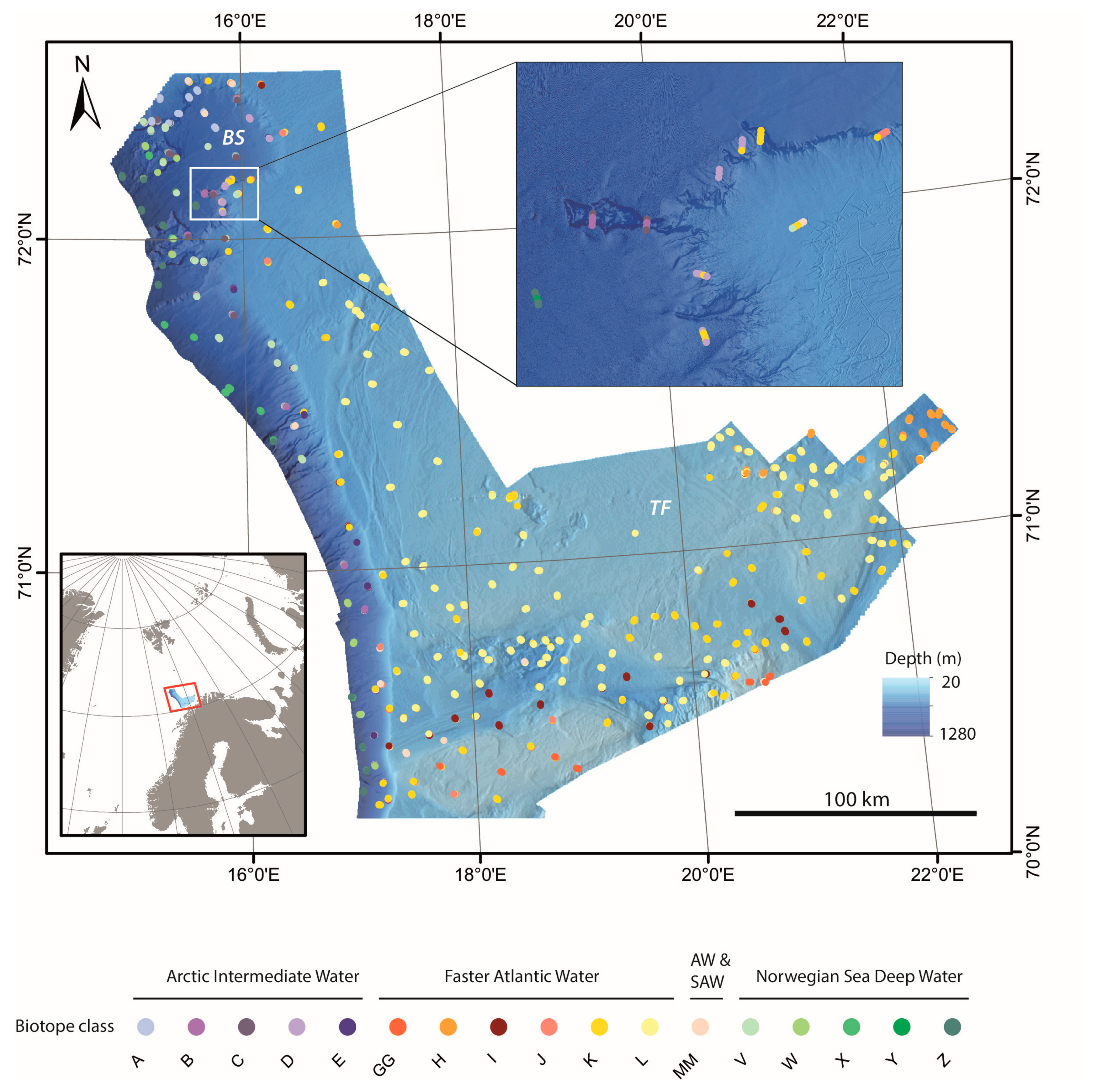
2.1. Study Area

The study area (Figure 1) includes part of the continental shelf and slope in the western Barents Sea, off Northern Norway. This location was selected due to the availability of multiple suites of oceanographic model data which we use here in a comparative case study for modelling the distribution of seabed biotopes. This is the only area within Norwegian waters where these alternative versions of oceanographic model simulation results are presently available, and where video data (necessary for the interpretation of seabed geology and biotope classification) have already been acquired by MAREANO. Previous studies explain the geological [42,43,44], oceanographic [45], and biological context of the region [11].

MAREANO video and sampling surveys were conducted in this area during several research cruises between 2006 and 2010, providing the necessary biological, geological, and geochemical data to supplement multibeam mapping (bathymetry and backscatter data) for the development of MAREANO’s portfolio of map products [46,47].

2.2. Biotope Modelling

Machine learning algorithms are now in widespread use for seabed HDMs and related studies. One of the most popular approaches, random forest (RF) modelling [48], is used in this study. Random forest, and variants of this approach, are generally well matched to seabed geospatial data and are a good fit for predicting the distribution of biotopes [11]. As RF and related modelling has been more widely utilised in spatial applications, the need for adaptations or extensions to standard methods has emerged including the need for spatial cross-validation [49,50,51,52] and methods for determining spatial validity [39,53,54]. Selected methods for addressing both these issues are adopted in the present study.

We produced HDMs of biotope distribution, associated accuracy statistics, spatial validity, and uncertainty using four biotope model setups, each employing a different suite of predictor variables. Three of our HDM setups include predictor variables from each of the available oceanographic model data (Section 2.2.2) while the fourth is a baseline model that does not use oceanographic data. The modelling workflow is described in Section 2.2.3. We first introduce the HDM response and predictor variables.

2.2.1. Response Variable–Classified Biotope Point Data

Video sample stations which were classified into biotopes in a related study for a wider area in the Norwegian part of the Barents Sea [11] serve as the response variable in our biotope HDMs. Full information on the video data, taxonomic identification and classification process, and biotope characteristics are detailed in Buhl-Mortensen et al. [11]. Briefly, the classification is based on species compositions identified from MAREANO video data using a TWINSPAN analysis. Each classified biotope observation (point shapefile of video sample locations) used in HDM represents a summary of the benthic megafaunal community observed on video over a distance along the seabed of approximately 200 m. The spatial distribution of these classified points is shown in Figure 1 with the inset map highlighting how each 200 m classified biotope sample originates from video lines which are c. 700–1000 m long. Usually there is only one video line at a video reference station, hence 3–4 samples, but occasionally additional video surveys lead to more samples at a reference station. Since the spatial extent of the present study is smaller than that covered by Buhl-Mortensen et al. [11], not all reported biotopes are present within the study area or are observed too sparsely to facilitate HDM. We have therefore modified the classification slightly, merging biotope classes with too few observations (<20) into a higher level in the classification hierarchy. Figure 1 shows the modified classification with the water masses associated with the biotope classification hierarchy indicated in the legend. This provides consistency with the previously published results, with necessary modification to facilitate this study. The fact that the classification may not be optimal for the study site is not a major concern since our aim is to explore the effects of the different oceanographic model data in HDMs rather than trying to make the most reliable biotope HDM for this area.

2.2.2. Predictor Variables–Oceanographic and Common Baseline Data

The predictor variables used in this study were selected to facilitate the comparative study presented here and are a subset of all variables considered in biotope modelling over the wider area reported by Buhl-Mortensen et al. [11]. Each variable type is described in turn below.

Bathymetric Data

Bathymetric data are from multibeam surveys conducted for MAREANO by the Norwegian Hydrographic Service (NHS). The surveys utilised multiple systems and survey vessels and are of varying resolution and quality. Bilinear resampling was used to convert the original high-resolution data (5–10 m) to a 200 m grid, matching the distance over which biotope observations are summarised. This resampling operation also minimises any quality differences between the original resolution data. Note that no bathymetric derived terrain attributes (slope, ruggedness, etc.), commonly used in seabed HDMs, have been included in this study. This is a deliberate omission based on (a) a desire to simplify the study and retain focus on the differences between the model predicted outputs based on the various suites of oceanographic variables, (b) the fact that terrain attributes have been shown to be of quite minor importance relative to oceanographic and geological variables in our previous biotope modelling work at the relevant spatial scales, including Buhl-Mortensen et al. [11]. This observation is based on variable rankings obtained from HDMs where all these variable types were included (c) methods for the derivation and selection of terrain attributes, including data resolution are a topic unto themselves which is beyond the scope of this study and would detract from the investigation of the influence of the oceanographic variables if included. We use only a minimum number of non-oceanographic variables (bathymetry, sediment class, X, Y) to construct a baseline model which acts as a yardstick against which we can compare the outputs using the different suites of oceanographic variables.

Geological Data

Sediment grain size information used in this study comes from the 1:100,000 classified polygon grain size map produced by the Geological Survey of Norway (NGU) for MAREANO (available from https://www.ngu.no/en/topic/datasets). Grain size classes are interpreted from acoustic, video, and physical sample data and represent dominant sediment types at the given map scale. Bellec et al. [55] provide a recent summary of the methods for sediment map production, based on earlier standards [56]. The categorical grain size data were converted to a 200 m raster grid for use in our HDMs.

A map of broad-scale geomorphology (MAREANO landscape map) was not used in the present study despite being a useful predictor variable (although ranked with lower variable importance than sediment class) in the Buhl-Mortensen et al. [11] study. This is because, within the limited study area, there are relatively few landscape classes present. In addition, we aim to minimise the number of common (non-oceanographic) variables used in the present study and therefore retain only the generally more important sediment class from available geological variables.

Geographic Variables

Raster grids of X and Y coordinates (UTM33N, WGS84) were used as additional variables in all models. These were generated using the init() function from the raster package [57] in the statistical software environment, R [58] using the 200 m bathymetry data as a template. We note several discussions in the literature regarding the wisdom of using geographic variables in spatial modelling. Whilst several authors argue for their inclusion, others note the limitations and potential issues related to their use (e.g., [59,60]) for HDMs of biotope distribution across large areas (hundreds of kilometres), we have found that these variables often serve as useful proxy variables for some controlling variable we do not have data for and generally improve model outputs. Inclusion of these variables supports the uncertainty methods we are exploring in this case study, although we remain mindful of the limitations of this type of variable for spatial modelling in general.

Oceanographic Model Data

We used three separate suites of oceanographic variables in our case study, each from oceanographic model applications produced independently by the Institute of Marine Research for different purposes. Below we provide a brief technical overview of the oceanographic models highlighting the differences between models which may help explain the variations in their outputs (Figure 2) and potential limitations for use in HDMs.

The coarsest data are extracted from the Nordic-4km (N4k) model [61,62] for the years 2005–2007 which are deemed to be reasonably representative. The N4k model was designed primarily to investigate hydrography and transports in the Barents Sea with focus on the flow of surface and Atlantic water. Although the model has provided realistic results for the surface and intermediary ocean levels, it is shown that the model has deficiencies in deep basin hydrography. However, we have not clarified if these offsets have any significant implications related to the circulation pattern. The coarse horizontal resolution also makes the model unsuitable for detailed analyses, but it is the only model (excluding global alternatives, generally of even poorer resolution/quality) presently available for large parts of Norwegian waters.

The Barents-800 (B) model is a standard, surface optimised, ROMS model, at 800 m resolution. It is an extension of the NorKyst-800 model [21] run for 2010 only. The Barents-800 model was selected for use here in preference to the longer historical run by the NorKyst-800 model (1995–2018 as explained in Asplin et al. [21]), which also covers the study area, because results from Barents-800 were used in the precursor to this study [11]. The unified results over a wider area, beyond the extent of the NorKyst-800 model, afforded by the Barents-800 model, were advantageous to that study. Note also that the Barents-800 model was forced by input from the N4k model along its open boundaries.

The Sandwave-800 model (SW), also at 800 m resolution and also forced by input from the N4k model along the open boundaries, is an inverted (bottom-optimised) model [45] which was produced for a project studying sandwaves on the continental slope [43,44]. The Sandwave-800 model is set up such that it has more layers near the seabed, and therefore can more accurately represent near-seabed conditions. The extent of the Sandwave-800 model was limited due to the specific objectives of the original project for which it was produced. Consequently, this model dictates the boundaries of the present study area. It is currently the only bottom-optimised model available for offshore areas of Norway.

Regardless of their original, coarser resolution (

Table 1. Summary of the variables considered in each biotope HDM-Base (no oceanography), N4k (oceanographic variables from Nordic-4km model), B (oceanographic variables from Barents-800 model), SW (oceanographic variables from Sandwave-800 model). All oceanographic variables are the modelled values from the deepest layer of the N4k, B, and SW models respectively (i.e., near-seabed values).

Variables		HDM
		Base	N4k	B	SW
Common variables	Bathymetry	5–10 m floating point geotiff (resampled to 200 m)
	Easting (X), Northing (Y)	200 m
	Sediment class	1:100,000 polygon (resampled to 200 m)
Oceanographic variables	Temperature (Maximum, Minimum, Mean *)	n/a	4 km Surface optimised floating point geotiff (resampled to 200 m)	800 m Surface optimised floating point geotiff (resampled to 200 m)	800 m Bottom optimised floating point geotiff (resampled to 200 m)
	Salinity (Maximum, Minimum, Mean)
	Current Speed (Maximum, Mean)

* Mean temperature was removed following VIF checks for multicollinearity and not used in our HDMs (see Section 2.2.3).

) all three suites of oceanographic variables were resampled to 200 m resolution using bilinear resampling. This resolution matches the distance over which biotope observations are summarised. In this study, we restrict ourselves to those variables which are available in all three model suites (Table 1). Maps of example variables from each of the three oceanographic models are shown in Figure 2 where we see that near-seabed conditions appear somewhat different in each model. For HDMs, it is important how these differences manifest themselves at the biotope sample locations (Figure 1). We performed some exploratory analysis to help visualise differences in the distribution of our response variable (biotope samples) across each of the oceanographic models. Some examples are shown in Appendix A.

2.2.3. Biotope Modelling Workflow

The HDM workflow is summarised in Figure 3 and the predictor variables available for each HDM setup are listed in Table 1. Response variable data was common to all HDM setups. Prior to the main modelling and prediction steps, some initial preliminary data exploration was undertaken to explore how the biotopes (response variable) are distributed in relation to the oceanographic predictor variables and to what extent they are distinct relative to these variables. Brief checks for multicollinearity were undertaken using variance inflation factor analysis (VIF), but only one variable was removed (mean temperature) due to being particularly correlated with other variables. This process should be taken much further along with testing for individual variable significance in most biotope modelling studies, but here it would be counterproductive when comparing the influence of variable suites from different oceanographic models, not individual predictors.

Biotope HDMs were developed for each suite of predictor variables (Table 1) in R using the Ranger implementation of random forests [63] via the Caret package [64]. RF modelling uses a machine learning algorithm that provides a convenient and suitable method for the present study, consistent with that used by the authors in [11]. Following initial testing to explore suitable model settings and based on our experience with modelling the wider area [11], the same settings were used to generate all HDMs. Since the RF approach will naturally result in slight differences between runs, fixed seeds were used to ensure that the results are fully reproducible. To facilitate examination of the relative importance of predictor variables, we computed unscaled permutation importance for each HDM by activating the appropriate settings in Ranger via Caret.

To provide a broader basis upon which to evaluate HDM results and associated spatial validity and uncertainty, we developed ensemble HDMs set up to use each of the four suites of predictor data variables (Table 1) following the approach described by Mitchell et al. [36] which also allows us to obtain their combined confidence measure (Section 2.2.5). The ensemble approach to HDM is one that is gaining popularity for many applications. Here, it allows us to both investigate the variation in results between HDM runs and to summarise results, including relative variable importance, over many models. To facilitate the development of our ensemble HDMs, the original sample data were split, with replacement, into 25 training- and test- sets with an 8:2 ratio using methods to preserve the ratios of the response variable (biotope class).

To facilitate model tuning (not used in [36]), and later assessment of the area of applicability (Section 2.2.4), our training data were further split into 10-folds which are used for cross-validation (CV). We use spatial CV as opposed to standard random CV, in keeping with the recognised need to use cross-validation methods adapted for spatial data (e.g., [49,50,51,52]). Spatial CV was implemented in the CAST package [65]. This approach is well suited for applying spatial CV for irregularly spaced data and/or spatially clustered data like our video samples (Figure 2) which contain several biotope samples at each reference station. As in our earlier study [11] we use CAST’s function CreateSpaceTimeFolds() to apply leave-location-out (LLO) CV. In LLO CV, HDMs are repeatedly trained by leaving the data from one location out and using the respective held back data for model validation. In our case, we define the video reference stations as the location and create 10 folds. Hence, ten model runs are performed, each leaving out one tenth of video reference stations and holding these data back for validation.

HDM performance using LLO spatial CV assesses models’ ability to predict to new locations, since the held-back data are used to test model performance distant in space from the training data. This gives more realistic performance estimates than those based on random CV [49] where the folds are not spatially aware. We used automatic model tuning facilities for Ranger in Caret which allow different options for several tuning parameters (mtry, splitrule, min.node.size) to be tested during cross-validation. The tuneLength argument was set so that all predictor variable combinations were used in the random tuning parameter search. The Kappa statistic was used as the assessment metric for model tuning. This is a reasonable, if not ideal metric, which remains in widespread use for multiclass problems [26]. The model option with the highest Kappa value (i.e., the best-tuned cross-validated HDM) was retained from each of the 25 runs and used further in analysis and prediction.

For each of our four HDM setups, using the different suites of predictor variables, the same 25 training and test sets were used to generate HDMs including classification and probability results (Figure 3). From these, we generate standard (non-spatial) accuracy statistics, including balanced accuracy [66], overall Kappa [67], and accuracy, as well as spatially explicit validity and confidence assessments as outlined below.

2.2.4. Area of Applicability

HDMs based on machine learning are good for modelling complex relationships but gaps in predictor space cause problems because the model has no knowledge of the expected outcome in these areas. To determine whether our model is valid in such locations or not, we need a measure for how well it can predict into unknown space i.e., combinations of environmental variables the model has never seen. One such method, developed by Meyer and Pebesma [39], is to use a dissimilarity index (DI) that incorporates the (RF) model’s weighting of each variable in quantifying how well the total environmental space is represented by the training data both in space and values. The DI in turn provides the basis for defining a model’s area of applicability (AOA) which summarises where the model can be considered valid. In a broad sense, the AOA is a component of model uncertainty but since it is based on quite different principles and gives an indication of overall spatial validity, rather than the potential confusion between classes, we keep it separate in this study. The AOA threshold is provisionally set as the outlier-removed DI of the (spatially) cross validated training data based on results from the simulation study reported by Meyer and Pebesma [39]. The AOA is implemented in the CAST package for R, [65] which since version 0.4.2 allows categorical predictors to be used. Here, we compute summary statistics for DI and AOA based on spatial CV for each of our 25 models for each suite of predictors. Whilst AOA is an emerging concept, the AOA and DI results should provide information which is complementary to the spatial uncertainty indices and therefore information which is useful in elucidating differences between the HDMs based on different suites of predictor variables. The extent of the realised AOA should also be important in prioritising which predictor variables, in particular which oceanographic model data, should be prioritised for future use in similar modelling work.

2.2.5. Spatial Uncertainty

Several authors have discussed and applied metrics for spatial uncertainty in classification studies. Drawing on their own work and that reported in the literature, Fiorentino et al. published an opinion paper [29] advocating increased use of soft classifications in spatial ecology. Citing several examples from seabed habitat mapping studies, the authors highlight use of the Burrough’s confusion index [27], Pielou’s evenness index [28], and a red-green-blue (RGB) representation of a multiband raster comprising the probability of the three most likely classes for each pixel. The latter is not strictly quantitative but each of these approaches gives insight into the spatially explicit uncertainty underlying the predicted classification. The combined confidence index introduced by Mitchell et al., [36]), comes from a similar school of thought. It aims to offer a more accessible alternative for quantifying spatially explicit uncertainty to approaches cited by the authors which frequently have unrealistic demands for the volume of test data, way beyond what is generally achievable in the marine realm. Computation of their combined confidence index is dependent on multiple model runs, making it more computationally intensive than the abovementioned indices which can equally well be applied to single HDM outputs. A selection of these quantitative methods were applied here in addition to visual comparison of the classified map.

Visual Comparison of Classified Map

The first and simplest of the methods used, is just a visual comparison of the classified maps produced using each of the four suites of predictor variables. Both the individual and ensemble model outputs from R were exported as geotiff files for easy display in ArcGIS 10.7.1 (ESRI) which provides a more convenient interface for map exploration than R. Predicted biotope distribution from individual model runs gives us a visual insight into the relative stability and agreement of the models from each suite of predictor variables between runs. The ensemble model displays the most commonly predicted class per pixel across all 25 model runs (i.e., the maximum frequency class as per the Mitchell et al. [36] code used). This can be considered as the final output, which is linked to the combined confidence measure below. To aid this visual assessment, we also compute the class variety for each pixel in our ensemble HDMs using ArcGIS Spatial Analyst. This statistic indicates the number of different biotope classes predicted for each pixel ranging from 1 (all ensemble HDMs agree) to 4 (different biotope predicted by each of the four HDMs).

Combined Confidence

Combined confidence (CombConf) is a metric proposed by Mitchell et al. [36] as a relatively simple, spatially explicit summary, allowing users to assess to what extent a map offers reliable (stable) results and where they can most trust the classification. The computation of CombConf is dependent on multiple model runs being performed (generally 25 or more) using bootstrapped training and test data. The CombConf metric merges model stability with the likelihood of the most common class occurring at any location on a pixel by pixel basis and is computed by multiplying the frequency of the most common class and the average probability of the most common class for each mapping unit. We expect CombConf to be low near class boundaries where there is a transition between the most likely class, but the effects of this should be moderated by the plurality vote for the most common class so class boundary effects should be less than, for example, those from the confusion index. We used the relevant part of the script published by Mitchell et al. [36] to generate the CombConf outputs but implemented a modified function to generate an ordered probability raster stack (identical to MaxClassAveProb in Mitchell et al.’s script [36]) which could more intuitively be reused in other metrics below. For each pixel, we obtain a stack of the probability values across all 17 biotope classes ranked from highest to lowest. The result is identical to the values produced as input to the average probability computation using the Mitchell et al. [36] method but offers a more convenient workflow for use in the present study.

Confusion Index

The confusion index, introduced by Burrough et al. [27], originated from soil sciences but has seen several applications to seabed mapping studies (e.g., [68,69]). We use the simpler alternate formula from Burrough et al. [27]:

$$CI=\frac{p_{max-1}}{p_{max}},$$

(1)

where p_max is the highest probability for any location (pixel) and p_max−1 is the second highest probability for the same pixel. In the present case study, the probabilities used in Equation (1) are the average probabilities for the most common class in our ensemble models. For single (non-ensemble) models, the highest probability and second highest probability for each location (pixel) would be used directly.

CI provides a measure of how dominant the most likely class is relative to the second most likely class on a scale of 0 to 1. Where CI approaches zero, then the most likely class dominates i.e., there is little confusion, but high CI values approaching one indicate confusion, with the second most likely class having a similar probability of occurrence to the most likely class. We expect CI to be high in transition zones between classes but a high CI across wider areas of the map indicates poor separation in the probability of occurrence i.e., high levels of class uncertainty.

We also exported multiband rasters of the top three average probabilities from our ordered probability stack. These can be displayed as RGB images with colour bands corresponding to each of the probability layers. The results give an initial insight into uncertainty [68].

Shannon Entropy Index

Similar to the Pielou evenness index [28] mentioned by Fiorentino et al. [29], the Shannon entropy index has been used by several authors as an uncertainty measure for soil classification maps (e.g., [32,70]), so was favoured in this study. Shannon entropy [30] is a generic method (from which Pielou Evenness is computed) which has recently been adopted for uncertainty quantification in several spatial classification studies broadly similar to our biotope HDMs (e.g., [32]). It quantifies the overall uncertainty associated to the probability of encountering each class. The scaled Shannon entropy index (H_s) [70] is given by:

$$H_s\left(x\right)=-{\displaystyle \sum }_{n=1}^N{p}_n\left(x\right).{\log }_N\left(p_n\left(x\right)\right),$$

(2)

where p_n(x) is the per class (n) probability map and N is the total number of classes, used as the base of the logarithm. Alternate versions of H_s can be computed using other bases (commonly log₂ or log_e), but the scaled version (Equation (2)) outputs values scaled between 0 and 1 which may be useful for combination with other outputs.

In the present case study, the probabilities used in Equation (2) are the average probabilities for each class in our ensemble models. For single (non-ensemble) models, the class probabilities would be used directly. At locations where the probability of one class equals one and the others are zero, then H_s = 0 (no uncertainty), whereas where all classes have equal probability H_s = 1 (maximum uncertainty). Note that this index offers only an internal uncertainty measure, it is not checking how correct the classification is, merely how well the class probabilities are separated.

In order to summarise the results of our uncertainty analyses, we also created density plots for each HDM for each uncertainty metric. Both overview plots for the entire area and plots per class were created. The class plots were produced by masking each uncertainty map (CombConf, CI, and entropy) by the areas covered by each biotope in the respective ensemble maps for each model suite.

3. Results

3.1. Accuracy Statistics

25 HDMs and one ensemble HDM were successfully produced with associated classification and probability results for each of our four suites of predictor variables (Base, SW, B, N4k—Table 1). Using the (as yet unused) bootstrapped test data, we computed the accuracy statistics summarised in Figure 4.

These non-spatial accuracy statistics indicate that there is negligible difference in the overall accuracy between the four ensemble models. We do observe some differences in terms of which classes are most accurate, but these are relatively minor, with the same classes generally showing accuracy issues. For example, classes C, E, J, MM, and Y show a consistently wide range (low average) of balanced accuracy scores across all HDMs, we suspect this is primarily linked to the relatively low number of samples for these biotopes. Additional accuracy and Kappa statistics from constituent model’s 10-fold spatial CV also do little to differentiate between the models. These values are, as expected, somewhat lower values than the results from comparison with the test data which were subdivided on class rather than spatial variables. Although supposedly offering a more realistic assessment of the models’ ability to predict to new locations [49], the overall accuracy and Kappa statistics from spatial CV seem to be just as ineffective at distinguishing between our HDMs as those based on comparison with test data.

3.2. Relative Variable Importance

The relative importance of each predictor variable varies across each of our four HDMs. In addition, the importance varies across the constituent models for each ensemble. This information is summarised in the boxplots in Figure 5. Across all HDM, bathymetry is the most important variable (barring outliers in the N4k model). In the base HDM, this is followed by the geographic variables X, Y with sediment class contributing minimally. In the other HDMs, sediment class is often more important than bottom current speed, possibly because the two are related, with coarser sediments occurring in areas with higher current speeds. Geographic variables are of moderate importance in all HDMs containing oceanographic variables, suggesting they are still a proxy for some indirect effect not captured in the other variables. In both the N4k and SW HDMs, temperature variables are next most important to bathymetry. Temperature variables are also important in the B HDM, but here they are of similar importance to mean and maximum salinity. These results, with salinity relatively more important in the B model, highlight how we can gain a different impression of what we interpret biologically, depending on the predictor variables available. In reality, the water masses are not different but the representation of them across the three oceanographic models is (Figure 2), especially near the shelf edge where it is challenging to represent that water masses of different densities are forced up and down the slope due to the diurnal topographic waves [45].

3.3. Visual Comparison of Classified Biotope Maps

Examining the spatial distribution of biotopes output by the ensemble models (Figure 6), we see that there is remarkably little difference in the general distribution of biotopes, with at least the most dominant biotopes exhibiting similar patterns of distribution. When we compare these results visually with the biotope sample data (Figure 1), it appears that the ensemble method has produced reasonable results across all HDMs, at least when viewed at a broad scale, regardless of the predictor variables used. These initial observations would also seem to confirm the similarities in our accuracy statistics (Figure 4).

Even the baseline model (Figure 6a) with no oceanography data included appears to give a decent indication of the biotope distribution and there are only relatively fine scale differences in biotope distribution and/or the extent of individual biotope classes across all HDMs, as highlighted by the class variety map (Figure 7). Based on these ensemble results alone, it appears that, for broad-scale predictions of biotope distribution within this case study area, there is no major impact of including oceanography data in any form. Nevertheless, we reserve judgement on which, if any, oceanographic inputs are best suited until we have seen the results of the spatial validity and uncertainty analyses.

Examination of the output from individual spatially cross-validated HDMs that are input to the ensemble result, however, provides further insight into the model stability and reveals important differences between the stability and quality of the output across each of our four ensemble HDMs (see Supplementary Material S1). Whilst the ensemble results give the same general impression, the predicted biotope distribution maps from the 25 runs of each HDM-setup show that the results of the constituent models are far from consistent. This leads us to question the reliability of the ensemble map, or at least desire more information on its associated validity and uncertainty.

Since non-spatial accuracy statistics (Figure 4) appear to do little to discriminate between spatially differing model predictions, we see that it is important to include a spatial check on model outputs, at least visually but preferably, using quantitative methods.

3.4. Spatial Validity

A summarised version of the AOA results is shown in Figure 8. We observe differences in the AOA across each of our HDMs. The SW HDM has the least area outside of the AOA (gaps in weighted predictor space), followed by the B HDM, whilst both the N4k and Base HDMs show quite large areas falling outside of the AOA, suggesting weaknesses in these models. Of the two latter HDMs, the N4k model result reveals the broadest and most consistent areas with problematic AOA. This is likely because more variables are included in the N4K relative to the Base model, leading to more scope for variation between model runs.

3.5. Spatial Uncertainty

The results shown in Figure 9 illustrate the results of the CombConf index which assesses the stability of prediction across the 25 constituent models. It is immediately clear that CombConf maps do indeed summarise the instabilities which are visible when examining the 25 constituent models, but which are not clear in the ensemble maps themselves. Firstly, we can observe that the uncertainty varies across the study area. This is new information that the non-spatial accuracy statistics did not capture. Further, as we compare the results from all four HDMs, we note that the uncertainty is consistent in some areas but exhibits distinct differences in others. We observe low confidence in all four models on the continental slope. This uncertainty extends beyond class boundaries, suggesting that this is an area that is difficult to predict using the available training data, probably compounded by the relatively high number of classes observed in this area. This result is not unexpected when we refer to our preliminary data explorations (Appendix A) where we saw that the slope-associated classes (A-E) are quite poorly separated with respect to several oceanographic variables. In addition, we have relatively few samples for each of these classes. Elsewhere across the maps we see that the uncertainty varies away from class boundaries for some of our HDMs, which, in this case, is directly indicative of instability and low confidence.

CombConf results from the Base model on the shelf shows linear artefacts in uncertainty, reflecting the issue with overreliance on geographic variables mentioned above. Some parts of the map are quite certain, but it is very certain in far fewer areas than the other HDMs. The N4k model has large areas of certainty on the shelf but the weaknesses in this model output are suggested by the relatively high uncertainty across much of Tromsøflaket (see Figure 1 for location) even relative to the Base model. This may imply that the oceanographic variables from the N4k do not aid the classification over and above the information already included in the Base model. Instead, the extra variables, which do not adequately capture the variations in water mass properties relevant to biotope distribution, may lead to more uncertainty. This may also be linked to the fact that Tromsøflaket has a low sample density due to logistical issues during fieldwork. Both the B and SW models perform better, but whilst the B model still indicates uncertainty in parts of Tromsøflaket and on the shelf to the northwest, the SW model displays uncertainty that is almost entirely linked to class boundaries (i.e., where it is of least concern), in contrast to the N4k model (Figure 10).

The SW model appears, however, less certain than the other models on the shelf directly above the Bjørnøya slide (see Figure 1 for location). This is likely due to lower average probabilities for the most common class relative to other classes in the SW model. Whilst the most frequent class is still dominant (has a relatively low CI), the average probability values for the SW model are slightly lower than for the other models. At the same time, the probabilities for the next two most frequent classes are slightly higher than for the other models. A first impression of this difference in the probability weighting between models is visible in RGB images which combine the average probability values for the top three most common classes (Appendix B). These RGB images, whilst largely qualitative, can give a useful first indication of uncertainty issues.

The CI results from each of our four ensemble models are shown in Figure 11. The confusion index (CI) provides a useful summary of where the class separation is most problematic. As expected, high CI values do occur close to class boundaries, but other high CI values beyond these zones are indicative of questionable model performance (e.g., on Tromsøflaket). Although based on different criteria, these maps present quite a similar story to that gained from the CombConf results. All models show high confusion on the slope as they did with the CombConf index. Since the CI is not scaled by probability, however, the confusion is potentially overexaggerated in areas where the probabilities are relatively high (on the shelf), making them appear similar to areas where the probabilities are lower (on the slope).

Figure 12 again shows clearly that the continental slope is the most uncertain part of the predicted maps, across all model suites. Entropy results for the B and SW models are broadly similar, showing reasonable separation in class probability across much of the shelf area. The N4k model also shows reasonably good results and is not as affected by problems on Tromsøflaket as the other indices were. The Base model only achieves the lowest category of entropy in a few locations with most of the shelf having more similar class probabilities (high entropy).

Based on our results, the Shannon entropy maps appear to provide useful supporting information showing more generalised trends in confidence that are not overly influenced by class boundaries. This can be very useful supporting information for the classified maps.

Density plots for each of the uncertainty indices can complement the maps presented above (Figure 9, Figure 11, and Figure 12). Overview plots showing the relative distribution of uncertainty values across each of our four ensemble HDMs as well as density plots by class are presented in Appendix C. The latter are particularly useful in assessing which classes are worst affected by spatial uncertainty issues, although the plots themselves are non-spatial.

4. Discussion

This study aimed to discern whether data from any of three oceanographic models, with different properties, was better suited to use as predictor variables in seabed biotope HDMs. We used an ensemble modelling approach and accompanying metrics of spatial validity and uncertainty to compare the performance of HDMs using four suites of predictor data, three of which included different versions of oceanographic data, the fourth using only basic predictor variables common to all models. The results illustrate the benefits of generating validity and uncertainty metrics to accompany classified biotope maps and indicate that different recommendations could be drawn based on the scale at which the maps are considered relevant. Here, we draw some initial conclusions at broad and finer scales, evaluate the metrics of spatial validity and uncertainty, make a provisional assessment of which oceanographic predictor suite seems most preferable going forwards, and discuss the limitations of this work.

4.1. Scales of Evaluation of the Classified Maps

Classified biotope maps were produced that are broadly similar for ensemble HDMs based on each of the four suites of predictor data, but clear differences are visible when zooming in to finer scales.

All four ensemble maps could potentially be used at scales of around 1:2 million (whole area) where they may be suitable for regional applications focussed on the most widely occurring biotopes. The maps could also possibly be used to guide future efforts for finer resolution mapping or modelling within the dominant classes. At this scale, and with these purposes in mind, it does not seem important what type of oceanographic predictors are used, or, cautiously, if they need to be included at all (given that the Base model, without oceanographic predictors performed similarly, and for some areas, like Tromsøflaket, better than those using the coarsest version of oceanography data).

However, when zoomed in to finer scales, including the still relatively coarse 1:400,000 scale at which our 200 m biotope map would be suitable for conversion to a polygon map according to Tobler’s rule [71], differences are observed across ensemble maps based on the different suites of predictors. Scales of 1:400,000 and finer scales might be relevant for marine managers searching for the best locations to set boundaries for management areas or when using models to guide targeted sampling. Given the differences at these finer scales, it is difficult to know which map to trust the most without supporting (e.g., uncertainty) information. Yet the observations of linear artefacts in several of the constituent baseline HDMs do suggest that oceanographic predictors are useful in refining these finer scale predictions.

The ensemble models conceal much of the variation between model runs, indeed this is the very point of ensemble models-many outputs, even including single divergent (‘bad’) ones leads to a better overall result, provided the ensemble is based on enough results. Here, we followed Mitchell et al. [36] and used the standard practice of 25 bootstrapped models [72]. Initial testing with just ten bootstrapped models produced much less satisfactory ensemble models. Intuitively it makes sense to use more models: with fewer models, stability is not reached unless their results are similar. Yet, more models require more investment in terms of processing resources and may become prohibitive when modelling over large areas with large volumes of input data.

It is possible that constituent HDMs trained on the full dataset (without withholding some data for testing) would have higher stability between runs. There is, however, no guarantee that the results would approach the best of those from the 25 bootstrapped models developed here. Given the relatively uniform results from each of our models, it seems that ensemble modelling is a smart approach to reduce uncertainty and to provide a more extensive basis for production of accompanying spatial uncertainty maps. The (non-spatial) accuracy statistics do not provide an adequate means by which to distinguish between ensemble HDM outputs in the present study and risk, giving an overoptimistic summary of performance. We therefore recommend that reported uncertainty should be spatially explicit and preferably incorporate probability information which facilitates the use of metrics like those employed in this study. Where such computations are prohibitive, a basic measure of spatial uncertainty can be obtained simply from tallying differences in the classified map outputs from bootstrapped HDMs e.g., calculating the pixelwise standard deviation [7] or the frequency of occurrence component of the CombConf index to summarise how the map varies between runs.

4.2. Spatial Validity and Uncertainty Indices

The area of applicability [39] appears to offer a promising method for checking the spatial validity of HDMs which incorporates variable weighting. Weaknesses in our AOA results were identified in all our HDMs regardless of the input predictor variables, although the results using 800 m model data (SW HDM, followed by B HDM) showed the least AOA-related problems. We suspect that the AOA may be underestimated in this study due to the inclusion of categorical predictor variables (sediment grain size classes) which are mapped at 1:100,000. Unlike the other continuous predictors, the HDM and hence the AOA analysis has no way of knowing which sediment classes are most closely related, which may lead to more areas than strictly necessary being masked out as outside the AOA. Further investigation on the best way to incorporate such categorical variables is advised, along with possible refinement of the AOA threshold. Possible solutions include using ordered variables, or conversion of the sediment grain size classes to generalised sediment fractions [73]. We also note that the survey design (video stations) was made long before these oceanographic datasets were available. More recent standard MAREANO practice is to use the best available oceanographic model data in station planning using methods suited for achieving good coverage of environmental space, e.g., [74]. For the purposes of this study, the AOA provided a useful basis for HDM comparison, with several areas being highlighted to have AOA issues, particularly in the Base and N4k models. Further, the case study provides a means to raise awareness of this spatial validity topic both to marine scientists and resource managers.

All uncertainty metrics concur that HDM results on the continental slope are uncertain, regardless of the predictor variables used. This can be attributed to the high degree of environmental variation combined with quite a high number of biotope classes with relatively few observations in each class and little separation between classes in terms of several predictor variables. The study area, for which video surveys were planned prior to the availability of oceanographic data or development of MAREANO’s environmental variability index [75] which is used to guide sampling effort, currently has few samples relative to its environmental and biological complexity, particularly on the slope. Where possible, the sampling effort should be increased in such areas, although we recognise this is rarely likely to occur in costly offshore surveys. In the absence of additional samples, future biotope HDMs that include this area should consider the merging of these classes to increase the certainty. However, if the biotopes have very different biological characteristics, it may be preferable to retain the classes, even if this means accepting higher uncertainty. In any case, it is important that uncertainty information is flagged for map users so that they know which areas of the map can be trusted and which should be treated with caution.

All the uncertainty metrics used in this study provide important insights into the variations between our HDMs, thereby giving an insight into which suite(s) of oceanographic data may be preferable. Each metric offers a slightly different perspective making it difficult to select one best method.

Model stability is best captured by the CombConf measure since this is directly linked to the frequency of occurrence of the most likely class. This measure is made more useful by its intrinsic link with probability which means that class boundaries in areas with lower probabilities are highlighted as being more uncertain. This index provides a good overall measure of where the predicted most likely class is certain or potentially confused, yet it is dependent on a relatively large number of model runs so is probably better suited to final modelling (i.e., once final classes are decided upon) than initial model development (where classes may be considered for merging until an acceptable level of uncertainty is reached).

Maps of CI provide useful information but are dominated by (expected) high confusion near class boundaries. High confusion beyond class boundaries is of greater interest when identifying weaknesses in model predictions. For example, this index captures weaknesses in the N4k-based models in an area with few observations. The index is limited since it only considers confusion between the two most likely classes, when in fact three or more classes may have similar probabilities, as we see from the entropy results. It may be of value to combine this index with the entropy results.

The Shannon entropy maps provide a good general overview of where the maps are uncertain and this index is not fragmented by confusion (similar probabilities) at class boundaries in the same way as CI, or CombConf. This is an advantage on an overview level e.g., identifying areas which should be considered for merging or further sampling, however the lack of specific information on uncertainty at class boundaries means that the use of this index alone may be insufficient.

4.3. Based on the Map Results Which Oceanographic Data Do We Need, If Any?

Despite the superficial similarity between classified biotope model outputs based on the four sets of input data, at a coarse scale, the finer scale uncertainty and spatial validity results concur that, in this case, spatial uncertainty is minimised, and spatial validity maximised by using the SW data. This predictor suite still perpetuates some confusion on the continental slope that is common to all models, but otherwise appears to be the most stable and certain of the three being tested in this region. The SW data represent the only predictor suite that was bottom optimised.

The B model would be second choice: it retains some issues in relation to some uncertainty metrics, but seems to be fit for purpose at least for maps to be used at moderate scales e.g., 1:400,000, which is in keeping with the 200 m modelling resolution. Both the B and SW predictor suites are based on relatively fine scale (800 m) regional oceanographic models.

Whilst the ensemble classified maps based on the N4k and Base predictors appear superficially reasonable the uncertainty and spatial validity analyses reveal considerable problems with these HDMs. The N4k model shows large areas of uncertainty particularly in areas where few samples are available, but we suspect that additional uncertainty may be linked to the overly generalised nature of the oceanographic variables. The N4k oceanographic model that supplied these data was designed to cover a larger area (than the SW and B models) and therefore had a much coarser resolution (4 km). This may be too coarse to capture the biologically relevant oceanographic dynamics of the region of interest.

The Base model, while sometimes exhibiting lower uncertainty than the N4k model, is overly dominated by linear artefacts related to the geographic variables. These artefacts, which are also visible in some of the individual classified maps but are highlighted in most of the uncertainty metrics, are not acceptable. They indicate an over-reliance on spatial variables which have made the RF modelling akin to a spatial interpolation exercise from the training points (see variable importance plots Figure 5). Where X and Y variables are not sufficiently supported (diluted) by other variables, they are known to cause problems (e.g., [59]). We would not recommend using this model for fine (meso) scale applications.

Based on the results of this case study, we recommend incorporating oceanographic data in future biotope HDMs in MAREANO and similar studies. This data should be from oceanographic models of at least ~1 km resolution if possible, and preferably from bottom optimised models. High uncertainty associated with HDMs with no oceanography data or coarse oceanography data (4 km) mean that these variable suites are not advised for modelling at the finer scales relevant to MAREANO users (primarily marine managers and industry) unless spatial uncertainty and validity can be shown to be at an acceptable level. Although it is possible that the inclusion of additional, alternative predictor variables e.g., terrain attributes, could improve the B and N4k HDMs, the strong oceanographic characteristics of many biotopes [11] and the uncertainty/validity issues demonstrated here make it unlikely that the inclusion of such data could outperform HDMs including good (800 m) oceanographic data. This comparison has not been tested here but we recommend that if coarse oceanographic data are the only option, these may be included initially, subject to a full variable selection process, possibly including automated methods such as recursive feature elimination [76] or forward feature selection [49,59].

4.4. Limitations and Further Work

Random forest modelling provided a suitable method for the present study. We recognise that other modelling approaches could also be employed, but this study is focused on comparing results based on different suites of predictor variables, and their associated spatial uncertainty/validity, rather than on comparing different modelling algorithms as some other authors have done (e.g., Pearman et al., 2020).

The response variable used in this study (biotope classes [11]) was trusted as-is. MAREANO biotope classification is data driven and is updated as new video data are acquired and mapping is extended into new areas. Consequently, there is inherent uncertainty in the definitions of these classes. Indeed, in this case, the classes were defined from a much larger region than is covered by this study. This means that some biotopes were underrepresented and were merged to reduce class imbalance. Had they been analysed separately, they may have been grouped differently.

This imperfect classification system represents both a potential limitation and an opportunity in relation to the present study. Our results indicate that it would be beneficial to incorporate the outputs of preliminary HDM development, including spatial uncertainty metrics, into the process of refining the biotope classification itself. This is especially true where the classes themselves are being defined by local analysis, similar to the considerations discussed by Gonzalez-Mirelis et al. [77]. Classes associated with higher confusion or predictive uncertainty could then be examined further to double check whether a) there is an ecological basis for this confusion e.g., there are enough shared species and environmental conditions for a class to be better redefined as a subclass, or b) the model predictors are likely to be limiting that classes predictability e.g., the predictor suite does not adequately capture the different environmental conditions that drive a class divide. Either way, such classes may be candidates for merging for the purposes of modelling. In other cases, where the habitat classification is pre-determined e.g., using accepted systems such as EUNIS [78], NiN [79], CMECS [80], it may still be appropriate to use the uncertainty results to merge classes for modelling purposes. In both cases, this should ideally be done in consultation with major end-users to achieve a good balance in terms of information and acceptable levels of uncertainty.

The bottom-optimised Sandwave-800 model is only available for a small area which has constrained the geographical extent of this study. Consequently, we can only speculate as to the effects of using such data in wider area biotope modelling and any advantages they may have over the standard, surface-optimised Barents-800 model and related NorKyst-800 and Svalbard-800 models ([21] and [81], respectively). Unfortunately, finer resolution (both horizontally and vertically) models will generally cover smaller areas, due to computational restrictions, so in practice, resolution trade-offs may be required dependent upon the domain size of the HDM. Further, whilst our results have highlighted limitations with the coarser N4k model, we have not been able to explore whether a bottom-optimised model at this resolution would be a useful option.

Summary variables and limited (different) time periods for each suite of oceanography data are also a consideration. We may assume that spatial and temporal variability in near-seabed oceanography based on model results are an important environmental element linked to biotope distribution, but further research is required to ascertain at which scale(s) conditions vary in the real world. Since currents at depth are mainly driven by broad-scale density gradients which are hard to differentiate between interannually, this variable is unlikely to be much affected by the time period. Similarly, salinity does not have a recognisable interannual variation, but temperature gradients do. Nevertheless, it is likely that the main temperature gradients are represented realistically enough in each model period used here. In our HDMs we used only max, min, and mean values, not standard deviations, 90th percentiles etc. (as used in [11]), since these data were not readily available for all models. We recognise that temperature ranges and interaction variables may also be useful predictors. We also note a degree of uncertainty linked to the non-temporal MAREANO video surveys completed over the course of several years (and in different, non-winter months) whilst using oceanographic data only from non-corresponding available years across all seasons. Interannual and seasonal changes at depth have not yet been studied in any detail for the study area. Prioritising such work would help determine how relevant this may be in relation to habitat mapping and thereby how to deliver the most ‘representative’ results matched to the time periods over which MAREANO fieldwork has been conducted. Temporal considerations in relation to oceanographic data in HDMs are integral to the study by Young et al. [2] and their uncertainty estimates, whilst presented spatially, are related to time. To facilitate such studies in Norwegian waters, as well as exploring issues related to community connectivity, a breakdown of oceanographic model output into finer time intervals, including seasons per variable may be required. The variables may also have different explanatory power in relation to habitat distribution at different spatial scales. Oceanographic models capturing variations at sub-kilometre scales will be key in providing such information. Use of such data in biotope models is nevertheless likely to require resampling to finer resolutions more closely matched to the scale of seabed observations and it is important that such rescaling be done in an optimal manner which respects the limitations of the original model. We note that both Young et al. [2] and Pearman et al. [1] used alternative methods for rescaling the oceanographic data. We used simple bilinear resampling here, in keeping with the Buhl-Mortensen et al. [11] study, but improved methods may be considered for future work.

The workflow adopted here involves both validation and testing. This facilitated both model tuning (i.e., validity assessments based on spatial CV) and non-spatial accuracy assessments using bootstrapped test sets. This workflow could be considered overkill, particularly since we know in retrospect that the accuracy assessments did little to discriminate between HDMs based on different predictor suites. However, the multiple sets of training data from the train/test splits were well matched to the production of ensemble HDMs and associated uncertainty metrics. We therefore recognise some benefits in retaining both validation and testing components in future work where computing resources permit, but alternative workflows may also be suitable as long as they facilitate the production of both spatial validity and uncertainty metrics. The incorporation of spatial CV should be a priority for future studies. Besides facilitating more realistic performance metrics than random CV, it is also well matched with the computation of spatial validity metrics such as AOA. However, given the limitations of available tuning metrics such as the Kappa statistic [26], it may not be so important to tie the spatial CV to model tuning as we did here. Where ensemble modelling is used, then model tuning may be omitted in favour of a plurality vote from multiple models (e.g., [36]). If internal accuracy assessments from the spatial CV are considered sufficient for the study in question, then it may not be necessary to use test/training sets and produce bootstrapped HDMs with associated spatial uncertainty metrics for the ensembles. Rather, constituent models could be obtained from the spatial CV runs and used to generate classified predictions and class probabilities. A further advantage of this approach may be that the spatial uncertainty metrics and the ensemble classified map become linked to spatial CV, rather than being based on a random test/training class-based split as used in the bootstrapped models here. Further work is required to compare the relative merits of different approaches.

5. Conclusions

This case study produced four ensemble biotope HDMs using RF modelling to assess what types of oceanographic models are suitable for HDM. We examined the predicted classified output together with spatially explicit uncertainty and validity indices which helped compare the results. The HDMs differ only in the predictor variables included: one was built only with the baseline variables included in all HDMs, while the other three also included alternative sources of modelled oceanography data of varying resolution and parameterisation.

The spatial validity and uncertainty results gave unique insight into the differences between our four models and thereby an indication of which suite(s) of modelled oceanographic data are most suited to HDM at the scales considered here (meso-mega scale).

The main conclusions are as follows:

Classified biotope distribution maps can be produced from all our suites of predictor data based on available training data using ensemble RF modelling. There are negligible differences between the maps at broad scales such that any of these predictor sets could be used at scales of around 1:2 million (whole area) if the user is unconcerned with finer scale spatial uncertainty.

At a finer scale (e.g., 1:400,000), non-spatial accuracy statistics did not adequately summarise the differences observed between HDM outputs. Spatially explicit uncertainty analyses, however, revealed considerable differences between the HDMs and confirmed that some areas and classes are particularly difficult to predict. Each of the uncertainty measures used here (combined confidence, confusion index, Shannon entropy) provide complementary information, although there is some agreement between which areas of the map are most uncertain (continental slope, class boundaries) based on the different metrics. No single index used here captures all issues, therefore the use of multiple uncertainty metrics is recommended to support HDMs. Possible combinations of indices should be explored in future work.

The area of applicability appears to offer a promising method for checking the spatial validity of HDMs. For the purposes of this study, the AOA provided a useful basis for HDM comparison and the case study provides a means to raise awareness of this topic both to marine scientists and resource managers.

Based on these results, we cannot recommend further biotope model development at the mega-meso scale (i.e., matched to MAREANO mapping) using coarse (4 km or coarser) or no oceanography data unless the spatial uncertainty and validity of the predicted map can be shown to be at an acceptable level for end users. Oceanographic data from models of at least ~1 km resolution should be used if possible. These should preferably be bottom-optimised models, i.e., have a proper vertical resolution near the sea floor, which minimises uncertainty and maximises the spatial validity of classified biotope maps. Where ~ 1 km or better oceanographic model data do not yet exist in contiguous form, development of such oceanographic models should be prioritised for use in HDM.

References

- Pearman, T.R.R.; Robert, K.; Callaway, A.; Hall, R.; Lo Iacono, C.; Huvenne, V.A.I. Improving the predictive capability of benthic species distribution models by incorporating oceanographic data–Towards holistic ecological modelling of a submarine canyon. Prog. Oceanogr. 2020, 184, 102338. [Google Scholar] [CrossRef]
- Young, M.A.; Treml, E.A.; Beher, J.; Fredle, M.; Gorfine, H.; Miller, A.D.; Swearer, S.E.; Ierodiaconou, D. Using species distribution models to assess the long-term impacts of changing oceanographic conditions on abalone density in south east Australia. Ecography 2020, 43, 1052–1064. [Google Scholar] [CrossRef]
- Wilson, M.F.J. Deep Sea Habitat Mapping Using a Remotely Operated Vehicle: Mapping and Modelling Seabed Terrain and Benthic Habitat at Multiple Scales in the Porcupine Seabight, SW Ireland; Department of Earth and Ocean Sciences, National University of Ireland: Galway, Ireland, 2006. [Google Scholar]
- Guinan, J.; Brown, C.; Dolan, M.F.J.; Grehan, A.J. Ecological niche modelling of the distribution of cold-water coral habitat using underwater remote sensing data. Ecol. Inform. 2009, 4, 83–92. [Google Scholar] [CrossRef]
- Rubec, P.J.; Lewis, J.; Reed, D.; Santi, C.; Weisberg, R.H.; Zheng, L.Y.; Jenkins, C.; Ashbaugh, C.F.; Lashley, C.; Versaggi, S. Linking Oceanographic Modeling and Benthic Mapping with Habitat Suitability Models for Pink Shrimp on the West Florida Shelf. Mar. Coast. Fish. 2016, 8, 160–176. [Google Scholar] [CrossRef] [Green Version]
- Jalali, A.; Young, M.; Huang, Z.; Gorfine, H.; Ierodiaconou, D. Modelling current and future abundances of benthic invertebrates using bathymetric LiDAR and oceanographic variables. Fish. Oceanogr. 2018, 27, 587–601. [Google Scholar] [CrossRef]
- Ross, R.E.; Howell, K.L. Use of predictive habitat modelling to assess the distribution and extent of the current protection of ’listed’ deep-sea habitats. Divers. Distrib. 2013, 19, 433–445. [Google Scholar] [CrossRef] [Green Version]
- Buhl-Mortensen, P.; Dolan, M.; Buhl-Mortensen, L. Prediction of benthic biotopes on a Norwegian offshore bank using a combination of multivariate analysis and GIS classification. ICES J. Mar. Sci. 2009, 66, 2026–2032. [Google Scholar] [CrossRef]
- Dolan, M.F.J.; Buhl-Mortensen, P.; Thorsnes, T.; Buhl-Mortensen, L.; Bellec, V.K.; Bøe, R. Developing seabed nature-type maps offshore Norway: Initial results from the MAREANO programme. Nor. J. Geol. 2009, 89, 17–28. [Google Scholar]
- Elvenes, S.; Dolan, M.F.J.; Buhl-Mortensen, P.; Bellec, V.K. An evaluation of compiled single-beam bathymetry data as a basis for regional sediment and biotope mapping. ICES J. Mar. Sci. 2014, 71, 867–881. [Google Scholar] [CrossRef] [Green Version]
- Buhl-Mortensen, P.; Dolan, M.F.J.; Ross, R.E.; Gonzalez-Mirelis, G.; Buhl-Mortensen, L.; Bjarnadóttir, L.R.; Albretsen, J. Classification and Mapping of Benthic Biotopes in Arctic and Sub-Arctic Norwegian Waters. Front. Mar. Sci. 2020, 7, 271. [Google Scholar] [CrossRef]
- Gonzalez-Mirelis, G.; Buhl-Mortensen, P. Modelling benthic habitats and biotopes off the coast of Norway to support spatial management. Ecol. Inform. 2015, 30, 284–292. [Google Scholar] [CrossRef] [Green Version]
- Gonzalez-Mirelis, G.; Ross, R.; Albretsen, J.; Buhl-Mortensen, P. Modelling the distribution of habitat-forming, deep-sea sponges in the Barents Sea: The value of data. Front. Mar. Sci. 2021, 7, 496688. [Google Scholar] [CrossRef]
- Haidvogel, D.B.; Arango, H.; Budgell, W.P.; Cornuelle, B.D.; Curchitser, E.; Di Lorenzo, E.; Fennel, K.; Geyer, W.R.; Hermann, A.J.; Lanerolle, L.; et al. Ocean forecasting in terrain-following coordinates: Formulation and skill assessment of the Regional Ocean Modeling System. J. Comput. Phys. 2008, 227, 3595–3624. [Google Scholar] [CrossRef]
- Shchepetkin, A.F.; McWilliams, J.C. The regional oceanic modeling system (ROMS): A split-explicit, free-surface, topography-following-coordinate oceanic model. Ocean Model. 2005, 9, 347–404. [Google Scholar] [CrossRef]
- Myksvoll, M.S.; Jung, K.M.; Albretsen, J.; Sundby, S. Modelling dispersal of eggs and quantifying connectivity among Norwegian coastal cod subpopulations. ICES J. Mar. Sci. 2014, 71, 957–969. [Google Scholar] [CrossRef] [Green Version]
- Myksvoll, M.S.; Sandvik, A.D.; Johnsen, I.A.; Skarðhamar, J.; Albretsen, J. Impact of variable physical conditions and future increased aquaculture production on lice infestation pressure and its sustainability in Norway. Aquac. Environ. Interact. 2020, 12, 193–204. [Google Scholar] [CrossRef]
- Sandvik, A.D.; Bjorn, P.A.; Adlandsvik, B.; Asplin, L.; Skarðhamar, J.; Johnsen, I.A.; Myksvoll, M.; Skogen, M.D. Toward a model-based prediction system for salmon lice infestation pressure. Aquac. Environ. Interact. 2016, 8, 527–542. [Google Scholar] [CrossRef]
- Vernet, M.; Ellingsen, I.H.; Seuthe, L.; Slagstad, D.; Cape, M.R.; Matrai, P.A. Influence of Phytoplankton Advection on the Productivity Along the Atlantic Water Inflow to the Arctic Ocean. Front. Mar. Sci. 2019, 6, 583. [Google Scholar] [CrossRef] [Green Version]
- Assis, J.; Tyberghein, L.; Bosch, S.; Verbruggen, H.; Serrao, E.A.; De Clerck, O. Bio-ORACLE v2.0: Extending marine data layers for bioclimatic modelling. Glob. Ecol. Biogeogr. 2018, 27, 277–284. [Google Scholar] [CrossRef]
- Asplin, L.; Albretsen, J.; Johnsen, I.A.; Sandvik, A.D. The hydrodynamic foundation for salmon lice dispersion modeling along the Norwegian coast. Ocean Dyn. 2020, 70, 1151–1167. [Google Scholar] [CrossRef]
- Dolan, M.F.J.; Lucieer, V.L. Variation and Uncertainty in Bathymetric Slope Calculations Using Geographic Information Systems. Mar. Geod. 2014, 37, 187–219. [Google Scholar] [CrossRef]
- Lucieer, V.; Huang, Z.; Siwabessy, J. Analyzing Uncertainty in Multibeam Bathymetric Data and the Impact on Derived Seafloor Attributes. Mar. Geod. 2016, 39, 32–52. [Google Scholar] [CrossRef]
- Kagesten, G.; Fiorentino, D.; Baumgartner, F.; Zillen, L. How Do Continuous High-Resolution Models of Patchy Seabed Habitats Enhance Classification Schemes? Geosciences 2019, 9, 237. [Google Scholar] [CrossRef] [Green Version]
- Diesing, M.; Mitchell, P.J.; O’Keeffe, E.; Gavazzi, G.; Le Bas, T. Limitations of Predicting Substrate Classes on a Sedimentary Complex but Morphologically Simple Seabed. Remote Sens. 2020, 12, 3398. [Google Scholar] [CrossRef]
- Morales-Barquero, L.; Lyons, M.B.; Phinn, S.R.; Roelfsema, C.M. Trends in Remote Sensing Accuracy Assessment Approaches in the Context of Natural Resources. Remote Sens. 2019, 11, 2305. [Google Scholar] [CrossRef] [Green Version]
- Burrough, P.A.; van Gaans, P.F.M.; Hootsmans, R. Continuous classification in soil survey: Spatial correlation, confusion and boundaries. Geoderma 1997, 77, 115–135. [Google Scholar] [CrossRef]
- Pielou, E.C. Ecological Diversity; Wiley & Sons: New York, NY, USA, 1975. [Google Scholar]
- Fiorentino, D.; Lecours, V.; Brey, T. On the Art of Classification in Spatial Ecology: Fuzziness as an Alternative for Mapping Uncertainty. Front. Ecol. Evol. 2018, 6, 231. [Google Scholar] [CrossRef] [Green Version]
- Shannon, C.E. Communication in the presence of noise. Proc. IRE 1949, 37, 10–21. [Google Scholar] [CrossRef]
- Gonzalez-Mirelis, G.; Lindegarth, M. Predicting the distribution of out-of-reach biotopes with decision trees in a Swedish marine protected area. Ecol. Appl. 2012, 22, 2248–2264. [Google Scholar] [CrossRef]
- Hengl, T.; de Jesus, J.M.; Heuvelink, G.B.M.; Gonzalez, M.R.; Kilibarda, M.; Blagotic, A.; Shangguan, W.; Wright, M.N.; Geng, X.Y.; Bauer-Marschallinger, B.; et al. SoilGrids250m: Global gridded soil information based on machine learning. PLoS ONE 2017, 12, e0169748. [Google Scholar] [CrossRef] [Green Version]
- Rossiter, D.G.; Zeng, R.; Zhang, G.L. Accounting for taxonomic distance in accuracy assessment of soil class predictions. Geoderma 2017, 292, 118–127. [Google Scholar] [CrossRef] [Green Version]
- Zhu, A.X. Measuring uncertainty in class assignment for natural resource maps under fuzzy logic. Photogramm. Eng. Remote Sens. 1997, 63, 1195–1202. [Google Scholar]
- Prasad, M.S.G.; Arora, M.K. Representing Uncertainty in Fuzzy Land Cover Classification: A Comparative Assessment. J. Remote Sens. 2015, 3, 34–45. [Google Scholar]
- Mitchell, P.; Downie, A.; Diesing, M. How good is my map? A tool for semi-automated thematic mapping and spatially explicit confidence assessment. Environ. Model. Softw. 2018, 108, 111–122. [Google Scholar] [CrossRef]
- Lecours, V. On the Use of Maps and Models in Conservation and Resource Management (Warning: Results May Vary). Front. Mar. Sci. 2017, 4, 288. [Google Scholar] [CrossRef] [Green Version]
- Strong, J.A. An error analysis of marine habitat mapping methods and prioritised work packages required to reduce errors and improve consistency. Estuar. Coast. Shelf Sci. 2020, 240, 106684. [Google Scholar] [CrossRef]
- Meyer, H.; Pebesma, E. Predicting into unknown space? Estimating the area of applicability of spatial prediction models. arXiv 2020, arXiv:2005.07939. [Google Scholar]
- Rattray, A.; Ierodiaconou, D.; Monk, J.; Laurenson, L.J.B.; Kennedy, P. Quantification of Spatial and Thematic Uncertainty in the Application of Underwater Video for Benthic Habitat Mapping. Mar. Geod. 2014, 37, 315–336. [Google Scholar] [CrossRef]
- Greene, H.G.; Yoklavich, M.M.; Starr, R.M.; O’Connell, V.; Wakefield, W.W.; Sullivan, D.E.; McRea, J.E., Jr.; Cailliet, G.M. A classification scheme for deep seafloor habitats. Oceanol. Acta 1999, 22, 663–678. [Google Scholar] [CrossRef] [Green Version]
- Laberg, J.S.; Vorren, T.O. A late Pleistocene submarine slide on the Bear Island trough mouth fan. GeoMar. Lett. 1993, 13, 227–234. [Google Scholar] [CrossRef]
- King, E.L.; Bøe, R.; Bellec, V.K.; Rise, L.; Skarðhamar, J.; Ferre, B.; Dolan, M.F.J. Contour current driven continental slope-situated sandwaves with effects from secondary current processes on the Barents Sea margin offshore Norway. Mar. Geol. 2014, 353, 108–127. [Google Scholar] [CrossRef] [Green Version]
- Bøe, R.; Skarðhamar, J.; Rise, L.; Dolan, M.F.J.; Bellec, V.K.; Winsborrow, M.; Skagseth, O.; Knies, J.; King, E.L.; Walderhaug, O.; et al. Sandwaves and sand transport on the Barents Sea continental slope offshore northern Norway. Mar. Pet. Geol. 2015, 60, 34–53. [Google Scholar] [CrossRef]
- Skarðhamar, J.; Skagseth, O.; Albretsen, J. Diurnal tides on the Barents Sea continental slope. Deep Sea Res. Oceanogr. Res. Pap. 2015, 97, 40–51. [Google Scholar] [CrossRef] [Green Version]
- Bøe, R.; Bjarnadóttir, L.R.; Elvenes, S.; Dolan, M.; Bellec, V.; Thorsnes, T.; Lepland, A.; Longva, O. Revealing the secrets of Norway’s seafloor–geological mapping within the MAREANO programme and in coastal areas. Geol. Soc. Lond. Spec. Publ. 2020, 505. [Google Scholar] [CrossRef]
- Buhl-Mortensen, L.; Buhl-Mortensen, P.; Dolan, M.F.J.; Holte, B. The MAREANO programme–A full coverage mapping of the Norwegian off-shore benthic environment and fauna. Mar. Biol. Res. 2015, 11, 4–17. [Google Scholar] [CrossRef]
- Breiman, L. Random forests. Mach. Learn. 2001, 45, 5–32. [Google Scholar] [CrossRef] [Green Version]
- Meyer, H.; Reudenbach, C.; Hengl, T.; Katurji, M.; Nauss, T. Improving performance of spatio-temporal machine learning models using forward feature selection and target-oriented validation. Environ. Model. Softw. 2018, 101, 1–9. [Google Scholar] [CrossRef]
- Misiuk, B.; Diesing, M.; Aitken, A.; Brown, C.J.; Edinger, E.N.; Bell, T. A Spatially Explicit Comparison of Quantitative and Categorical Modelling Approaches for Mapping Seabed Sediments Using Random Forest. Geosciences 2019, 9, 254. [Google Scholar] [CrossRef] [Green Version]
- Hao, T.X.; Elith, J.; Lahoz-Monfort, J.J.; Guillera-Arroita, G. Testing whether ensemble modelling is advantageous for maximising predictive performance of species distribution models. Ecography 2020, 43, 549–558. [Google Scholar] [CrossRef] [Green Version]
- Ploton, P.; Mortier, F.; Réjou-Méchain, M.; Barbier, N.; Picard, N.; Rossi, V.; Dormann, C.; Cornu, G.; Viennois, G.; Bayol, N.; et al. Spatial validation reveals poor predictive performance of large-scale ecological mapping models. Nat. Commun. 2020, 11, 4540. [Google Scholar] [CrossRef]
- Elith, J.; Kearney, M.; Phillips, S. The art of modelling range-shifting species. Methods Ecol. Evol. 2010, 1, 330–342. [Google Scholar] [CrossRef]
- Zurell, D.; Elith, J.; Schroder, B. Predicting to new environments: Tools for visualizing model behaviour and impacts on mapped distributions. Divers. Distrib. 2012, 18, 628–634. [Google Scholar] [CrossRef]
- Bellec, V.K.; Bøe, R.; Rise, L.; Lepland, A.; Thorsnes, T.; Bjarnadóttir, L.R. Seabed sediments (grain size) of Nordland VI, offshore north Norway. J. Maps 2017, 13, 608–620. [Google Scholar] [CrossRef] [Green Version]
- Bøe, R.; Elvenes, S.; Totland, O.; Olsen, H.; Lepland, A.; Thorsnes, T.; Dolan, M. Standard for Geological Seabed Mapping Offshore; NGU Report 2010.033; Geological Survey of Norway: Trondheim, Norway, 2010. [Google Scholar]
- Hijmans, R.J.; van Etten, J. Raster: Geographic Data Analysis and Modeling. R Package Version 3.3–7. Available online: https://CRAN.R-project.org/package=raster (accessed on 11 December 2020).
- R Core Team. R: A Language and Environment for Statistical Computing; R Foundation for Statistical Computing: Vienna, Austria, 2020. [Google Scholar]
- Meyer, H.; Reudenbach, C.; Wollauer, S.; Nauss, T. Importance of spatial predictor variable selection in machine learning applications–Moving from data reproduction to spatial prediction. Ecol. Model. 2019, 411, 108815. [Google Scholar] [CrossRef] [Green Version]
- Hengl, T.; Nussbaum, M.; Wright, M.N.; Heuvelink, G.B.M.; Graler, B. Random forest as a generic framework for predictive modeling of spatial and spatio-temporal variables. PeerJ 2018, 6, e5518. [Google Scholar] [CrossRef] [PubMed] [Green Version]
- Lien, V.S.; Gusdal, Y.; Vikebo, F.B. Along-shelf hydrographic anomalies in the Nordic Seas (1960–2011): Locally generated or advective signals? Ocean Dyn. 2014, 64, 1047–1059. [Google Scholar] [CrossRef] [Green Version]
- Lien, V.S.; Gusdal, Y.; Albretsen, J.; Melsom, A.; Vikebø, F.B. Evaluation of A Nordic Seas 4 Km Numerical Ocean Model Archive (SVIM), 1960–2011; Institute of Marine Research: Bergen, Norway, 2013; p. 79. [Google Scholar]
- Wright, M.N.; Ziegler, A. Ranger: A Fast Implementation of Random Forests for High Dimensional Data in C plus plus and R. J. Stat. Softw. 2017, 77, 1–17. [Google Scholar] [CrossRef] [Green Version]
- Kuhn, M. Caret: Classification and Regression Training. R Package Version 6.0–86. Available online: https://CRAN.R-project.org/package=caret (accessed on 11 December 2020).
- Meyer, H. CAST: ‘Caret’ Applications for Spatial-Temporal Models. R Package Version 0.4.2. Available online: https://CRAN.R-project.org/package=CAST (accessed on 11 December 2020).
- Brodersen, K.H.; Ong, C.S.; Stephan, K.E.; Buhmann, J.M. The balanced accuracy and its posterior distribution. In Proceedings of the 2010 20th International Conference on Pattern Recognition, Istanbul, Turkey, 23–26 August 2010; pp. 3121–3124. [Google Scholar]
- Cohen, J. A coefficient of agreement for nominal scales. Educ. Psychol. Meas. 1960, 20, 37–46. [Google Scholar] [CrossRef]
- Lucieer, V.; Lucieer, A. Fuzzy clustering for seafloor classification. Mar. Geol. 2009, 264, 230–241. [Google Scholar] [CrossRef]
- Ismail, K.; Huvenne, V.A.I.; Masson, D.G. Objective automated classification technique for marine landscape mapping in submarine canyons. Mar. Geol. 2015, 362, 17–32. [Google Scholar] [CrossRef] [Green Version]
- Kempen, B.; Brus, D.J.; Heuvelink, G.B.M.; Stoorvogel, J.J. Updating the 1:50,000 Dutch soil map using legacy soil data: A multinomial logistic regression approach. Geoderma 2009, 151, 311–326. [Google Scholar] [CrossRef]
- Tobler, W. Resolution, resampling, and all that. Build. Databases Glob. Sci. 1988, 12, 9–137. [Google Scholar]
- Breiman, L. Bagging predictors. Mach. Learn. 1996, 24, 123–140. [Google Scholar] [CrossRef] [Green Version]
- Van Son, T.C.; Nikolioudakis, N.; Steen, H.; Albretsen, J.; Furevik, B.R.; Elvenes, S.; Moy, F.; Norderhaug, K.M. Achieving Reliable Estimates of the Spatial Distribution of Kelp Biomass. Front. Mar. Sci. 2020, 7, 107. [Google Scholar] [CrossRef] [Green Version]
- Stevens, D.L.; Olsen, A.R. Spatially balanced sampling of natural resources. J. Am. Stat. Assoc. 2004, 99, 262–278. [Google Scholar] [CrossRef]
- Van Son, T.C.; Bjarnadóttir, L.R.; Thorsnes, T.; Gonzales-Mirelis, G.; Dolan, M.; Buhl-Mortensen, P. Environmental Variability Index (EVI)-A MAREANO Methods Study for Guidance Of Sampling Effort; NGU-Rapport (2015.027); Geological Survey of Norway: Trondheim, Norway, 2015. [Google Scholar]
- Kuhn, M.; Johnson, K. Applied Predictive Modeling; Springer: Berlin/Heidelberg, Germany, 2013; Volume 26. [Google Scholar]
- Gonzalez-Mirelis, G.; Bergstrom, P.; Lindegarth, M. Interaction between classification detail and prediction of community types: Implications for predictive modelling of benthic biotopes. Mar. Ecol. Prog. Ser. 2011, 432, 31–44. [Google Scholar] [CrossRef] [Green Version]
- Galparsoro, I.; Connor, D.W.; Borja, A.; Aish, A.; Amorim, P.; Bajjouk, T.; Chambers, C.; Coggan, R.; Dirberg, G.; Ellwood, H.; et al. Using EUNIS habitat classification for benthic mapping in European seas: Present concerns and future needs. Mar. Pollut. Bull. 2012, 64, 2630–2638. [Google Scholar] [CrossRef] [Green Version]
- Halvorsen, R. Medarbeidere Og Samarbeidspartnere. NiN – Typeinndeling Og Beskrivelsessystem for Natursystemnivaet—Natur i Norge, Artikkel 3 (Versjon 2.1.0). 2016, pp. 1–528. Available online: https://artsdatabanken.no/Files/14539/Artikkel_3___Natursystemniv_et___typeinndeling_og_beskrivelsessystem_(versjon_2.1.0).pdf (accessed on 11 December 2020).
- Federal Geographic Data Committee. FGDC-STD-018–2012: Coastal and Marine Ecological Classification Standard; FGDC: Reston, VA, USA, 2012. [Google Scholar]
- Hattermann, T.; Isachsen, P.E.; von Appen, W.J.; Albretsen, J.; Sundfjord, A. Eddy-driven recirculation of Atlantic Water in Fram Strait. Geophys. Res. Lett. 2016, 43, 3406–3414. [Google Scholar] [CrossRef] [Green Version]