
Benthic Flow and Mixing in a Shallow Shoal Grass (Halodule wrightii) Fringe


1
Department of Civil, Environmental, and Construction Engineering, University of Central Florida, 12800 Pegasus Drive, Suite 211, Orlando, FL 32816-2450, USA
2
Department of Water Engineering and Management, Faculty of Engineering Technology, University of Twente, P.O. Box 217, 7500 AE Enschede, The Netherlands
*
Author to whom correspondence should be addressed.
Geosciences 2021, 11(3), 115; https://0-doi-org.brum.beds.ac.uk/10.3390/geosciences11030115
Submission received: 11 January 2021
/
Revised: 14 February 2021
/
Accepted: 22 February 2021
/
Published: 3 March 2021
(This article belongs to the Special Issue Ecohydraulics and Ecomorphodynamics)
Abstract
:Mean flow and turbulence measurements collected in a shallow Halodule wrightii shoal grass fringe highlighted significant heterogeneity in hydrodynamic effects over relatively small spatial scales. Experiments were conducted within the vegetation canopy (~4 cm above bottom) for relatively sparse (40% cover) and dense (70% cover) vegetation, with reference measurements collected near the bed above bare sediment. Significant benthic velocity shear was observed at all sample locations, with canopy shear layers that penetrated nearly to the bed at both vegetated sites. Turbulent shear production () was balanced by turbulent kinetic energy dissipation () at all sample locations (), suggesting that stem-generated turbulence played a minor role in the overall turbulence budget. While the more sparsely vegetated sample site was associated with enhanced channel-to-shore velocity attenuation 71.4 1.0%) relative to flows above bare sediment 51.7 2.2%), unexpectedly strong cross-shore currents were observed nearshore in the dense canopy (), with magnitudes that were nearly twice as large as those measured in the main channel ( = 1.810.08). These results highlight the importance of flow steering and acceleration for within- and across-canopy transport, especially at the scale of individual vegetation patches, with important implications for nutrient and sediment fluxes. Importantly, this work represents one of the first hydrodynamic studies of shoal grass fringes in shallow coastal estuaries, as well as one of the only reports of turbulent mixing within H. wrightii canopies.
Keywords:
seagrass; canopy flow; estuary; Halodule wrightii; hydrodynamics; velocity attenuation; turbulence1. Introduction
Aquatic vegetation is an important component of nearly all coastal habitats, providing a wide range of ecosystem services, including oxygen production [1], nutrient cycling [2], sediment retention [3], and habitat provision [4]. Seagrasses are among the most widely distributed forms of aquatic vegetation, and their importance in food web dynamics [5] and carbon sequestration [6] have made them a focus of study in recent years as coastal managers seek to restore degraded seagrass habitats [7]. While the growth of seagrasses is largely set by environmental factors (i.e., light variability, temperature, and salinity; [8]), many of the ecological impacts of seagrass are modulated by local hydrodynamics [9], with blade- and canopy- scale flow interactions controlling nutrient uptake [10], sedimentation [11], and photosynthesis [12,13], among other processes. Consequently, understanding how seagrasses affect flows, and how flows affect seagrasses, is critical for modelling associated ecosystem services and developing effective restoration strategies.
Seagrasses alter their hydrodynamic environment by exerting drag on the overlying flow (e.g., [14]), which in turn attenuates currents [15] and waves [16,17] and modifies the benthic turbulence structure [18,19,20]. Although significant progress has been made in understanding the hydrodynamic impact of seagrasses on the overlying flow (e.g., [21]), and vice versa (e.g., [22]), important questions concerning the effects of spatial heterogeneity and seagrass morphology remain unaddressed. Much of the work on vegetated canopy flows has been limited to controlled flume studies (e.g., [23,24,25]), which provide important insights for flow dynamics but are prone to simplification bias when compared to realistic field conditions [26]. While field studies on vegetated canopy flows have expanded significantly in recent years [27,28], studies on seagrass fringes, distributed along the margins of shallow channels and estuaries, are scarce and often limited to the expected effects on reach-scale roughness (e.g., [29]) rather than local flow alteration. Seagrass fringes are found almost ubiquitously in shallow tropical, sub-tropical, and temperate coastal estuaries, where heterogeneously distributed patches of submerged aquatic vegetation separate the tidal channel from the inland marsh. The patch morphology of the seagrass fringe is linear, as grasses inhabit depth bands corresponding to available light [30]. This fringe vegetation and its direct effects on local hydrodynamics, effectively controls nutrient, sediment, and momentum fluxes between the channel and marsh platform, making it an important area of research for coastal modelling and management. As seagrass habitat degradation may take the form of both loss in habitat area as well as large-scale reductions in stem density [31], it is particularly salient to understand the hydrodynamic influence of variable canopy densities.
In this study, we report the findings of a field campaign designed to investigate the hydrodynamic influence of a submerged seagrass fringe (shoal grass: Halodule wrightii) on benthic flow in the shallow waters of a microtidal estuary (Mosquito Lagoon, Florida, USA). Our measurements highlight the importance of shoal grass for altering nearshore flows and enhancing bed roughness, with results suggesting that patch-scale heterogeneity in narrow seagrass meadows may have impacts on the current magnitude and direction that supersede the velocity dampening effects of spatially averaged canopy density. This is among the first hydrodynamic studies focused on H. wrightii, as well as one of the first field studies on shallow seagrass fringes, which are characteristic of coastal estuaries across the globe.
2. Methods
2.1. Study Sites
Field measurements were conducted in Mosquito Lagoon, a shallow microtidal estuary located in the Canaveral National Seashore along the Atlantic coast of Florida, USA. The lagoon has a surface area of approximately 5700 km2, with complex, highly channelized shorelines characterized by spoil islands, prehistoric shell-middens, and backwater creeks. Climatic conditions at Mosquito Lagoon are considered humid subtropical (temperature: 25–30; salinity: 10–40 ppt), and ecological functions are mediated by emergent (e.g., mangroves) and submerged (e.g., seagrass) vegetation. Exchange with coastal waters occurs via a narrow (~400 m) inlet at the northernmost reach of the lagoon, located approximately 21 km north of the study area. Although Mosquito Lagoon is largely disconnected from the ocean, tides still play a dominant role in hydrodynamic forcing (average tidal range at study site: ±10 cm), with the influence of wind and waves limited by the characteristically low fetch, estimated as less than 500 m at the current study site (lagoon max: 5 km).
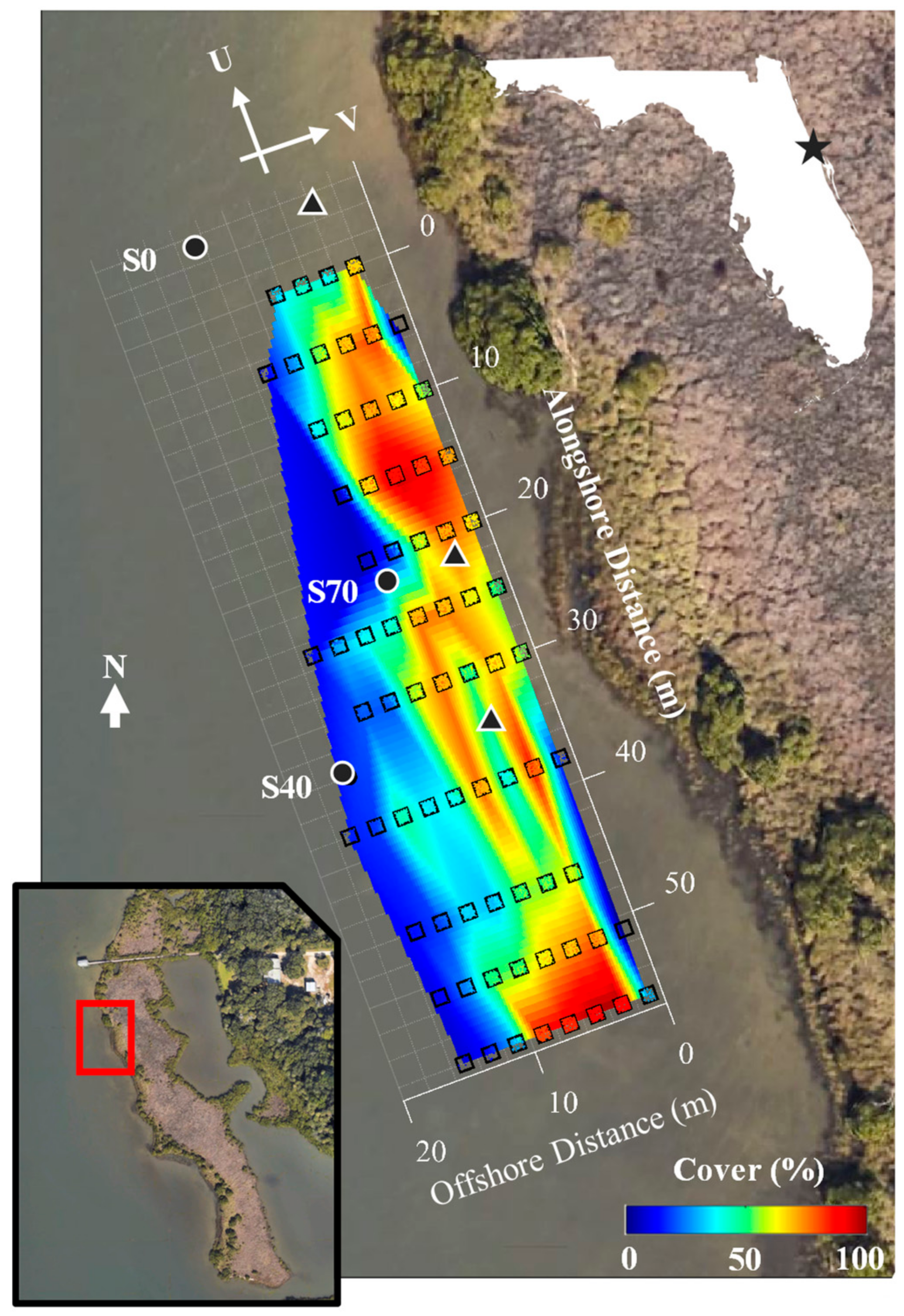
Hydrodynamic measurements and canopy characteristics were collected in the shallow (<1 m) waters of a submerged H. wrightii fringe late in the growing season (August). Seagrass cover within the fringe was characterized following transect methods applied to seagrass monitoring in Mosquito Lagoon, described in [32]. After identifying the northern extent of the patch (Figure 1), transects were established at 5 m intervals along the patch length (60 m), and cover was assessed for each 2 m transect length within a 1 m × 1 m quadrat separated into 10 × 10 cm squares. Two sample sites with variable seagrass cover, S40 (40% cover) and S70 (70% cover) (Figure 1), were selected for hydrodynamic study. Detailed seagrass density surveys were conducted at each site using a 10 × 10 cm quadrat, to assess the number, length, and width of all seagrass shoots and blades at each site (Table 1). The seagrass canopy height () was assumed equal to the mean blade length. An additional measurement location outside the seagrass patch (S0) was monitored as a hydrodynamic control. The S0 site was located at a comparable distance from shore 10 m upstream of the northernmost extent of the seagrass patch, where the benthic environment consisted of bare sediments.
2.2. Field Observations
At each site, current velocities were measured simultaneously nearshore in the seagrass canopy (~3 m from shore; water depth: 35–45 cm) and outside the seagrass patch in the main channel margin (10–15 m from shore; water depth: 43–64 cm). Nearshore velocity profiles (1 mm resolution) were sampled at 100 Hz using a Nortek (Rud, Norway) Vectrino Profiler, positioned such that the profile range fell between 2 and 5 cm above the bed. This placed the velocity profile largely within the seagrass canopy for both the S70 ( = 3.9 0.5 cm) and S40 (.6 0.8 cm) experiments, with the most accurate portion of the profile located at 4.0 and 3.5 cm above the bed, respectively. Velocity signals did not indicate hard returns (i.e., sporadic signal amplitude spikes) from vegetation interaction; thus, the clearing of vegetation from the probe vicinity was not necessary. Offshore channel velocities were measured within 30 cm of the bed (4 cm resolution) using a down-looking 2 MHz Nortek (Rud, Norway) Aquadopp HR Profiler (sample rate: 8 Hz), and measurement cells within 5 cm of the bottom (identified using signal amplitude profiles; [33]) were removed due to acoustic backscatter. Each velocimeter was deployed to sample at its maximum frequency to resolve turbulent velocity fluctuations at the smallest possible timescales. All velocimeters were aligned to a common coordinate system (Figure 1), such that U, V, and W correspond with streamwise (shore -parallel; positive with south-north ebb tide), cross-shore (positive onshore), and vertical velocity components, respectively. Onshore and offshore velocity profiles were collected continuously over four tidal cycles (~2 days) per site, with short (1–2 h) breaks during inclement weather (e.g., thunderstorms). This sampling window was chosen such that a wide range of tidal currents could be observed at each location, with extended sample times hindered by weather restrictions and instrument limitations (e.g., power and memory requirements).
Velocity data with poor quality control metrics were removed according to manufacturer recommendations, and mean velocity profiles were computed using time series averaged over 300 s of sampling (50% overlap). Mean offshore velocity profiles were used to estimate depth-integrated streamwise and cross-shore channel velocities (, ) using current speeds extrapolated over the bottommost 30 cm of the flow. Finally, channel-to-shore velocity attenuation was estimated for streamwise and cross-shore currents using depth integrated channel velocities and nearshore current speeds (, ) taken from the profile midpoint, with streamwise () and cross-shore () velocity attenuation defined as the best-fit slopes for the linear models and , respectively.
Local forcing conditions, including wind speeds (), wave heights (), and water depths, were measured continuously over each deployment. Wind speeds and directions were recorded at 2 m above the water surface (60-s interval) using a channel-deployed Davis Wind Speed and Direction Smart Sensor (S-WCF-M003; Onset, MA, USA). Sonic water surface loggers (XB Pro; Ocean Sensor Systems, FL, USA) deployed near each velocimeter were used to characterize onshore and offshore surface waves, where the standard deviation () of continuous 32 Hz water surface deformation time series was used to calculate the significant wave height () over 5 min (50% overlap) data segments (e.g., [34]). Estimates of nearshore and offshore depths were sourced from pressure loggers (U20L-04; Onset, MA, USA deployed approximately 100 m upstream of S0. Conversion to local depths was facilitated with on-site depth measurements collected at the start and end of each experiment.
2.3. Turbulence Data Analysis
Nearshore turbulence characteristics were estimated using 300 s (50% overlapped) turbulent velocity time series collected with the Nortek Vectrino Profiler. Time series were initially quality controlled by removing measurements with poor signal-to-noise ratios (SNR < 20) and low correlations (<80%), and the resulting gaps in the data series were replaced via linear interpolation. Each time series was then despiked using a phase-space thresholding algorithm [35,36] before being linearly detrended to remove the energy associated with the mean flow. On average, quality control procedures replaced less than 5% of the raw measurements for each 300 s data segment (<1000/30,000 points), and all time series where more than 15% of the data did not meet quality control standards were removed from analysis. For all analysis, it is assumed that the flow is stationary over each 5 min burst period.
Quality-controlled turbulent velocity time series were used to calculate wave-removed estimates of the Reynolds stress tensor. For each time segment, velocity fluctuations associated with surface waves and turbulence were separated using the phase method, which allows for wave-turbulence decomposition in spectral space [37]. After estimating the power spectral density function for a single velocity component (u, v, or w), the energy contributions due to waves and turbulence were separated using a best-fit line interpolated across the surface-wave frequency band, visually identified as 0.3 Hz < f < 2 Hz. Energy associated with waves and turbulence were then decoupled and used to calculate wave-removed estimates of the auto- (,,) and cross-correlation (,,) terms of the Reynolds stress tensor, as described in detail in [37]. Turbulence estimates were further refined by removing Doppler noise, which was identified and removed following the methods outlined in [38], developed explicitly for use with the Nortek Vectrino Profiler. For simplicity, all discussion of turbulence characteristics is limited to measurements collected in the most accurate portion of the profile located approximately 5 cm from the Vectrino instrument head (e.g., [38]). This corresponds to measurements collected at 3.9, 3.5, and 3.4 cm above the bed at the S70, S40, and S0 sites, respectively. Strong wave-induced fluctuations in the horizontal velocity components (, ) limited the accuracy of spectral decomposition and generated large biases in the squared terms for channel-wise () and cross-channel () turbulent energy (see discussion in [14]). Consequently, the following analysis is restricted to , , and , which contained less than 50% wave energy throughout the study. Wave-removed estimates of and were used to evaluate the Reynolds shear stress () and the shear turbulence production (), which were calculated as and , where and are the locally measured channel-wise and cross-channel vertical velocity gradients, respectively, and is the water density. Finally, calculated Reynolds stresses were used to estimate turbulent velocity scales (), such that .
The turbulent kinetic energy dissipation rate () was estimated from quality-controlled turbulence time series using a wave-corrected second order structure function method. Best-fit dissipation values were calculated using a least-squares approach following the procedure outlined in [39], with a burst-estimated Doppler noise [38] coefficient and a centered differencing scheme (e.g., [40]). Fits were conducted using velocity measurements centered in the near constant-noise portion of the sample volume (i.e., 5 cm from probe 7 mm), resulting in a total of 5 points used for each fit. Fits with adjusted R2 values less than 90% were rejected as erroneous. All turbulence metrics were additionally quality controlled by removing all 5 min data segments affected by boat wakes, which were noted from visual observations in the field and in the data.
3. Results
3.1. Site Characterization
Seagrass coverage was highly variable across the fringe, with percent cover ranging from 20 to 95% over the survey extent (Figure 1). All seagrasses present at the site were identified as shoal grass (Halodule wrightii), with no other apparent submerged aquatic vegetation. Measurements were spatially heterogeneous and patchy, with the highest coverage areas (90–95%) located approximately 5 m from shore and fringed by regions of comparatively lower cover (20–30%). Onsite observations suggested that the very nearshore region (1–2 m from shore) was completely devoid of live seagrass, likely driven by a combination of wave-induced bed shear and potential emergence over the tidal cycle. Mean vegetation heights were equivalent to the blade length for this seagrass species, with estimates of 3.90.5 cm (mean 95% CI) at S70 and 5.60.8 cm at the S40. Seagrass densities estimated at each site (Table 1) agreed well with bulk estimates of the local seagrass cover, with densities of 8300 and 4400 blades/m2 corresponding to coverage estimates of 70% and 40% at S70 and S40, respectively.
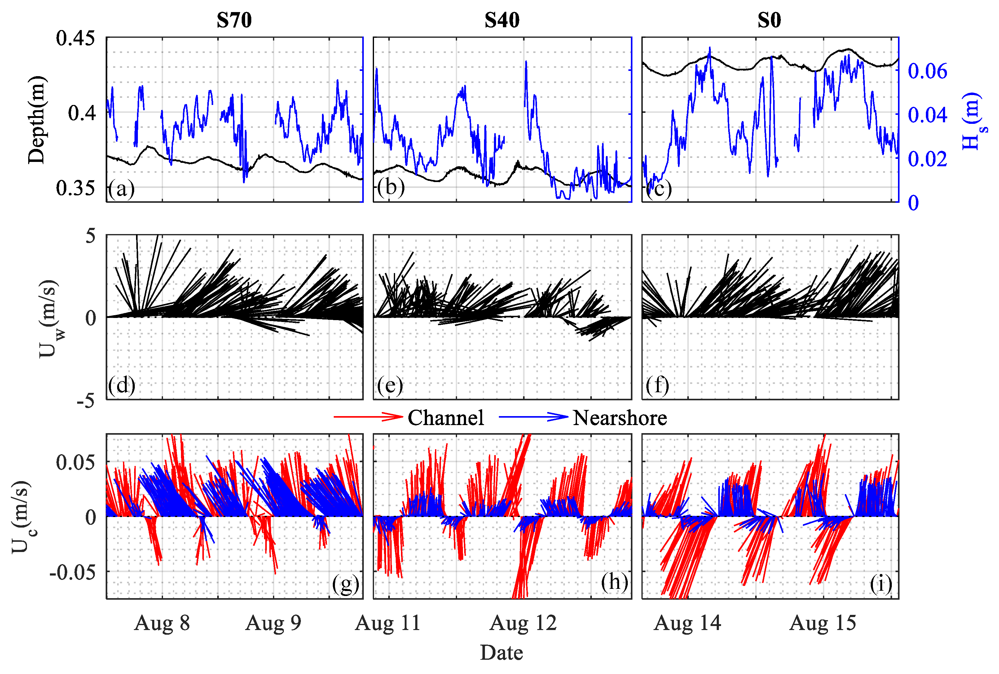
Hydrodynamic forcing was consistent across all three experiments (Figure 2). Winds were generally out of the southwest, with average wind speeds less than 3 m/s (Figure 2d–f). The prevailing wind drove waves towards the shore with significant wave heights of 3.40.1, 2.20.1, and 3.80.1 cm at S70, S40, and S0, respectively (Figure 2a–c). Measured water depths varied diurnally with the tide, which induced a local tidal amplitude of approximately 2 cm at the study site. Although all measurements were collected at similar distances from shore, local changes in bathymetry led to slightly larger water depths at the bare site (41.9 ± 0.1 cm) compared to those at the vegetated sites (S70: 36.0 ± 0.1 cm; S40: 35.6 ± 0.1 cm). This variability in depth is not expected to drive significant differences in near-bed hydrodynamics between sample locations.
Although the waves were small compared to other coastal environments, the shallow depths and weakly energetic current velocities associated with each sample location led to significant wave energy contributions in the total energy signal. Surface waves were identifiable in the majority of raw horizontal velocity time series (52%), with a period and wavelength (L) of 0.75–1.5 s and 0.9–2.5 m, respectively. Orbital velocity paths were elliptical (intermediate depth waves: L/20 < H < L/2; H: water depth), and wave-induced vertical velocity fluctuations () were typically much smaller than those induced by turbulence (< 0.5 for 80% of measurements). Estimates of the wave boundary layer height ([41]) suggest that was on the order of 1 mm, which is well below our sample volume and, more importantly, similar in scale to the sediment diameter at the sample site (84th percentile particle diameter: 0.5–1 mm). As such, we do not expect the waves to have a significant impact on the mean velocity magnitude or structure at our sample locations, where vegetation interactions and bed effects are anticipated to dominate the hydrodynamic roughness.
3.2. Current Velocities
Mean currents followed the tidal cycle, with directions that varied over flood (−) and ebb (+) tides and current magnitudes that were largest during peak tidal exchange (Figure 2g–i). Current magnitudes were generally larger in the channel ( = 4.50.1 cm/s) than along the adjacent shoreline, where mean current speeds varied by bed cover at each sample site (S70: 3.30.1 cm/s; S40: 1.10.1 cm/s; S0: 1.70.1 cm/s). Importantly, mean current speeds in the channel were similar across all three experiments (S70: 4.90.1 cm/s; S40: 4.40.2 cm/s; S0: 4.60.2 cm/s), suggesting that bulk forcing conditions remained consistent across the ~6 days of data collection. Tidal currents in the channel were symmetric, with statistically similar magnitudes observed during ebb tides (+: 4.50.1 cm/s) and flood tides (−: 4.50.2 cm/s). Tidal velocities were asymmetric at the nearshore monitoring stations, where north–south (i.e., flood tide) velocities were directionally sporadic and nearly 50% lower than ebb tide currents.
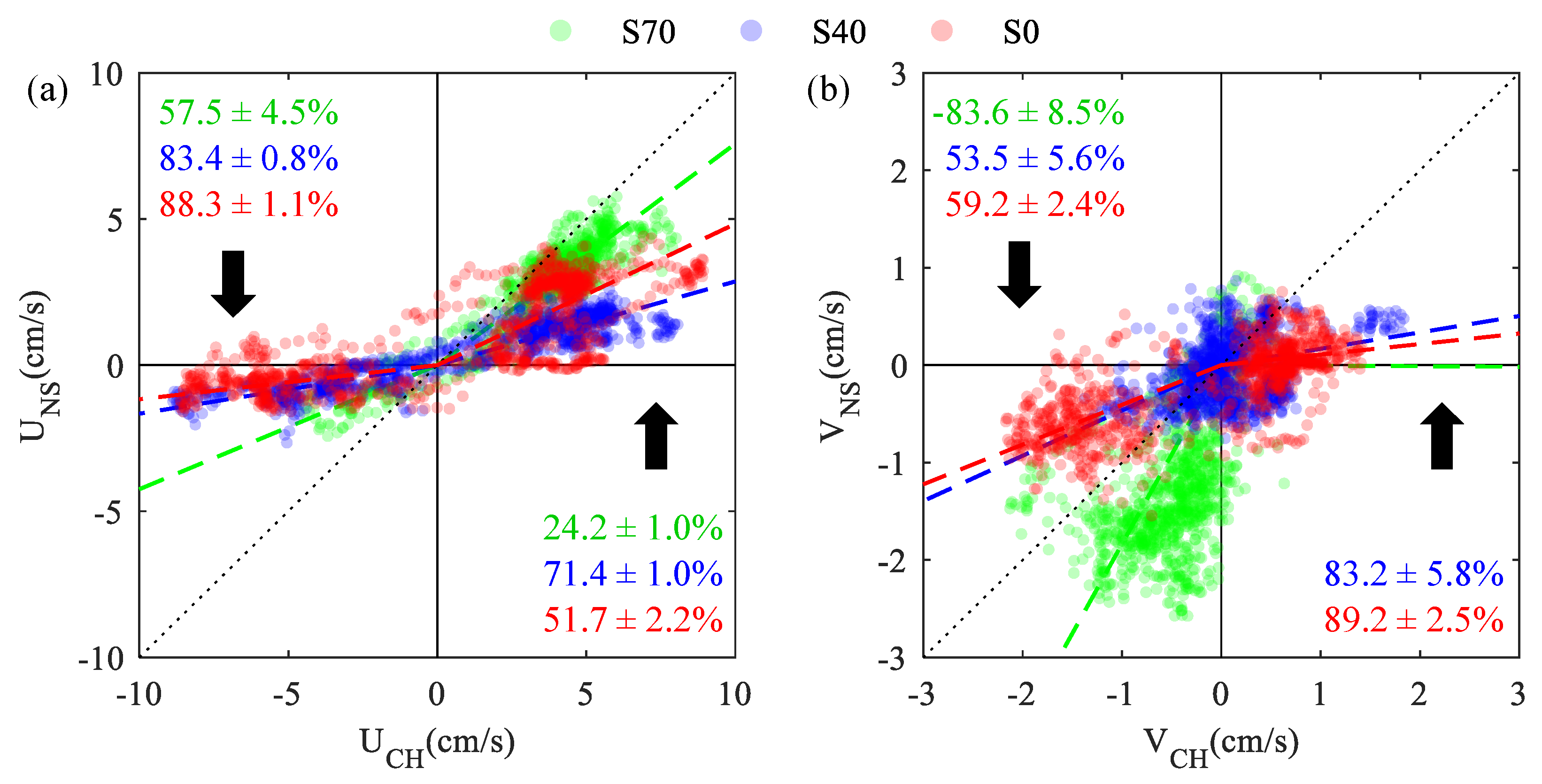
Channel velocities were attenuated near the shore at each site, but significant differences in channel-to-shore velocity attenuation (,) were observed across sample locations and tidal stages (Figure 3). Alongshore currents () were most strongly attenuated over the tidal flood stage (: 58–90%), with diminished attenuation rates (: 24–71%) observed over ebb tide. Although alongshore attenuation rates were higher at S40 71.4 1.0%) than over bare sediment 51.7 2.2%) during ebb flows, attenuation rates at S70 were surprisingly low 24.2 1.0%). This lack of attenuation at the denser seagrass site was especially pronounced for cross-shore flows (), where velocity measurements nearshore were nearly twice as large as those observed in the channel ( = 1.81 0.08). These trends are also apparent in Figure 2g, where observed velocity vectors show that nearshore ebb flows had consistently high magnitudes () and directional shifts offshore at S70.
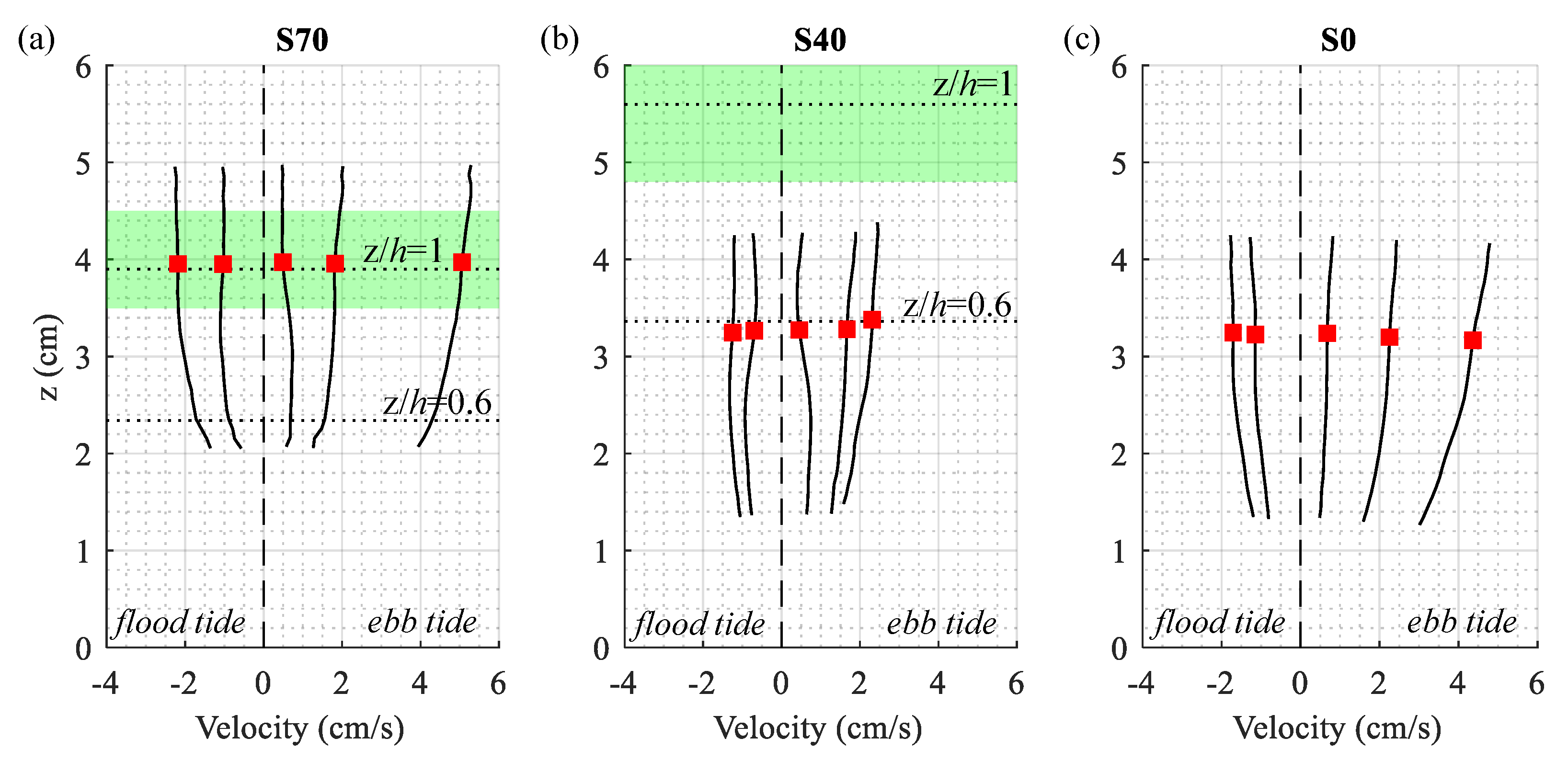
Mean horizontal velocity profiles () measured nearshore over the tidal cycle (Figure 4) followed typical boundary layer structures, with maximum velocity shear near the bed and current speeds that increased with distance above the sediment surface. High current speeds at S70 and S0 drove strong benthic velocity shear, with mean velocity differences as large as 2 cm/s recorded over the 3 cm sample volume. While velocity profiles were collected in similar positions relative to the bed (~2–5 cm above bottom), site-scale differences in canopy height produced data from different canopy positions at S40 and S70. Velocity profiles at the more sparsely vegetated site (S40) were measured entirely within the seagrass canopy (0.25 < z/ < 0.75), while profiles at the more densely vegetated site (S70) extended from within to above the canopy (0.55 < z/ < 1.25). All velocity profiles approached zero near the bed, consistent with the no-slip condition at the sediment-water interface. Importantly, non-zero flow velocities were observed throughout the seagrass canopy at both S40 and S70, with non-zero significant velocity shear at all measurement elevations.
3.3. Turbulence Characteristics
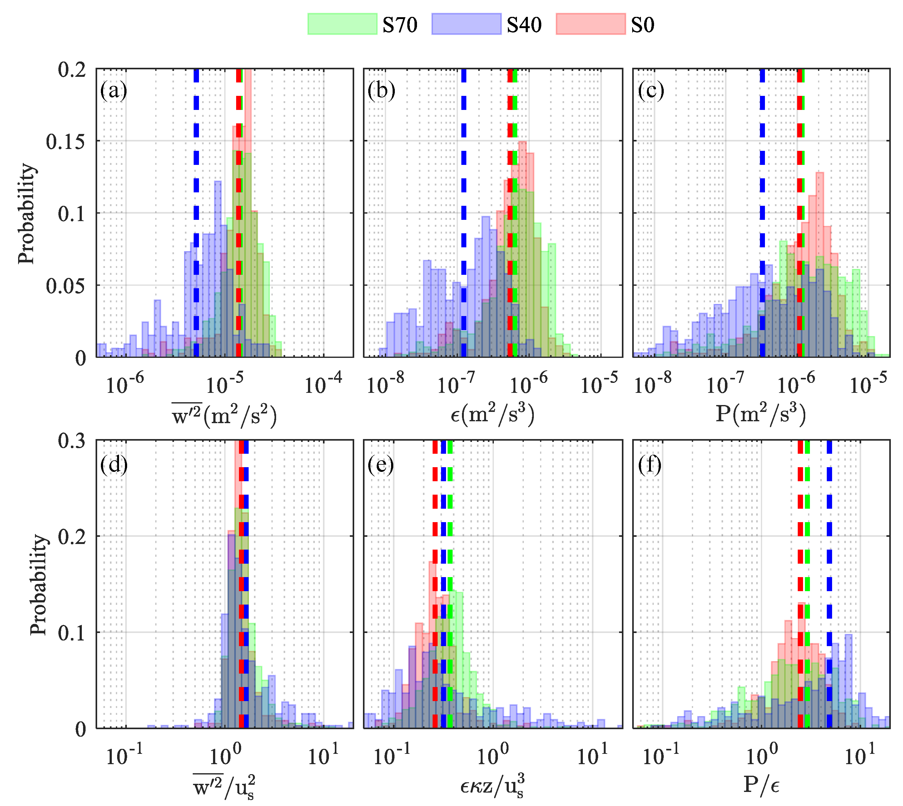
Nearshore turbulence characteristics (, , ) varied with the local velocity such that the strongest mixing was observed at the most tidally energetic sample sites (Figure 5). Turbulent energy (; Figure 5a) estimates were nearly twice as large at S70 (1.30.05 × 10−5 m2/s2) and S0 (1.10.05 × 10−5 m2/s2) than at S40 (5.20.03 × 10−6 m2/s2), where weak velocities resulted in decreased mixing. Turbulent kinetic energy dissipation rates (; Figure 5b) varied tidally from 10−8 to 10−6 m2/s3, with significantly weaker (~70–80%) dissipation observed at the sparse site (mean: 1.1 × 10⁻⁷ m2/s3) than at the dense or bare sites. Turbulent energy and dissipation rate both scaled well with the local turbulent velocity scales (; Figure 5d,e), and normalized means collapsed (within an order) to 0.3 (= 0.41) and / 0.2. The highest turbulent shear production rates (; Figure 5c) were observed at S70 (7.0 × 10⁻⁷ m2/s3), where estimates were 2–7 × larger than those calculated at S40 or S0, respectively. Average production-to-dissipation ratios were O(1) at all three sample locations (mean: = 1.81), suggesting that shear production and dissipation were approximately balanced. Importantly, individual estimates were largest at the more sparsely vegetated site (S40), where production was over five times larger than dissipation for 40% of all measurements.
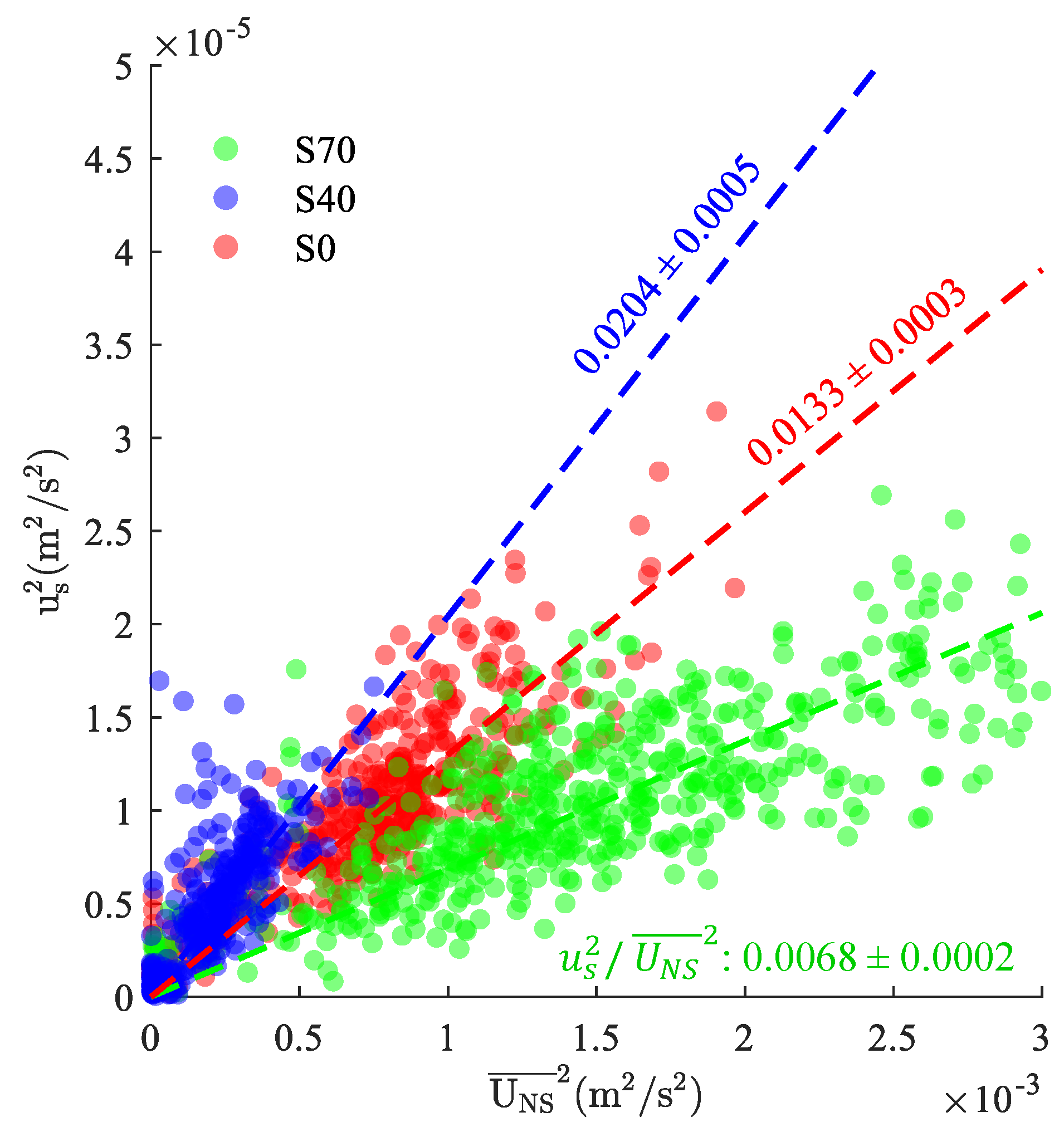
Normalized velocity scales () were used to investigate the variability of measured turbulence characteristics with current velocities at each study site (Figure 6). Although is analogous to the more widely reported boundary drag coefficient (i.e., ), it does not necessarily scale with the local bed shear stress (), which would require a priori assumptions about the vertical distribution of near the bed (e.g., [42]). Squared velocity scales varied linearly with the square of the local current velocity, and increased current speeds were associated with elevated turbulence levels. The mean ratio of , represented by the best-fit lines shown in Figure 5, varied by sample location, with estimates of 0.00680.0002, 0.02040.0005, and 0.01330.0003 at S70, S40, and S0, respectively. Normalized velocity scales demonstrated some Reynolds number dependence (not shown), with estimates that were several orders of magnitude larger (S70: 0.130.07; S40: 0.170.09; S0: 1.571.18) at the lowest flow speeds (< 5 mm/s). Similar current speed dependencies have been observed for the drag coefficient and friction factor in weakly energetic boundary layers, where increases in the apparent drag are often attributed to viscous effects [43] and/or unsteadiness [44]. In the current study, a lack of high quality (i.e., wave-free) data at low flow speeds precluded robust analyses of Reynolds number dependencies, and additional discussion is considered beyond the scope of this manuscript.
4. Discussion
4.1. Submerged Canopy Classification
Hydrodynamic characteristics for flows through submerged vegetation are largely set by the canopy density, with limits on flow behavior determined by the relative importance of canopy drag, which dominates in dense vegetation, and bed drag, which dominates in sparse vegetation [9]. Flows through dense vegetation are heavily influenced by the canopy itself, with strong velocity attenuation and weak mixing near the bed and a turbulently energetic canopy shear layer (e.g., [45]). Flows through sparse vegetation, on the other hand, are almost entirely dominated by bed interactions, with nearly logarithmic velocity profiles and stem/blade-scale turbulence that enhances bed-generated mixing locally (e.g., [19]). For simple stem morphologies, vegetation can be described at the canopy scale using the frontal area per volume () and the frontal area index (), where is the number of the blades per bed area and is the characteristic stem or blade width [29]. A canopy can be categorized as either sparse ( 0.1) or dense ( 0.1) using measurements of the vegetation and canopy drag coefficient (), which is typically taken as [46]. When 0.1, the canopy is considered transitional, with hydrodynamics influenced by both bottom roughness and differential flow drag at the top of the canopy [21]. Notably, for dense and transitional canopies capable of producing shear-layer vortices (> 0.1), the distance that canopy-induced shear is able to penetrate below the canopy surface can be estimated as = [0.23 0.06]/ [47].
In the current study, both vegetated sample sites were classified as transitional (), with frontal area indices () of 0.14 and 0.32 at S40 and S70, respectively (Table 1). This classification was consistent with hydrodynamic observations at each sample site, which highlighted the presence of both velocity shear and turbulence within the seagrass canopy. Results agreed well with other studies of transitional and sparse canopy flows, which are often characterized by moderate current speeds and energetic mixing near the bed within the canopy [19,29]. Calculated penetration length scales (; Table 1) show that the canopy shear layer extended over most of the canopy height and throughout the measurement volume for both deployments (S40: 9.22.4 cm; S70: 2.80.7 cm). This deep penetration of canopy-induced shear helps explain the shape of the velocity profiles measured at S40 and S70 (Figure 4), which lacked the mid-profile inflection point often observed in flows through dense and transitional canopies (e.g., [48,49]). Although current speeds were not resolved throughout the canopy, velocity profiles at S70 showed evidence of a potential canopy shear layer near the bottom of the measurement volume, where velocities sharply decreased at an elevation consistent with the penetration length scale ( − 1 cm above the bottom). Conversely, the vertical structure of velocity profiles at S40, where the canopy shear layer penetrated to the bed, more closely matched that observed at S0, and log-fit roughness heights (, e.g., [44]) at both sites (not shown; 2 mm) suggested that the near-bed structure of velocity profiles was set by sediment characteristics rather than canopy-induced shear.
4.2. Mean Flow Variability
Although hydrodynamic observations at S40 and S70 were qualitatively similar to transitionally dense canopy flow models, comparisons to the unvegetated control site (S0) suggest that flows behaved very differently at each location. This is perhaps most apparent in the differential effects of the seagrass canopy on the mean flow. While the sparser seagrass site (S40) was associated with slightly enhanced near-bed flow attenuation, as predicted for flows through vegetation [45], observations at the more densely vegetated site (S70) defied predictions. Alongshore velocities were only marginally reduced in the seagrass fringe at S70, and cross-shore flows were appreciably stronger than flows outside of the vegetation, with dramatic offshore current steering that was not apparent at any other sample location. These differences are interesting in that they run counter to canopy flow theory and intuition. Assuming forcing conditions are comparable and measurements are collected from similar positions within the canopy, it is expected that increased canopy density (i.e., increased ) should drive increased flow attenuation and decreased velocity shear near the bed [19]. While velocity measurements at S40 and S70 were positioned at slightly different locations within the canopy (z/= 0.6 and 1, respectively), they were both collected within the canopy shear layer and at similar heights above the bottom. The relative influence of bed and canopy drag should be similar across sites, and differences in hydrodynamic observations cannot be attributed to canopy position alone. Variability in flow attenuation and current direction also cannot be linked to radically different forcing conditions or flow generation mechanisms (e.g., wave pumping: [28]; return flow: [50]), since conditions remained fairly constant across experiments and wind/wave and current directions were typically opposed (Figure 2).
We hypothesize that the observed flow steering and acceleration at S70 were caused by within-patch heterogeneity of the seagrass fringe. Although S70 was located in a locally dense region of seagrass, it was also positioned in the narrowest portion of the fringe. Strong offshore currents were most prevalent during ebb tide (+), suggesting that flows between the fringe and the shoreline may have been funneled through this area of the seagrass canopy, which likely offered lower resistance (i.e., [48]) than the more densely vegetated region to the north (Figure 1). This type of preferential flow path behavior has been observed in studies of flow through vegetation [51,52], and other authors have commented on the potential importance of vegetation clustering and patch heterogeneity for defining appropriate spatial averaging scales in flows through submerged vegetation [45,53]. In this study, the point measurements at S40 and S70 show that within-patch turbulence and momentum fluxes vary dramatically across relatively small spatial scales (~20 m separation distance) and that fringe-scale averaging may not capture important canopy physics. Although this spatial variability is likely less important for characterizations of estuary or reach scale vegetation drag (e.g., [45]), it may have significant implications for patch scale nutrient uptake [54], sediment transport [55], and patch stability [56], which are all heavily dependent on the magnitude of mean flow and turbulence within the submerged canopy. Notably, observed changes in the flow direction also provide a potential link between the inland marsh and the offshore channel, a path which may otherwise be blocked or throttled by seagrass along the shoreline.
4.3. Turbulence Budget and Velocity Scales
Observed turbulence characteristics shed light on the relative importance of turbulent shear and stem production at each sample site. There are two sources of turbulence in submerged canopy flows: (1) shear production () generated by velocity shear near the bed and canopy surface, and (2) stem production () generated in the wakes of individual seagrass blades or stems. For fully developed canopy flows, turbulent kinetic energy dissipation () is expected to be balanced by the sum of shear and stem production, such that [20]. However, in the current study, dissipation was well balanced by shear production alone (; Figure 5), suggesting that stem production played a minor role in turbulence generation at S40 or S70. Near bed turbulence was instead dominated by strong velocity shear induced at the bed and canopy surface. The relatively low vegetation density allowed the canopy shear layer to contribute to mixing throughout the canopy, although the formation of a persistent and coherent shear layer at the canopy surface may have been hindered by the sparseness and heterogeneity of the seagrass fringe [19]. Sporadically high production-to-dissipation ratios ( 5) at the vegetated sites, especially S40, imply that the vertical diffusion and advection of turbulence may have been transiently important in the seagrass fringe, as has been reported in previous studies of flows through spatially heterogeneous canopies (e.g., [57]).
Normalized velocity scales (; Figure 6) were similar to previous reports of normalized Reynolds stresses in submerged vegetation canopies. For instance, Lacy and Wyllie-Echeverria [19] and Hansen and Reidenbach [14] both reported normalized Reynolds stresses on the order of 0.01 in varying density seagrass meadows, although the relevant normalization velocities were taken as the difference between within and above canopy current speeds () and ambient above canopy velocities (), respectively. More importantly, both studies reported decreases in normalized Reynolds stresses with increasing seagrass densities, as observed in the current work. Lacy and Wyllie-Echeverria [19] attributed this trend to sheltering in dense canopies, where smaller stem-spacing and weaker currents reduce the importance of multiple-element flow interactions. Direct comparisons across sample sites were complicated by the choice of normalization velocity (), which was necessitated by the sampling strategy used in the current work. This was most evident in comparisons between the vegetated and bare sample sites, where enhancements were observed above bare sediment (S0) in comparison to the most densely vegetated sample site (S70). Although this may have been related to canopy sheltering (see above), it seems likely that the mean velocities used for normalization represent fundamentally different scales at both sites, especially considering the discrepancy in measurement locations (i.e., outside vs. within the canopy). As such, we emphasize that ratios at S0 are included for reference but should not be considered directly comparable to estimates made at S40 and/or S70.
5. Conclusions
The mean flow and turbulence observations presented in this manuscript are some of the first such measurements reported for submerged shoal grass (H. wrightii) canopies, with important implications for sediment and nutrient fluxes in shallow coastal estuaries. Experiments were conducted near the bed (~4 cm above bottom) in a narrow (~15 m wide) seagrass fringe, where hydrodynamic measurements were used to assess the effects of a shoal grass canopy on near-bed flow (i.e., velocity attenuation) and mixing (, , etc.) characteristics. Measurements were collected within the canopy for relatively dense (70%) and sparse (40%) vegetation, with reference measurements collected near the bed above bare sediment. Shear induced at the canopy surface was able to penetrate deep within the canopy at both vegetated sites, generating significant velocity shear and turbulence near the bed. This velocity shear dominated the turbulence budget for both sparse and dense canopy flows (), suggesting that stem production was relatively unimportant in the studied seagrass fringe. The sparsely vegetated sample site was associated with an increase in channel-to-shore velocity attenuation relative to flows above bare sediment, but strong offshore-oriented currents were observed within the denser vegetation canopy, implying that flow was steered and accelerated through the shoal grass patch. Importantly, these results suggest that patch-scale heterogeneity has significant consequences for transport within and across seagrass fringes.
As key habitat units separating open channels from intertidal shoreline areas, submerged vegetation fringes are particularly important to the habitat structure, ecological function, and geomorphic stability of shoreline ecotones. This work is among the first studies on the hydrodynamic effects of fringe seagrass meadows, and the results suggest that canopy density and its distribution are likely influential to the nearshore environment. Although seagrass fringes may attenuate flows and stabilize benthic sediments at large scales (i.e., channels and reaches), we show that spatial variations in canopy density may create regions of enhanced hydraulic connectivity between the channel and marsh platform, providing pathways for nutrient fluxes and potential avenues for sediment erosion and canopy degradation caused by enhanced near-bed mixing. While incorporation of fringe meadows, for instance, as natural features in living shoreline stabilization designs, likely benefits geomorphic stability along the shoreline, more study is needed to quantify the effects of patch distribution on nearshore sediment transport and retention.
Author Contributions
Conceptualization, K.K. and V.K.; methodology, D.C.; formal analysis, D.C.; investigation, K.K. and V.K.; resources, K.K.; data curation, K.K. and V.K.; writing—original draft preparation, D.C.; writing—review and editing, D.C., K.K., and V.K.; visualization, D.C.; supervision, K.K.; project administration, K.K.; funding acquisition, K.K. All authors have read and agreed to the published version of the manuscript.
Funding
This research was funded by the U.S. National Science Foundation (NSF grants #1617374 and #1944880) and the University of Central Florida.
Data Availability Statement
The data presented in this study are available on request from the corresponding author.
Acknowledgments
We would like to thank the Canaveral National Seashore for their support and use of the Feller’s House Research Station. We also thank Arash Aliabadi Farahani, Sam Maldonado, and Iris Peterson for field assistance and Melinda Donnelly for discussions related to seagrass characterization.
Conflicts of Interest
The authors declare no conflict of interest.
References
- Touchette, B.W.; Burkholder, J.A.M. Overview of the physiological ecology of carbon metabolism in seagrasses. J. Exp. Mar. Biol. Ecol. 2000, 250, 169–205. [Google Scholar] [CrossRef]
- McGlathery, K.; Sundbäck, K.; Anderson, I. Eutrophication in shallow coastal bays and lagoons: The role of plants in the coastal filter. Mar. Ecol. Prog. Ser. 2007, 348, 1–18. [Google Scholar] [CrossRef] [Green Version]
- Christianen, M.J.A.; van Belzen, J.; Herman, P.M.J.; van Katwijk, M.M.; Lamers, L.P.M.; van Leent, P.J.M.; Bouma, T.J. Low-Canopy Seagrass Beds Still Provide Important Coastal Protection Services. PLoS ONE 2013, 8, e62413. [Google Scholar]
- Jackson, E.L.; Rowden, A.A.; Attrill, M.J.; Bossey, S.J.; Jones, M.B. The importance of seagrass beds as a habitat for fishery species. Oceanogr. Mar. Biol. 2001, 39, 269–304. [Google Scholar]
- Coll, M.; Schmidt, A.; Romanuk, T.; Lotze, H.K. Food-Web Structure of Seagrass Communities across Different Spatial Scales and Human Impacts. PLoS ONE 2011, 6, e22591. [Google Scholar] [CrossRef] [PubMed] [Green Version]
- Duarte, C.M.; Marbà, N.; Gacia, E.; Fourqurean, J.W.; Beggins, J.; Barrón, C.; Apostolaki, E.T. Seagrass community metabolism: Assessing the carbon sink capacity of seagrass meadows. Glob. Biogeochem. Cycles 2010, 24, 24. [Google Scholar] [CrossRef] [Green Version]
- Van Katwijk, M.M.; Thorhaug, A.; Marbà, N.; Orth, R.J.; Duarte, C.M.; Kendrick, G.A.; Althuizen, I.H.J.; Balestri, E.; Bernard, G.; Cambridge, M.L.; et al. Global analysis of seagrass restoration: The importance of large-scale planting. J. Appl. Ecol. 2016, 53, 567–578. [Google Scholar] [CrossRef] [Green Version]
- Lee, K.-S.; Park, S.R.; Kim, Y.K. Effects of irradiance, temperature, and nutrients on growth dynamics of seagrasses: A review. J. Exp. Mar. Biol. Ecol. 2007, 350, 144–175. [Google Scholar] [CrossRef]
- Nepf, H.M. Hydrodynamics of vegetated channels. J. Hydraul. Res. 2012, 50, 262–279. [Google Scholar] [CrossRef] [Green Version]
- Koch, E.W. Hydrodynamics, diffusion-boundary layers and photosynthesis of the seagrasses Thalassia testudinum and Cymodocea nodosa. Mar. Biol. 1994, 118, 767–776. [Google Scholar] [CrossRef]
- De Boer, W.F. Seagrass-sediment interactions, positive feedbacks and critical thresholds for occurrence: A review. Hydrobiologia 2007, 591, 5–24. [Google Scholar] [CrossRef]
- Hurd, C.L. Water Motion, Marine Macroalgal Physiology, and Production. J. Phycol. 2000, 36, 453–472. [Google Scholar] [CrossRef] [PubMed]
- Rheuban, J.E.; Berg, P.; McGlathery, K.J. Ecosystem metabolism along a colonization gradient of eelgrass (Zostera marina) measured by eddy correlation. Limnol. Oceanogr. 2014, 59, 1376–1387. [Google Scholar] [CrossRef] [Green Version]
- Hansen, J.C.R.; Reidenbach, M.A. Turbulent mixing and fluid transport within Florida Bay seagrass meadows. Adv. Water Resour. 2017, 108, 205–215. [Google Scholar] [CrossRef]
- Peterson, C.; Luettich, R.; Micheli, F.; Skilleter, G. Attenuation of water flow inside seagrass canopies of differing structure. Mar. Ecol. Prog. Ser. 2004, 268, 81–92. [Google Scholar] [CrossRef]
- Fonseca, M.S.; Cahalan, J.A. A preliminary evaluation of wave attenuation by four species of seagrass. Estuar. Coast. Shelf Sci. 1992, 35, 565–576. [Google Scholar] [CrossRef]
- Bradley, K.; Houser, C. Relative velocity of seagrass blades: Implications for wave attenuation in low-energy environments. J. Geophys. Res. Earth Surf. 2009, 114. [Google Scholar] [CrossRef]
- Ghisalberti, M.; Nepf, H. The Structure of the Shear Layer in Flows over Rigid and Flexible Canopies. Environ. Fluid Mech. 2006, 6, 277–301. [Google Scholar] [CrossRef]
- Lacy, J.R.; Wyllie-Echeverria, S. The influence of current speed and vegetation density on flow structure in two macrotidal eelgrass canopies. Limnol. Oceanogr. Fluids Environ. 2011, 1, 38–55. [Google Scholar] [CrossRef]
- Zhang, J.; Lei, J.; Huai, W.; Nepf, H. Turbulence and Particle Deposition Under Steady Flow Along a Submerged Seagrass Meadow. J. Geophys. Res. Oceans 2020, 125, 125. [Google Scholar] [CrossRef]
- Nepf, H.M. Flow and Transport in Regions with Aquatic Vegetation. Annu. Rev. Fluid Mech. 2012, 44, 123–142. [Google Scholar] [CrossRef] [Green Version]
- Luhar, M.; Infantes, E.; Nepf, H. Seagrass blade motion under waves and its impact on wave decay. J. Geophys. Res. Oceans 2017, 122, 3736–3752. [Google Scholar] [CrossRef] [Green Version]
- Adhitya, A.; Bouma, T.; Folkard, A.; van Katwijk, M.; Callaghan, D.; de Iongh, H.; Herman, P. Comparison of the influence of patch-scale and meadow-scale characteristics on flow within seagrass meadows: A flume study. Mar. Ecol. Prog. Ser. 2014, 516, 49–59. [Google Scholar] [CrossRef] [Green Version]
- El Allaoui, N.; Serra, T.; Colomer, J.; Soler, M.; Casamitjana, X.; Oldham, C. Interactions between Fragmented Seagrass Canopies and the Local Hydrodynamics. PLoS ONE 2016, 11, e0156264. [Google Scholar] [CrossRef] [PubMed]
- Yang, J.Q.; Nepf, H.M. Impact of Vegetation on Bed Load Transport Rate and Bedform Characteristics. Water Resour. Res. 2019, 55, 6109–6124. [Google Scholar] [CrossRef]
- Tinoco, R.O.; San Juan, J.E.; Mullarney, J.C. Simplification bias: Lessons from laboratory and field experiments on flow through aquatic vegetation. Earth Surf. Process. Landf. 2020, 45, 121–143. [Google Scholar] [CrossRef]
- Hansen, J.C.R.; Reidenbach, M.A. Seasonal Growth and Senescence of a Zostera marina Seagrass Meadow Alters Wave-Dominated Flow and Sediment Suspension Within a Coastal Bay. Estuaries Coasts 2013, 36, 1099–1114. [Google Scholar] [CrossRef]
- Luhar, M.; Infantes, E.; Orfila, A.; Terrados, J.; Nepf, H.M. Field observations of wave-induced streaming through a submerged seagrass (Posidonia oceanica) meadow. J. Geophys. Res. Oceans 2013, 118, 1955–1968. [Google Scholar] [CrossRef] [Green Version]
- Luhar, M.; Rominger, J.; Nepf, H. Interaction between flow, transport and vegetation spatial structure. Environ. Fluid Mech. 2008, 8, 423–439. [Google Scholar] [CrossRef]
- Morris, L.J.; Virnstein, R.W. The demise and recovery of seagrass in the northern Indian River Lagoon, Florida. Estuaries 2004, 27, 915–922. [Google Scholar] [CrossRef]
- Virnstein, R.W.; Steward, J.S.; Morris, L.J. Seagrass coverage trends in the Indian River Lagoon system. Fla. Sci. 2007, 70, 397–404. [Google Scholar]
- Morris, L.J.; Virnstein, R.W.; Miller, J.D.; Hall, L.M. Monitoring Seagrass in Indian River Lagoon, Florida Using Fixed Transects. In Seagrasses: Monitoring, Ecology, Physiology, and Managment; Bortone, S.A., Ed.; CRC Press: Boca Raton, FL, USA, 2000; pp. 167–176. [Google Scholar]
- Kibler, K.M.; Kitsikoudis, V.; Donnelly, M.; Spiering, D.W.; Walters, L. Flow-Vegetation Interaction in a Living Shoreline Restoration and Potential Effect to Mangrove Recruitment. Sustainability 2019, 11, 3215. [Google Scholar] [CrossRef] [Green Version]
- Dean, R.G.; Dalrymple, R.A. Water Wave Mechanics for Engineers and Scientists. In Advanced Series on Ocean Engineering; World Scientific Publishing Co.: Singapore, 1991. [Google Scholar]
- Goring, D.G.; Nikora, V.I. Despiking Acoustic Doppler Velocimeter Data. J. Hydraul. Eng. 2002, 128, 117–126. [Google Scholar] [CrossRef] [Green Version]
- Wahl, T.L. Discussion of “Despiking acoustic doppler velocimeter data” by Derek G. Goring and Vladimir I. Nikora. J. Hydraul. Eng. 2003, 129, 484–487. [Google Scholar] [CrossRef] [Green Version]
- Bricker, J.D.; Monismith, S.G. Spectral wave-turbulence decomposition. J. Atmos. Ocean. Technol. 2007, 24, 1479–1487. [Google Scholar] [CrossRef]
- Thomas, R.E.; Schindfessel, L.; McLelland, S.J.; Creëlle, S.; De Mulder, T. Bias in mean velocities and noise in variances and covariances measured using a multistatic acoustic profiler: The Nortek Vectrino Profiler. Meas. Sci. Technol. 2017, 28, 075302. [Google Scholar] [CrossRef]
- Scannell, B.D.; Rippeth, T.P.; Simpson, J.H.; Polton, J.A.; Hopkins, J.E. Correcting Surface Wave Bias in Structure Function Estimates of Turbulent Kinetic Energy Dissipation Rate. J. Atmos. Ocean. Technol. 2017, 34, 2257–2273. [Google Scholar] [CrossRef]
- Wiles, P.J.; Rippeth, T.P.; Simpson, J.H.; Hendricks, P.J. A novel technique for measuring the rate of turbulent dissipation in the marine environment. Geophys. Res. Lett. 2006, 33, 33. [Google Scholar] [CrossRef]
- Zai-Jin, Y. A simple model for current velocity profiles in combined wave-current flows. Coast. Eng. 1994, 23, 289–304. [Google Scholar] [CrossRef]
- Egan, G.; Cowherd, M.; Fringer, O.; Monismith, S. Observations of Near-Bed Shear Stress in a Shallow, Wave- and Current-Driven Flow. J. Geophys. Res. Oceans 2019, 124, 6323–6344. [Google Scholar] [CrossRef]
- Ligrani, P.M.; Moffat, R.J. Structure of transitionally rough and fully rough turbulent boundary layers. J. Fluid Mech. 1986, 162, 69. [Google Scholar] [CrossRef]
- Cannon, D.J.; Troy, C.D. Observations of turbulence and mean flow in the low-energy hypolimnetic boundary layer of a large lake. Limnol. Oceanogr. 2018, 63, 2762–2776. [Google Scholar] [CrossRef] [Green Version]
- Nepf, H.; Ghisalberti, M. Flow and transport in channels with submerged vegetation. Acta Geophys. 2008, 56, 753–777. [Google Scholar] [CrossRef]
- Nepf, H.M. Flow Over and Through Biota. In Treatise on Estuarine and Coastal Science; Elsevier: Amsterdam, The Netherlands, 2012; Volume 2, pp. 267–288. [Google Scholar]
- Nepf, H.; Ghisalberti, M.; White, B.; Murphy, E. Retention time and dispersion associated with submerged aquatic canopies. Water Resour. Res. 2007, 43, 43. [Google Scholar] [CrossRef]
- Fonseca, M.S.; Koehl, M.A.R. Flow in seagrass canopies: The influence of patch width. Estuarine Coast. Shelf Sci. 2006, 67, 1–9. [Google Scholar] [CrossRef]
- Hendriks, I.E.; Bouma, T.J.; Morris, E.P.; Duarte, C.M. Effects of seagrasses and algae of the Caulerpa family on hydrodynamics and particle-trapping rates. Mar. Biol. 2010, 157, 473–481. [Google Scholar] [CrossRef]
- Masselink, G.; Black, K.P. Magnitude and cross-shore distribution of bed return flow measured on natural beaches. Coast. Eng. 1995, 25, 165–190. [Google Scholar] [CrossRef]
- Etminan, V.; Lowe, R.J.; Ghisalberti, M. A new model for predicting the drag exerted by vegetation canopies. Water Resour. Res. 2017, 53, 3179–3196. [Google Scholar] [CrossRef]
- Kitsikoudis, V.; Yagci, O.; Kirca, V.S.O. Experimental analysis of flow and turbulence in the wake of neighboring emergent vegetation patches with different densities. Environ. Fluid Mech. 2020, 20, 1417–1439. [Google Scholar] [CrossRef]
- Horstman, E.M.; Bryan, K.R.; Mullarney, J.C.; Pilditch, C.A.; Eager, C.A. Are flow-vegetation interactions well represented by mimics? A case study of mangrove pneumatophores. Adv. Water Resour. 2018, 111, 360–371. [Google Scholar] [CrossRef]
- Thomas, F.I.M.; Cornelisen, C.D.; Zande, J.M. Effects of water velocity and canopy morphology on ammonium uptake by seagrass communities. Ecology 2000, 81, 2704–2713. [Google Scholar] [CrossRef]
- Donatelli, C.; Ganju, N.K.; Fagherazzi, S.; Leonardi, N. Seagrass Impact on Sediment Exchange Between Tidal Flats and Salt Marsh, and The Sediment Budget of Shallow Bays. Geophys. Res. Lett. 2018, 45, 4933–4943. [Google Scholar] [CrossRef] [Green Version]
- Duarte, C.M.; Fourqurean, J.W.; Krause-Jensen, D.; Olesen, B. Dynamics of Seagrass Stability and Change. In Seagrasses: Biology, Ecology and Conservation; Springer: Dordrecht, The Netherlands, 2006; pp. 271–294. [Google Scholar]
- Kitsikoudis, V.; Kibler, K.M.; Walters, L.J. In-situ measurements of turbulent flow over intertidal natural and degraded oyster reefs in an estuarine lagoon. Ecol. Eng. 2020, 143, 105688. [Google Scholar] [CrossRef]
Figure 1.
Site map and observed seagrass densities. The relative location of each deployment (S0, S40, S70) is indicated (circles: Aquadopp HR; triangles: Vectrino), along with a colormap indicating the local seagrass cover. Seagrass was observed south of the surveyed region, but not surveyed in detail. The channelwise () and cross-shore () velocity convention is included for reference. The inset map shows the survey location along the shoreline of Mosquito Lagoon (Florida, USA: white outline), including a dock approximately 75 m north of the northernmost sample location.

Figure 2.
Overview of water depths (black line; a–c), wave heights (blue line; a–c), wind speeds (d–f), and current speeds (blue: nearshore and red: channel; g–i) observed over each deployment in 2019. Wind and current speeds are displayed as quiver plots, with the length of the line representing the measurement magnitude and the direction of the line indicating the flow direction referenced to the local definition of channelwise (U) and cross-shore (V) flow (see Figure 1). Water depths were measured nearshore in the vicinity of the Vectrino Profiler.

Figure 3.
Channel-to-shore velocity attenuation for streamwise (a) and cross-shore (b) velocities measured at S70 (green), S40 (blue), and S0 (red). Colored lines show best-fit slopes between nearshore and channel measured velocities, and labels represent 95% CI on statistically significant () velocity attenuation estimates.

Figure 4.
Representative nearshore velocity profiles measured over a single tidal cycle. Solid lines show velocity profiles measured at the S70 (a) S40 (b) and S0 (c) sample sites, and shaded green boxes represent 95% CI on the local seagrass height. Horizontal dotted lines represent elevation above bed (z) to canopy height (h) ratios of z/ and z/.6. The elevation of reported turbulence metrics and velocity attenuation is shown with a red square, which represents the most accurate portion of the instrument sample volume.

Figure 5.
Regular (a–c) and normalized (d–f) turbulence characteristics observed at the S70 (green), S40 (blue), and S0 (red) sample sites. Turbulent energy (a,d; ) and turbulent kinetic energy (tke) dissipation rates (b,e; ) were normalized by the local turbulence velocity scale () and bed-distance length scale (, while tke shear production (c,f; ) was normalized by the measured tke dissipation rate.

Figure 6.
Squared turbulent velocity scales () versus nearshore current speeds ) as observed at the S70 (green), S40 (blue), and S0 (red) sample sites. Best fit lines for each data set (dashed lines) are shown for reference, with labels representing the 95% CI on best fit slope.
Figure 6.
Squared turbulent velocity scales () versus nearshore current speeds ) as observed at the S70 (green), S40 (blue), and S0 (red) sample sites. Best fit lines for each data set (dashed lines) are shown for reference, with labels representing the 95% CI on best fit slope.


Table 1.
Summary of seagrass characteristics for vegetated sample sites. Minimum and maximum lengths for individual seagrass blades are shown in curly brackets ({}), and symbols indicate 95% confidence intervals on sample means. Estimated blade diameters () were approximately 1 mm.
Table 1.
Summary of seagrass characteristics for vegetated sample sites. Minimum and maximum lengths for individual seagrass blades are shown in curly brackets ({}), and symbols indicate 95% confidence intervals on sample means. Estimated blade diameters () were approximately 1 mm.
| Site Characteristic | Sample Site | |
|---|---|---|
| S70 | S40 | |
| Shoot Density (shoots/m2) | 4400 | 1100 |
| Blade Density: m (blades/m2) | 8300 | 2500 |
| Canopy Height: h (cm) | 3.90.5 {0.7,11} | 5.60.8 {2.1,11} |
| Front area index: (unitless) | 0.32 | 0.14 |
| Penetration scale: (cm) | 2.80.7 | 9.22.4 |
Publisher’s Note: MDPI stays neutral with regard to jurisdictional claims in published maps and institutional affiliations. |
© 2021 by the authors. Licensee MDPI, Basel, Switzerland. This article is an open access article distributed under the terms and conditions of the Creative Commons Attribution (CC BY) license (http://creativecommons.org/licenses/by/4.0/).
Share and Cite
MDPI and ACS Style
Cannon, D.; Kibler, K.; Kitsikoudis, V. Benthic Flow and Mixing in a Shallow Shoal Grass (Halodule wrightii) Fringe. Geosciences 2021, 11, 115. https://0-doi-org.brum.beds.ac.uk/10.3390/geosciences11030115
AMA Style
Cannon D, Kibler K, Kitsikoudis V. Benthic Flow and Mixing in a Shallow Shoal Grass (Halodule wrightii) Fringe. Geosciences. 2021; 11(3):115. https://0-doi-org.brum.beds.ac.uk/10.3390/geosciences11030115
Chicago/Turabian StyleCannon, David, Kelly Kibler, and Vasileios Kitsikoudis. 2021. "Benthic Flow and Mixing in a Shallow Shoal Grass (Halodule wrightii) Fringe" Geosciences 11, no. 3: 115. https://0-doi-org.brum.beds.ac.uk/10.3390/geosciences11030115
Note that from the first issue of 2016, this journal uses article numbers instead of page numbers. See further details here.