
Leak-Off Pressure Using Weakly Correlated Geospatial Information and Machine Learning Algorithms


1
Norwegian Geotechnical Institute, 3930 Oslo, Norway
2
Department of Geosciences, University of Oslo, 0371 Oslo, Norway
*
Authors to whom correspondence should be addressed.
Geosciences 2021, 11(4), 181; https://0-doi-org.brum.beds.ac.uk/10.3390/geosciences11040181
Submission received: 26 February 2021
/
Revised: 2 April 2021
/
Accepted: 13 April 2021
/
Published: 19 April 2021
(This article belongs to the Special Issue Applications of Artificial Intelligence and Machine Learning in Geotechnical Engineering)
Abstract
:Leak-off pressure (LOP) is a key parameter to determine the allowable weight of drilling mud in a well and the in situ horizontal stress. The LOP test is run in situ and is frequently used by the petroleum industry. If the well pressure exceeds the LOP, wellbore instability may occur, with hydraulic fracturing and large mud losses in the formation. A reliable prediction of LOP is required to ensure safe and economical drilling operations. The prediction of LOP is challenging because it is affected by the usually complex earlier geological loading history, and the values of LOP and their measurements can vary significantly geospatially. This paper investigates the ability of machine learning algorithms to predict leak-off pressure on the basis of geospatial information of LOP measurements. About 3000 LOP test data were collected from 1800 exploration wells offshore Norway. Three machine learning algorithms (the deep neural network (DNN), random forest (RF), and support vector machine (SVM) algorithms) optimized by three hyperparameter search methods (the grid search, randomized search and Bayesian search) were compared with multivariate regression analysis. The Bayesian search algorithm needed fewer iterations than the grid search algorithms to find an optimal combination of hyperparameters. The three machine learning algorithms showed better performance than the multivariate linear regression when the features of the geospatial inputs were properly scaled. The RF algorithm gave the most promising results regardless of data scaling. If the data were not scaled, the DNN and SVM algorithms, even with optimized parameters, did not provide significantly improved test scores compared to the multivariate regression analysis. The analyses also showed that when the number of data points in a geographical setting is much smaller than that of other geographical areas, the prediction accuracy reduces significantly.
1. Introduction
The leak-off pressure (LOP) is the pressure in a well that can onset leakage of fluid in a formation. If the well pressure exceeds the LOP, the excess pressure can cause serious wellbore instability, for example, lost circulation and mud loss and hydro-fracturing [1]. The leak-off pressure is an important input to ensure safe and economical drilling operation offshore. It determines the upper limit of the mud-weight window that avoids well fracturing. LOP pressures are usually measured from leak-off tests, which pressurize a well after drilling below a new casing shoe and measures the deflexion point on the linear curve of the measured well pressure versus injection volume. As an alternative to in situ well tests, the fracture gradients can be estimated from an elastic uniaxial strain model [2,3,4] or empirical correlations obtained from a database of leak-off test results [5]. However, the alternatives to in situ LOP tests are usually only used as preliminary or supplementary estimates because those alternative methods, especially models considering the depths as only geospatial input parameters, cannot consider the effects of 3D geospatial effects that have been induced by non-linear geological processes on the LOP [6].
Over the past decade, machine learning (ML) has received increasing interest as a novel and successful approach to predict different aspects of predictions. Machine learning presents outstanding advantages in recognizing and predicting “hidden” patterns and relationships among variables. Conventional methods are usually based on pre-defined and deterministic relationships between inputs and outputs (e.g., linear, polynomial as well as non-linear equations). Machine learning modeling offers flexibility in defining the relationship(s) between inputs and outputs and an ability to represent complex phenomena more accurately. In geoscience, ML algorithms have been actively adopted only within some areas that have a big seismic database (e.g., seismic interpretation [7,8]) or periodic monitoring database [9]. However, in general, ML algorithms have been rarely introduced in the geosciences because of a limited number of public-accessible data in the geosciences. In particular, for LOP prediction, a limited amount of publicly-available data has been a main barrier in data-driven prediction (e.g., ML algorithms). Industrial standards for LOP prediction have been field testing. The field tests are quite costly and mostly performed by non-public oil and gas companies. Thus, the field test results have been mostly non-public operator-owned data. However, the recent development of a public domain database provided by NPD (Norwegian Petroleum Directorate) [10] make it able to obtain a meaningful number of data points for the data-driven approach with the data of the Norwegian continental margin. Recently, deep neural networks (DNN) have been tested to predict the leak-off pressure using the public domain data [11]. The DNN predicted a LOP better than a conventional multivariate linear regression model. The prediction can, however, be significantly affected by the selection of the hyperparameters [11,12]. A hyperparameter in ML is one that controls the learning process, while non-hyperparameters are the ones that are derived via training. In addition, different ML algorithms can result in different predictions. Deep neural networks (DNN) have resulted in a superior performance compared to other machine learning algorithms when the input data are complex and in very large quantities (order of millions). However, most databases in the geosciences have a limited number of data (often less than tens of thousands) and the data are generally spatially-scattered. For the limited and spatially scattered datasets, the performance of different ML algorithms is not well reported in the geosciences community.
The present study tested three ML algorithms: the deep neural network (DNN), support vector machine (SVM), and random forest (RF) regression algorithms to predict LOP offshore Norway using weakly correlated geospatial information. Three hyperparameter search algorithms, the grid search, randomized search, and Bayesian search, were tested to optimize the parameters for the ML algorithms. The accuracy and calculation time of each ML algorithm were then compared in terms of their ability to predict the in situ LOP.
2. Database
The Norwegian Petroleum Directorate (NPD) provides large open databases on petroleum activities on the Norwegian continental shelf. The information can be accessed through NPD’s fact pages [10]. NPD’s fact pages include information from about 1800 exploration wells and more than 4600 development wells. The wellbore database includes not only wellbore information (i.e., name, location, purpose, drilling depth, drilling and operation date, and operator) but also detailed well and core information (e.g., history, lithostratigraphy, composite logs, geochemical information, drilling mud, and leak-off tests). All attributes are tagged in HTML. The large database freely available from NPD makes LOP data a very accessible dataset to work with. The database is of high significance for the research community with no access to the site-specific industry data.
To collect the LOP test information, a code was developed using an open source python library Beautiful Soup 4 [13]. In total, the NPD database includes about 3000 leak-off pressure test data from 1800 exploration wells. The LOP tests are grouped in three geographical areas: the North Sea, the Norwegian Sea, and the Barents Sea (Figure 1).
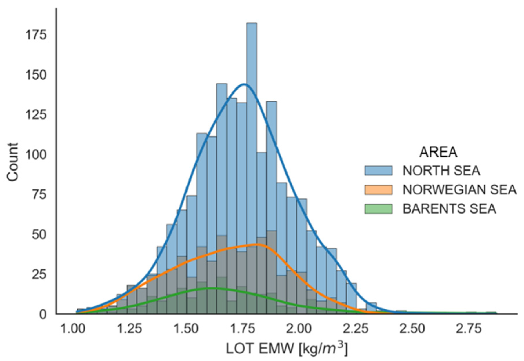
This study used geospatial information (the water depth, spatial coordinates, and the measured depths) as input features of the machine learning models to predict the leak-off pressures. The database analyzed comprised 1943 data points from the North Sea, 708 from the Norwegian Sea, and 268 from the Barents Sea. The data were from around 1800 wells and some wells had several data points if the well tests were performed in the different depths. Statistical information of the leak-off pressure values are summarized in Table 1. The data showed that the mean and standard deviation (SD) of leak-off pressure on the Norwegian Continental Shelf was 1.72 and 0.24 g/cm3, respectively. Comparing the statistics of each geographical area (Figure 2), the Barents Sea showed more scatter in the leak-off pressure (i.e., SD = 0.29) than the other two geographical areas (SD = 0.23 and 0.24).
Table 2 summarizes the statistics of the geospatial information in the three geographical areas: measured depth in mbsl (meters below sea level), water depth in m, latitude in ° and longitude in °. The LOP-values as a function of the geospatial parameters can be found in Figure 3. In the North Sea, the top of the petroleum reservoirs is often between 1500 and 3000 m below sea level. The LOP tests are usually conducted near the reservoir, with the casing shoe located at the caprock of reservoirs. The mean depth was shallower for the Barents Sea. The LOP data showed more scatter than the other two areas (the green outlier dots on Figure 3). The scatter may be related to the glacier erosion and uplift processes, which resulted in overconsolidation in the Barents Sea over the last few millions of years [14].
3. Machine Learning Algorithms
In this study, three machine learning models to predict the LOP were compared: deep neural network (DNN), random forest (RF), and support vector machine (SVM). The analyses were carried out in the Python programming environment with the machine learning package of Scikit-learn [15] for the RF and SVM model and the Keras [16] with TensorFlow backbone [17] for the DNN model.
3.1. Deep Neural Network
Deep neural networks (DNN) are a member of the deep learning family, which enables the formulation of strong regressor or classifier models. The main parts of the structure of a DNN include activation functions, the number and type of hidden layers and nodes, optimization algorithm, and loss function [18]. The rectified linear unit (ReLU) has been shown to enhance efficiency of the optimization [19], and therefore was adopted for the input and hidden layers. The activation function for the output layer was determined through optimization between ReLU and a linear unit. To avoid overfitting that could occur in fully connected NN architectures, some connections between neurons were randomly ignored using a drop-out technique. Learning rate and the dropout percentage were also optimized to avoid overfitting.
3.2. Random Forest (RF)
The random forest (RF) algorithm is an “ensemble” machine learning method for classification and regression. It consists of the construction of multiple decision trees [20]. The RF algorithm generates uncorrelated decision trees that operate together. The RF algorithm, with its ensemble of random decision trees, forms a forest to develop a more accurate prediction. Each tree is grown based on a re-sampling (bootstrap aggregating) technique. A classification and regression procedure is established through a random group of variables selected at each tree node. To ensure reliable predictions, at least two conditions should be verified: the selected variables should have some predictive ability; the different decision tree models need to be uncorrelated [21].
3.3. Support Vector Machine
The support vector machine (SVM) algorithm is a nonlinear regression forecasting method [22]. SVM models map data into a high-dimensional feature space through a non-linear transformation and then does linear regression within that space [23]. Particle swarm optimization (PSO) is applied to search for the optimal parameters of the SVM model. Inspired from the feeding behavior of a bird flock, the PSO is used for solving optimization problems [24], where each particle in the algorithm is regarded as a potential solution to the optimization problem. A fitness function is defined to search for the optimal solution in the entire solution space.
3.4. Performance Indicators for Machine Learning (ML) Models
To measure and compare the performance of the ML models for predicting the leak-off pressure, two performance indicators were adopted in this study: the root mean square error (RMSE) and the coefficient of determination R2. Lower RMSE values (with minimum of 0) and a higher R2-value (with maximum of 1) reflect good accuracy.
3.5. Hyperparameter Search Algorithms
The performance of machine learning algorithms can depend on the selected hyperparameters that control the learning process (e.g., number of hidden layers in a neural network, number of leaves in a tree-based model, etc.) [12]. To find an optimal set of hyperparameters resulting in the best performance, this study tested three algorithms: a grid search, a random search, and a Bayesian search algorithm. Each method seeks to find the set of parameters that give the highest score of the mean k-fold cross-validation. The k-fold cross-validation splits the train dataset into k subsets and trains the model using k-1 subsets and validates the trained model with the remaining k subset. This training and validation process is repeated k times by changing the subsets used for the training and testing. The mean validation score of each score is the final performance indicator.
The grid search algorithm [25] checks all different combinations of hyperparameters and finds the combination that results in the highest averaged validation score. It is straightforward and robust since it examines all possible combinations, but it is also very time-consuming. The random search algorithm [26] generates a random combination of hyperparameters and searches for the hyperparameter resulting in the best performance. The random search can be more efficient than the grid search if the random sets are well distributed in the parameter space. However, the accuracy can depend on the number of random trials. The Bayesian search algorithm [27] can efficiently optimize hyperparameters by building and updating a probability of hypothetical model of the real objective function that can sometimes be non-linear, non-convex, and implicit. It builds a surrogate probability model of the objective function. Through iteration, the algorithm selects the most promising hyperparameter(s) with an acquisition function based on the performance of the best performed surrogate model and updates it. The gaussian processes and the expected improvement were used as the surrogate model and the acquisition function for the Bayesian optimization algorithm, respectively. Other hyper parameters were set as the default value of the Scikit-optimize model [28].
4. Results of Analyses
4.1. Correlation Analysis of Leak-Off Pressure (LOP) Data
Correlation analysis and feature selection is an important step of the data pre-processing. Table 3 summarizes the Pearson correlation coefficients r and p-values between the leak-off pressure and the geospatial parameters. In this study, p-value was used to examine whether two variables were correlated, and the r-value was used to quantify the correlation strength between two variables. The p-value used in this study was used to evaluate how well the null hypothesis, which assumes that the correlation between two variables occurred by chance, can be rejected. If the p-value is high, it supports the null hypothesis and indicates that the two variables are likely to have no correlation and occurred by chance. However, a low p-value means that the null hypothesis can be rejected and there may be a correlation between two variables. When the significance threshold of 0.05 is applied to the p-value, the tested geospatial information seems to have statistically meaningful correlation with LOP in general. However, the latitude of the Barents Sea and the longitude of the North Sea showed high p-values (0.598 and 0.723, respectively) and indicates that there is no statistically meaningful correlation to the LOPs. Using the correlation classification in Table 4, the strength of the correlations was tested. The LOP in the North Sea only showed moderate correlation with measured depth (r of 0.64). For the Norwegian Sea, the LOP showed moderate correlation with measured depth (r of 0.58) and water depth (r of −0.42). For the Barents Sea, the LOP showed low correlation with measured depth (r of 0.25) and water depth (r of −0.22). The very low correlation coefficients for latitude and longitude indicate that these parameters may have a minor effect on the LOP.
4.2. Pre-Processed Data
This study used 80% of the dataset for training and the 20% of the dataset to test the ML models. When the data were split, the proportion of the original dataset (i.e., North Sea:Norwegian Sea:Barents Sea~19:7:3) was kept similar for the training and testing datasets. Figure 4 shows the histograms of the probabilistic density of the training and testing datasets. The training dataset was split into five subsets, and four of the subsets were used to train the model and the fifth one was used to validate the model. This was done iteratively, which is known as a 5-fold cross-validation, and was used to avoid overfitting. The training and testing datasets were then normalized using feature scaling to bring them into the same order of magnitude of differences between different measurements. Two types of feature scaling were used. The “standardization” approach transformed the data to zero mean and unit variance, and the “min-max normalization” scaled the data to a range between 0 to 1. The probabilistic densities of the unscaled and the two scaled datasets are shown in Figure 5. Figure 5 shows that without scaling, the values of LOP varied by two to three orders of magnitude. For example, the water depth and the measured depth range were 51–1721 m and 169–6619 m, respectively. Latitude and longitude (in °) varied over a much smaller range (62–74° and 1–31°). The normalization results in a much narrower range of values, which are easier to work with.
4.3. Accuracy and Calculation Time for Three Hyperparameter Optimization Methods
The hyperparameter optimization algorithms were tested to compare performance. The comparison study used RF algorithms as reference ML algorithms. Seven hyperparameters were optimized: the number of trees in the forest (i.e., n_estimator), the number of features to consider when looking for the best split (i.e., max_features), the maximum depth of the tree (i.e., max_depth), the minimum number of samples required to split an internal node (i.e., min_samples_split), the minimum number of samples required to be at a leaf node (i.e., min_samples_leaf), the Boolean data related to a reuse of the previous solution for the “ensemble” (i.e., warm_start), and the Boolean data on whether bootstrap samples are used when building trees (i.e., bootstrap). The training datasets were normalized with the min-max normalization technique.
Figure 6 presents the following results: the highest mean validation score, which is an index describing model accuracy, increases with number of iterations and time. The validation score is calculated from the average of k-folds cross validation scores. The best validation score of the Bayesian search appears to increase gradually, whereas the grid search takes a much longer time. If one compares the accuracy and optimization time of the three algorithms in Table 5, the test scores are similar, with an R2 coefficient close to 0.57. The test scores can be lower than the validation scores, as illustrated in Figure 6. The grid search algorithm took a longer optimization time because it searches among every possible combination of hyperparameters.
To investigate the efficiency of the optimization, the values for seven hyperparameters optimized by the Bayesian search algorithm were compared with the sample spaces during optimization (Figure 7). Theoretically, the sample spaces for both the grid search and random search should be uniform. The generated sample spaces for those two algorithms look rather uniform in Figure 7. Non-uniform sample spaces for some parameters are related to non-uniform search spaces (e.g., search space of the n-estimator for the grid search is [100,200,400,600,800,1000] but other algorithms have the space from 1 to 1000).
The Bayesian search generated more samples close to the optimal hyperparameter because it suggests a new set of the most promising hyperparameters based on the previous observation. This results in the Bayesian search becoming more effective as the number of iterations increases.
4.4. Accuracy and Calculation Time for Three Machine Learning Algorithms
The three machine learning algorithms were used to model the datasets. The input data were normalized with the min-max normalization. The hyper parameters of three ML models (e.g., the number of layers and the number of nodes for each layer for the DNN model, the maximum depth of layers and the number of nodes for each layer for the DNN model, the maximum depth of the tree, and the number of trees in the forest for RF model) were optimized with the Bayesian search algorithm. The search range and optimal value of the hyperparameters for the three ML algorithms are summarized in Table 6. The machine learning model performance was compared with the results of multivariate linear regression.
The calculated test score and required train time are summarized in Table 7. The three machine learning algorithms showed higher test scores (R2 coefficient of 0.53–0.57) than the multivariate linear regression (R2 coefficient of 0.42). The random forest model resulted in a higher test score (0.57) than the other two machine learning models. In terms of efficiency, the random forest regression resulted in a higher mean validation score and shorter optimization times than the deep neural network model, as shown in Figure 8.
The model inputs were also normalized by the standardization approach instead of the min-max normalization. The test scores remained quite similar (Figure 9). However, when the inputs were not scaled, the support vector machine and neural network regression algorithms had lower scores than the linear regression. The random forest regression model had similar scores, regardless of data scaling.
4.5. Effect of Data Grouping on the Machine Learning Prediction
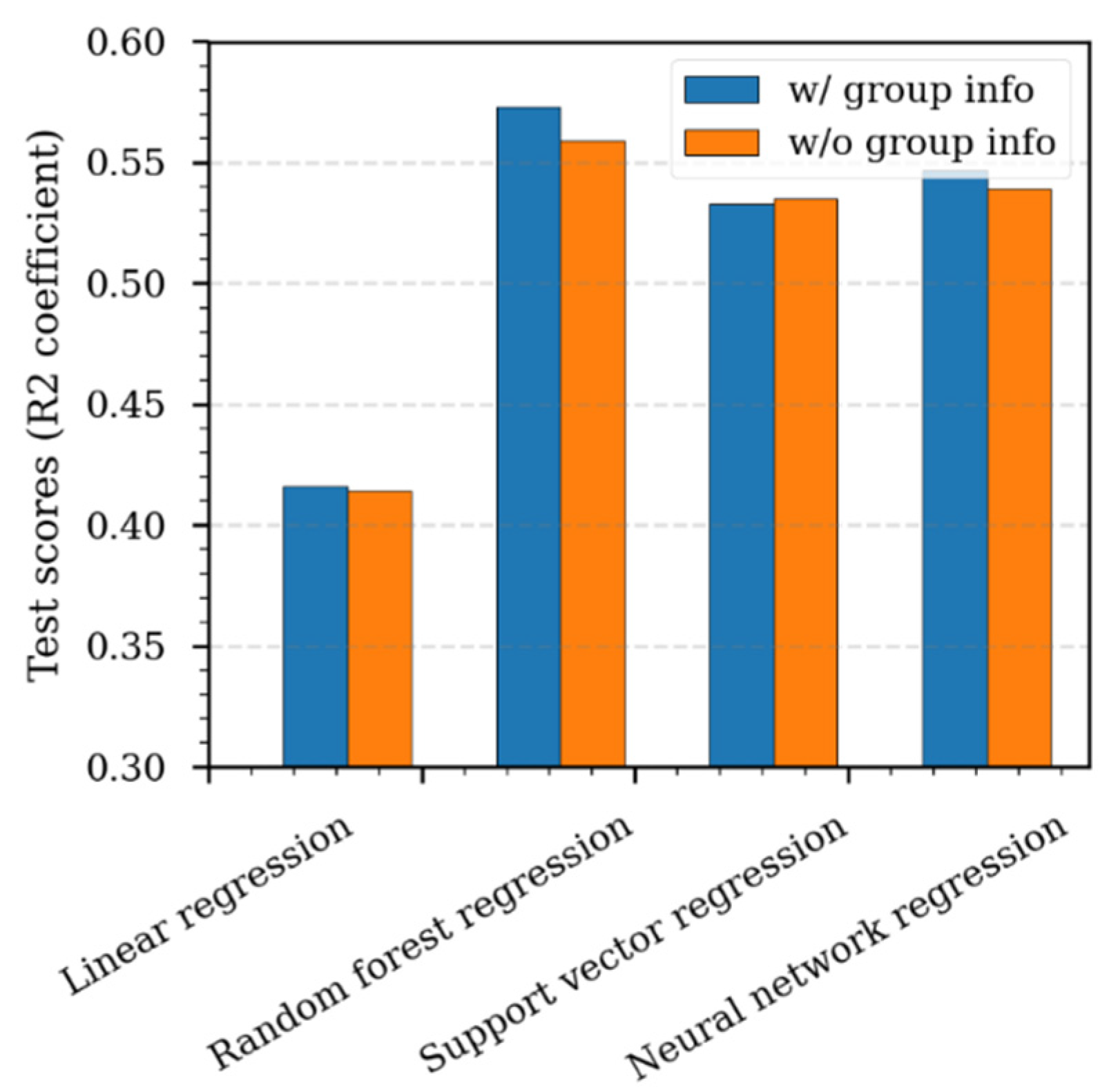
The effect of including categorized geographical area information on the machine learning prediction of LOP was tested. A case without any geographical area information, in other words all data placed into one single set, was analyzed with the random forest regression algorithm. The data were scaled with the min-max normalization. Figure 10 compares the test scores for the RF analyses with and without the geographical area information. The analyses show that the case including the geographical information had essentially the same test scores as the case without the geographical area information. The differences were also negligible for the other two machine learning algorithms. The three machine learning models showed better performance than the multivariate linear regression.
The trained RF regression model was tested for each geographical area separately. Figure 11 shows the resulting test scores for the predicted LOP-value. The test score was highest for the Norwegian Sea (0.75), and 0.60 for the North Sea. For the Barents Sea, with only 268 data points, the test score was unsatisfactorily low (−0.09). Figure 12 compares the measured and predicted LOP-values using the RF regression model. There was good agreement for the North Sea and the Norwegian Sea. The predicted Barents Sea LOP values, however, had only a very weak or no correlation with the measured values.
5. Discussion
5.1. Performance of the Three Machine Learning Algorithms
Among the three ML algorithms tested, the RF algorithm gave the most promising results. The performance of the RF model was not dependent of scaling because it is a tree-based algorithm that does not require feature scaling [30]. The RF model gave better results than the deep neural network (DNN), although DNNs have performed better than other machine learning algorithms for many industrial applications (e.g., image processing, language recognition) [31,32]. However, this was not the case for the LOP in offshore formations. This may be due to the deep network showing poorer performance for lower quantities of data: larger quantities of data would be needed for a good performance of a more complex deep neural network. Figure 13 investigates the optimized neural network model in the sample space of the Bayesian search. The data showed that there are more samples on the shallower (n_layer < 5) and wider neural networks (number of node in hidden layer > 500) than in the deeper networks. The second largest of the sampled hidden layers (n_layer in Figure 13) is a single layer only, which is recognized as a shallow neural network. Figure 13 suggests that a shallower neural network may perform better than a deeper neural network when there are a limited number of data points (<3000 data points). It is well known that deep neural networks can perform better than traditional algorithms when the number of data is large enough, which is known as “big data” [33]. However, this study indicates that traditional machine learning algorithms, especially RF algorithms, could well be a preferable solution if the data have a limited amount and is geospatially scattered like typical geotechnical and geological borehole data. Furthermore, other advanced ML algorithms that can combine the advantages of algorithms (e.g., gradient boosting with random forest, kriging combined ML, etc.) can be a useful way to enhance predictions.
5.2. Correlation between LOP and Geospatial Information
The best test score of optimized algorithms, in this case, the random forest regression model optimized by the Bayesian search, was about 0.57, which was not higher than the highest Pearson correlation coefficient r (i.e., 0.57). Interestingly, the LOP prediction for the Norwegian Sea had the highest test score among the geographical areas although (1) the number of data points (700) was smaller than the dataset for the North Sea (1943 data points) and (2) its highest correlation coefficient (0.58 for the measured depth) was lower than that for the North Sea (0.64). The one difference is that the Norwegian Sea data had moderate correlation with two parameters, the measured depth and the water depth, while the North Sea data had moderate correlation with only one variable, the measured depth. This may indicate that selecting the appropriate input parameters may be more important than the number of data points. The poor prediction for the smaller Barents Sea dataset with different geological characteristics may also support this hypothesis. An appropriate selection and filtering of key parameters and elimination of irrelevant parameters can be as important as the quantity of data. Other studies by Micheletti et al. [34] have highlighted the importance of feature correction and input selection for improved accuracy of machine learning models. In addition to the tested ML algorithms, kriging methods could be better predictors for the geospatial databases that have weak correlation [35]. However, these are still hypothetical ideas from limited cases that need to be validated by further systematic studies.
An interesting observation from this study is the poor correlation of LOP with depth for the Barents Sea dataset. This observation is believed to reflect the complex geological history of the Barents Sea. Much more significant erosion and uplift of the Barents Sea compared to the North Sea and Norwegian Sea has resulted in a very different stress history for the Barents Sea region. Large uncertainty has been observed in stress measurements in the Barents Sea with strong local variations, both horizontally and vertically [36], and a weakly defined stress regime. In the North Sea and the Norwegian Sea, the stress conditions and geological processes are simpler and it is possible to define a normal stress regime within the sedimentary basin [37]. This suggests that geological parameters such as tectonic stress regime and uplift and overconsolidation, if included in the analysis, have the potential to improve the prediction. Other parameters like the lithological variations for the LOP measurements and distance to geological structures with local stress alterations (e.g., faults, might also be relevant for inclusion in further studies of ML prediction capabilities).
6. Conclusions
In this paper, the leak-off pressures in deep formations offshore Norway were predicted using weakly correlated geospatial input and machine learning algorithms. The geo-referenced dataset comprised about 3000 leak-off pressure tests from 1800 exploration wells collected from the Norwegian Petroleum Directorate (NPD) “fact pages”. Three machine learning algorithms and three hyperparameter optimization algorithms were tested. The main findings from the study are:
- The Bayesian search algorithm was able to optimize hyperparameters more efficiently than the grid search and random search algorithms.
- The three machine learning algorithms (random forest, support vector machine, deep neural network) showed higher predictive scores than the multivariate linear regression. However, if the inputs were not scaled, the support vector machine and the neural network regression algorithms resulted in poorer scores than the multivariate linear regression.
- When the geographical area information (i.e., North Sea, Norwegian Sea, and Barents Sea) was taken separately in the machine learning analysis, the models performed only slightly better than the models considering all data from the three geographical areas together.
- However, even well-optimized models do not result in meaningfully higher test scores than its highest correlation coefficient or the score of linear regression. This could be related to the small number of data points (3000 or less) and the weak correlation between the LOP and the input (i.e., geospatial) parameters.
- For geomechanics and geotechnics applications, where there are limited numbers of data (e.g., less than 10,000 data points), this study clearly shows that the random forest regression algorithm with Bayesian parameter optimization provides a promising performance in terms of accuracy and short calculation times. However, test scores that are not meaningfully higher than moderate correlation coefficients may suggest that accurate predictions can depend more on the number of well-correlated parameters available than the use of fancy ML algorithms and advanced optimization algorithms.
Author Contributions
Conceptualization, J.C.C., E.S., and Z.L.; Methodology, J.C.C. and Z.L.; Software, J.C.C.; Data analysis, J.C.C., Z.L., S.L., and E.S.; Writing: original draft preparation: J.C.C., Z.L., and S.L.; Writing: review and editing, S.L. and E.S.; Funding, E.S. All authors have read and agreed to the published version of the manuscript.
Funding
The funding for the research was supported by the Research Council of Norway for the NCCS (Norwegian CCS Research Center) (Grant 257579/E20), one of the Norwegian Centers for Environment-friendly Energy Research (FME), and the OASIS (Overburden Analysis and Seal Integrity Study for CO2 Sequestration in the North Sea) project (NFR-CLIMIT project #280472).
Acknowledgments
The authors acknowledge the following partners supporting this research: Aker Solutions, ANSALDO Energia, CoorsTek Membrane Sciences, EMGS, Equinor, Gassco, KROHNE, Larvik Shipping, Norcem, Norwegian Oil and Gas, Quad Geometrics, Shell, TOTAL, and The Research Council of Norway. NGI is grateful to the Norwegian Petroleum Directorate for providing the databases and making this work possible.
Conflicts of Interest
The authors declare no conflict of interest.
References
- Zhang, J.; Yin, S.-X. Fracture Gradient Prediction: An Overview and an Improved Method. Pet. Sci. 2017, 14, 720–730. [Google Scholar] [CrossRef] [Green Version]
- Eaton, B.A. Fracture Gradient Prediction and Its Application in Oilfield Operations. J. Pet. Technol. 1969, 21, 1353–1360. [Google Scholar] [CrossRef]
- Hubbert, M.K.; Willis, D.G. Mechanics of Hydraulic Fracturing. Trans. AIME 1957, 210, 153–168. [Google Scholar] [CrossRef]
- Matthews, W.R.; Kelly, J. How to Predict Formation Pressure and Fracture Gradient. Oil Gas J. 1967, 65, 92–1066. [Google Scholar]
- Breckels, I.M.; van Eekelen, H.A.M. Relationship between Horizontal Stress and Depth in Sedimentary Basins. J. Pet. Technol. 1982, 34, 2191–2199. [Google Scholar] [CrossRef]
- Andrews, J.S.; de Lesquen, C. Stress Determination from Logs. Why the Simple Uniaxial Strain Model Is Physically Flawed but Still Gives Relatively Good Matches to High Quality Stress Measurements Performed on Several Fields Offshore Norway; 53rd U.S. Rock Mechanics/Geomechanics Symposium: New York, NY, USA, June 2019. [Google Scholar]
- Wrona, T.; Pan, I.; Gawthorpe, R.L.; Fossen, H. Seismic Facies Analysis Using Machine LearningMachine-Learning-Based Facies Analysis. Geophysics 2018, 83, O83–O95. [Google Scholar] [CrossRef]
- Jia, Y.; Ma, J. What Can Machine Learning Do for Seismic Data Processing? An Interpolation Application. Geophysics 2017, 82, V163–V177. [Google Scholar] [CrossRef]
- Yin, Z.; Jin, Y.; Liu, Z. Practice of Artificial Intelligence in Geotechnical Engineering. J. Zhejiang Univ. Sci. A 2020, 21, 407–411. [Google Scholar] [CrossRef]
- Factpages—NPD. Available online: https://factpages.npd.no/ (accessed on 1 December 2020).
- Choi, J.C.; Skurtveit, E.; Grande, L. Deep Neural Network Based Prediction of Leak-Off Pressure in Offshore Norway. In Proceedings of the Offshore Technology Conference, Houston, TX, USA, 26 April 2019. [Google Scholar]
- Bergstra, J.; Bardenet, R.; Bengio, Y.; Kégl, B. Algorithms for Hyper-Parameter Optimization. Adv. Neural Inf. Process. Syst. 2011, 24, 2546–2554. [Google Scholar]
- Beautiful Soup Documentation—Beautiful Soup 4.4.0 Documentation. Available online: https://beautiful-soup-4.readthedocs.io/en/latest/# (accessed on 1 December 2020).
- Fejerskov, M.; Lindholm, C. Crustal Stress in and around Norway: An Evaluation of Stress-Generating Mechanisms. Geol. Soc. Lond. Spec. Publ. 2000, 167, 451–467. [Google Scholar] [CrossRef]
- Pedregosa, F.; Varoquaux, G.; Gramfort, A.; Michel, V.; Thirion, B.; Grisel, O.; Blondel, M.; Prettenhofer, P.; Weiss, R.; Dubourg, V.; et al. Scikit-Learn: Machine Learning in Python. J. Mach. Learn. Res. 2011, 12, 2825–2830. [Google Scholar]
- Chollet, F. Keras: Deep Learning Library for Theano and Tensorflow. 2015. Available online: https://Keras.Io (accessed on 15 June 2019).
- Abadi, M.; Barham, P.; Chen, J.; Chen, Z.; Davis, A.; Dean, J.; Devin, M.; Ghemawat, S.; Irving, G.; Isard, M.; et al. TensorFlow: A System for Large-Scale Machine Learning; USENIX: Savannah, GA, USA, 2016; pp. 265–283. [Google Scholar]
- Bengio, Y. Learning Deep Architectures for AI; Now Publishers Inc.: Delft, The Netherlands, 2009; Volume 2, pp. 1–127. [Google Scholar] [CrossRef]
- Glorot, X.; Bordes, A.; Bengio, Y. Deep Sparse Rectifier Neural Networks. In Proceedings of the Fourteenth International Conference on Artificial Intelligence and Statistics, Fort Lauderdale, FL, USA, 11–13 April 2011; Volume 15, pp. 315–323. [Google Scholar]
- Breiman, L. Random Forests. Mach. Learn. 2001, 45, 5–32. [Google Scholar] [CrossRef] [Green Version]
- Liu, Z.; Gilbert, G.; Cepeda, J.M.; Lysdahl, A.O.K.; Piciullo, L.; Hefre, H.; Lacasse, S. Modelling of Shallow Landslides with Machine Learning Algorithms. Geosci. Front. 2021, 12, 385–393. [Google Scholar] [CrossRef]
- Cortes, C.; Vapnik, V. Support-Vector Networks. Mach. Learn. 1995, 20, 273–297. [Google Scholar] [CrossRef]
- Smola, A.J.; Schölkopf, B. A Tutorial on Support Vector Regression. Stat. Comput. 2004, 14, 199–222. [Google Scholar] [CrossRef] [Green Version]
- Eberhart, R.; Kennedy, J. A New Optimizer Using Particle Swarm Theory. In Proceedings of the MHS’95, the Sixth International Symposium on Micro Machine and Human Science, Nagoya, Japan, 4–6 October 1995; pp. 39–43. [Google Scholar]
- Chicco, D. Ten Quick Tips for Machine Learning in Computational Biology. BioData Min. 2017, 10. [Google Scholar] [CrossRef] [PubMed]
- Bergstra, J.; Bengio, Y. Random Search for Hyper-Parameter Optimization. J. Mach. Learn. Res. 2012, 13, 281–305. [Google Scholar]
- Snoek, J.; Larochelle, H.; Adams, R.P. Practical Bayesian Optimization of Machine Learning Algorithms. arXiv 2012, arXiv:12062944. [Google Scholar]
- Head, T.; MechCoder, G.L.; Shcherbatyi, I. Scikit-Optimize/Scikit-Optimize: V0.5.2; Zenodo: 2018. Available online: http://0-doi-org.brum.beds.ac.uk/10.5281/zenodo.1207017 (accessed on 18 April 2021).
- Hinkle, D.E.; Wiersma, W.; Jurs, S.G. Applied Statistics for the Behavioral Sciences; Houghton Mifflin: Boston, MA, USA, 2003; ISBN 978-0-618-12405-3. [Google Scholar]
- Liaw, A.; Wiener, M. Classification and Regression by RandomForest. R News 2001, 2–3, 18–22. [Google Scholar]
- Brown, T.B.; Mann, B.; Ryder, N.; Subbiah, M.; Kaplan, J.; Dhariwal, P.; Neelakantan, A.; Shyam, P.; Sastry, G.; Askell, A.; et al. Language Models Are Few-Shot Learners. arXiv 2020, arXiv:200514165. [Google Scholar]
- Szegedy, C.; Liu, W.; Jia, Y.; Sermanet, P.; Reed, S.; Anguelov, D.; Erhan, D.; Vanhoucke, V.; Rabinovich, A. Going Deeper with Convolutions. In Proceedings of the 2015 IEEE Conference on Computer Vision and Pattern Recognition (CVPR), Boston, MA, USA, 7–12 June 2015; pp. 1–9. [Google Scholar]
- Ng, A. CS229 Course Notes: Deep Learning; Stanford University: Stanford, CA, USA, 2018. [Google Scholar]
- Micheletti, N.; Foresti, L.; Robert, S.; Leuenberger, M.; Pedrazzini, A.; Jaboyedoff, M.; Kanevski, M. Machine Learning Feature Selection Methods for Landslide Susceptibility Mapping. Math. Geosci. 2014, 46, 33–57. [Google Scholar] [CrossRef] [Green Version]
- Veronesi, F.; Schillaci, C. Comparison between Geostatistical and Machine Learning Models as Predictors of Topsoil Organic Carbon with a Focus on Local Uncertainty Estimation. Ecol. Indic. 2019, 101, 1032–1044. [Google Scholar] [CrossRef]
- Chiaramonte, L.; White, J.A.; Trainor-Guitton, W. Probabilistic Geomechanical Analysis of Compartmentalization at the Snøhvit CO2 Sequestration Project. J. Geophys. Res. Solid Earth 2015, 120, 1195–1209. [Google Scholar] [CrossRef] [Green Version]
- Andrews, J.; Fintland, T.G.; Helstrup, O.A.; Horsrud, P.; Raaen, A.M. Use of Unique Database of Good Quality Stress Data to Investigate Theories of Fracture Initiation, Fracture Propagation and the Stress State in the Subsurface; American Rock Mechanics Association: Houston, TX, USA, 2016. [Google Scholar]
Figure 1.
Leak-off pressure values collected from the Norwegian Petroleum Directorate (NPD) database (left) and geographical location of the three datasets (right).
Figure 1.
Leak-off pressure values collected from the Norwegian Petroleum Directorate (NPD) database (left) and geographical location of the three datasets (right).

Figure 2.
Histograms of leak-off pressures for the three geographical areas.

Figure 3.
Joint scatter plots of leak-off pressure and geospatial information.

Figure 4.
Probabilistic density histograms of training and testing datasets of input variables (left to right): (a) depth of measurements (meter below sea level); (b) water depth; (c) longitude; (d) latitude; and (e) geographical area.
Figure 4.
Probabilistic density histograms of training and testing datasets of input variables (left to right): (a) depth of measurements (meter below sea level); (b) water depth; (c) longitude; (d) latitude; and (e) geographical area.

Figure 5.
Non-scaled training dataset (left) and scaled training dataset with standardization (center) and min-max normalization (right); the units of the horizontal scale can be found in the legend.
Figure 5.
Non-scaled training dataset (left) and scaled training dataset with standardization (center) and min-max normalization (right); the units of the horizontal scale can be found in the legend.

Figure 6.
Mean validation score and fitting time for three hyperparameter optimization algorithms.

Figure 7.
Probabilistic density histograms of sampled hyperparameter spaces with three algorithms compared with the hyperparameters optimized by the Bayesian search algorithm.
Figure 7.
Probabilistic density histograms of sampled hyperparameter spaces with three algorithms compared with the hyperparameters optimized by the Bayesian search algorithm.

Figure 8.
Mean validation score and required fitting time for three machine learning algorithms.

Figure 9.
Effect of data scaling on the test score of three machine learning algorithms.

Figure 10.
Effect of data grouping on the prediction performance of three machine learning algorithms.
Figure 10.
Effect of data grouping on the prediction performance of three machine learning algorithms.

Figure 11.
Test scores for each of the three geographical areas using the random forest (RF) machine learning algorithm.
Figure 11.
Test scores for each of the three geographical areas using the random forest (RF) machine learning algorithm.

Figure 12.
Scatter plots of the measured and predicted leak-off pressures of test samples using the RF model in each geographical area.
Figure 12.
Scatter plots of the measured and predicted leak-off pressures of test samples using the RF model in each geographical area.

Figure 13.
Probabilistic density histograms of sample space for neural network regression with Bayesian search compared with the estimated optimal hyperparameter.
Figure 13.
Probabilistic density histograms of sample space for neural network regression with Bayesian search compared with the estimated optimal hyperparameter.


Table 1.
Statistics of leak-off pressures in analysis.
| Geographical Area | Number of Data Points | LOP EMW a [g/cm3] | ||||||
|---|---|---|---|---|---|---|---|---|
| Mean | SD b | Min c | 25% d | 50% e | 75% f | Max g | ||
| North Sea | 1943 | 1.74 | 0.23 | 1.02 | 1.59 | 1.74 | 1.89 | 2.53 |
| Norwegian Sea | 708 | 1.69 | 0.24 | 1.02 | 1.51 | 1.70 | 1.87 | 2.36 |
| Barents Sea | 268 | 1.65 | 0.29 | 1.03 | 1.47 | 1.62 | 1.80 | 2.87 |
| All NCS h | 2919 | 1.72 | 0.24 | 1.02 | 1.57 | 1.73 | 1.88 | 2.87 |
a Equivalent mud weight, b Standard deviation, c Minimum LOP in measured data, d–f 25, 50, 75 percentile, g Maximum LOP in measured data, h Norwegian Continental Shelf.
Table 2.
Statistics of geospatial information for leak-off pressures in the analyses.
| Geographical Area | TVD MSLa [m] | Water Depth [m] | Latitude [°] | Longitude [°] | ||||
|---|---|---|---|---|---|---|---|---|
| Mean | SD | Mean | SD | Mean | SD | Mean | SD | |
| North Sea | 1905.7 | 1147.9 | 162.7 | 105.5 | 59.46 | 1.78 | 2.67 | 0.67 |
| Norwegian Sea | 2054.8 | 1123.6 | 420.9 | 313.1 | 65.08 | 0.99 | 6.96 | 1.36 |
| Barents Sea | 1417.2 | 845.1 | 333.3 | 131.2 | 71.94 | 0.65 | 21.95 | 2.86 |
| All NCS | 1901.7 | 1122.9 | 238.6 | 211.3 | 61.90 | 4.17 | 5.37 | 5.52 |
a True vertical depth below mean sea level.
Table 3.
Pearson correlation coefficients r and the p-value between leak-off pressure (LOP) and geospatial information.
Table 3.
Pearson correlation coefficients r and the p-value between leak-off pressure (LOP) and geospatial information.
| LOP Geographical Location | Depth of LOP Measurement | Water Depth | Latitude | Longitude | ||||
|---|---|---|---|---|---|---|---|---|
| r | p-Value | r | p-Value | r | p-Value | r | p-Value | |
| North Sea | 0.64 | <0.001 | −0.17 | <0.001 | −0.23 | <0.001 | −0.01 | 0.723 |
| Norwegian Sea | 0.58 | <0.001 | −0.42 | <0.001 | −0.10 | 0.028 | 0.15 | <0.001 |
| Barents Sea | 0.25 | 0.004 | −0.22 | 0.001 | −0.07 | 0.598 | 0.16 | 0.004 |
| All NCS | 0.57 | <0.001 | −0.29 | <0.001 | −0.18 | <0.001 | −0.08 | <0.001 |
Table 4.
Correlation classification used for this study. Modified from Hinkle et al. [29].
Table 4.
Correlation classification used for this study. Modified from Hinkle et al. [29].
| Absolute Correlation Coefficient r | Interpretation |
|---|---|
| 0.9–1.0 | Very strong |
| 0.7–0.9 | Strong |
| 0.4–0.7 | Moderate |
| 0.2–0.4 | Weak |
| 0.0–0.2 | Negligible |
Table 5.
Accuracy and calculation times for three hyperparameter optimization methods.
| Performance Parameter | Grid Search | Random Search | Bayesian Search | |
|---|---|---|---|---|
| Accuracy of test dataset | RMSE a | 0.158 | 0.157 | 0.158 |
| R2 b | 0.567 | 0.572 | 0.570 | |
| Accuracy of train dataset | RMSE | 0.055 | 0.079 | 0.055 |
| R2 | 0.945 | 0.889 | 0.946 | |
| Total calculation time [s] | 10,795.5 | 733.2 | 1251.9 | |
| Number of iterations | 4536 | 100 | 100 | |
| Calculation time per iteration [s] | 2.4 | 7.3 | 12.5 | |
a. root-mean-square error, b. coefficient of determination.
Table 6.
Search range and optimized hyperparameters for the tested ML algorithms.
| ML Algorithms | Hyperparameters | Search Range | Optimized Value |
|---|---|---|---|
| RF | max_depth | 1–100 | 63 |
| max_features | [‘auto’, ‘sqrt’, ‘log2’] | sqrt | |
| min_samples_leaf | 1–5 | 1 | |
| min_samples_split | 2–10 | 2 | |
| n_estimators | 1–1000 | 782 | |
| bootstrap | [True, False] | TRUE | |
| warm_start | [True, False] | True | |
| SVM | C | 1–1000 | 1 |
| gamma | 0.01–100 | 69.077 | |
| DNN | batch_size | 10–1000 | 345 |
| epochs | 100–1000 | 892 | |
| n_layer | 1–10 | 5 | |
| n_node_in_layer | 4–1024 | 958 | |
| drop_out_percent | 0–0.9 | 0.05 | |
| learning_rate | 0.0001–0.01 | 0.0008 | |
| activation_output | [Relu, Linear] | Relu |
Table 7.
Test scores and calculation times for three machine learning algorithms.
| Test Score | Multivariate Linear Regression | RF | SVM | DNN |
|---|---|---|---|---|
| RMSE | 0.184 | 0.157 | 0.164 | 0.162 |
| R2 | 0.416 | 0.573 | 0.534 | 0.547 |
| Calculation time [s] | <1 | 996 | 283 | 47,853 |
Publisher’s Note: MDPI stays neutral with regard to jurisdictional claims in published maps and institutional affiliations. |
© 2021 by the authors. Licensee MDPI, Basel, Switzerland. This article is an open access article distributed under the terms and conditions of the Creative Commons Attribution (CC BY) license (https://creativecommons.org/licenses/by/4.0/).
Share and Cite
MDPI and ACS Style
Choi, J.C.; Liu, Z.; Lacasse, S.; Skurtveit, E. Leak-Off Pressure Using Weakly Correlated Geospatial Information and Machine Learning Algorithms. Geosciences 2021, 11, 181. https://0-doi-org.brum.beds.ac.uk/10.3390/geosciences11040181
AMA Style
Choi JC, Liu Z, Lacasse S, Skurtveit E. Leak-Off Pressure Using Weakly Correlated Geospatial Information and Machine Learning Algorithms. Geosciences. 2021; 11(4):181. https://0-doi-org.brum.beds.ac.uk/10.3390/geosciences11040181
Chicago/Turabian StyleChoi, Jung Chan, Zhongqiang Liu, Suzanne Lacasse, and Elin Skurtveit. 2021. "Leak-Off Pressure Using Weakly Correlated Geospatial Information and Machine Learning Algorithms" Geosciences 11, no. 4: 181. https://0-doi-org.brum.beds.ac.uk/10.3390/geosciences11040181
Note that from the first issue of 2016, this journal uses article numbers instead of page numbers. See further details here.