Gaussian Transformation Methods for Spatial Data

Abstract

Data gaussianity is an important tool in spatial statistical modeling as well as in experimental data analysis. Usually field and experimental observation data deviate significantly from the normal distribution. This work presents alternative methods for data transformation and revisits the applicability of a modified version of the well-known Box-Cox technique. The recently proposed method has the significant advantage of transforming negative sign (fluctuations) data in advance to positive sign ones. Fluctuations derived from data detrending cannot be transformed using common methods. Therefore, the Modified Box-Cox technique provides a reliable solution. The method was tested in average rainfall data and detrended rainfall data (fluctuations), in groundwater level data, in Total Organic Carbon wt% residuals and using random number generator simulating potential experimental results. It was found that the Modified Box-Cox technique competes successfully in data transformation. On the other hand, it improved significantly the normalization of negative sign data or fluctuations. The coding of the method is presented by means of a Graphical User Interface format in MATLAB environment for reproduction of the results and public access.

1. Introduction

Geostatistics in terms of kriging methodology is a scientific discipline with wide application field. In the area of water resources, it has been successfully applied to express the spatial variability of two very important hydro-geological variables such as groundwater and rainfall, e.g., [1,2,3]. A common problem with such observation data is the non-Gaussianity of them. A normal distribution is usually desirable in linear geostatistics [4]. If data are skewed the kriging estimator is affected. Data with important deviation from normality can be more suitable for geostatistical analysis after an appropriate transformation. While normality may not be strictly required, outliers and serious violations of skewness and kurtosis, can affect the variogram structure and the fitting process, and thus, the kriging results [5,6]. A gaussian distribution provides more stable variograms [7,8,9].

Ordinary kriging is applied very often for spatial analysis of variable sources of data and it is well-known to be optimal when the data have a multivariate normal distribution. Kriging represents variability only up to the second order moment (covariance). Data transformation then may be necessary to normalize the data distribution and reduce the effect of outliers, improving also the sample’s stationarity [7,10]. Thus, the estimation process is applied in the gaussian domain which allows to provide unbiased estimates at non-sampled locations before back-transforming to the original scale [10,11]. Re-transformation is a major limitation of such methods. Therefore, in this work, the proposed methodology assures the successful re-transformation to the original data scale. There is always the potential of application of a non-linear kriging method [12]. However, a successful data transformation to normal distribution and the application of a linear geostatistical method is a more straightforward solution in terms of methodological steps.

The proposed methodology is based on the well-known Box-Cox method, but can be applied on fluctuations as well. It has been successfully presented and applied on groundwater data in a previous work [13], but herein the complete framework of the method, its applicability to variable datasets and the code in terms of a MATLAB function is presented using a Graphical User Interface (GUI) for the parameters’ selection. The aim of this technical paper is the introduction of the method for general application on data analysis and modeling topics. A successful data transformation close to gaussian distribution is useful for different scientific disciplines to improve modeling accuracy [14,15,16,17].

2. Methodology

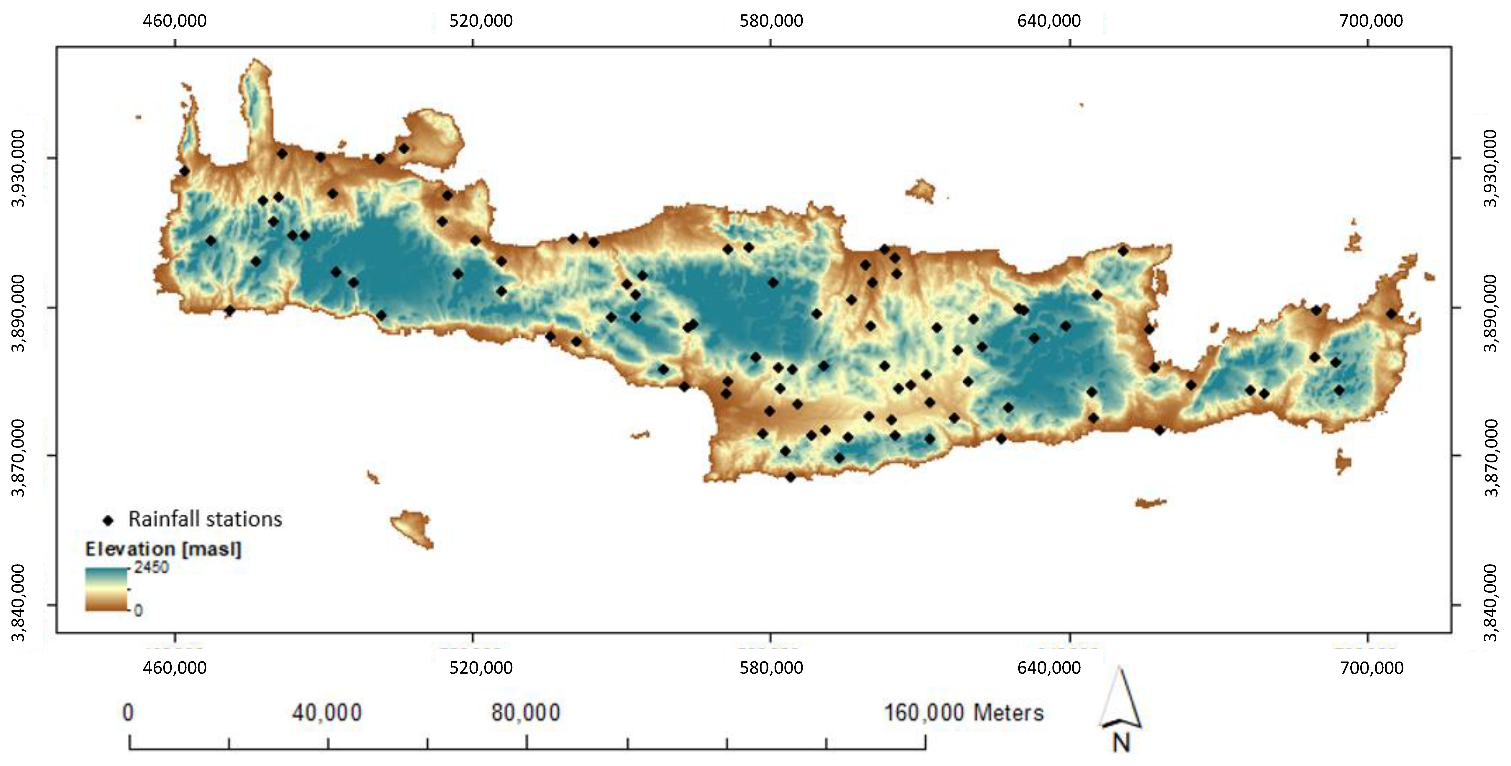
Three data sets were used to assess the credibility of the proposed method. The first one consisted of cumulative annual rainfall measurements processed from historical averages of 100 monitoring stations unevenly spatially distributed at the island of Crete, Greece (Figure 1). The dataset was processed for the purpose of this work, so specific details are presented. The range of rainfall values varies from 316.4 mm to 2015.23 mm with a standard deviation of 312.35 mm. Detrending of the data using the elevation of each station was also applied a priori in order to work with the fluctuations and test the method for negative sign values as well. It has to be noted that detrending of rainfall data with auxiliary correlated variables, i.e., elevation is a common practice in geostatistics to approximate non-stationarity of the data [18,19,20]. Herein the Pearson correlation coefficient is equal to 0.57 with a p-value of < 0.00001 meaning that the result is significant at p < 0.01. On the other hand, rainfall spatial representation depends on other physical factors as well, e.g., distance from the sea, exposure of the slopes, distribution (coordinates) of monitoring locations. Such information, if available, should be also considered in rainfall data detrending, to account for an integrated approach to approximate the rainfall spatial variability. In addition, the temporal scale and the time period of available data is another important factor that affects the dynamic spatial representation of rainfall distribution [21,22,23,24,25,26,27]. Depending on the case and time scale, appropriate detrending and data transformation should apply before geostatistical analysis with kriging.

The other two datasets consisted of groundwater level data in the area of Crete, Greece, available online by the Special Water Secretariat of Greece [28] and Total Organic Carbon wt% data from source rock samples available online from the United States Geological Survey (USGS) [29]. The first dataset includes values below sea level surface (negative sign), while the latter was also detrended and accounts for negative sign values analysis as well.

Well-known statistical metrics that certify data gaussianity are kurtosis ${\widehat{k}}_z$ and skewness ${\widehat{s}}_z$ coefficients (1), (2). The kurtosis of normal distribution is equal to 3 and the skewness equal to 0:

$${\widehat{k}}_z=\frac{\frac{1}{N}{\displaystyle \sum _{i=1}^N{\left(z_i-{\widehat{m}}_z\right)}^4}}{{\widehat{\sigma }}_z^4}$$

(1)

$${\widehat{s}}_z=\frac{\frac{1}{N}{\displaystyle \sum _{i=1}^N{\left(z_i-{\widehat{m}}_z\right)}^3}}{{\widehat{\sigma }}_z^3}$$

(2)

where $\mathbf{z}$ is the sample; $z_i$ is the sample variable i = 1…N; ${\widehat{m}}_z$ the sample mean; ${\widehat{\sigma }}_z$ is standard deviation and N is the number of observations.

The most well-known methods for gaussian data transformation and the corresponding advantages and disadvantages are presented in the

Table 1. Common transformation methods.

Method	Advantages	Disadvantages
Log	Right skewed data, log10(x) is especially good at handling higher order powers of 10	Zero values Negative values
Square Root	Right skewed data	Negative values
Square	Left skewed data	Negative values
Cube Root	Right skewed data Negative values	Not as effective at normalizing as log transform
1/x	Making small values bigger and big values smaller	Zero values Negative values

. The main limitation of these methodologies is their applicability to negative sign data. The cube root only can be applied to negative data but it does not provide, in principle, effective transformations [30].

Another technique that considers negative sign data transformation is the z-score transformation. However, in z-score, the transformed dataset is actually standardized with mean 0 and standard deviation 1, but retains the shape properties of the original dataset (same skewness and kurtosis). The aforementioned properties are an important reason for the application and development of non-linear techniques that could also process negative sign data [31].

A non-linear approach that has been widely used to transform environmental data close to gaussian distributions is the Box-Cox (BC) method [32]. The transformation function accounts for only positive data values and is defined in terms of the Equation (3).

$$y:=g_{BC}(z;k)=\{\begin{array}{ll}\frac{(z^k-1)}{k},& k\ne 0\\ \log (z),& k=0\end{array}$$

(3)

Given the vector of data observations ${\mathbf{z}}^T=(z_1,\dots ,z_N)$, the optimal value of the power exponent k, which leads to the best agreement of ${\mathbf{y}}^T=\left(g_k(z_1),\dots ,g_k(z_N)\right)$, with the gaussian distribution, can be determined by means of the maximum likelihood estimation method maximizing the logarithm of the likelihood function:

$$f(\mathbf{z};k)=-\frac{N}{2}\ln \left[{\displaystyle \sum _{i=1}^N\frac{{\left(g_{BC}(z_i;k)-{\overline{g}}_{BC}(\mathbf{z};k)\right)}^2}{N}}\right]+(k-1){\displaystyle \sum _{i=1}^N\ln (z_i)}$$

(4)

where ${\overline{g}}_{BC}(\mathbf{z};k)=\frac{1}{N}\left[{\displaystyle \sum _{i=1}^N{g}_{BC}(z_i;k)}\right]$ is the arithmetic mean of the transformed data whilst the sum of squares $\left[{\displaystyle \sum _{i=1}^N\frac{{\left(g_{BC}(z_i;k)-{\overline{g}}_{BC}(z_i;k)\right)}^2}{N}}\right]$ denotes the transformed data variance.

It has to be noted that BC has been designed to process non-negative data and is greater than 0 [33]. This limitation can be bypassed by adding a constant to all data to become positive before transformation. In practice, often a small value such as a 0.5 or 1 is added. However, this depends on the scale of the data. Especially in detrended data handling, there are responses with high and variable negative values. Therefore, the a priori addition of a constant is a complex process and it is better to be estimated under an optimization process [30,33].

Following the aforementioned action, Yeo and Johnson [34] presented a new family of distributions based on the Box-Cox idea that considers negative values as well [35,36]. The major modification of the equation is an internal addition of a constant equal to 1 to the vector of original data, and for the negative data, an additional modification of the power exponent:

$$y:=g_{BC}(z;k)=\{\begin{array}{l}({(z+1)}^k-1)/k, k\ne 0, z\ge 0\\ \log (z+1), k=0, z\ge 0\\ -[{(-z+1)}^{2-k}-1]/(2-k), k\ne 2, z<0\\ -\log (-z+1), k=2, z<0\end{array}$$

(5)

However, the optimization of any added terms in transformation equations instead of the use of specific constant is preferable [36]. Therefore, a modified method was developed named Modified Box-Cox [13] defined by the following function:

$$y:=g_{\mathsf{\kappa }}(z)=\frac{{\left(z-z_{\min }+a^2\right)}^{\lambda }-1}{\lambda }, {\mathsf{\kappa }}^T=(\lambda ,a)$$

(6)

$$(\widehat{\lambda },\widehat{a})=\underset{(\lambda ,a)}{\arg \min }\left\{{\left[\frac{{\widehat{m}}_y(\lambda ,a)-{\widehat{y}}_{0.50}(\lambda ,a)}{{\widehat{\sigma }}_y(\lambda ,a)}\right]}^2+{\left[{\widehat{k}}_y(\lambda ,a)-3\right]}^2\right\}$$

(7)

where $y:=g_{\mathsf{\kappa }}(z)$ are the transformed values; $\mathsf{\kappa }$ a vector of parameters; $\lambda$ is the power exponent and $a$ is an offset parameter that allows negative z values so that Equation (6) can be applied to fluctuations as well. To simplify the estimation, the skewness and kurtosis coefficients of the data are normalized, i.e., the nonlinear equations are solved for ${\widehat{s}}_y=0, \mathrm{and} {\widehat{k}}_y=3$ (where 0 and 3 are, respectively, the skewness and kurtosis coefficient of the normal distribution).

The proposed method applies the same equation for both positive and negative data compared to the Yeo and Johnson method that provides a different function for the two cases. The function is inspired from the similar principle of including a constant to modify the original data, but here, it is an unknown parameter that is calculated during an optimization process independently for every dataset tested. In addition, the original data vector is subtracted with regards to its minimum value to standardize the sample.

The nonlinear system (6) is solved with respect to $(\lambda ,a)$ by means of the provided minimization function (7). In Equation (7), ${\widehat{m}}_y(\lambda ,a)$ stands for the sample mean, ${\widehat{y}}_{0.50}(\lambda ,a)$ is the sample median, ${\widehat{\sigma }}_y(\lambda ,a)$ is the sample standard deviation of the transformed variable, and $({\widehat{m}}_y-{\widehat{y}}_{0.50})/{\widehat{\sigma }}_y$ is the Pearson skewness coefficient. The optimization is performed using the Nelder–Mead simplex method [37]. The MATLAB code of the method is presented in a public access repository [38]. The re-transformation equation is presented in Equation (8):

$$z={\left(\lambda y+1\right)}^{(\frac{1}{\lambda })}+z_{\min }-a^2$$

(8)

Such a transformation is valid because the normalization is succeeded in terms of the two basic parameters of normal distribution, skewness and kurtosis. Please see Equation (7). The term $\frac{{\widehat{m}}_y(\lambda ,a)-{\widehat{y}}_{0.50}(\lambda ,a)}{{\widehat{\sigma }}_y(\lambda ,a)}$ denotes skewness and the term $\left[{\widehat{k}}_y(\lambda ,a)-3\right]$ kurtosis. It is well known that the nonparametric skew is defined as $\frac{\mu -\nu }{\sigma }$, where μ is the mean, ν is the median, and σ is the standard deviation. Both parameters are directly minimized under the same function, Equation (7). The basic idea behind the proposed method was the incorporation of the offset parameter α. The transformation equation has a similar form to the one of Box-Cox.

3. Results and Discussion

Both original data and fluctuations were tested for gaussian transformation. Trend model residuals usually have negative signs, therefore, a common well-known transformation method such as the Box-Cox cannot be used to transform them close to normal distribution. The proposed Modified Box-Cox approach presented in this work was applied in both positive and negative sign data by implementing Equation (6). Minimization of Equation (7) is applied to calculate the parameters of Equation (6) that control the transformation optimizing the skewness and the kurtosis of the transformed sample.

Before the transformation, the normality measures for the original rainfall data were ${\widehat{k}}_z$ = 5.78 and ${\widehat{s}}_z$ = 1.41. After the transformation using the Box-Cox method (Equation (3)) which calculated k = −0.24, the normality measures maximizing Equation (4) were improved significantly as ${\widehat{k}}_z$ is now equal to 2.61 and ${\widehat{s}}_z$ = 0.12, which are closer to the typical values of the normal distribution. On the other hand, the Modified Box-Cox method similarly significantly improves the normality metrics, with calculated λ = 0.38 and α = 7.64, delivering ${\widehat{k}}_z$ = 3.0 and ${\widehat{s}}_z$ = 0.22. In Figure 2, frequency histograms fitted the gaussian curve, and present the distribution of the original data and the improvement of the transformed data normality using both methods. The Modified Box-Cox method competes the Box-Cox, with its metrics to deviate, on average, less from the typical normal distribution values (

Table 2. Gaussianity metrics of the tested rainfall data.

Statistical Metrics	Original Data	Cube Root	Box-Cox	Yeo and Johnson Box-Cox Extension	Modified Box-Cox
Kurtosis (k)	5.78	3.31	2.61	3.21	3.00
Skewness (s)	1.41	0.6	0.12	0.27	0.22
	Detrended Data	Cube Root	Box-Cox	Yeo and Johnson Box-Cox Extension	Modified Box-Cox
Kurtosis (k)	5.46	1.5	NA	4.34	4.17
Skewness (s)	0.98	0.29	NA	0.18	0.01

).

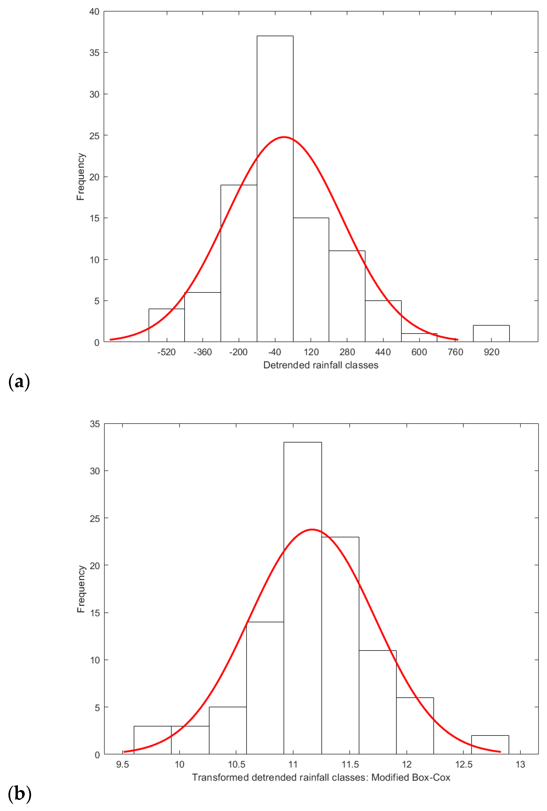
The significant advantage of the Modified Box-Cox method is its application on negative sign data. The detrended data (fluctuations) normality metrics were ${\widehat{k}}_z$ = 5.46 and ${\widehat{s}}_z$ = 0.98, while after the transformation, which calculated λ = 0.12 and α = 23.3, were ${\widehat{k}}_z$ = 4.17 and ${\widehat{s}}_z$ = 0.01. Although the kurtosis coefficient is not very close to the optimum value, it is significantly improved, and the skewness almost fits the optimum value. Figure 3 provides the improvement on the detrended data gaussianity. Moreover, the proposed Modified Box-Cox method provides improved results compared to other transformation functions that treat negative sign data. The complete gaussianity metrics of the original and detrended rainfall data, and of the transformed ones, are presented in Table 2.

The proposed Modified Box-Cox method was also assessed in two more real world cases to demonstrate, in a wider frame, its usefulness. The first accounts for Crete, Greece. The national water monitoring program [28] provides groundwater level information for 311 wells in the area of Crete. Observations include negative sign records (below sea surface) in coastal aquifers. The space-time dataset gaussianity metrics of the original data are: skewness, ${\widehat{s}}_z$ = 2.36 and kurtosis, ${\widehat{k}}_z$ = 9.56, while after transformation with the proposed method are: ${\widehat{s}}_z$ = 0.37 and ${\widehat{k}}_z$ = 3.00, which are very close to the desired gaussian distribution metrics.

A second application refers to petroleum resources evaluation using data of source rocks in the Gulf Coast Basin of Mississippi and Louisiana where 132 samples of Total Organic Carbon wt% were used to test the Modified Box-Cox method efficiency. The data were first detrended using a surface based on their coordinates, therefore, negative sign values were produced. The residuals’ skewness was initially 1.68 and kurtosis 4.86, while after transformation, the metrics were improved to ${\widehat{s}}_z$ = 0.02 and kurtosis, ${\widehat{k}}_z$ = 3.26, very close to the desired gaussian distribution metrics.

In addition, the method was also tested with a random numbers’ generator in MATLAB environment, which is applied very often in simulation tests of field or experimental data for the development of potential realizations, providing also transformation of data very close to the normal distribution. The provided MATLAB code includes also random generator number functions for data reproduction to certify the statement [38]. The available MATLAB function includes a GUI as well, where the initial parameters of minimization function (Equation (7)) can be selected. Furthermore, the Box-Cox setup of the build in MATLAB function is also included for reference application.

Summarizing, real world case studies’ data usually deviate from gaussianity which is very significant in spatial data analysis (variogram calculation) and modeling approaches (uncertainty quantification), and often include negative sign data. Thus, the establishment of a solid function such as the Modified Box-Cox method for reliable gaussian data transformation is important.

4. Conclusions

From a spatial statistics point of view, both Box-Cox and the Modified Method, according to the results, provide transformed data with normality metrics close to the normal distribution values that allows improved dataset properties for spatial interpolation. Therefore, the Modified Box-Cox method consists of an alternative transformation technique that can be applied equally well as the Box-Cox transformation in field measurements and a proposed method for normalization of fluctuations with negative sign. Furthermore, this work showed that the method can be successfully used in different disciplines as well as in synthetic data.

References

- Bostan, P.A.; Heuvelink, G.B.M.; Akyurek, S.Z. Comparison of regression and kriging techniques for mapping the average annual precipitation of Turkey. Int. J. Appl. Earth Obs. Geoinf. 2012, 19, 115–126. [Google Scholar] [CrossRef]
- Theodoridou, P.G.; Varouchakis, E.A.; Karatzas, G.P. Spatial analysis of groundwater levels using Fuzzy Logic and geostatistical tools. J. Hydrol. 2017, 555, 242–252. [Google Scholar] [CrossRef]
- Varouchakis, E.A.; Theodoridou, P.G.; Karatzas, G.P. Spatiotemporal geostatistical modeling of groundwater levels under a Bayesian framework using means of physical background. J. Hydrol. 2019, 575, 487–498. [Google Scholar] [CrossRef]
- Clark, I.; Harper, W.V. Practical Geostatistics 2000; Ecosse North America Llc: Columbus, OH, USA, 2000. [Google Scholar]
- Mcgrath, D.; Zhang, J.E.; Qu, L.T. Temporal and spatial distribution of sediment total organic carbon in an estuary river. J. Environ. Qual. 2004, 35, 93–100. [Google Scholar]
- Gringarten, E.; Deutsch, C.V. Teacher’s aide: Variogram interpretation and modeling. Math. Geol. 2001, 33, 507–534. [Google Scholar] [CrossRef]
- Armstrong, M. Basic Linear Geostatistics; Springer: Berlin, Germany, 1998. [Google Scholar]
- Pardo-Iguzquiza, E.; Dowd, P. Empirical maximum likelihood Kriging: The general case. Math. Geol. 2005, 37, 477–492. [Google Scholar] [CrossRef]
- Goovaerts, P. Geostatistics for Natural Resources Evaluation; Oxford University Press: New York, NY, USA, 1997. [Google Scholar]
- Deutsch, C.V.; Journel, A.G. GSLIB. Geostatistical Software Library and User’s Guide; Oxford University Press: New York, NY, USA, 1992. [Google Scholar]
- Goovaerts, P.; AvRuskin, G.; Meliker, J.; Slotnick, M.; Jacquez, G.; Nriagu, J. Geostatistical modeling of the spatial variability of arsenic in groundwater of southeast Michigan. Water Resour. Res. 2005, 41. [Google Scholar] [CrossRef]
- Asa, E.; Saafi, M.; Membah, J.; Billa, A. Comparison of Linear and Nonlinear Kriging Methods for Characterization and Interpolation of Soil Data. J. Comput. Civ. Eng. 2012, 26, 11–18. [Google Scholar] [CrossRef]
- Varouchakis, E.A.; Hristopulos, D.T.; Karatzas, G.P. Improving kriging of groundwater level data using nonlinear normalizing transformations-a field application. Hydrol. Sci. J. 2012, 57, 1404–1419. [Google Scholar] [CrossRef] [Green Version]
- Wu, X.; Marshall, L.; Sharma, A. The influence of data transformations in simulating Total Suspended Solids using Bayesian inference. Environ. Modell. Softw. 2019, 121, 104493. [Google Scholar] [CrossRef]
- Verdin, A.; Rajagopalan, B.; Kleiber, W.; Funk, C. A Bayesian kriging approach for blending satellite and ground precipitation observations. Water Resour. Res. 2015, 51, 908–921. [Google Scholar] [CrossRef]
- McInerney, D.; Thyer, M.; Kavetski, D.; Bennett, B.; Lerat, J.; Gibbs, M.; Kuczera, G. A simplified approach to produce probabilistic hydrological model predictions. Environ. Modell. Softw. 2018, 109, 306–314. [Google Scholar] [CrossRef]
- Wang, Q.J.; Shrestha, D.L.; Robertson, D.E.; Pokhrel, P. A log-sinh transformation for data normalization and variance stabilization. Water Resour. Res. 2012, 48. [Google Scholar] [CrossRef]
- Varouchakis, E.A.; Hristopulos, D.T.; Karatzas, G.P.; Corzo Perez, G.A.; Diaz, V. Spatiotemporal geostatistical analysis of precipitation combining ground and satellite observations. Hydrol. Res. 2021. [Google Scholar] [CrossRef]
- Wadoux, A.M.J.C.; Brus, D.J.; Rico-Ramirez, M.A.; Heuvelink, G.B.M. Sampling design optimisation for rainfall prediction using a non-stationary geostatistical model. Adv. Water Resour. 2017, 107, 126–138. [Google Scholar] [CrossRef]
- Bárdossy, A.; Pegram, G. Interpolation of precipitation under topographic influence at different time scales. Water Resour. Res. 2013, 49, 4545–4565. [Google Scholar] [CrossRef]
- Markonis, Y.; Batelis, S.C.; Dimakos, Y.; Moschou, E.; Koutsoyiannis, D. Temporal and spatial variability of rainfall over Greece. Theor. Appl. Climatol. 2017, 130, 217–232. [Google Scholar] [CrossRef]
- Iliopoulou, T.; Koutsoyiannis, D.; Montanari, A. Characterizing and Modeling Seasonality in Extreme Rainfall. Water Resour. Res. 2018, 54, 6242–6258. [Google Scholar] [CrossRef]
- Iliopoulou, T.; Koutsoyiannis, D. Projecting the future of rainfall extremes: Better classic than trendy. J. Hydrol. 2020, 588, 125005. [Google Scholar] [CrossRef]
- Malamos, N.; Koutsoyiannis, D. Bilinear surface smoothing for spatial interpolation with optional incorporation of an explanatory variable. Part 2: Application to synthesized and rainfall data. Hydrol. Sci. J. 2016, 61, 527–540. [Google Scholar] [CrossRef]
- Koutsoyiannis, D.; Paschalis, A.; Theodoratos, N. Two-dimensional Hurst–Kolmogorov process and its application to rainfall fields. J. Hydrol. 2011, 398, 91–100. [Google Scholar] [CrossRef]
- Diodato, N. The influence of topographic co-variables on the spatial variability of precipitation over small regions of complex terrain. Int. J. Climatol. 2005, 25, 351–363. [Google Scholar] [CrossRef]
- Ly, S.; Charles, C.; Degré, A. Geostatistical interpolation of daily rainfall at catchment scale: The use of several variogram models in the Ourthe and Ambleve catchments, Belgium. Hydrol. Earth Syst. Sci. 2011, 15, 2259–2274. [Google Scholar] [CrossRef] [Green Version]
- Special Water Secretariat of Greece. National Water Monitoring Network, Groundwater Data, Athens, Greece (In Greek). Available online: http://nmwn.ypeka.gr/?q=groundwater-stations (accessed on 20 October 2020).
- Enomoto, C.; Lohr, C.; Hackley, P.; Valentine, B.; Dulong, F.; Hatcherian, J. Petroleum Geology Data from Mesozoic Rock Samples in the Eastern US Gulf Coast Collected 2011 to 2017. US Geol. Survey Data Release 2018. [Google Scholar] [CrossRef]
- Osborne, J. Improving your data transformations: Applying the Box-Cox transformation. Pract. Assess. Res. Eval. 2010, 15, 12. [Google Scholar]
- Hristopulos, D.T. Random Fields for Spatial Data Modeling; Springer/Nature: Dordrecht, The Netherlands, 2020. [Google Scholar]
- Box, G.E.P.; Cox, D.R. An analysis of transformations. J. R. Stat. Soc. Ser. B 1964, 26, 211–252. [Google Scholar] [CrossRef]
- Sakia, R.M. The Box-Cox transformation technique: A review. JRSSD 1992, 41, 169–178. [Google Scholar] [CrossRef]
- Yeo, I.K.; Johnson, R.A. A new family of power transformations to improve normality or symmetry. Biometrika 2000, 87, 954–959. [Google Scholar] [CrossRef]
- Weisberg, S. Yeo-Johnson power transformations. Dep. Appl. Stat. Univ. Minn. Retrieved June 2001, 1, 2003. [Google Scholar]
- Atkinson, A.B. The box-cox transformation: Review and extensions. Stat. Sci. 2020, 36, 239–255. [Google Scholar]
- Nelder, J.A.; Mead, R. A simplex method for function minimization. Comput. J. 1965, 7, 308–313. [Google Scholar] [CrossRef]
- Varouchakis, E.A. Evarouchakis/Modified-Box-Cox: Modified Box-Cox. Available online: https://zenodo.org/record/4688056#.YIy4jvkzaUk (accessed on 20 October 2020).
Figure 1.
Spatial distribution of the rainfall stations at the island of Crete, Greece.
Figure 2.
Histograms, which fitted the gaussian curve (red), of rainfall data (a) and of transformed values using Box-Cox (b) and Modified Box-Cox (c) methods.
Figure 3.
Histograms, which fitted the gaussian curve (red), of detrended rainfall data (a) and of transformed values (b) using the Modified Box-Cox method.