Efficiency of Intensity Measures Considering Near- and Far-Fault Ground Motion Records

Abstract

This paper focuses on the identification of high-efficiency intensity measures to predict the seismic response of buildings affected by near- and far-fault ground motion records. Near-fault ground motion has received special attention, as it tends to increase the expected damage to civil structures compared to that from ruptures originating further afield. In order to verify this tendency, the nonlinear dynamic response of 3D multi-degree-of-freedom models is estimated by using a subset of records whose distance to the epicenter is lower than 10 km. In addition, to quantify how much the expected demand may increase because of the proximity to the fault, another subset of records, whose distance to the epicenter is in the range between 10 and 30 km, has been analyzed. Then, spectral and energy-based intensity measures as well as those obtained from specific computations of the ground motion record are calculated and correlated to several engineering demand parameters. From these analyses, fragility curves are derived and compared for both subsets of records. It has been observed that the subset of records nearer to the fault tends to produce fragility functions with higher probabilities of exceedance than the ones derived for far-fault records. Results also show that the efficiency of the intensity measures is similar for both subsets of records, but it varies depending on the engineering demand parameter to be predicted.

1. Introduction

Every so often, parts of the Earth are shaken by sudden energy releases, which are associated to the relative movement at the plate boundaries. If the release occurs near human settlements, civil structures can be heavily affected if they are not designed to withstand dynamic horizontal loads. Due to the growth of the world population, in a short time there will hardly be a place where a moderate-to-high earthquake can occur without affecting us. In addition, increasing globalization has produced a redistribution of the risks to society at large. That is, a couple of decades ago, negative consequences of catastrophes barely affected areas other than the stricken one. This is why seismic risk should be a concern of the whole society and not only in the areas with high seismic hazard.

Seismic risk mainly comes from the damage to civil structures. Its extreme consequence for humankind is the collapse of structures, since this leads to the loss of lives, let alone the fact that economical losses can reach the point of affecting the sustainable development of entire countries. Such socio-economical setbacks trigger poverty, inequality, and casualties, amongst many other negative consequences.

According to Coburn and Spence [1], earthquakes up to magnitudes of about 5.5 can occur almost anywhere in the world. These earthquakes can cause damage if they are shallow and trigger significant intensities in areas containing vulnerable structures [2]. However, most of the current seismic hazard maps worldwide have been estimated based on statistical projections, which mostly consider the seismicity recorded just a few decades ago. Hence, several urban environments have been projected without any concern regarding seismic hazard. This has meant that some earthquakes have excessively affected regions rated as relatively low -risk by seismic hazard estimations [3,4].

Trifunac [5] reviewed the history of recording earthquake motions up to the early 1990s. According to this paper, the strong motion instrumentation program in United States started in 1931 (see also [6]). The main purpose was to learn more about the response of structures to seismic actions. An example of the convenience of such data and of the relevance and usefulness of the information they can provide is the paper by Hudson and Housner (1958) [7], who performed a detailed spectrum analysis of the accelerograms corresponding to the 22 March 1957 San Francisco earthquake. In spite of the low Gutenberg–Richter magnitude (5.3), the shaking produced structural damage in the downtown area because of the epicenter proximity. This indicated that the proximity to the rupture plays a paramount role when quantifying seismic risk.

With time, the analysis of ground motions records has also allowed identifying that near-fault events contain severe long duration acceleration pulses, which result in unusually large ground velocity increments [8]. The presence of these pulses can be considered as an important factor in causing damage due to the transmission of a large amount of energy to the structure in a very short time [9]. Thus, the structural response to this type of record has received special attention in recent years; the very large deformation demand on buildings has been of special concern [10,11,12].

This article is focused on two main aspects. The former is to find intensity measures (IMs) exhibiting high efficiency to predict engineering demand parameters (EDPs) when near- and far-fault records are considered. The latter is to quantify the consequences of the increased demand when considering near-fault records in deriving fragility functions. To do so, the probabilistic relationship between seismic hazard in terms of IMs and the structural response in terms of EDPs is studied. This relationship has been an important topic of study in the field of earthquake engineering since several design and assessment methodologies for civil infrastructure are mainly based on the statistical analysis of IM-EDP pairs [13,14,15]. For instance, advanced methodologies to quantify the probability of occurrence of a certain seismic damage state are based on the analysis of these pairs. Therefore, it is a relevant objective to find which IM is best able to predict a specific EDP. Identifying this IM will contribute to reducing uncertainties when quantifying seismic risk of the building stock in human settlements. This reduction is a key aspect to mitigating seismic risk worldwide since stakeholders as well as policy- and decision-makers could prioritize actions to eradicate this risk based on more reliable estimations.

Regarding physical magnitudes to be represented by IMs, displacement, velocity, acceleration, and energy are expected to be highly correlated with the ground motion-induced deformation field of the structure.

Three types of IMs are analyzed herein. The first one is related to the dynamic response of a set of single degree of freedom systems (SDoF) against a certain ground motion record. These IMs are estimated from the spectral response in acceleration, velocity, or displacement.

The second type are IMs obtained from the elastic input energy equivalent velocity spectrum, which is related to the energy input to the structure. This spectrum has recently received research attention since several studies have demonstrated its high effectiveness in the prediction of the seismic structural response [16,17,18,19].

The third type are IMs that can be calculated directly from the ground motion record. To this category belong IMs obtained from computations of the earthquake record such as peak response parameters. The appeal of these IMs is that they do not consider the dynamic properties of the structures like the preceding categories do.

When analyzing the seismic response of civil infrastructure, the most desirable feature for EDPs is that they quantify as best as possible the expected damage. There are many statistical approaches to extract information from IM-EDP pairs on the expected damage to buildings [20,21,22,23,24]. Roughly, the main differences between them lie in the sampling strategy considered to obtain these pairs, the selection procedure of the earthquake records, and the IM and EDP variables selected. The main results of these studies suggest that the most suitable IMs to analyze the probability distribution of an EDP depend on the structural type and the seismogenic environment under consideration.

IMs and EDPs are random variables with a high dispersion. In the case of IMs, this variability is due to the fact that an earthquake generates several types of waves that travel through a very heterogeneous medium at different velocities. The resulting chaotic waves simultaneously influence the position of points located at ground level. It is worth noting that local effects, as well as interaction with civil structures, can also increase the variability observed in IMs.

Regarding EDPs, the randomness may come from the dynamic properties of the structure, which are mainly determined by the type of resistant system against horizontal loads, mechanical properties of the materials, geometric characteristics, acting loads, amongst other aspects [25].

IM-EDP pairs exhibiting high levels of correlation are suitable candidates to analyze the expected damage of buildings subject to ground motions. This is because fragility functions obtained through these highly correlated pairs will exhibit less variability when determining the probability of exceeding a certain damage level assumed as a limit state. IMs can also be used to predict expected values of EDPs [26]. The higher the correlation between an IM and an EDP, the more reliable the estimation of the EDP through an IM. In other words, the most efficient IM to predict an EDP is the one maximizing the correlation between them.

Efficiency of IMs can be measured by considering several sources of uncertainty. For instance, if a specific structure is analyzed, uncertainties related to the mechanical properties of the materials and seismic action are the ones carrying more variability into the response [22,24,27]. For the case of urban environments, information related to the geometrical distribution of buildings belonging to the emplacement are also required [28]. When this geometrical distribution is considered, new properties between variables characterizing hazard and exposure can be analyzed. Within the framework of the KaIROS project (https://cordis.europa.eu/project/id/799553, accessed on 27 May 2021) several numerical tools to deal with such uncertainties have been developed to date. These tools are used herein to analyze the bivariate correlation between a group of IMs and EDPs. To do so, a set of probabilistic numerical 3D models representing the behavior of reinforced concrete (RC) frame buildings is used as a test bed [26].

In order to characterize the seismic action, two subsets of ground motion records are selected. The main difference between them is the distance to the epicenter. These records are scaled with respect to a specific IM so that both subsets have similar intensity values. This can be achieved by defining the same intervals to limit the IM considered. This scaling procedure is intended to produce a building response within and beyond the elastic limit while highlighting the influence of each type of records on the structural performance. Note that for all intervals, the number of records that belong to them is the same.

Once building models and seismic action have both been characterized, several EDPs are obtained through nonlinear dynamic analysis (NLDA). From each subset of ground motion records, a group of IMs are obtained and correlated with the EDPs. Two main aspects will be analyzed: (i) the efficiency of each IM to predict EDPs and (ii) how much the structural response increases in terms of some EDP due to the proximity to the source of the records. The consequences of this increased demand are analyzed through the derivation of fragility functions.

2. Probabilistic Characterization of the Structural Models

In the design of new structures or in the assessment of existing ones, two key issues are the characterization of the seismic hazard and the quantification of the structural response. Both are highly random and should be analyzed from a probabilistic perspective.

Developing proper building models mainly depends on the available information regarding the mechanical and geometrical properties of their structural elements. If buildings of a specific urban environment require analysis, it is also important to know the distribution of as many physical properties as possible (number of structures belonging to each structural type, distribution of the number of stories and spans, acting loads, variability of the mechanical and geometrical properties of the elements, the azimuthal position, amongst many other aspects). In the following, consideration of several of these random variables is explained.

2.1. Epistemic Uncertainties in Structural Input Variables

Several random variables should be considered when the seismic behavior of a group of buildings is modelled. Herein, gravity loads as well as mechanical properties of the materials are considered as random variables. Live loads, LL, permanent loads, DL, the concrete compressive strength, fc, the yield strength of the steel, fy, the elastic modulus of the concrete, Ec, and the elastic modulus of the steel, Es, are considered as random variables. A continuous Gaussian distribution is assumed for them. The coefficient of variations for DL and LL have been set to 0.12 and 0.18, respectively [29]. The coefficient of variation of the concrete compressive strength, fc, may vary from building to building, in the range of 0.07–0.2. The average value of this COV is about 0.15. However, this value depends on the quality control carried out during construction. For instance, a highly controlled concrete tends to exhibit a COV value close to 0.1 [29]. In this study, the COV for the concrete properties has been assumed to be 0.1. Note that the uncertainty level related to the steel is lower than the one considered for the concrete. This is because the quality control of this material is generally superior to that of concrete. Thus, the coefficient of variation of the steel properties has been set to 0.07.

2.2. Geometrical Properties

Vargas-Alzate et al. [26] developed an algorithm that can be used to generate probabilistic MDoF systems representing the behavior of 2D RC frame buildings. This algorithm can be easily adapted to analyze the seismic response of other structural types located in other seismic environments [30]. In this research, this computational tool has been adapted to simulate 3D RC frame buildings having similar characteristics to those projected to meet the requirements of a moderate-to-high seismic area.

The algorithm allows considering several geometrical properties as random variables. Specifically, the number of stories, $N_{st}$, number of spans, $N_{sp}$, story height, $H_{st}$, and span length,$S_l$, can be considered as random variables. For the hypothetical case of study, $N_{st}$ and $N_{sp}$ follow a uniform discrete distribution in the interval (3, 13) and (3, 6), respectively; $H_{st}$ and $S_l$ are distributed uniformly in the interval (2.8, 3.2) m and (4, 6) m, respectively. The aforementioned properties are assumed to be the same for both main directions.

In order to assign the cross-sectional properties of the first story columns of each model, the following equation has been used:

$$W_c or D_c=c_1\ast \ln \left(N_{st}\right)+c_2\ast S_l+c_3{\ast \mathsf{\Phi }}_{1,0}+c_4$$

(1)

where c_i are coefficients that may be adjusted depending on the data distribution of the analyzed area. For this study, $c_1=$ 0.4, $c_2=$ 0.05, $c_3=$ 0.01 and $c_4=$ −0.35. Φ_1,0 is the standard normal distribution. Note that the columns are not necessarily square, that is, one random sample is generated for the width $W_c$ and one for the depth $D_c$ of the columns (Equation (1)). For upper stories, the columns’ size decreases systematically by 5 cm every 3 stories. Values generated according to Equation (1) are rounded to the nearest multiple of 5 cm to be consistent with real dimensions of RC elements.

The width of the beams, $W_b$, depends on the number of stories of the building model and on the span length, and is calculated using the following equation:

$$W_b=b_1\ast N_{st}+b_2\ast S_l+b_3$$

(2)

where b_n are again coefficients that depend on the characteristics of the urban area. For the hypothetical case of study, $b_1=$ 0.01, $b_2=$ 0.02 and $b_3=$ 0.19. Analogously, the depth of the beams, $D_b$, is obtained using the following equation:

$$D_b=g_1\ast N_{st}+g_2\ast S_l+g_3$$

(3)

where $g_1=$ 0.01, $g_2=$ 0.05 and $g_3=$ 0.17. Notice that no random term was considered for the beams.

According to the approach described above, building models have been generated to analyse the relationship between IMs and EDPs from a probabilistic perspective. For the case of near-fault records, 444 building models have been generated while for far-fault records 492. These numbers are in accordance with the availability of records within the analyzed database, as it will be shown below. Figure 1 shows 100 simulated building models according to the description presented above.

As commented above, coefficients considered in equations 1 to 3 as well as the mechanical properties values (

Table 1. Mean, standard deviation and coefficient of variation of the random variables.

Variable	µ (kPa)	σ (kPa)	COV
Dead Loads (DL)	6	0.72	0.12
Live loads (LL)	1	0.18	0.18
Concrete compressive strenght (fc)	2.50 × 104	2.50 × 103	0.10
Yield strength of steel (fy)	4.60 × 105	3.20 × 104	0.07
Elastic modulus of concrete (Ec)	2.30 × 107	2.30 × 106	0.10
Elastic modulus of steel (Es)	2.18 × 108	1.52 × 107	0.07

) have been selected to approximate the expected behavior of RC structures located in earthquake-prone areas. In order to verify this, the fundamental period of the generated models is compared with the approximation given by the European seismic design regulations [31]

$$T_f=0.75H^{0.75}$$

(4)

where $T_f$ represents the fundamental period of the structure and $H$ is the height of the building. Figure 2a shows the comparison between the fundamental period of the generated models for the near-fault case and the expression provided by this regulation. It can be seen that values agree with those expected for the typology analyzed. In order to quantify the dissimilarity between the horizontal stiffness of the 3D models, the following dissimilarity ratio (see Figure 2b) is calculated:

$$R_{Txy}=\frac{T_{x,1}}{T_{y,1}}$$

(5)

3. Seismic Hazard

One of the main sources of uncertainty in estimations of the seismic response of structures is the random variability of the ground motions. There are several methodologies to properly select ground motion records from a database that are consistent with the site-dependent spectral shape [32]. For the purpose of this study, the most important requirement for selecting both subsets of as-recorded accelerograms (near-and far-fault records) is the distance to the epicenter. These records have been selected from the Engineering Strong Motion Database compiled by the ‘Instituto Nazionale di Geofisica e Vulcanologia’, INGV [33]. The first subset is composed by 444 records whose distance to the epicenter is lower than 10 km, while the second subset contains 492 records whose distance to the epicenter is within the interval 10–30 km.

To scale the selected records, the objective is that the structural models reach different performance levels. It is also a requirement that each subset be scaled to have IM values similar to each other. However, the availability of strong ground motion records covering high-intensity intervals at specific periods is a common restriction found in current databases. This lack of strong ground motion records can trigger excessive scaling to fit within high-intensity intervals. It is worth mentioning that, for the purpose of this study, it should be avoided to scale the same record to different intensity levels since this introduce false correlation between IMs and EDPs. In order to face these issues, the following procedure has been used for selecting and scaling (where necessary) each subset of records:

• Classify the ground motion records according to the distance to the epicenter.
• Identify the IM for selecting ground motion records.
• Define the IM intervals.
• Calculate the selected IM for the entire set of records that belong to the database.
• Sort the ground motion records in descending order as a function of the IM value calculated in step 4.
• The ground motion record with the highest IM is scaled so that its new IM value belongs to the highest interval. If the IM naturally fulfils the interval condition, no scale factor is considered. This step is repeated with the subsequent IMs, according to the sorted list, until the desirable number of records belonging to the highest interval is obtained.
• Step 6 is repeated for all intervals. The scale factor in step 6 is calculated having in mind that the IM values are uniformly distributed within each interval.

It is important to select an IM (Step 2) highly correlated with the structural response. That is, an IM (or an arrangement of them) capable of predicting specific EDPs. Hence, it is more adequate to look into IMs calculated from the spectral response of single-degree-of-freedom systems, SDoF, as they have proven to be highly correlated with the structural response in terms of EDPs [34]. In this respect, several researchers have proven that it is more efficient to use IMs based on average spectral values around the fundamental period of the structure than using the spectral value associated to it [35,36,37,38,39]. However, because of the probabilistic approach of this study, there is not a single structural model, but a group of them which, in addition, have highly variable fundamental periods (see Figure 2a). Therefore, the period range for averaging spectral ordinates is established from the dynamic properties of the entire population of buildings [26]. In this way, earthquake records within each preselected subset are scaled so that their mean spectral accelerations, in the interval (0.2–1.6) s, meet the scaling criteria presented above. The intensity levels defining the upper and lower limits of each band range from 0.035 to 0.7 g at intervals of 0.035 g. Figure 3a shows the geometric mean spectra of the horizontal components of 444 scaled near-fault records while Figure 3b shows the same spectra for the 492 scaled far-fault records.

Figure 3c shows a comparison between the mean value of each subset. It can be seen that, for periods lower than approximately 0.45 s, the mean spectrum of the near-fault records is higher than the mean one for far-fault records and that the opposite happens for periods higher than 0.45 s (see Figure 3d).

4. Intensity Measures

IMs can be obtained ranging from the subjective opinion of people who felt the acceleration produced by the ground motion to those calculated from signals recorded by sophisticated devices measuring acceleration amplitudes which humans are not able to detect. Prior to the development of seismological networks worldwide, there was scarce information on the characteristics of ground motion produced by earthquakes. Nowadays, these complex and interactive networks have provided humankind with valuable datasets, allowing to enhance the interpretation of the effect of seismic waves in urban environments. These networks are continuously recording three orthogonal acceleration components at the ground level in several places across the planet. Such records implicitly contain information about the interaction of physical processes of highly random variability. Basic mathematical background along with proper numerical tools allow extracting from these records variables representing the seismicity of an area. In the context of earthquake engineering, such variables are known as instrumental IMs. Ideally, an IM should contain enough information about the earthquake, so according to it, the structural response can be predicted with confidence [40]. Notice that an IM can depend either on the earthquake properties, or on both the earthquake and structural features [38].

From the statistical point of view, one of the most desirable features that an IM should exhibit is efficiency [41,42,43]. An IM is considered efficient if it reduces the dispersion in the estimated parameter representing the structural response. An IM exhibiting efficiency could potentially reduce the number of structural calculations in estimations of seismic risk at the urban level.

4.1. Spectral-Based Intensity Measures

The dynamic response of structures subject to earthquakes has been correlated to the peak response of an equivalent SDoF system. The study of this simplified model gives rise not only to the response spectra but also to spectral IMs. It has been recognized that efficient IMs would be defined by response spectral ordinates [26]. This is why response spectral ordinates are extensively used to quantify the seismic hazard at a site. Such ordinates are obtained from the dynamic equilibrium equation for SDoF systems:

$$m{\ddot{u}}_n\left(t\right)+c{\dot{u}}_n\left(t\right)+k{u}_n\left(t\right)=-m{\ddot{u}}_{g,n}\left(t\right)$$

(6)

where ${\ddot{u}}_n\left(t\right)$, ${\dot{u}}_n\left(t\right)$, and $u_n\left(t\right)$ are the spectral acceleration, velocity and displacement time history responses of the SDoF in the n direction, respectively; ${\ddot{u}}_{g,n}\left(t\right)$ is the acceleration ground motion; m, c, and k represent the mass, damping, and stiffness of the system, respectively. IMs from 1 to 6 described in

Table 2. Intensity measures description.

Intensity Measure	Id	Formula 1D 1	Formula 2D 2
Spectral acceleration at $T_{n,j}$	1	$S{a}_n\left(T_{n,j}\right)=\max \left(\left|{\ddot{u}}_{g,n}\left(t\right)+{\ddot{u}}_n\left(T_{n,j}\right)\right|\right)$	$Sa=\sqrt{S{a}_x\left(T_{x,j}\right)\ast S{a}_y\left(T_{y,j}\right)}$
Spectral velocity at $T_{n,j}$	2	$S{v}_n\left(T_{n,j}\right)=\max \left(\left|{\dot{u}}_n\left(T_{n,j}\right)\right|\right)$	$Sv=\sqrt{S{v}_x\left(T_{x,j}\right)\ast S{v}_y\left(T_{y,j}\right)}$
Spectral displacement at $T_{n,j}$	3	$S{d}_n\left(T_{n,j}\right)=\max \left(\left|u_n\left(T_{n,j}\right)\right|\right)$	$Sd=\sqrt{S{d}_x\left(T_{x,j}\right)\ast S{d}_y\left(T_{y,j}\right)}$
Average spectral acceleration 3,4	4	$AvS{a}_n=\frac{{{\displaystyle \sum }}_{i=1}^{n_T}S{a}_n\left(T_i\right)}{n_T}$	$AvSa=\sqrt{AvS{a}_x\ast AvS{a}_y}$
Average spectral velocity	5	$AvS{v}_n=\frac{{{\displaystyle \sum }}_{i=1}^{n_T}S{v}_n\left(T_i\right)}{n_T}$	$AvSv=\sqrt{AvS{v}_x\ast AvS{v}_y}$
Average spectral displacement	6	$AvS{d}_n=\frac{{{\displaystyle \sum }}_{i=1}^{n_T}S{d}_n\left(T_i\right)}{n_T}$	$AvSd=\sqrt{AvS{d}_x\ast AvS{d}_y}$
Equivalent velocity at $T_{n,j}$	7	$V{E}_n\left(T_{n,j}\right)=\sqrt{2E_{I,n}\left(T_{n,j}\right)}$	$VE=\sqrt{V{E}_x\left(T_{x,j}\right)\ast V{E}_y\left(T_{y,j}\right)}$
Average equivalent velocity	8	$AvV{E}_n=\frac{{{\displaystyle \sum }}_{i=1}^{n_T}VE\left(T_i\right)}{n_T}$	$AvVE=\sqrt{AvV{E}_x\ast AvV{E}_y}$
Peak ground acceleration	9	$PG{A}_n=\max \left(\left|{\ddot{u}}_{g,n}\left(t\right)\right|\right)$	$PGA=\sqrt{PG{A}_x\ast PG{A}_y}$
Peak ground velocity	10	$PG{V}_n=\max \left(\left|{\dot{u}}_{g,n}\left(t\right)\right|\right)$	$PGV=\sqrt{PG{V}_x\ast PG{V}_y}$
Peak ground displacement	11	$PG{D}_n=\max \left(\left|u_{g,n}\left(t\right)\right|\right)$	$PGD=\sqrt{PG{D}_x\ast PG{D}_y}$
Specific Energy Density [46,47]	12	${SED}_n={{\displaystyle \int }}_{t_i}^{t_f}{\dot{u}}_{g,n}{\left(t\right)}^2 dt$	$SED=SE{D}_x+SE{D}_y$
Arias intensity [48]	13	$I_A{}_n=\frac{\pi }{2 g}{{\displaystyle \int }}_{t_i}^{t_f}{\ddot{u}}_{g,n}{\left(t\right)}^2 dt$	$I_A=I_A{}_x+I_A{}_y$
Characteristic intensity [49]	14	$I_c{}_n=ac{c}_{RMS}{{}_n}^{1.5} \sqrt{{\Delta }_n}$	$I_C=I_C{}_x+I_C{}_y$
Root mean of the velocity 5	15	$ve{l}_{RMS}{}_n=\sqrt{\frac{1}{{\Delta }_n}{{\displaystyle \int }}_{t_{5\%}}^{t_{95\%}}{\dot{u}}_{g,n}{\left(t\right)}^2 dt}$	$ve{l}_{RMS}=ve{l}_{RMS}{}_x+ve{l}_{RMS}{}_y$
Root mean of the acceleration [50]	16	$ac{c}_{RMS}{}_n=\sqrt{\frac{1}{{\Delta }_n}{{\displaystyle \int }}_{t_{5\%}}^{t_{95\%}}{\ddot{u}}_{g,n}{\left(t\right)}^2 dt}$	$ac{c}_{RMS}=ac{c}_{RMS}{}_x+ac{c}_{RMS}{}_y$
Cumulative Absolute Velocity [51]	17	$CA{V}_n={{\displaystyle \int }}_{t_i}^{t_f}\left|{\ddot{u}}_{g,n}\left(t\right)\right| dt$	$CAV=CA{V}_x+CA{V}_y$
Fajfar intensity [52]	18	$I_F{}_n=PG{V}_n{\Delta }_n{}^{\beta }$	$I_F=\sqrt{I_F{}_x\ast I_F{}_y}$

¹ 1D stands for 1 horizontal dimension. ² 2D stands for 2 horizontal dimensions. ³ $T_i$ represents a vector of periods around the fundamental period of the structure. ⁴ $n_T$ is the length of $T_i$. ⁵ ${\Delta }_n$ is the significant duration of the record in the n direction.

belong to this category.

4.2. Energy-Based Intensity Measures

For both design and assessing the performance of civil structures, the peak response of physical magnitudes like displacement, velocity or acceleration has been widely used. However, several researchers have found that the expected damage of structures can be strongly tied to the amount of energy introduced to the system [16,17,18,19]. In this respect, the equivalent velocity spectrum represents the amount of energy introduced to a set of SDoF systems. This energy can be calculated by rewriting equation 6 in terms of energy. That is, each term of this equation is multiplied by the differential increment of displacement $({\dot{u}}_{n}dt$) and then integrating in the time interval (0, t), as follows [44,45]:

$$m{{\displaystyle \int }}_0^t{\ddot{u}}_n{\dot{u}}_{n}dt+c{{\displaystyle \int }}_0^t{\dot{u}}_n^{2}dt+k{{\displaystyle \int }}_0^t{u}_n{\dot{u}}_{n}dt=-m{{\displaystyle \int }}_0^t{\ddot{u}}_{g,n}{\dot{u}}_{n}dt$$

(7)

where $E_{k,n}=m{{\displaystyle \int }}_0^t{\ddot{u}}_n{\dot{u}}_{n}dt$ is the kinetic energy; $E_{\xi ,n}=c{{\displaystyle \int }}_0^t{\dot{u}}_n^{2}dt$ is the energy dissipated by the inherent damping; $E_{a,n}=k{{\displaystyle \int }}_0^t{u}_n{\dot{u}}_{n}dt$ is the energy absorbed by the system; and $E_{I,n}=-m{{\displaystyle \int }}_0^t{\ddot{u}}_{g,n}{\dot{u}}_{n}dt$ is the energy introduced into the system by the ground motion. The latter term is commonly expressed in terms of equivalent velocity, $VE$, and is normalized with respect to the mass of the structure:

$$V{E}_n=\sqrt{2E_{I,n}\left(T_{n,j}\right)}$$

(8)

Calculating $V{E}_n$ for several elastic oscillators will produce the equivalent velocity spectrum. IMs 7 and 8 described in Table 2 are obtained from the energy introduced into the system.

4.3. IMs Based on Direct Computations of the Ground Motion Record

IMs presented above use the spectral response of SDoF systems. However, several IMs are obtained from direct computations of the ground motion record. The appeal of this type is that they do not depend on the dynamic properties of the structures. In this way, a generic fragility function could be developed to estimate the seismic performance of buildings with very different structural properties. However, such independency causes a decrease of the efficiency for predicting EDPs, as shown later on. IMs from 9 to 18 described in Table 2 belong to this category. Note that these IMs are generally computed as the sum of the IM values calculated for each component of the record.

5. Engineering Demand Parameters

Engineering demand parameters are used to design or assess the expected behavior of buildings. The most desirable feature for EDPs is that they quantify as best as possible the performance level of structures subject to ground motions. One of the most used EDP for estimating this level is the maximum inter-storey drift ratio, MIDR [53]. Many other variables like the maximum displacement of the roof, maximum global drift ratio or the base shear coefficient can be considered as EDP. Herein, EDPs have been calculated as the combined response in the main direction of the structure. In the following section, several EDPs are briefly described.

5.1. Maximum Displacement at the Roof ($\delta r$)

The maximum displacement at the roof, $\delta r$, is an EDP highly used in the capacity spectrum method [54]. In the case of NLDA, this EDP can be estimated as follows:

$$\delta r=\max \left(\sqrt{\delta r_x^2\left(t\right)+\delta r_y^2\left(t\right)}\right)$$

(9)

where $\delta r_x\left(t\right)$ and $\delta r_y\left(t\right)$ are the displacement at the roof level in each principal direction.

5.2. Maximum Global Drift Ratio (MGDR)

Maximum Global Drift Ratio is mostly used as a representative quantity for determining the general performance of structures when subjected to earthquakes [55]. This EDP can be obtained by dividing $\delta r$ between the height of the building:

$$\mathrm{MGDR}=\frac{\delta r}{H}$$

(10)

5.3. Maximum Inter-Storey Drift Ratio (MIDR)

As said in the preceding, the MIDR is probably the most used EDP when analyzing buildings subject to horizontal ground motions. This EDP is highly used in both designing or assessing the vulnerability of buildings. For storey i, the evolution of the inter-storey drift is given by:

$$ID{R}_{i,n}\left(t\right)=\frac{{\delta }_{i,n}\left(t\right)-{\delta }_{i-1,n}\left(t\right)}{h_i}$$

(11)

where ${\delta }_{i,n}\left(t\right)$ is the displacement at the floor i of the structure; $h_i$ represents the height of the storey i. The maximum inter-storey drift ratio at the storey i, $MID{R}_i$, can be calculated as follows:

$$MID{R}_i=\max \left(\sqrt{ID{R}_{i,x}^2\left(t\right)+ID{R}_{i,y}^2\left(t\right)}\right)$$

(12)

In order to estimate the damage level of the most affected storey, the maximum inter-storey drift ratio observed in the building, MIDR, is given by:

$$MIDR=\max \left[MID{R}_1,MID{R}_2\dots MID{R}_{N_{st}}\right]$$

(13)

5.4. Base Shear Coefficcient ($CS)$

In order to quantify the amount of force acting on the columns located at the ground level of the structure, the base shear coefficient (see Equation (14)) is calculated as the ratio between the combination of the maximum base shear in each direction and the total weight of the building, W. This coefficient is of paramount importance when designing civil structures to withstand seismic-induced effects.

$$CS=\frac{\max \left(\sqrt{V_x^2\left(t\right)+V_y^2\left(t\right)}\right)}{W}$$

(14)

where $V_x\left(t\right)$ and $V_y\left(t\right)$ are the base shear in each principal direction.

6. Statistical Analysis of IM-EDP Pairs

Mostly, seismic risk comes from the damage occurred to civil structures after an earthquake. This damage appears when the elastic response of the structural and non-structural elements is exceeded. There are many numerical methods to estimate this nonlinear dynamic response. They range from adapted linear-static-based-methods to more advanced ones, considering the nonlinear static (pushover-based methods) or dynamic response of a structure (NLDA). This latter is the most reliable numerical tool to simulate the nonlinear dynamic response of buildings.

Two sets of NLDAs are performed in this research. The first one considers as seismic hazard the selected near-fault records whilst the latter the far-fault ones. The Ruaumoko software has been used to perform the structural analyses [56]. From these calculations, the IMs and EDPs presented in Section 4 and Section 5, respectively, are obtained. The correlation coefficient, $R^2$, of the resulting cloud of IM-EDP points is estimated so that the most efficient IM can be identified.

6.1. Analysis of IMs Efficiency

In this study, IM-EDP relationships are characterized by performing a nonlinear regression analysis in the log-log space. As with linear least squares, nonlinear regression is based on determining the values of the parameters that minimize the sum of the squares of the residuals. In this sense, the following general linear least-square model allows several types of regression:

$$y={\displaystyle \sum }_{i=1}^{m+1}{\alpha }_{i-1}{z}_{i-1}+\epsilon$$

(15)

where ${\alpha }_0$, ${\alpha }_1$, …${\alpha }_m$ are the coefficients providing the best fit between model and data; $z_0$, $z_1$, …$z_m$ are m+1 basis functions; $\epsilon$ represents the residuals. It can easily be seen how polynomial regression falls within this model. That is, $z_0=1$, $z_1=x$, …$z_m=x^m$. Substituting in equation 15 $y=\ln EDP$ and $z_{i-1}={\left(\ln IM\right)}^{i-1}$, the linear least-square model using polynomial functions can be used to extract statistical information from IM-EDP pairs according to the following expression:

$$\ln EDP={\displaystyle \sum }_{i=1}^{m+1}{\alpha }_{i-1}{\left(\ln IM\right)}^{i-1}+\epsilon$$

(16)

For m = 2, this equation adopts the following quadratic form:

$$\ln EDP={\alpha }_0+{\alpha }_1\ln IM+{\alpha }_2{(\ln IM)}^2+\epsilon$$

(17)

where ${\alpha }_0$, ${\alpha }_1,$ and ${\alpha }_2$ are scalars maximizing $R^2$ for IM-EDP pairs. Further information regarding the development and implementation of this type of polynomial models in the log-log space can be found in [57]. For a perfect fit, $R^2$ = 1, signifying that the quadratic function explains 100% of the variability of the data.

$R^2$ is used herein to provide an estimation of the variability when analyzing IM-EDP pairs. That is, the higher $R^2$, the lower the variability when predicting some EDP given an IM. Consequently, the IM providing the highest $R^2$ will be the most efficient one. Note that the quadratic arrangement described above allows to fit linear functions if that is what the data suggests. For these cases, ${\alpha }_2$ tends to zero.

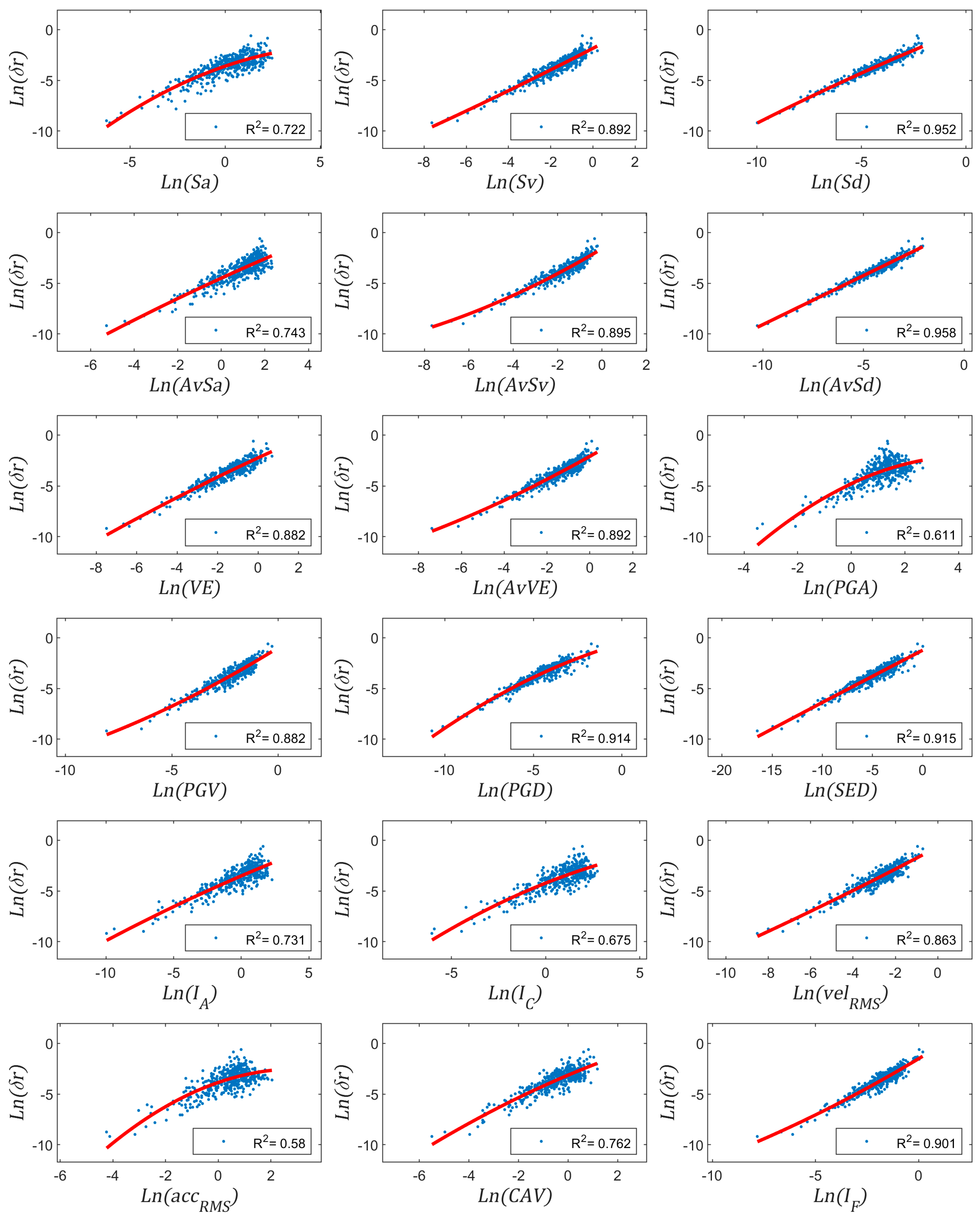
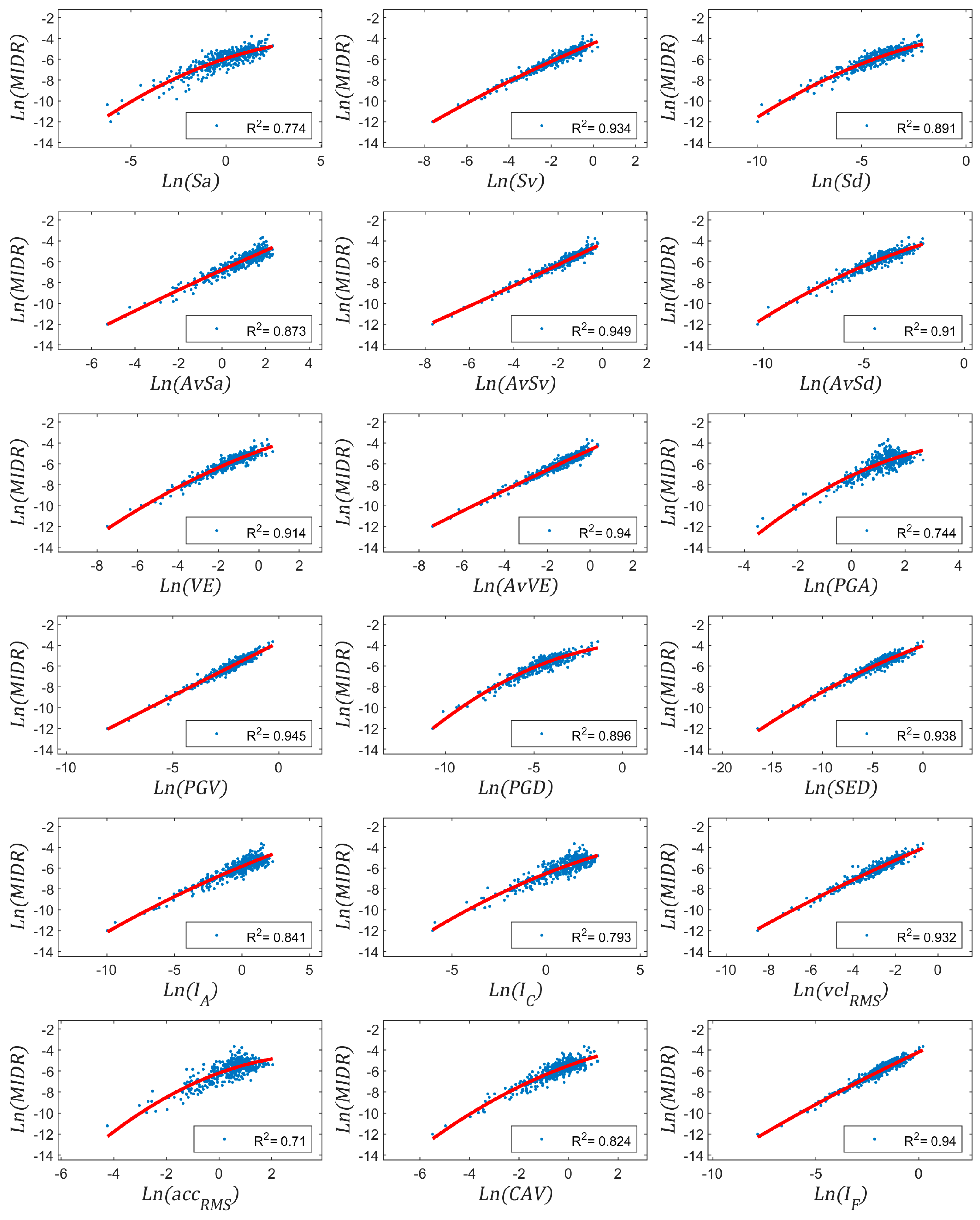
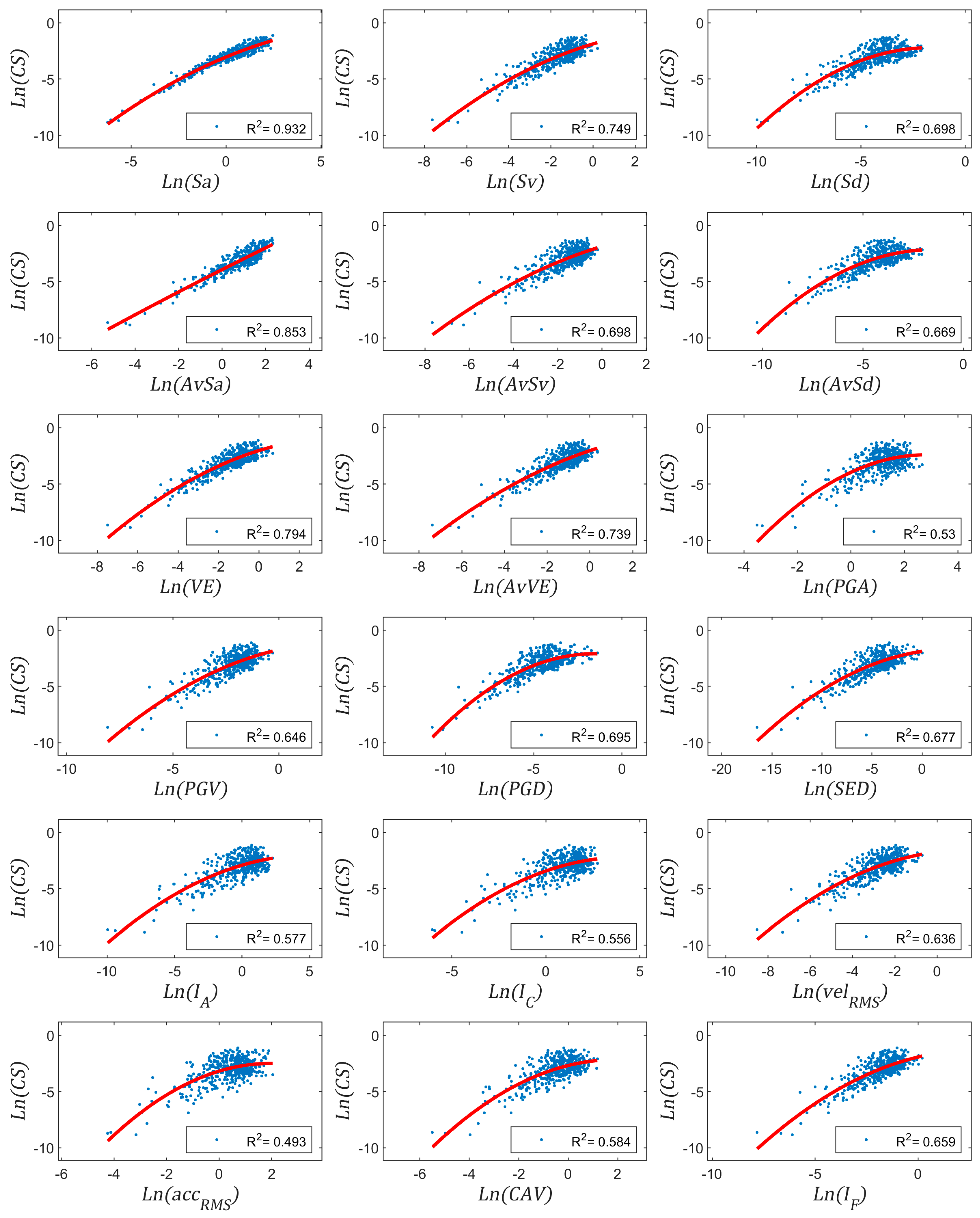
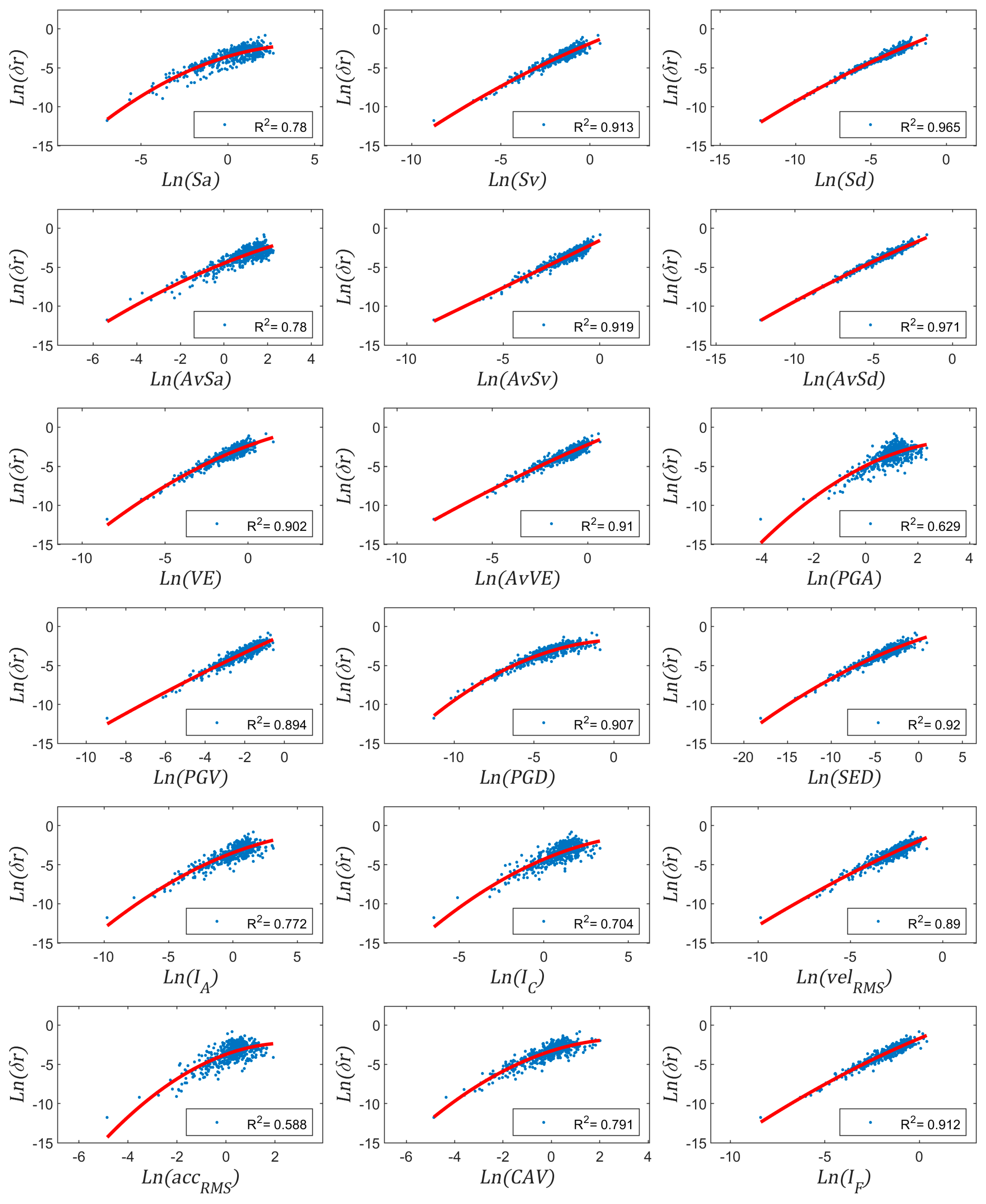
In the following, variables described in Section 4 and Section 5 are used as IMs and EDPs, respectively. Note that most of the simulations performed in this study fell within the nonlinear range. This is not a coincidence but a consequence of the scaling values of the ground motion records. Figure 4, Figure 5, Figure 6 and Figure 7 show the relationships in the log-log space between EDPs and IMs considering near-fault records. Figure 8, Figure 9, Figure 10 and Figure 11 show analogous data for far-fault records.

6.2. Near-Fault Ground Motion Records

Figure 4 shows that AvSd exhibits the highest ability to predict δr for near-fault ground motion records. It is worth noting that the relationship between both variables in the log-log space seems linear. In general, IMs based on displacement are the ones most correlated to δr. Regarding the group of IMs independent of structural properties, SED is the one with the highest efficiency to predict δr.

VE is the IM that minimizes the dispersion when predicting MGDR (see Figure 5). It is worth mentioning the high efficiency exhibited by the classic Sa, which is even higher than that of AvSa. The latter has been shown to have superior ability to predict MIDR, at least in terms of acceleration-based IMs. Regarding IMs independent of structural properties, PGD is the one with the highest efficiency.

Figure 6 allows to identify that AvSv is the IM exhibiting the highest efficiency for predicting MIDR. In general, it can be seen that velocity-based IMs are the ones most correlated with MIDR. This also occurs when analyzing IMs independent of the structural properties, e.g., PGV, SED, and $ve{l}_{RMS}$. Note that the arrangement originally proposed by Fajfar et al. [50] (i.e., β = 0.25) tends to show less correlation when compared with the PGV, at least when MIDR plays the role of EDP. It has been found that using β = 0.07 provides a better correlation value for this IM ($R^2$ = 0.949).

For the case of CS, Figure 7 shows that the IM most correlated is Sa. Note that the correlation index obtained when relating this IM with CS is significantly higher than the rest of IMs.

6.3. Far-Fault Ground Motion Records

Figure 8 shows that AvSd is again the IM with the highest ability to predict δr. It is also observed that the relationship between both variables in the log-log space seems linear. IMs based on displacement are the ones that exhibit the highest efficiency with respect to δr. From the group of IMs independent of structural properties, SED is again the IM minimizing the dispersion when predicting δr. For the case of MGDR, Sa is the IM that exhibits the highest efficiency (see Figure 9). Regarding IMs independent of structural properties, SED is the one most correlated to MGDR. AvSv is again the IM exhibiting the highest efficiency for predicting MIDR (see Figure 10). In general, it can be seen again that velocity-based IMs are the ones most correlated with MIDR. This also occurs when analyzing IMs independent of the structural properties, e.g., PGV, SED and $ve{l}_{RMS}$. When MIDR plays the role of EDP, the arrangement originally proposed by Fajfar et al. [50] (i.e., β = 0.25) tends to show less correlation when compared with the PGV. It has been found that using β = 0.07 provides a better correlation value for this IM ($R^2$ = 0.949). For the case of CS, Figure 11 shows that the IM most correlated is Sa. Note again that the correlation index obtained when using this IM is significantly higher than the rest of IMs.

6.4. Spearman Coefficcient

It can be argued that $R^2$ is not adequate to explain the causality between IMs and EDPs. This is because the lack of linearity (exhibited between some sets of IM-EDP pairs), normality and homoscedasticity of these variables. Regarding linearity, the quadratic model used to perform the regression analysis overcomes this issue. Regarding normality and homoscedasticity, it has been observed that both types of variables, i.e., IMs and EDPs, tend to be lognormal in the log-log space. This calls into question the use of $R^2$. Therefore, it has been analyzed the Spearman coefficient, ρ, which is an alternative index less sensitive to the lack of such properties. It has been observed that the correlation values are similar between this coefficient and the one emerging from the quadratic regression model. What is most important is that both approaches identify the same IM as the one maximizing the correlation with the specific EDP, as shown in Figure 12 (see blue circles).

In general, slightly higher $R^2$ values are observed for far-fault records. This could be because near-fault records introduce larger demands to the analyzed structures. That is, the higher the nonlinearity the higher the dispersion of the data. In order to analyze the implications of this increased demand, fragility functions may provide valuable information. These curves allow estimating the conditional probability of exceeding a certain damage threshold given an IM value. Note that since both subsets of records were scaled to meet similar IMs, fragility functions that provide the highest probability of exceedance are those that come from the highest demands. In the following section, fragility functions derived from near- and far-fault records are compared.

6.5. Fragility Functions

From the IM-EDP relationships shown in Figure 4, Figure 5, Figure 6, Figure 7, Figure 8, Figure 9, Figure 10 and Figure 11, one can derive fragility functions according to the so-called ‘cloud analysis’ approach [19]. This methodology requires to calculate the best fit curve between a set of IMs and EDPs realizations in the log-log space. The resultant curve is used to calculate the mean of a normal distribution which depends on the IM value. The variability of this distribution is estimated as the standard deviation of the IM-EDP residuals with respect to the fitted curve. Hence, when varying the IM value, the probability of exceeding a specific damage threshold can be estimated. It is worth recalling that these thresholds are particular realizations of the EDP under consideration, EDP_C.

According to the above, the variability of the fragility functions is directly related to the dispersion of the IM-EDP points. The higher this dispersion, the more uncertainty there is when defining whether the structure presents one specific damage state or another. That is why it is important to identify efficient IMs.

In the present study, fragility functions are derived with respect to a regression analysis which allows to consider the non-linear relationship between random variables. This approach renders the estimation of the probability of exceedance more reliable. However, it should be borne in mind that, in low correlation cases, it is not recommended to derive fragility functions using the quadratic approximation since the fitted curve tends to be highly non-linear, thus compromising the quality of the corresponding function.

As discussed above, fragility curves can be used to analyze the consequences of a subset of records that place higher demands on similar structures than another. In other words, the first subset contains more damaging ground motion records than the second one.

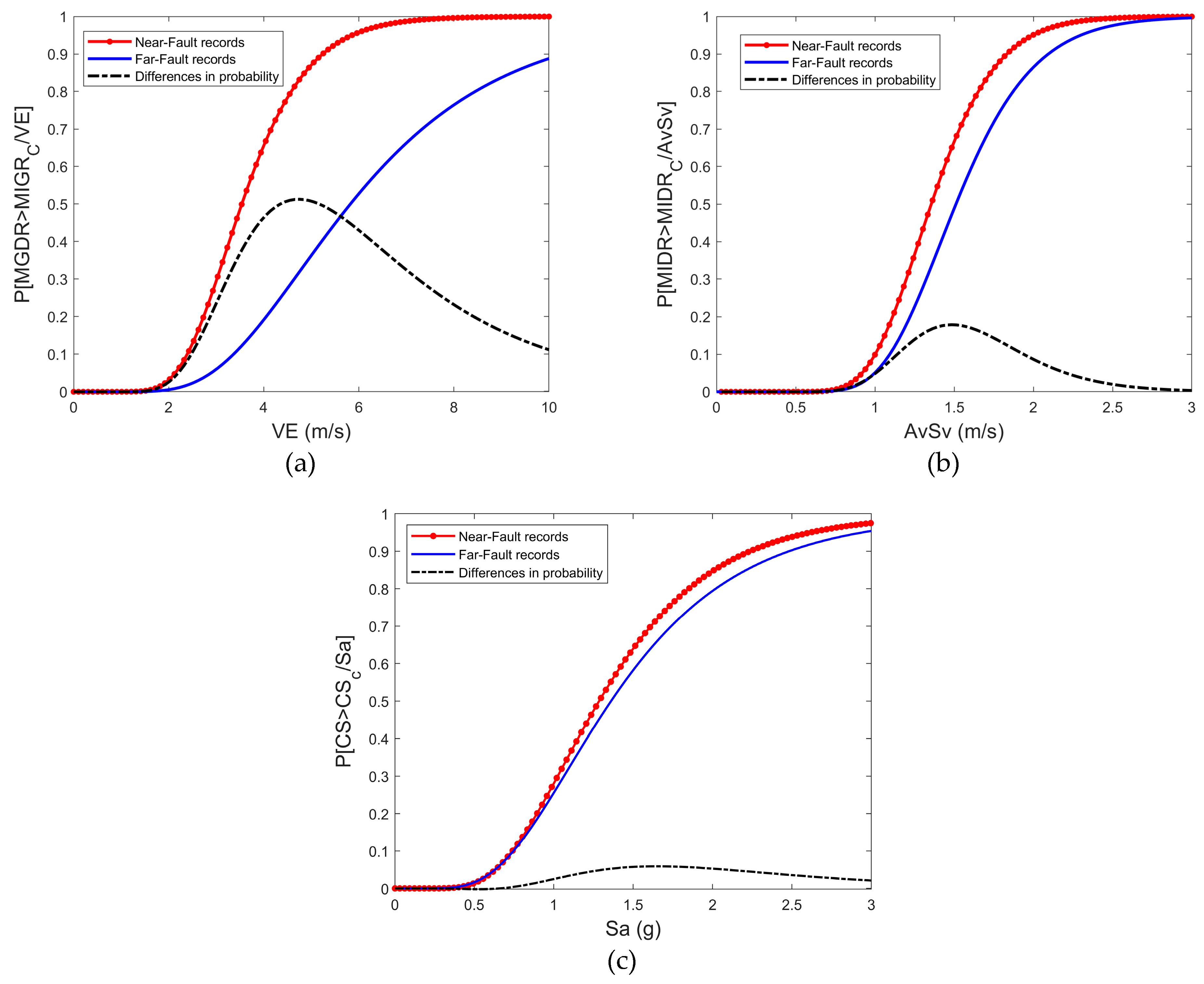
Considering the cloud analysis approach described above, fragility functions for MGDR, MIDR and CS considering near- and far-fault records are derived (see Figure 13). Fragility functions for $\delta r$ have not been calculated due to the high dependency of this EDP on the building’s height.

The IM considered to derive each curve is the one exhibiting the highest correlation with the EDP. In this way, VE, AvSv and Sa have been used to calculate fragility functions for MGDR, MIDR and CS, respectively.

Table 3. Correlation index values. ${\overline{R}}_{NF}^2$ and ${\overline{R}}_{FF}^2$ are the average of the correlation index $R^2$ among all the EDPs analyzed for near-fault and far-fault records, respectively; the highest correlation values are highlighted in red.

	Near-Fault Records				Far-Fault Records				Average Values
	${\mathit{R}}^{\mathbf{2}}\mathbf{\left(}\mathit{\delta }\mathit{r}\mathbf{\right)}$	${\mathit{R}}^{\mathbf{2}}\mathbf{\left(}\mathit{M}\mathit{G}\mathit{D}\mathit{R}\mathbf{\right)}$	${\mathit{R}}^{\mathbf{2}}\mathbf{\left(}\mathit{M}\mathit{I}\mathit{D}\mathit{R}\mathbf{\right)}$	${\mathit{R}}^{\mathbf{2}}\mathbf{\left(}\mathit{C}\mathit{S}\mathbf{\right)}$	${\mathit{R}}^{\mathbf{2}}\mathbf{\left(}\mathit{\delta }\mathit{r}\mathbf{\right)}$	${\mathit{R}}^{\mathbf{2}}\mathbf{\left(}\mathit{M}\mathit{G}\mathit{D}\mathit{R}\mathbf{\right)}$	${\mathit{R}}^{\mathbf{2}}\mathbf{\left(}\mathit{M}\mathit{I}\mathit{D}\mathit{R}\mathbf{\right)}$	${\mathit{R}}^{\mathbf{2}}\mathbf{\left(}\mathit{C}\mathit{S}\mathbf{\right)}$	${\overline{\mathit{R}}}_{\mathit{N}\mathit{F}}^{\mathbf{2}}$	${\overline{\mathit{R}}}_{\mathit{F}\mathit{F}}^{\mathbf{2}}$	$\frac{{\overline{\mathit{R}}}_{\mathit{N}\mathit{F}}^{\mathbf{2}}\mathbf{+}{\overline{\mathit{R}}}_{\mathit{F}\mathit{F}}^{\mathbf{2}}}{\mathbf{2}}$
$Sa$	0.722	0.927	0.774	0.932	0.780	0.947	0.809	0.930	0.839	0.866	0.853
$Sv$	0.892	0.915	0.934	0.749	0.913	0.916	0.936	0.744	0.873	0.877	0.875
$Sd$	0.952	0.894	0.891	0.698	0.965	0.888	0.896	0.687	0.859	0.859	0.859
$AvSa$	0.743	0.889	0.873	0.853	0.780	0.911	0.883	0.862	0.840	0.859	0.849
$AvSv$	0.895	0.880	0.949	0.698	0.919	0.899	0.955	0.707	0.856	0.870	0.863
$AvSd$	0.958	0.881	0.910	0.669	0.971	0.883	0.912	0.668	0.854	0.859	0.856
$VE$	0.882	0.937	0.914	0.794	0.902	0.935	0.915	0.790	0.882	0.886	0.884
$AvVE$	0.892	0.906	0.940	0.739	0.910	0.919	0.938	0.751	0.869	0.879	0.874
$PGA$	0.611	0.586	0.744	0.530	0.629	0.582	0.720	0.487	0.618	0.604	0.611
$PGV$	0.882	0.842	0.945	0.646	0.895	0.856	0.942	0.653	0.829	0.836	0.832
$PGD$	0.915	0.885	0.896	0.695	0.908	0.861	0.872	0.686	0.848	0.832	0.840
$SED$	0.915	0.879	0.938	0.677	0.920	0.882	0.924	0.692	0.852	0.855	0.854
$I_A$	0.731	0.693	0.841	0.577	0.772	0.724	0.831	0.589	0.710	0.729	0.720
$I_C$	0.675	0.642	0.793	0.556	0.704	0.650	0.771	0.535	0.666	0.665	0.666
$ve{l}_{RMS}$	0.863	0.827	0.932	0.636	0.890	0.861	0.940	0.668	0.814	0.840	0.827
$ac{c}_{RMS}$	0.580	0.551	0.710	0.493	0.588	0.541	0.681	0.459	0.583	0.567	0.575
$CAV$	0.762	0.716	0.824	0.585	0.791	0.742	0.807	0.608	0.722	0.737	0.729
$I_F$	0.901	0.860	0.940	0.659	0.912	0.869	0.935	0.666	0.840	0.846	0.843

presents the correlation index values between all the IMs and EDPs, for near- and far-fault records. Average values are also presented (${\overline{R}}_{NF}^2$ and ${\overline{R}}_{FF}^2)$.

In Figure 13, it can be seen that, for all the fragility curves, near-fault records tend to induce larger demands on the analyzed buildings than the far-fault ones. This effect is more conspicuous when analyzing MGDR, reaching differences in probabilities in the order of 0.5. For MIDR, these differences may reach values in the order of 0.18. For CS, the observed differences are significantly lower (0.06). The damage thresholds were established at MIGR_C = 0.02, MIDR_C = 0.02, and CS_C = 0.3.

7. Concluding Remarks

It has been observed that a single IM is not able to predict, with the highest efficiency, all the EDPs considered in this research. This means that depending on the EDP to be studied, it is more convenient to use one IM or another. However, a general efficiency can be estimated by averaging all the $R^2$ associated to each IM-EDP set of points. This average coefficient of correlation has been performed (see Table 3) for each subset of analysis (${\overline{R}}_{NF}^2$ and ${\overline{R}}_{FF}^2$ for near- and far-fault, respectively). From these variables, it can be concluded that the seismic response and damage of structures can be better related to the energy entering into them than to the forces exerted upon them. It is important to note that this energy can be regarded as a function of the velocity of the system. Thus, results presented in this article indicate that the accuracy in seismic risk estimations can be improved if variables related to the velocity, energy, or even displacement at the ground level are used as IMs. This improvement in the accuracy will aid decision-makers in prioritizing actions oriented to the reduction of the seismic risk. In the case of design, this will allow a better quantification of the safety factors used in current guidelines to cover uncertainties related to the seismic acting forces.

Regarding IMs obtained from direct computations of the earthquake record, it was also shown that those related to the velocity are the most effective to predict EDPs. In addition, these IMs do not depend on the dynamic properties of the analyzed structures. This implies that buildings with very different structural properties can be analyzed using the same fragility function. This is positive only if the IM exhibits an adequate level of correlation (e.g., PGV and SED). Nonetheless, this steadfastness is associated with a reduction in efficiency compared to IMs that consider the dynamic properties of the structures.

It has been confirmed that the seismic response of structures to near-fault ground motion is substantially different from the response to far-field earthquake records. More precisely, for the same intensity intervals, near-fault ground motions impose a larger demand in terms of EDPs than far-fault motions. This verification has been carried out through comprehensive statistical calculations.

The increased demand could be because, in the directivity zone, near-fault of ground motions may contain large amplitude velocity pulse of long duration. These characteristics affect the response of both short and long period structures [58].

Within this research, the as-recorded components of the ground motions have been used as input to perform the probabilistic calculations. It means, structures have not been consistently rotated with respect to the geometry of the fault. Anyhow, directivity effects may be present in many of the selected records. It is quite likely that if the structures were rotated so that their main axes consider the position of the forward directivity zone, the increase in demand would be even higher. In a way, in this research only the effect of being close to the epicentre is the responsible of increasing the expected demand. Further analysis should be aimed at analyzing this increase through consistently rotating the structures with respect to the fault; this would allow to include their azimuthal position when designing or assessing them.

It has been observed the importance of classifying the ground motion records according to the distance to the rupture when deriving fragility functions. It has been detected that, in general, the efficiency of the IMs increases if the records are grouped according to this variable. That is, if the IM-EDP pairs are analyzed without considering the distance classification, the $R^2$ coefficients decrease significantly. It is also important to observe the ability of certain IMs to maintain high levels of correlation with EDPs despite the dynamic properties of the structure. This finding will make it possible to diminish the number of structural calculations when assessing seismic risk, since the number of fragility functions can be significantly reduced to account for the entire building stock of cities.

In this article it has analyzed EDPs widely used both in the design and in the assessment of civil infrastructure. However, the study of other EDPs related to damage measurements based on dissipated energy or plastic rotations in critical sections could provide more information on the behavior of the analyzed structures. Further research should be geared towards this end.

In general, it can be concluded that velocity-based IMs have higher predictive power of the structural response (efficiency) than acceleration-based IMs. Note that several researchers have demonstrated the enhanced capabilities of velocity-based IMs [59,60]. Despite this, acceleration-based IMs still rule. Consequently, the entire framework for designing new (or assessing the performance of existing) structures has been built using acceleration as the physical magnitude. In the author’s view, this obeys the lack of a probabilistic framework that could prove, in a generalized way, the enhanced capabilities of IMs based on velocity. This article provides extensive evidence oriented to achieve a paradigm shift in the way in which the seismic problem is currently being faced.

Finally, it has been observed that the effectiveness of two basic IMs (${\mathrm{acc}}_{\mathrm{RMS}}$ and PGV) increases when combined as power functions with $\mathsf{\Delta }$. This gave rise to two enhanced IMs named $I_c$ and $I_F$. It will be of interest to analyze if new improved IMs can be developed using the IMs analyzed herein. Actually, the concept of improved IMs, that is, the linear combination of basic IMs and other type of variables like $\Delta$ in the log-log space, allows increasing $R^2$. New types of variables like the ones presented in Table 1 or those described in Section 2.2 can also be used to enhance the predictability of IMs. In this respect, polynomial regression analysis allows a better approximation of the structural response than linear regression models. Note that this improvement in the predicting potential of the model can be also measured through $R^2$.

Results presented in this article meet the principles of fair data [61]. Thus, potential users could find, access, interoperate, and reuse data presented herein. A text file containing the main results as well a document describing the data arrangement can be downloaded from the following website: http://kairoseq.upc.edu (accessed on 27 May 2021). This text file can be easily managed within several computer programs, allowing potential users to develop further applications.

References

- Coburn, A.; Spence, R. Earthquake Protection, 2nd ed.; John Wiley and Sons LTD: Chichester, UK, 2002. [Google Scholar]
- Alarcón, E.; Benito-Oterino, M.B.; Mucciarelli, M.; Liberatore, D. The 2011 Lorca Earthquake | The Emilia 2012 Earthquakes, Italy. Bull. Earthq. Eng. 2014, 12. Available online: https://0-link-springer-com.brum.beds.ac.uk/journal/10518/12/5/page/1 (accessed on 27 May 2021).
- Stein, S.; Geller, R.J.; Liu, M. Why earthquake hazard maps often fail and what to do about it. Tectonophys 2012, 562–563, 1–25. [Google Scholar] [CrossRef]
- Mulargia, F.; Stark, P.B.; Geller, R.J. Why is Probabilistic Seismic Hazard Analysis (PSHA) still used? Phys. Earth Planet. Inter. 2017, 264, 63–75. [Google Scholar] [CrossRef]
- Trifunac, M.D. 75th anniversary of strong motion observation—A historical review. Soil Dyn. Earthq. Eng. 2009, 29, 591–606. [Google Scholar] [CrossRef]
- Hudson, D.E. Proceedings of the Golden Anniversary Workshop on Strong Motion Seismometry, 30–31 March 1983. Hudson, D.E., Ed.; Department of Civil Engineering, University of Southern California: Los Angeles, CA, USA; p. 148. Available online: https://cpb-us-e1.wpmucdn.com/sites.usc.edu/dist/f/100/files/2018/03/rep10_Golden_Anniv_Workshop-27vared.pdf (accessed on 27 May 2021).
- Hudson, D.E.; Housner, G.W. An analysis of strong-motion accelerometer data from the San Francisco earthquake of March 22, 1957. Bull. Seismol. Soc. Am. 1958, 48, 253–268. [Google Scholar] [CrossRef]
- Bertero, V.V.; Mahin, S.A.; Herrera, R.A. Aseismic design implications of near-fault san fernando earthquake records. Earthq. Eng. Struct. Dyn. 1978, 6, 31–42. [Google Scholar] [CrossRef]
- Mollaioli, F.; Bruno, S.; Decanini, L.D.; Panza, G.F. Characterization of the Dynamic Response of Structures to Damaging Pulse-type Near-fault Ground Motions. Meccanica 2006, 41, 23–46. [Google Scholar] [CrossRef] [Green Version]
- Anderson, J.C.; Bertero, V.V. Uncertainties in Establishing Design Earthquakes. J. Struct. Eng. 1987, 113, 1709–1724. [Google Scholar] [CrossRef]
- Hall, J.F.; Heaton, T.H.; Halling, M.W.; Wald, D.J. Near-Source Ground Motion and its Effects on Flexible Buildings. Earthq. Spectra 1995, 11, 569–605. [Google Scholar] [CrossRef]
- Chopra, A.K.; Chintanapakdee, C. Comparing response of SDF systems to near-fault and far-fault earthquake motions in the context of spectral regions. Earthq. Eng. Struct. Dyn. 2001, 30, 1769–1789. [Google Scholar] [CrossRef]
- Tothong, P.; Luco, N. Probabilistic seismic demand analysis using advanced ground motion intensity measures. Earthq. Eng. Struct. Dyn. 2007, 36, 1837–1860. [Google Scholar] [CrossRef]
- Bojórquez, E.; Iervolino, I.; Reyes-Salazar, A.; Ruiz, S.E. Comparing vector-valued intensity measures for fragility analysis of steel frames in the case of narrow-band ground motions. Eng. Struct. 2012, 45, 472–480. [Google Scholar] [CrossRef]
- Ebrahimian, H.; Jalayer, F.; Lucchini, A.; Mollaioli, F.; Manfredi, G. Preliminary ranking of alternative scalar and vector intensity measures of ground shaking. Bull. Earthq. Eng. 2015, 13, 2805–2840. [Google Scholar] [CrossRef]
- Climent, A.B.; Akiyama, H.; López-Almansa, F.; Pujades, L. Prediction of ultimate earthquake resistance of gravity-load designed RC buildings. Eng. Struct. 2004, 26, 1103–1113. [Google Scholar] [CrossRef]
- Yazgan, U. Proposal of Energy Spectra for Earthquake Resistant Design Based on Turkish Registers. Ph.D. Thesis, Universidad Politécnica de Cataluña, Barcelona, Spain, 2012. [Google Scholar]
- Cheng, Y.; Lucchini, A.; Mollaioli, F. Correlation of elastic input energy equivalent velocity spectral values. Earthq. Struct. 2015, 8, 957–976. [Google Scholar] [CrossRef]
- Güllü, A.; Yüksel, E.; Yalçın, C.; Dindar, A.A.; Özkaynak, H.; Büyüköztürk, O. An improved input energy spectrum verified by the shake table tests. Earthq. Eng. Struct. Dyn. 2019, 48, 27–45. [Google Scholar] [CrossRef] [Green Version]
- Vamvatsikos, D.; Cornell, C.A. The incremental dynamic analysis. Earthq. Eng. Struct. Dyn. 2002, 31, 491–514. [Google Scholar] [CrossRef]
- Jalayer, F. Direct Probabilistic Seismic Analysis: Implementing Nonlinear Dynamic Assessments. Ph.D. Thesis, Stanford University, Stanford, CA, USA, 2003. [Google Scholar]
- Jalayer, F.; De Risi, R.; Manfredi, G. Bayesian Cloud Analysis: Efficient structural fragility assessment using linear regression. Bull. Earthq. Eng. 2015, 13, 1183–1203. [Google Scholar] [CrossRef]
- Vargas, Y.F.; Pujades, L.G.; Barbat, A.H.; Hurtado, J.E. Capacity, fragility and damage in reinforced concrete buildings: A probabilistic approach. Bull. Earthq. Eng. 2013, 11, 2007–2032. [Google Scholar] [CrossRef]
- Vargas-Alzate, Y.F.; Pujades, L.G.; Barbat, A.H.; Hurtado, J.E. An Efficient Methodology to Estimate Probabilistic Seismic Damage Curves. J. Struct. Eng. 2019, 145, 04019010. [Google Scholar] [CrossRef] [Green Version]
- Vargas, Y.F.; Pujades, L.G.; Barbat, A.H.; Hurtado, J.E.; Diaz-Alvarado, S.A.; Hidalgo-Leiva, D.A. Probabilistic seismic damage assessment of reinforced concrete buildings considering directionality effects. Struct. Infrastruct. Eng. 2018, 14, 817–829. [Google Scholar] [CrossRef]
- Vargas-Alzate, Y.F.; Pujades, L.G.; González-Drigo, J.R.; Alva, R.E.; Pinzón, L.A. On the equal displacement aproximation for mid-rise reinforced concrete buildings. In COMPDYN 2019: Computational Methods in Structural Dynamics and Earthquake Engineering, Proceedings of the 7th International Conference on Computational Methods in Structural Dynamics and Earthquake Engineering, Crete, Greece, 24–26 June 2019; Institute of Structural Analysis and Antiseismic Research School of Civil Engineering, National Technical University of Athens (NTUA): Athens, Greece, 2019; pp. 5490–5502. [Google Scholar]
- Vamvatsikos, D.; Fragiadakis, M. Incremental dynamic analysis for estimating seismic performance sensitivity and uncertainty. Earthq. Eng. Struct. Dyn. 2009, 39, 141–163. [Google Scholar] [CrossRef]
- Vargas-Alzate, Y.; Lantada, N.; González-Drigo, R.; Pujades, L. Seismic Risk Assessment Using Stochastic Nonlinear Models. Sustainability 2020, 12, 1308. [Google Scholar] [CrossRef] [Green Version]
- Melchers, R.E.; Beck, A.T. Structural Reliability Analysis and Prediction; John Wiley & Sons: Chichester, UK, 2018. [Google Scholar]
- Pinzón, L.A.; Vargas-Alzate, Y.F.; Pujades, L.G.; Diaz, S.A. A drift-correlated ground motion intensity measure: Application to steel frame buildings. Soil Dyn. Earthq. Eng. 2020, 132, 106096. [Google Scholar] [CrossRef]
- Eurocode 8: Design of Structures for Earthquake Resistance. Part 1: General Rules, Seismic Actions and Rules Forbuildings; European Committee for Standardization: Brussels, Belgium, 2005.
- Haselton, C.B.; Whittaker, A.S.; Hortacsu, A.; Bray, J.; Grant, D.N. Selecting and Scaling Earthquake Ground Motions for Performing Response-History Analyses. In Proceedings of the 15th World Conference on Earthquake Engineering, Lisbon, Portugal, 24–28 September 2012. [Google Scholar]
- Luzi, L.; Puglia, R.; Russo, E. ORFEUS WG5. Engineering Strong Motion Database, Version 1.0; Istituto Nazionale di Geofisica e Vulcanologia, Observatories & Research Facilities for European Seismology: Bologna, Italy, 2016. [Google Scholar] [CrossRef]
- Su, N.; Lu, X.; Zhou, Y.; Yang, T.Y. Estimating the peak structural response of high-rise structures using spectral value-based intensity measures. Struct. Des. Tall Special Build. 2017, 26, e1356. [Google Scholar] [CrossRef]
- Bianchini, M.; Diotallevi, P.; Baker, J.W. Prediction of inelastic structural response using an average of spectral accelerations. In Proceedings of the 10th International Conference on Structural Safety and Reliability (ICOSSAR09), Osaka, Japan, 13–17 September 2009. [Google Scholar]
- Bojórquez, E.; Iervolino, I. Spectral shape proxies and nonlinear structural response. Soil Dyn. Earthq. Eng. 2011, 31, 996–1008. [Google Scholar] [CrossRef]
- Kazantzi, A.K.; Vamvatsikos, D. Intensity measure selection for vulnerability studies of building classes. Earthq. Eng. Struct. Dyn. 2015, 44, 2677–2694. [Google Scholar] [CrossRef] [Green Version]
- Eads, L.; Miranda, E.; Lignos, D.G. Average spectral acceleration as an intensity measure for collapse risk assessment. Earthq. Eng. Struct. Dyn. 2015, 44, 2057–2073. [Google Scholar] [CrossRef]
- Adam, C.; Kampenhuber, D.; Ibarra, L.F. Optimal intensity measure based on spectral acceleration for P-delta vulnerable deteriorating frame structures in the collapse limit state. Bull. Earthq. Eng. 2017, 15, 4349–4373. [Google Scholar] [CrossRef] [Green Version]
- Pejovic, J.; Jankovic, S. Selection of Ground Motion Intensity Measure for Reinforced Concrete Structure. Procedia Eng. 2015, 117, 588–595. [Google Scholar] [CrossRef] [Green Version]
- Shome, N.; Cornell, C.A. Probabilistic Seismic Demand Analysis of Nonlinear Structures; RMS Program; Report No. RMS35; Stanford University: Stanford, CA, USA, 1999; p. 320. [Google Scholar]
- Giovenale, P.; Cornell, C.A.; Esteva, L. Comparing the adequacy of alternative ground motion intensity measures for the estimation of structural responses. Earthq. Eng. Struct. Dyn. 2004, 33, 951–979. [Google Scholar] [CrossRef]
- Luco, N.; Cornell, C.A. Structure-Specific Scalar Intensity Measures for Near-Source and Ordinary Earthquake Ground Motions. Earthq. Spectra 2007, 23, 357–392. [Google Scholar] [CrossRef] [Green Version]
- Akiyama, H. Earthquake-Resistant Limit-State Design for Buildings; University of Tokyo Press: Tokyo, Japan, 1985. [Google Scholar]
- Bertero, V.V.; Uang, C.H. Issues and Future Directions in the Use of an Energy Approach for Seismic-Resistant Design of Structures; Fajfar, P., Krawinkler, H., Eds.; Elsevier: Amsterdam, The Netherlands, 1992. [Google Scholar]
- Sarma, S.K.; Yang, K.S. An evaluation of strong motion records and a new parameterA95. Earthq. Eng. Struct. Dyn. 1987, 15, 119–132. [Google Scholar] [CrossRef]
- Sarma, S. Energy flux of strong earthquakes. Tectonophysics 1971, 11, 159–173. [Google Scholar] [CrossRef]
- Arias, A. A Measure of Earthquake Intensity; MIT Press: Cambridge, MA, USA, 1970; pp. 438–483. [Google Scholar]
- Reed, J.W.; Kassawara, R.P. A criterion for determining exceedance of the operating basis earthquake. Nucl. Eng. Des. 1990, 123, 387–396. [Google Scholar] [CrossRef] [Green Version]
- Housner, G.W. Measures of severity of earthquake ground shaking. Proc. US Natl. Conf. Earthq. Eng. 1975, 6, 25–33. [Google Scholar]
- Park, Y.J.; Ang, A.H.-S.; Wen, Y.K. Damage-Limiting Aseismic Design of Buildings. Earthq. Spectra 1987, 3, 1–26. [Google Scholar] [CrossRef]
- Fajfar, P.; Vidic, T.; Fischinger, M. A measure of earthquake motion capacity to damage medium-period structures. Soil Dyn. Earthq. Eng. 1990, 9, 236–242. [Google Scholar] [CrossRef]
- Mayes, R.L. Interstory drift design and damage control issues. Struct. Des. Tall Build. 1995, 4, 15–25. [Google Scholar] [CrossRef]
- Freeman, S.A. Development and use of capacity spectrum method. In Proceedings of the 6th U.S. National Conference of Earthquake Engineering, Seattle, WA, USA, 31 May–4 June 1998. [Google Scholar]
- Palanci, M.; Kayhan, A.H.; Demir, A. A statistical assessment on global drift ratio demands of mid-rise RC buildings using code-compatible real ground motion records. Bull. Earthq. Eng. 2018, 16, 5453–5488. [Google Scholar] [CrossRef]
- Carr, A.J. Ruaumoko-Inelastic Dynamic Analysis Program; Department of Civil Engineering, University of Canterbury: Christchurch, New Zealand, 2000. [Google Scholar]
- Chapra, S. Applied Numerical Methods with MATLAB for Engineers and Scientists, 3rd ed.; McGraw-Hill: New York, NY, USA, 2017. [Google Scholar]
- Ghobarah, A. Response of structures to near-fault ground motion. In Proceedings of the 13th World Conference on Earthquake Engineering, Vancouver, BC, Canada, 1–6 August 2004. [Google Scholar]
- Zhang, Y.; He, Z.; Yang, Y. A spectral-velocity-based combination-type earthquake intensity measure for super high-rise buildings. Bull. Earthq. Eng. 2017, 16, 643–677. [Google Scholar] [CrossRef]
- Dávalos, H.; Miranda, E. Filtered incremental velocity: A novel approach in intensity measures for seismic collapse estimation. Earthq. Eng. Struct. Dyn. 2019, 48, 1384–1405. [Google Scholar] [CrossRef]
- Wilkinson, M.D.; Dumontier, M.; Aalbersberg, I.J.; Appleton, G.; Axton, M.; Baak, A.; Blomberg, N.; Boiten, J.-W.; da Silva Santos, L.B.; Bourne, P.E.; et al. The FAIR Guiding Principles for scientific data management and stew-ardship. Sci. Data 2016, 3, 160018. [Google Scholar] [CrossRef] [PubMed] [Green Version]
Figure 1.
One hundred simulated 3D structural models.
Figure 2.
(a) Fundamental period of 444 building models generated with KaIROS software; (b) dissimilarity between the horizontal stiffness of the 3D models.
Figure 3.
(a) Response spectra of the near-fault records; (b) response spectra of the far-fault records; (c) comparison between the mean spectrum of each subset; (d) ratio between the mean spectrum for near and far-fault records.
Figure 4.
Correlation coefficient between IMs and in the log-log space for near-fault records.
Figure 5.
Correlation coefficient between IMs and MGDR in the log-log space for near-fault records.
Figure 6.
Correlation coefficient between IMs and MIDR in the log-log space for near-fault records.
Figure 7.
Correlation coefficient between IMs and CS in the log-log space for near-fault records.
Figure 8.
Correlation coefficient between IMs and in the log-log space for far-fault records.
Figure 9.
Correlation coefficient between IMs and MGDR in the log-log space for far-fault records.
Figure 10.
Correlation coefficient between IMs and MIDR in the log-log space for far-fault records.
Figure 11.
Correlation coefficient between IMs and CS in the log-log space for far-fault records.
Figure 12.
Comparison between R2 and the Spearman coefficient ρ.
Figure 13.
Fragility function comparison for near- and far-fault records; (a) the threshold to be exceeded is MGDRC = 0.02, the selected IM is VE; (b) the threshold to be exceeded is MIDRC = 0.02, the selected IM is AvSv; (c) the threshold to be exceeded is CS = 0.3, the selected IM is Sa.