1. Introduction
The eastern Nile Delta in Egypt has recently become one of the most promising areas for various developments such as land reclamation for agriculture, new residential areas, and industrial development. The study area north of Tenth of Ramadan City is characterized by arid conditions in which wind action leads to the formation of a desert pavement in soils of the deltaic stage and accumulation of sand dunes. Groundwater depletion is one of the most common problems in this area, causing many villages and cities to be abandoned [
1]. Also, lack of surface water due to climatic changes increases the importance of groundwater as an alternative source. Accordingly, the need for water resources to meet domestic, irrigational and industrial demands has increased.
The amount of usable surface water in the study area cannot be controlled in accordance with the appropriate requirements. Therefore, the groundwater reserves could be used as a potential source for irrigational purposes. The main sources of water in the eastern Nile Delta are surface water, groundwater from the aquifers of Quaternary and Miocene formations, and the reuse of both treated wastewater and agriculture drainage water [
2]. The study area rests on the Pleistocene permeable sandstone formations that represent the hosting formations of the most important groundwater aquifer in the Nile Delta. The good quality of groundwater, its accessibility and its relatively low cost are factors that stimulate an increasing level of exploitation of this resource [
3]. On the other hand, the development and assessment projects in the area of study such as the construction of new cities (i.e., Tenth of Ramadan City) and land essentially require the presence and continuity of groundwater resources.
Structurally, the study area is located in the mobile belt zone [
4] including the area of study. It is already known that the landscape of the study area was greatly affected by the tectonics of the eastern Nile Delta region as well as climatic changes throughout the successive wet and dry Pleistocene periods.
Electrical resistivity methods have become very much more widely used since the 1970s, primarily due to the availability of computers to process and analyze the observed data [
5]. The vertical electrical sounding (VES) technique was used for groundwater and shallow engineering studies [
6,
7]. The main objective of this paper is to investigate the characteristics of the shallow Quaternary groundwater aquifer in the study area such as its depth, salinity, extension and dimension to assess its potential for agriculture and/or industry.
The one-dimensional (1D) inversion results of electrical resistivity (DC) data are expected to indicate unrealistic geologic boundaries of the subsurface rock units due to equivalence problems. Therefore, the one-dimensional lateral constrained inversion (1D-LCI) technique is applied on the DC data to reduce the inherent ambiguities in the interpretation of geophysical data, to solve that problem, and to examine accurately the ground water aquifer that existing in the area.
The laterally constrained inversion (1D-LCI) is a profile-oriented technique which is used for inverting data along a profile line by minimizing a common objective function [
8,
9] and it is based on the least-square method. The 1D-LCI method favors structures following the line direction; neighboring lines are not considered. It is an example of smoothing in the model space [
10]. The 1D-LCI performs 1D parametrized inversion of many separate models and the data sets where neighboring models during the inversion are tied together with lateral constraints on the model parameters (resistivity, depths, or thicknesses) [
11,
12]. The lateral constraints can be considered as prior information on the geological variability within the investigated area; the smaller the expected variation of a model parameter, the more rigid (harder) the constraint [
12]. Often a 1D solution with lateral constraints is sufficient in quasi-layered sedimentary environments [
11,
13], where the subsurface is often structured with laterally stable layers. Therefore, the use of laterally constrained smooth models can represent the true subsurface better than smooth minimum structure models by a 1D conventional inversion [
8,
14]. These models can be achieved by smoothing the raw data space before the inversion [
8], which is often done for ground DC resistivity data with a high lateral data density. This study focuses on an improved resolution for models with slow lateral variations that apply well to the 1D formulation with lateral constraints. The output model is accompanied by a sensitivity analysis of the model parameters. This provides a good quality control of the inverted models and enhances the subsequent geological interpretation.
The laterally constrained inversion (1D-LCI) was applied on different types of electrical and electromagnetic data [
15,
16,
17]. One-dimensional and two-dimensional (2D) inversion were presented with lateral constraints and sharp boundaries for DC resistivity data [
8,
11,
12]. The 1D-LCI inversion technique on different geophysical data such as electrical resistivity tomography (ERT) and controlled source magnetotelluric (CSRMT) were recently applied and discussed by researchers [
18,
19]. A 2D inversion technique is applied on DC data using Fortran code of Schlumberger array [
20,
21,
22]. The literature available for the area of study refers to very different topics [
23,
24,
25]. These authors were directly interested in the studying of the shallow groundwater investigation by using electrical resistivity method in the same area considered in this study.
2. Location and Geology of Survey Area
The study area is located on the southeastern fringe of the Nile Delta region (
Figure 1a). It is bounded by Belbies City and Ismailia Canal from the north and the Tenth of Ramadan City from the south (
Figure 1b). It covers an area of about 108.6 km
2. This area includes an agricultural zone in the north (low lands) and a desert zone in the south (high lands). Geomorphologically, the area is considered part of the Tenth of Ramadan–El Salhiya gravelly and sand plains. It is characterized by mild topography ranges between (25.5 m amsl) in the northwest and (99.5 m amsl) in the southeast, with a general slope towards the north. The desert climate with arid, hot, rainless summers and moderate winters with a little amount of precipitation predominating.
Geologically, the investigated area has sedimentary succession ranges in the age from Miocene to Quaternary (
Figure 1b–d) which represents the main groundwater-bearing zone in this area (Pleistocene sediments, 200 m thick) [
26]. Quaternary deposits in the Delta and its adjacent desert fringes show variable proportions of gravel, sand, and clay in lateral and/or vertical directions [
4,
27,
28], resulting in variations of hydraulic properties throughout the aquifer. The total saturated thickness of the Quaternary aquifer increases from south to north and northwest and becomes about 250 m near the Ismailia Canal [
26,
28].
Hydrogeologically, the depth of the groundwater varies from 60 m inside the Tenths of Ramadan City to 90 m in the wells along Belbies road [
29]. The groundwater salinity in the investigation area varies between 750 to 950 mg/L [
30,
31]. Near to Ismailia Canal, the aquifer is fairly directly connected with the canal, and the wells located nearby show less than 7 m depth to the groundwater [
32,
33]. In the south of Ismailia Canal, the change in the depth of the groundwater increases dramatically from 67.5 m to 73 m in the east and north of Tenth of Ramadan City, respectively [
33], that might be explained by the increase of the ground elevation southward (180 m) above mean sea level and by the presence of fault systems dominating the area.
The eastern Nile Delta region is divided into three different structural zones (
Figure 2) which are the metastable belts to the south, the hinge belt in the middle and the mobile belt covering the area of study to the north [
4]. Major non-conformities exist between the Mesozoic and Tertiary as well as between the Tertiary and Quaternary sections in the region east of the Nile Delta. Some intraformational non-conformities also occur between the Pliocene and Pleistocene sediments [
4]. A number of geologically mapped normal surface faults (
Figure 2) are detected in the study area striking E–W and NW–SE directions [
4].
3. Groundwater Vulnerability
Tenth of Ramadan City and its surroundings are located within a medium to high groundwater vulnerability zone [
29,
34]. These pollution zones are based on the absence of a thick clay cap/or the shallow depths to the aquifer layers, the rate of recharge and the direction of groundwater flow. The groundwater in the study area is probably polluted artificially due to human activities such as reclamation projects, waste disposal, damping from industrial projects as well as leakage from the drains of Belbies, or naturally due to the existence of some trace metals in the formation. The area is served by the drains of Belbies which collect the agriculture drainage water, but they are also used to collect untreated wastewater. The unofficial use of agriculture drainage water for irrigation and uncontrolled use of fertilizers and pesticides affects the quality of the groundwater. The collected wastewater from the industrial areas in Tenth of Ramadan City is discharged to oxidation ponds resulting in a direct recharge to the underplaying groundwater by seepage through the unsaturated zone [
35]. The increasing population and industrial development in Tenth of Ramadan City have resulted in some problematic variations in the hydrogeological and environmental conditions which are represented by raised soil water levels in the central parts of the City and increasing groundwater salinity in some drilled wells. These problematic conditions must be treated before they worsen and affect the future development plan in this area [
36]. The thickness and type of the clay in the upper parts of the subsurface are important factors for the speed of water infiltration and, thus, the vulnerability of underlying aquifers to pollution [
35,
36]. Geologically, the Quaternary deposits within the area are represented by clay intercalations and lenses of limited extent. Thus, the groundwater could be easily polluted, and extreme caution must be exercised when planning such sites [
35,
36]. For this reason, we derived information about the pollution of the groundwater in the study area as low resistive zones inside the aquifer by the 1D-LCI inversion of the observed DC data.
4. Material and Method
4.1. Data Acquisition
VES data were measured at 32 VES sites along four main profiles (
Figure 1b) using the Syscal/R2 acquisition system. We used a Schlumberger electrode configuration where the current electrode separation (AB) begins with 2 m and extends to reach a maximum distance of 1000 m in order to access the depth range of the shallow groundwater aquifer which is expected at a depth of 80 m (P2-Well and P3-Well,
Figure 1c,d). Part of the profiles are located on the agriculture zone and part of them on the desert zone of the survey area (
Figure 3a) where there were difficulties in injecting currents. To overcome this problem, we put some water around the current electrodes to reduce contact resistance. The VES sites were chosen according to the accessibility and applicability of the Schlumberger array. The Schlumberger line was oriented parallel to the profile direction. The distance between the VES sites varies between (883) and (2965 m) according to the topography, land feasibility and the applicability of the array.
Table 1 shows the examples of raw DC data at some selected VES stations along the four main profiles.
4.2. Presentation of the DC-Resistivity Data
The observed apparent resistivity data from some selected VES sites along four main profiles were presented conventionally as a function of electrode distance (
Figure 3b). There is a clear difference between the soundings observed on the northern part of the study area (agriculture zone) and its southern part (desert zone) where the observed apparent resistivities of the desert zone in general are larger than the apparent resistivities of the agriculture zone because of the arid desert region and the nature of dry sediments. Selected soundings on the profiles of the agriculture and desert zone of the survey area are presented in
Figure 3b. All soundings show decreasing apparent resistivities for large electrode spacings indicating a conductive groundwater aquifer at larger depths. Apparent resistivities for larger electrode spacings of the soundings on the agriculture zone indicate much smaller values than for the soundings of the desert zone.
On the other hand, the DC sounding data observed on different subsurface geological units (
Figure 1b) indicate no correlation to such units. The surface geological units do not influence the shape of the sounding curves as expected. In order to illustrate the spatial distribution of the observed apparent resistivities, pseudo-apparent resistivity maps were presented for six AB/2 values (3, 10, 40, 100, 400, 500 m) and were demonstrated in
Figure 4. They illustrate the lateral variation of resistivity values at different depths qualitatively. The Kriging method was chosen for the interpolation between the data points [
37]. The apparent resistivity has relatively high values at the shallow part (e.g.,
Figure 4a–d) for the whole survey area due to the effect of dry sand and gravel at the top. Higher apparent resistivities than those in the northern part (agriculture area) were observed in the southern part (desert area). There is a general decrease of resistivity values as a function of depth due to a variation in lithology and the presence of a groundwater aquifer in Quaternary sand (
Figure 4e,f) which is expected at a depth of 80 m according to the well no. P2 and P3 (
Figure 1c,d). There is a general decrease of resistivity values laterally (
Figure 4a–c) from the south into the other parts of the study area for shallow pseudo-depths, especially in the north/northwest near the Ismailia canal and in the eastern direction near the El Shabab canal due to the effect of irrigation operated in the cultivated lowlands, and the presence of some clay lenses. The recharge from these canals in the eastern direction is the main reason for the resistivity decrement beneath Quaternary deposits. In particular, low resistivity values for large pseudo-depths characterize the northern half part of the study area (AB/2 = 400 and 500), which may indicate a contaminated aquifer because pollution can be interpreted as low resistive areas inside the aquifer layer.
4.3. Inversion Theory
4.3.1. One-Dimensional Lateral ConstrainedInversion (1D-LCI) Method
A detailed description of the 1D-LCI inversion algorithm and the practical implementation of the constraints have been given by the authors (Auken et al., 2005 [
8] and Auken and Christiansen, 2004 [
11]).
Figure 5 illustrates the flowchart of the Aaarhus algorithm. The dependence of apparent resistivity on subsurface parameters is, in general, described as a non-linear differentiable forward mapping. They use a linearized approximation by the first term of the Taylor expansion as in Equation (1), where (d
obs) denotes the observed data, (e
obs) denotes the error on the observed data, (G) denotes the Jacobian matrix, and (g) is the non-linear mapping of the model to the data space [
8]. The delta true model (δm
true) is defined as the difference between true and reference model (m
true-m
ref). The true model (m
true) has to be sufficiently close to the arbitrary reference model, (m
ref) so that the linear approximation is valid. The covariance matrix for the observation errors is (C
obs) which we assume to be a diagonal matrix [
8]. In short, we write as in Equation (2) where the symbol (
) refer to multiplication between matrices.
The Jacobian matrix (G) contains the partial derivatives of the forward mapping (elements of d with respect to the model parameter m) as in Equation (3), for the ath datum and the bth model parameter and [
8], which also ensures positivity of the data and the model parameters [
38,
39].
4.3.2. The Constraints
The chosen constraints need to reflect the geological variations of the subsurface suitably that are expected to occur in the measurement area. If the constraints are chosen strongly, the resulting inversion model will be extremely smooth and local information can be lost in the process and vice versa.
In the 1D-LCI approach, we only operate with lateral constraints and not with vertical constraints. The constraints are ideally determined for each data set. The constraints are included into the inversion via a roughness matrix (R) and a covariance matrix (C
R). The strength of the constraints is described in a covariance matrix (C
R), and it depends on the expected variation in the underlying geological model. Small constraints allow only for small model changes and vice versa. Model calculations with synthetic data show that constraint values between 1.1 and 1.3 are good starting options [
8]. A constraint value of 1.1 means that model parameters can vary 10% between neighboring models.
The constraints are connected to a true model as in Equation (4), where (e
r) is the error of the constraints, which is assumed to be 0 as expected value [
8], (δr) provides the identity between the parameters tied by constraints in the roughening matrix (R) which is used to include the constraints in the inversion problem. Therefore, R contains 1 and −1 for the constrained parameters and zero in all other places [
8].
Every DC model is constrained to its nearest neighboring DC models in both directions. For the 1D-LCI inversion of our DC data, we used reference constraints of (0.3) which are applied on resistivities and thicknesses, as those values proved to be best suited.
4.3.3. The Inversion Problem
Combining Equations (2) and (4) gives an expression for the inverse problem (Equation (5)) and this can be expressed more compactly as in Equation (6), where (G′) refers to the joint between Gacobian (G) and roughening (R) matrices, (δd′) refers to the joint matrix which includes the delta observation data and the parameters tied by constraints in the roughening matrix (δr = −R
m
ref), and (e′) is the matrix for the joint observation (e
obs) and constrains (e
r) error [
8].
The model estimate is written as in Equation (7) and the model estimate minimizes as in Equation (8), where A is the number of constraints, N is the number of data and the covariance matrix for the joint observation error [
40].
All data sets from all VES sites along the profile are inverted simultaneously, minimizing a common object function, and the number of output models is equal to the number of input data sets (1D soundings included). Both the measured data and the lateral constraints are all part of the inversion and consequently, the output models are balanced between the data, constraints, and general physics. Model parameters that have little influence on the data will be controlled by the constraints, and vice versa. Due to the lateral constraints, information from one model will spread to the neighboring model.
4.3.4. Analysis of Model Estimation Uncertainty
The inversion result is supported by a full sensitivity analysis of the model parameters which can be used to assess the resolution of the inverted model and to ascertain the quality of the inversion result. The parameter sensitivity analysis of the final model is the linearized approximation of the covariance of the estimation error (C
est) (Equation (9)) [
41]. Because the model parameters are represented as logarithms, the analysis gives a standard deviation factor (STDF) on the model parameter (m
s). Standard deviation on model parameters (Equation (10)) are calculated as the square root of the diagonal elements in C
est. Thus, the theoretical case of perfect resolution has STDF = 1 [
8]. Well resolved parameters have a STDF < 1.2, which is approximately equivalent to an error of 20%, moderately resolved parameters fall between 1.2 < STDF < 1.5, poorly resolved parameters between 1.5 < STDF < 2, and unresolved parameters have a STDF > 2 [
8].
5. Results
The conventional 1D inversion of DC data was realized using the IPI2WIN software [
42]. The necessary starting models were automatically derived using an inversion algorithm, and they were adjusted to obtain a best fit between the observed data and the model response [
42]. The inversion problem is solved using Marquardt’s method. Firstly, we have interpreted all the DC data with a conventional 1D inversion algorithm. Afterwards, we applied laterally constrained (1D-LCI) inversion on DC data. The inversion code for a 1D-LCI, was developed by the Hydro-geophysics Group of the University of Aarhus, Denmark [
43]. A 2D inversion of DC data was applied by using the Fortran code of the Schlumberger array (Uchida algorithm) [
44].
5.1. Correlation between VES-10 with Nearest Boreholes (P2-Well and P3-Well)
Before presenting the 1D-LCI inversion results of the VES-curves observed on four profiles of the survey area, the 1D inversion results of VES-10 on profile one (
Figure 6b) and of VES-25 along profile four (
Figure 6d) with the nearest boreholes P2 and P3 Wells, respectively (
Figure 1c,d), are displayed in
Figure 6.
Figure 6a,c shows the observed and calculated apparent resistivities as a function of electrode spacing (AB/2) of VES-10 and VES-25, while
Figure 6b,d shows the 1D model response for them. A relatively good fitting between observed and calculated data (root mean square (RMS) = 6.8% for 1D response of VES-10 and RMS = 7.8% for 1D response of VES-25) was achieved. The resistivity of the bottom layer from the 1D model of VES-10 indicate a very low resistivity (1.4 Ωm) and at a depth between 89 m, indicating that the aquifer at this region is polluted. The layers above the aquifer indicate the resistive sand and gravel. Also, the resistivity of this layer from the 1D model of VES-25 is equal to 16 Ωm and begins at depth 100 m. Therefore, there is a good agreement between the top depth of the groundwater aquifer derived from these boreholes and from the 1D inversion results of the VES-10 and VES-25.
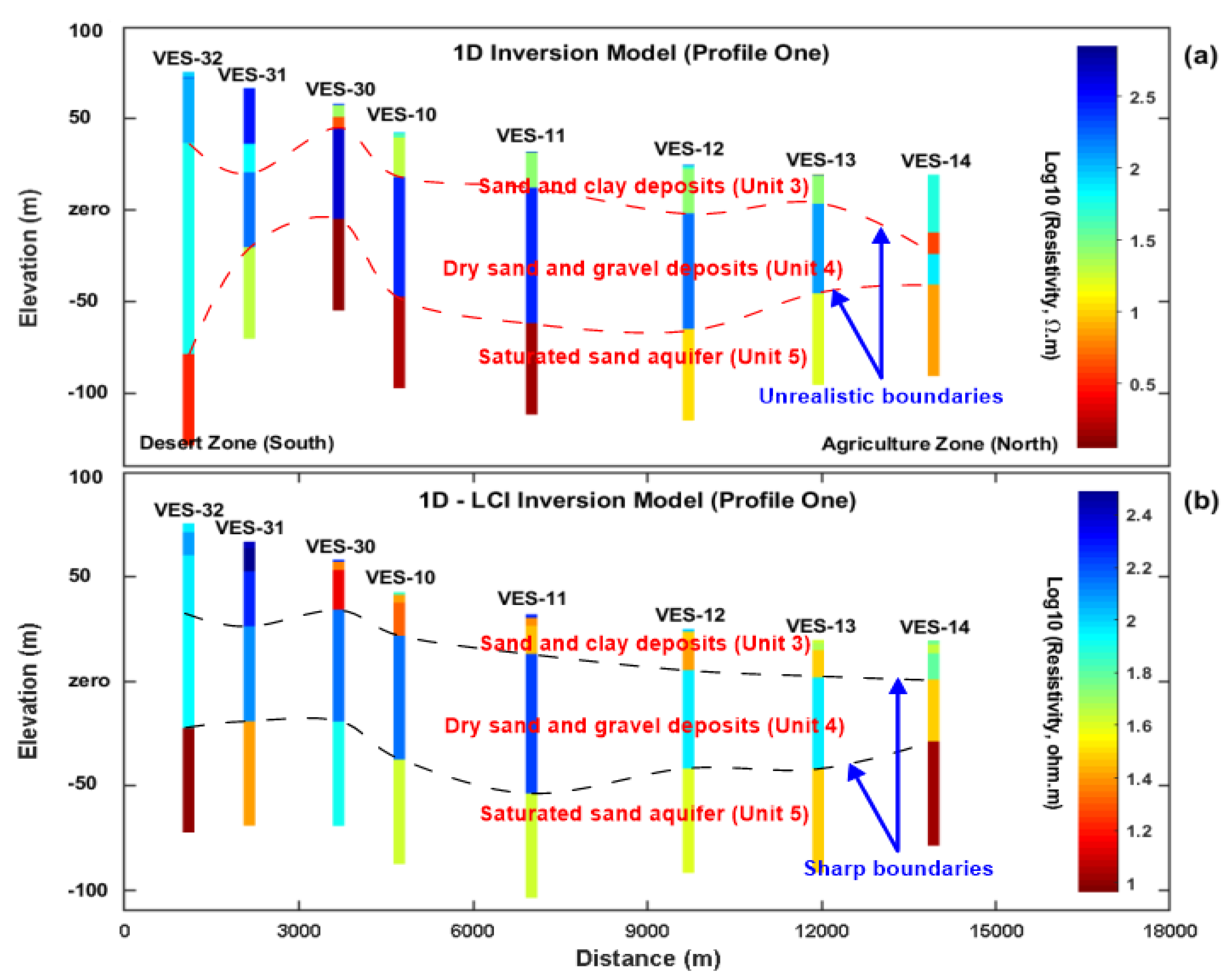
From the 1D inversion results, the indications of formation boundaries are seen, but they have a geologically unrealistic appearance (
Figure 7a) mainly because of equivalence problems [
45]. Also, the geometry of depth to top of the last layer and the thickness of a high resistive layer (forth layer) are not clear and poorly defined along all profiles. Therefore, we applied the 1D-LCI inversion on field data to solve this problem (
Figure 7b).
5.2. 1D-LCI Models
Five layers were used in the 1D-LCI section. The choice of this number of layers was based on three factors: the result from the conventional 1D inversion, the number of geological units in the generalized geological profile and the sensitivity analysis of model parameters in 1D-LCI. The 1D-LCI model clearly describes the horizontal layer interfaces of the different geological units. The constraints between resistivities and depth interfaces of neighboring VES sites, used in the 1D-LCI inversion along four profiles form a (0.3) factor.
Figure 8 and
Figure 9 show the laterally constrained (1D-LCI) inversion models of VES DC data along main profiles (a and c) and the analysis of model parameters (b and d). The lithologies of the main resistivity regime vary between surface clastic deposits, sandy clay, dry sand and gravel, and a saturated sand aquifer.
The models along all profiles contain five layers with smooth transitions in resistivities and layer boundaries, but the thin top layer is barely visible in this section. These models give a clear indication of a top variable resistive layer (40.4–257 Ωm), while still picking up the near surface resistivity changes overlying a second layer of high resistivity (11.5–486.3 Ωm), and a third layer of more resistivity (12.1–637 Ωm), underlain by a resistive layer (29.1–256.1 Ωm). A conductive layer is identified at the bottom with low resistivity values between (9.3–110 Ωm) along all profiles and a high resistivity value (237 Ωm) only below VES-24. This decrease of resistivity values emphasizes the effect of a shallow Quaternary groundwater aquifer in the saturated sand zone in the study area. The depth of this layer varies considerably along all the profiles from (34.5) m below VES-21 at the north to (118.4) m below VES-09 at the south.
The sensitivity analysis of the final models from 1D-LCI inversion results reveals well-determined model parameters in most parts of all the profiles, especially those concerning the resistivity parameter of five layers along profiles one, three and four (
Figure 8b and
Figure 9b,d, respectively), and the resistivity parameter of the first and second layer along profile two (
Figure 8d). However, the thickness of the fourth layer (Th.4) along all profiles, the thickness of the second layer (Th.2) along profiles one and three (
Figure 8b and
Figure 9b), and the thickness of the third layer (Th.3) along profiles three and four (
Figure 9b,d), are moderately resolved. In the 1D-LCI model, the upper boundary of the last conductive layer is sharp and well defined, and the thickness of its overlay are evident along the profile sections due to the constraints. So, the 1D-LCI produces a laterally smooth model with sharp layer boundaries where it describes the horizontal interfaces of the different geological units. The data error for the 1D-LCI inversion at VES stations along profile two reveals a misfit generally up to 20%, while the one along the other profiles reveals a misfit generally between (8–10.8%).
Table 2 shows the values of model parameters (resistivity and thickness) resulting from the lateral constrained (1D-LCI) inversion along all profiles.
Figure 10 shows the observed and calculated apparent resistivities of 1D-LCI inversions for some selected VES sites along all profiles where a good fitting between the observed and model data were achieved.
5.3. Two-Dimensional (2D) Inversion Results of the DC Data
Where multi-electrode device was not available for the survey, the field setup is designed for 1D interpretation. Although the distances between the VES sites were too large and no overlap of the VES data of neighbouring VES sites could be realized, a 2D inversion of the same DC data along the main profiles were achieved using the algorithm of Uchida (1990) to interpret all these VES data by one conductivity model simultaneously. The basic theory and the detailed description for inverting (2D) Schlumberger data using the Uchida algorithm has been discussed by the following authors [
44]. The inversion problem is solved using damped non-linear least squares inversion or Marquardt’s method. A forward calculation is made at each VES by using the initial model which is assumed to be 30 Ωm homogeneous earth, and the topography is incorporated into the models.
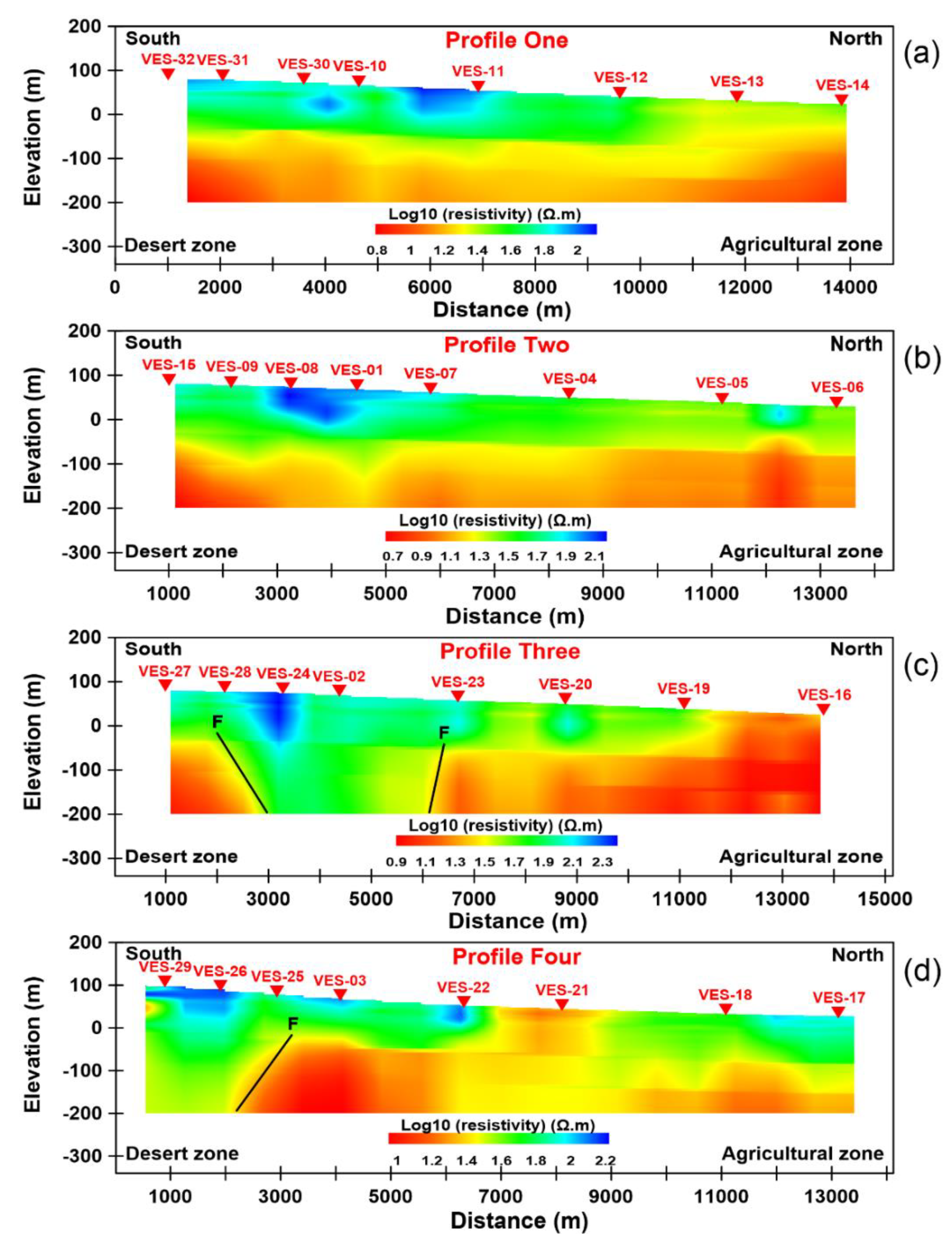
Figure 11 shows the cross sections of the two dimension (2D) inverted model from DC data along all profiles (a and b and c and d). The RMS misfit becomes nearly stable with minimum values equal to 0.2, after the second iteration along the four main profiles. The presence of different geo-electrical layers of variable resistivity values is mainly governed by the variation of lithology composed of alternations of gravel, sand and some clay of the Pleistocene deposits.
The correlation between 2D inverted cross-sections (
Figure 11), some spots of high resistive anomaly (300 Ωm) are characterized in their shallow zones, southern part of the study area. These spots represent the dry sand lenses and/or conglomerates of the Nile deposits that dominate in the desert zone, concerned below VES-11 and VES-31 and between VES-30 and VES-10 (profile one,
Figure 11a), below VES-08 and VES-01 and between them (profile two,
Figure 11b), below VES-24 (profile three,
Figure 11c), below VES-03 and VES-22 and between VES-29 and VES-26 (profile four,
Figure 11d). These inverted sections show that the lower layer of decreasing resistivity values reaches up 5 Ωm at 100 m depth that may reflect shallow Quaternary groundwater-bearing formation in the study area. A lateral change in resistivity in the shallow part of these sections from the south (arid desert zone) toward the north (moisture agriculture zone) is noticed due to the infiltration effect of El-Shabab Canal (north-east) and Ismailia Canal (north-west), and the presence of some clay lenses. Also, the senses of normal faulting are expected below the VES-28 and VES-24 along profile three and below VES-25 along profile four are observed trending generally E-W. Such interpreted faults agree well with the previous studies [
4] (
Figure 2).
Figure 12 shows the observed and calculated apparent resistivities of 2D inversions for some selected VES sites along all profiles where a good fitting between the observed and model data were achieved.
5.4. The Resistivity and Top Depth to Aquifer Layer
The spatial variation of the resistivity of the Quaternary groundwater aquifer derived by the 1D-LCI inversion of all VES sites on the four profiles of the study area is displayed in
Figure 13a. In addition, the spatial variation depth of the groundwater aquifer from this inversion is displayed in
Figure 13b. According to the 1D-LCI inversion results, the resistivity values range from (9.3 to 110 Ωm) in the study area. These values are high in the central part of the map, especially below VES-24 (237 Ωm), which may be related to the collection of some dry sand and conglomerates below these VES sites in the aquifer zone. The resistivity values decrease in the other part of the map (
Figure 13a). This decreasing resistivity values may result from the high salinity of the groundwater and from the effect of oxidation ponds and infiltration of wastewater from industries in Tenth of Ramadan City. The recharge of fresh water from the Ismailia Canal is the main reason for the resistivity decrement beneath the Quaternary deposits. The depth to the top saturated zone aquifer in the study area varies from 34.5 m to 118.4 m. This depth increases in the central and southern parts (high topography) of the map, especially below VES-04, VES-09 and VES-15, while it begins to decrease towards the north (low topography), towards the Ismailia Canal in the northwest direction, to the northeast and to the east (
Figure 13b). Finally, these results cope with the information from the boreholes (Well-P2 and P3-Well).
6. Discussion
The eastern Nile Delta in Egypt has recently become one of the most promising areas for various developments such as land reclamation for agriculture and new residential areas. The groundwater reserve in this area could be used as a potential source for irrigational and industrial purposes.
Revision of the previous geophysical work in the study area, mainly 1D inversion of DC resistivity, showed that the subsurface formation boundaries have sometimes geologically unrealistic appearance due to the equivalence problems. Therefore, we applied the 1D-LCI inversion of the DC resistivity data to solve the problem of inherent ambiguity and model equivalence.
In this work, the model parameters of poorly resolved individual data sets could be well resolved through the spreading of the constraint information from one model to the neighboring models. The lateral reference constrains of (0.3) proved to be best for identification of resistivities and thicknesses of the subsurface layers. From 1D-LCI inversion for some selected VES sites, a good fitting between the observed and model data were achieved. The final models from 1D-LCI inversion results reveal well-determined model parameters in most parts of all the profiles, especially those concerning the resistivities of the five layers well identified along all profiles with smooth boundaries. However, the thicknesses of these layers are moderately resolved. So, the 1D-LCI offers a good analysis of the model parameters, which was successfully used to characterize a zone of groundwater aquifer. There is good agreement between the 1D-LCI inversion models and the information from the nearest boreholes of P2-well and P3-well where the depth of the shallow aquifer begins at (80 m) depth. The resistivity of such a bearing water layer ranges between 9.3 and 110 Ωm and depth vary between 34.5 m 118.4 m with average depth approximately equal to 77.5 m in the area of study. The low resistivity in some zones within this aquifer, could be attributed to groundwater polluted irrigation drains, especially zones of thin or no clay cap.
It is generally shown that the depth topography of the water bearing zone is relatively related to the surface topography, and the general flow of groundwater is in the northerly direction. That depth ranges between 34.5 m and 118.4 m along the four main profiles in the area of study. The irregularity of the boundary surface along profile four, especially below VES-25 (
Figure 9c), may be related to the fault effect which is clearly identified on the 2D inversion results (
Figure 11d).
From the previous literature reviews, the area is affected by some normal faults. However, the 1D-LCI inversion failed to show the effects of the faults, as the 1D-LCI inversion technique is focused on the lateral smoothing of the models and produces sharp layer boundaries. Therefore, the 2D inversion results of the DC data have been considered to fill this gap below VES-23 and VES-28 along profile three (
Figure 11c), and VES-25 along profile four (
Figure 11d).
The 2D inverted models reflect generally three main layers which include a high resistive surface layer, relatively high resistive intermediate layer and low resistive layer (5 Ωm) at the deeper part of the sections. The later layer may reflect the saturated zone of groundwater aquifer at depth that reaches up to 100 m. This gives a good agreement between the 2D inverted models and the information from the nearest boreholes of P2-well and P3-well.
7. Conclusions
The present work aimed to delineate the shallow Quaternary groundwater aquifer in the study area. The 1D-LCI inversion is applied to VES DC resistivity data which are measured at 32 VES sites in the study area by using a Schlumberger array.
A general overview of the calculated 1D and 1D-LCI models from VES curves reveals five layers interpreted geo-electric layers along four long profiles. The 1D-LCI produces a laterally smooth model with sharp layer boundaries which describes the horizontal interfaces of the different geological units. The lithologies of the main resistivity regime vary between surface clastic deposits (high-resistive layer), sand with some clay (moderately resistive layer), dry sand and gravel (high-resistive layer), and saturated sand aquifer (conductive layer), respectively.
Results of the 1D-LCI inversion showed that the resistivity values of the last layer vary between (9.3 and 110 Ωm) and the depth to the top ranges between (34.5 and 118.4 m), and reflect a shallow Quaternary groundwater aquifer in the study area. However, the high resistivity value below VES-24 at profile three (237 Ωm) may reflect dry sand and gravel intercalation. The average depth to the top of the shallow groundwater aquifer in the study area approximately equals 77.5 m based on the 1D-LCI results agree well with the nearest boreholes of P2-well and P3-well (aquifer begins at 80 m depth).
The 2D inverted model reflects generally three main layers which include a high resistive surface layer that reaches up to 300 Ωm, relatively high resistive intermediate layer, and low resistive layer reaching up to 5 Ωm at the deeper part of the sections. The later layer may reflect the saturated zone of groundwater aquifer at depth reach up to 100 m. This gives a good agreement between the 2D inverted models and the information from the nearest boreholes of P2-well and P3-well. Some resistive spots in the shallow parts represent dry sand lenses and conglomerates of the Nile deposits that dominate in the desert zone.
Furthermore, the decrement of the resistivity value inside the aquifer may result from the high salinity of the groundwater or from the effect of oxidation ponds and the infiltration of wastewater from industries in Tenth of Ramadan City. The general decreases in the resistivity values from the south into the north direction in the shallow part of the interpreted sections are also due to infiltration from El Shabab canal (north-east) and Ismailia Canal (north-west), irrigation operated in the cultivated lowlands, and presence of some clay lenses. This average depth to the top of the shallow groundwater aquifer agrees well with these boreholes (aquifer begins at 80 m depth) while DC inversion results showed that the depth of the saturated groundwater aquifer reaches up to 100 and decreases towards Ismailia Canal in the north.
Some normal faults striking nearly E-W are interpreted in the southern part near Tenth of Ramadan City are observed from 2D inversion results that agree with the pervious known geology.
Finally, it is recommended that the applications of 1D-LCI in coordination with 2D inversion of DC data could successfully help to identify the groundwater aquifer and its extension. This result could help the stakeholders add new water wells in the newly reclaimed arid area. Other geophysical tools including magnetotelluric (MT) and electromagnetic (EM) are also recommended to identify the deeper groundwater aquifers (Miocene aquifer) and to clarify the interaction between the deep and shallow aquifer in the area of study.
Author Contributions
M.G. (conceptualization, data curation, methodology, software, writing-original draft preparation). H.G. (supervision, conceptualization, data curation, writing-review and editing). A.M. (supervision, conceptualization). U.M. (supervision, conceptualization). B.T. (supervision, methodology, software, data curation, writing-review and editing). All authors have read and agreed to the published version of the manuscript.
Data Availability Statement
Selective Examples of the data is contained within the article.
Acknowledgments
We are indebted to the Hydro-geophysics Group of the University of Aarhus, Denmark, for their useful help us in giving the inversion code (AarhusInv software) for a 1D-LCI constrained inversion. Also, I would like to thank the Institute of Geophysics and Meteorology at the University of Cologne, Germany, for hosting me for two years as a member of an Egyptian-German joint supervision mission and for paying the cost of publishing this article.
Conflicts of Interest
The authors declare no conflict of interest. The funder has a role in the analyses and interpretation of data, in the writing of the manuscript and in the decision to publish the results.
References
- Hashemi, M.; Zadeh, H.M.; Arasteh, P.D.; Zarghami, M. Economic and environmental impacts of cropping pattern elements using systems dynamics. Civ. Eng. J. 2019, 5, 1020–1032. [Google Scholar] [CrossRef] [Green Version]
- Taha, A.A.; El-Mahmoudi, A.S.; El-Haddad, I.M. Pollution sources and related environmental impacts in the new communities southeast Nile Delta, Egypt. Emir. J. Eng. Res. 2004, 9, 35–49. [Google Scholar]
- Abo El-Fadl, M.M. Possibilities of groundwater pollution in some areas, East of Nile Delta, Egypt. Hydrogeochemistry Department, Desert Research center, El-Matariya, Cairo, P.O.B 11753, Egypt. Int. J. Environ. 2013, 1, 1–21. [Google Scholar]
- El-Fayoumi, I.F. Geology of the Groundwater Supplies in the Eastern Region of the Nile Delta and Its Extension in the North Sinai. PhD Thesis, Cairo University, Giza, Egypt, 1968; 207p. [Google Scholar]
- Reynolds, J.M. An Introduction to Applied and Environmental Geophysics; John Wiley & Sons: Hoboken, NJ, USA, 2011. [Google Scholar]
- Keller, G.V.; Frischknecht, F.C. Electrical Methods in Geophysical Prospecting; Pergamon Press: New York, NY, USA, 1966; 517p. [Google Scholar]
- Zohdy, A.A.R. Electrical Methods Application of Surface Geophysics to Groundwater Investigation. In Techniques of Water Resources Investigations of the United States Geological Survey (USGS); USGS: Reston, VA, USA, 1974; 66p. [Google Scholar]
- Auken, E.; Christiansen, A.V.; Jacobsen, B.H.; Foged, N.; Sørensen, K.I. Piecewise 1D laterally constrained inversion of resistivity data. Geophys. Prospect. 2005, 53, 497–506. [Google Scholar] [CrossRef]
- Christiansen, A.V.; Auken, E.; Foged, N.; Sørensen, K.I. Mutually and laterally constrained inversion of CVES and TEM data: A case study. Near Surf. Geophys. 2007, 5, 115–123. [Google Scholar] [CrossRef] [Green Version]
- Steuer, A. Joint Application of Ground-Based Transient Electromagnetics and Airborne Electromagnetics. Ph.D. Thesis, Universität zu Köln, Köln, Germany, 2008; 125p. [Google Scholar] [CrossRef]
- Auken, E.; Christiansen, A.V. Layered and laterally constrained 2D inversion of resistivity data. Geophysics 2004, 69, 752–761. [Google Scholar] [CrossRef]
- Wisén, R.; Auken, E.; Dahlin, T. Combination of 1D laterally constrained inversion and 2D smooth inversion of resistivity data with a priori data from boreholes. Near Surf. Geophys. 2005, 3, 71–79. [Google Scholar] [CrossRef] [Green Version]
- Auken, E.; Foged, N.; Sørensen, K.I. Model recognition by 1-D laterally constrained inversion of resistivity data. In Proceedings of the 8th EEGS-ES Meeting, Aveiro, Portugal, 8–12 September 2002; pp. 241–244. [Google Scholar] [CrossRef]
- Küpper, M. Transient Electromagnetic Measurements Using a Floating Setup on the Volcanic Lake Lagoa das Furnas, São Miguel, Azores. Master’s Thesis, University of Cologne, Cologne, Germany, 2018. [Google Scholar]
- Lin, C.; Fiandaca, G.; Auken, E.; Couto, M.A.; Christiansen, A.V. A discussion of 2D induced polarization effects in airborne electromagnetic and inversion with a robust 1D laterally constrained inversion scheme. Geophysics 2019, 84, E75–E88. [Google Scholar] [CrossRef]
- Melo, D.C.; Régis, C.R.T. 1D laterally constrained inversion of 2D MT data. In Proceedings of the 15th International Congress of the Brazilian Geophysical Society & EXPOGEF, Rio de Janeiro, Brazil, 31 July–3 August 2017; pp. 154–159. [Google Scholar] [CrossRef]
- Schmalz, T.; Tezkan, B. 1D-Laterally Constraint Inversion (1D-LCI) of Radiomagnetotelluric Data from a Test Site in Denmark. In Kolloquium Elektromagnetische Tiefenforschung; Hotel Maxičky: Děčín, Czech Republic, 2007. [Google Scholar]
- Shlykov, A.; Saraev, A.; Agrahari, S.; Tezkan, B.; Singh, A. One-dimensional Laterally Constrained Joint Anisotropic Inversion of CSRMT and ERT Data. J. Environ. Eng. Geophys. 2021, 26, 35–48. [Google Scholar] [CrossRef]
- Ourania, P. Laterally Constrained Inversion of Electrical Resistivity Tomography Data. Master’s Thesis, Aristotle University of Thessaloniki, Thessaloniki, Greek, 2021. [Google Scholar]
- Pelton, W.H.; Rijo, L.; Swift, C.M., Jr. Inversion of two-dimensional resistivity and induced-polarization data. Geophysics 1978, 43, 788–803. [Google Scholar] [CrossRef]
- Sasaki, Y. Two-dimensional joint inversion of magnetotelluric and dipole-dipole resistivity data. Geophysocs 1989, 54, 254–262. [Google Scholar] [CrossRef]
- Tripp, A.C.; Homann, G.W.; Swift, C.M., Jr. Two-domensional resistivity inversion. Geophysics 1984, 49, 1708–1717. [Google Scholar] [CrossRef]
- Attwa, M.; Gemail, K.; Eleraki, M.; Zamzam, S. Assessment of oxidation ponds impact using DC resistivity method in Tenth of Ramadan city, Egypt. In Proceedings of the 20th international geophysical congress and exhibition of Turkeyi, Antalya, Turkeyi, 25–27 November 2013; pp. 25–27. [Google Scholar] [CrossRef]
- Attwa, M.; Gemail, K.; Eleraki, M.; Zamzam, S. Application of genetic algorithm (GA) for soil characterization using DC resistivity data: A case study in Tenth of Ramadan city, Egypt. Adv. Nat. Appl. Sci. 2014, 8, 38–50. [Google Scholar]
- Massoud, U.; Khalil, M.M.; Tokunaga, T.; Santos, F.A. Preliminary hydrogeophysical investigation at the 10th of Ramadan City, Egypt, by 1D and 2D inversion of VES data. Near Surf. Geophys. 2016, 14, 287–297. [Google Scholar] [CrossRef]
- El-Shazly, E.M.; Abdel Hady, M.A.; El-Shazly, M.M.; El-Ghawabby, M.A.; El-Kassa, I.A.; Salman, A.E.; Morsi, M.A. Geological and Groundwater Potential Studies of El Ismailia Master Plan Study Area “Remote Sensing Research Project; Academy of Scientific Research and Technology: Cairo, Egypt, 1975; pp. 1–24. [Google Scholar]
- FAO (Food and Agriculture Organization of the United Nations). High Dam Soil Survey Project; Food and Agriculture Organization of the United Nations (FAO), Ministry of Agric: Cairo, Egypt, 1966; Volume 3, pp. 1–348. [Google Scholar]
- Hefny, K.; Farid, M.S.; Morsi, A.; Khater, A.R.; El-Ridi, M.R.; Khalil, Z.B.; Atwa, A.; Attia, D. Groundwater Studies for the Tenth of Ramadan City; Unpublished internal rept; Research Institute for Groundwater, Ministry of Public works and Water Researches: Cairo, Egypt, 1980; 54p. [Google Scholar]
- RIGW–IWACO. Environmental Management of Groundwater Resources (EMGR): Identification, Priority Setting and Selection of Area for Monitoring Groundwater Quality; Technical Report TN/70.00067/WQM/97/20; Research Institute For Groundwater (RIGW), National Water Research Center: El Kanter El Khairia, Egypt, 1998. [Google Scholar]
- El-Arabi, N. Environmental impact of new settlements in Egypt. In Groundwater in the Urban Environment; August Aimé Balkema: Nottingham, UK, 1997; Volume 1, pp. 285–290. [Google Scholar]
- Ibrahim, L.A.; Nofal, E.R. Quality and hydrogeochemistry appraisal for groundwater in Tenth of Ramadan Area, Egypt. Water Sci. 2020, 34, 50–64. [Google Scholar] [CrossRef] [Green Version]
- El-Haddad, I.M. Groundwater Sources and Soil Evaluation for the Tenth of Ramadan City Area and its Surroundings, Egypt. Master’s Thesis, Mansoura University, Mansoura, Egypt, 1996; 199p. [Google Scholar]
- Al shahat, F.M.; Sadek, M.A.; Mostafa, W.M.; Hagagg, K. Hydrogeochemical indicators for radioactive waste disposal site survey to the east of Nile Delta, Egypt. Int. J. Curr. Eng. Technol. 2014, 4, 549–556. Available online: http://inpressco.com/category/ijcet (accessed on 5 June 2021).
- Khater, A.R. Evaluation of the Current Practice of Groundwater Monitoring and Protection in Egypt; ACSAD-BGR Technical Cooperation Project; Arab Centre for the Study of Arid and Dry Lands (ACSAD): Damascus, Syria, 2002. [Google Scholar]
- Christiannen, A.V.; Auken, E.; Sorensen, K.I.; Jorgensen, F.; Johnsen, R. From resistivity to geophysical clay thickness—An inversion approach. In Proceedings of the XVI International Conference on Computational Methods in Water Resources (CMWR-XVI), Copenhagen, Denmark, 18–22 June 2006. [Google Scholar]
- Eleraki, M.; Gadallah, M.; Gemail, K.; Attwa, M. Application of resistivity method in environmental study of the appearance of soil water in the central part of Tenth of Ramadan City, Egypt. Q. J. Eng. Geol. Hydrogeol. 2010, 43, 171–184. [Google Scholar] [CrossRef]
- Isaaks, E.H.; Srivastava, R.M. An Introduction to Applied Geostatistics; Oxford University Press, Inc.: New York, NY, USA, 1989. [Google Scholar]
- Johansen, H.K. A man/computer interpretation system for resistivity soundings over a horizontally stratified earth. Geophys. Prospect. 1977, 25, 667–691. [Google Scholar] [CrossRef]
- Ward, S.H.; Hohmann, G.W. Electromagnetic theory for geophysical applications. In Electromagnetic Methods in Applied Geophysics; Nabighia, M.N., Ed.; Society of Exploration Geophysicists: Tulsa, OK, USA, 1988; Volume 1, 531p. [Google Scholar] [CrossRef]
- Menke, W. Geophysical Data Analysis: Discrete Inverse Theory; Academic Press Inc.: Cambridge, MA, USA, 1989. [Google Scholar]
- Tarantola, A.; Valette, B. Generalized nonlinear inverse problems solved using a least squares criterion. Rev. Geophys. Space Phys. 1982, 20, 219–232. [Google Scholar] [CrossRef]
- Bobachhev, A.A.; Modin, I.N.; Shevnin, V.A. IPI2Win Program for Vertical Electrical Sounding Curves 1D Interpreting along a Single Profile. Ph.D. Thesis, Moscow University, Moscow, Russia, 2001. [Google Scholar]
- HGG. AarhusInv Manual; Hydrogeophysics Group, University of Aarhus: Aarhus, Denmark, 2012. [Google Scholar]
- Uchida, T.; Murakami, Y. Development of a Fortran Code for the Two-Dimensional Schlumberger Inversion; Geological survey of Japan open-file report No.150; Geological Survey of Japan: Tsukuba City, Japan, 1990; 19p. [Google Scholar]
- Genedi, M.A.; Ghazala, H.; Mohamed, A.K.; Massoud, U. Joint inversion of DC/TDEM data: A Case study of Static Shift problem in the area north Tenth of Ramadan City, Egypt. Arab. J. Geosci. 2021. submitted. [Google Scholar]
Figure 1.
(a) Google map of Egypt, (b) Surface geological map of the study area and the location of the vertical electrical sounding (VES) stations along four main profiles, and (c,d) lithostratigraphic column of nearby boreholes from the study area (P2-Well and P3-Well).
Figure 1.
(a) Google map of Egypt, (b) Surface geological map of the study area and the location of the vertical electrical sounding (VES) stations along four main profiles, and (c,d) lithostratigraphic column of nearby boreholes from the study area (P2-Well and P3-Well).
Figure 2.
Structural zones of the eastern Nile Delta and area of study (modified after El-Fayoumi, 1968 [
4]).
Figure 2.
Structural zones of the eastern Nile Delta and area of study (modified after El-Fayoumi, 1968 [
4]).
Figure 3.
(a) Location map of VES sites on the agriculture zone in the north half of the study area and on the desert zone in the southern half of the study area, and (b) apparent resistivity as function of electrode distances (AB/2) of some selected VES data along four main profiles on the agriculture zone and on the desert zone.
Figure 4.
Apparent resistivity maps for different (AB/2) values in the study area. (a) AB/2 = 3 m; (b) AB/2 = 10 m; (c) AB/2 = 40 m; (d) AB/2 = 100 m; (e) AB/2 = 400 m; (f) AB/2 = 500 m.
Figure 4.
Apparent resistivity maps for different (AB/2) values in the study area. (a) AB/2 = 3 m; (b) AB/2 = 10 m; (c) AB/2 = 40 m; (d) AB/2 = 100 m; (e) AB/2 = 400 m; (f) AB/2 = 500 m.
Figure 5.
Flowchart of the Aaarhus algorithm.
Figure 5.
Flowchart of the Aaarhus algorithm.
Figure 6.
(
a,
c) Observed and calculated apparent resistivities as a function of electrode distances (AB/2) for the VES-10 and VES-25, (
b,
d) 1D inversion models of the observed apparent resistivities of the VES-10 and VES-25, and its comparison with the nearest boreholes (P2 and P3 Wells, respectively,
Figure 1c,d).
Figure 7.
Inversion result from conventional 1D inversion model (a) and synchronized 1D–LCI inversion model (b) using five layers, constructed from VES soundings along profile one.
Figure 7.
Inversion result from conventional 1D inversion model (a) and synchronized 1D–LCI inversion model (b) using five layers, constructed from VES soundings along profile one.
Figure 8.
(a,c) Inversion result from synchronized 1D–LCI inversion model using five layers, constructed from DC VES soundings along profiles one and two, respectively. (b,d) Detailed plot of the solution analysis of model parameters, calculated from final model of 1D– LCI inversion (resistivities; Res.1–Res.5 and thicknesses; Th.1–Th.4) along profiles one and two, respectively. The color-coding of the analysis ranging from red (well resolved parameter, STD factor = 1) to blue (moderately resolved parameter, STD Factor = 1.2).
Figure 9.
(a,c) Inversion result from synchronized 1D–LCI inversion model using five layers, constructed from DC soundings along profile three and four, respectively. (b,d) Detailed plot of the resolution analysis of model parameters calculated from final model of 1D–LCI inversion (resistivities; Res.1–Res.5 and thicknesses; Th.1–Th.4) along profiles three and four, respectively. The color-coding of the analysis ranging from red (well resolved parameter, STD factor = 1) to blue (moderately resolved parameter, STD Factor = 1.2).
Figure 10.
Comparison of the observed and 1D-LCI synthetic data of some selected VES sites such as VES-12 (a), VES-01 (b), VES-19 (c), and VES-17 (d) along all the profiles.
Figure 10.
Comparison of the observed and 1D-LCI synthetic data of some selected VES sites such as VES-12 (a), VES-01 (b), VES-19 (c), and VES-17 (d) along all the profiles.
Figure 11.
Two-dimensional (2D) inversion models of VES sites along four main profiles. The “F” symbol indicates the fault. (a) Profile One; (b) Profile Two; (c) Profile Three; (d) Profile Four.
Figure 11.
Two-dimensional (2D) inversion models of VES sites along four main profiles. The “F” symbol indicates the fault. (a) Profile One; (b) Profile Two; (c) Profile Three; (d) Profile Four.
Figure 12.
Comparison of the observed and 2D synthetic data of some selected VES sites along all profiles.
Figure 12.
Comparison of the observed and 2D synthetic data of some selected VES sites along all profiles.
Figure 13.
(a) Image map of true resistivity values from 1D-LCI inversion results in the study area and (b) image map of depth to top saturated zone of ground water aquifer from 1D-LCI inversion results in the study area.
Figure 13.
(a) Image map of true resistivity values from 1D-LCI inversion results in the study area and (b) image map of depth to top saturated zone of ground water aquifer from 1D-LCI inversion results in the study area.
Table 1.
Example of raw electrical resistivity (DC) data (apparent resistivity and AB/2) at some selected VES stations along the main profiles.
Table 1.
Example of raw electrical resistivity (DC) data (apparent resistivity and AB/2) at some selected VES stations along the main profiles.
| Stations | VES-01 | VES-12 | VES-17 | VES-19 |
|---|
| AB/2 (m) | Apparent Resistivity (Ωm) |
|---|
| 1 | 145.5 | 96 | 373.3 | 198 |
| 1.4 | 130.7 | 86.2 | 365.5 | 163.8 |
| 2 | 102.4 | 65.7 | 405.6 | 146.1 |
| 3 | 67.8 | 49.6 | 317.7 | 133.6 |
| 4 | 45.7 | 40.3 | 202.4 | 114.4 |
| 3 | 81.9 | 54.4 | 220 | 142.2 |
| 4 | 55.8 | 43.6 | 141.3 | 121.3 |
| 6 | 39.5 | 36.9 | 120.4 | 80.5 |
| 8 | 32.5 | 30.2 | 80.8 | 57 |
| 10 | 30.3 | 27.6 | 62 | 43.7 |
| 14 | 29.8 | 26.9 | 61.2 | 30.6 |
| 10 | 30.9 | 29.2 | 72.7 | 52.7 |
| 14 | 29.9 | 28.3 | 67.5 | 35.6 |
| 20 | 32.5 | 29.9 | 68.1 | 36.1 |
| 30 | 40.5 | 33.9 | 73.9 | 44.8 |
| 40 | 41.4 | 39.1 | 66.9 | 52.4 |
| 30 | 36.9 | 29.7 | 46.6 | 40.3 |
| 40 | 37.9 | 34.3 | 42.6 | 46.3 |
| 60 | 48.8 | 42.7 | 44.8 | 56.8 |
| 80 | 61.3 | 45.8 | 45.7 | 58.1 |
| 100 | 71.4 | 50.1 | 44 | 57.4 |
| 140 | 77.4 | 58.6 | 43.1 | 52.8 |
| 100 | 64.7 | 55.3 | 43.1 | 56.6 |
| 140 | 70.8 | 60.9 | 42.6 | 50.7 |
| 200 | 76.7 | 46.8 | 36.9 | 36.7 |
| 300 | 57.8 | 49.4 | 30.8 | 19.7 |
| 400 | 91.8 | 33 | 23.8 | 13.1 |
| 500 | 201 | 10.6 | 17.5 | 4 |
Table 2.
The range of the parameters values (resistivity and thickness) resulted from 1D-LCI inversion models along the main profiles.
Table 2.
The range of the parameters values (resistivity and thickness) resulted from 1D-LCI inversion models along the main profiles.
| Profiles | Layer Number | Resistivity (Ωm) | Thickness (m) | Depth of Last Layer (m) |
|---|
| Profile One | Layer one | (40.4–257) | (1.04–4.32) | |
| Layer two | (22.5–316) | (3.48–11.1) |
| Layer three | (13.6–183) | (12.5–28.7) |
| Layer four | (29.1–169) | (29.6–66.8) |
| Layer five | (9.3–79.7) | | (48.3–98) |
| Profile Two | Layer one | (63.7–171) | (1.3–2.54) | |
| Layer two | (23.8–418) | (7.78–13.9) |
| Layer three | (54.1–637) | (28.7–57.2) |
| Layer four | (61.8–143) | (43.9–65.5) |
| Layer five | (9.6–110) | | (89.7–118.4) |
| Profile Three | Layer one | (54.4–246) | (0.79–2.53) | |
| Layer two | (11.5–143) | (3.72–6.86) |
| Layer three | (29.8–481) | (14.3–31.7) |
| Layer four | (51.2–241) | (19.5–69.7) |
| Layer five | (11.3–237) | | (38.3–108.5) |
| Profile Four | Layer one | (14.9–388) | (066–2.92) | |
| Layer two | (27.08–486.3) | (1.83–6.05) |
| Layer three | (12.08–147.1) | (7.98–16.39) |
| Layer four | (71.48–256.1) | (17.2–59.24) |
| Layer five | (12.79–93.32) | | (34.5–82.6) |
| Publisher’s Note: MDPI stays neutral with regard to jurisdictional claims in published maps and institutional affiliations. |
© 2021 by the authors. Licensee MDPI, Basel, Switzerland. This article is an open access article distributed under the terms and conditions of the Creative Commons Attribution (CC BY) license (https://creativecommons.org/licenses/by/4.0/).


