Quasi-Linear Model of Tsunami Run-Up on a Beach with a Seafloor Described by the Piecewise Continuous Function

Abstract

The purpose of this paper is to propose the quasi-linear theory of tsunami run-up and run-down on a beach with complex bottom topography. We begin with the one-dimensional nonlinear shallow-water wave equations, which we consider over a beach of complex geometry that can be modeled by a piecewise continuous function, along with several natural initial and boundary conditions. The primary obstacle in solving this problem is the moving boundary associated with the shoreline motion. To avoid this difficulty, we replace the moving boundary with a stationary boundary by applying a transformation to the spatial variable of the computational domain. A characteristic feature of any tsunami problem is the smallness of the parameter $\epsilon ={\eta }_0/h_0$, where ${\eta }_0$ is the characteristic amplitude of the wave, and $h_0$ is the characteristic depth of the ocean. The presence of this small parameter enables us to effectively linearize the problem by using the method of perturbations, which leads to an analytical solution via an integral transformation. This analytical solution assumes that there is no wave breaking. In light of this assumption, we introduce the wave no-breaking criterion and determine bounds for the applicability of our theory. The proposed model can be readily used to investigate the tsunami run-up and draw-down for different sea bottom profiles. The novel particular solution, when the seafloor is described by the piecewise linear function, is obtained, and the effects of the different beach profiles and initial wave locations are considered.

1. Introduction

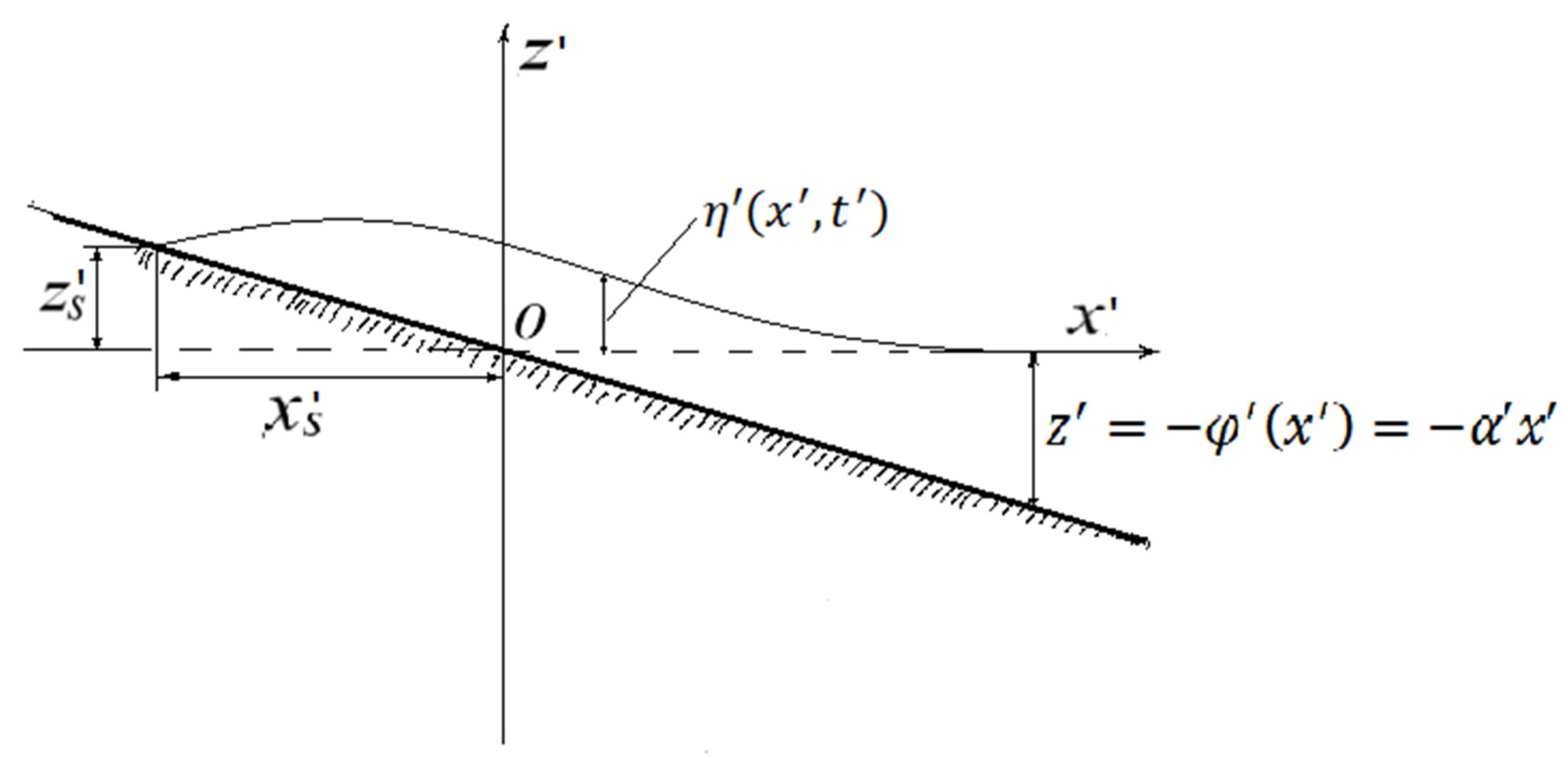
A characteristic feature of the propagation of long waves in the ocean is the smallness of the parameter δ = h₀/λ, where h₀ is the characteristic depth of the ocean, and λ is the characteristic wavelength (for example, this may be the case when h₀ = 4 km and λ = 100 km, and, therefore, δ ≈ 0.04 ≪ 1). This fact allows us to simulate the long-wave run to the shore of a reservoir, using shallow water equations [1]. A complete derivation of the shallow water equations from the more general Navier–Stokes equations is given in [2]. The first analytical solution of the tsunami break-in on an inclined beach was obtained in a rather complicated paper by Carrier and Greenspan [3]. Relatively recent advances in analytical approaches to the long-wave run problem are presented in [4,5,6,7], where some exact analytical solutions were obtained for the specific geometry of a sloping beach. Didenkulova and Pelinovsky [8] considered situations when the wave run-up takes place without wave reflection. This effect occurs when the seafloor geometry can be approximated by the function of the order of x^4/3. In their recent work, Rybkin et al. [9,10] generalized the Carrier and Greenspan [3] hodograph transform approach and applied it to the flow in the U-shape channel. As a result, several particular analytical solutions were obtained. Chugunov et al. [11] effectively applied the approximate approach for solving exactly the same problem, with the same seafloor geometry as used in [3,4] (see Figure 1). In [11], it was shown that the approximate method works well and, therefore, can be potentially applied to the problems with more complex seafloor topography.

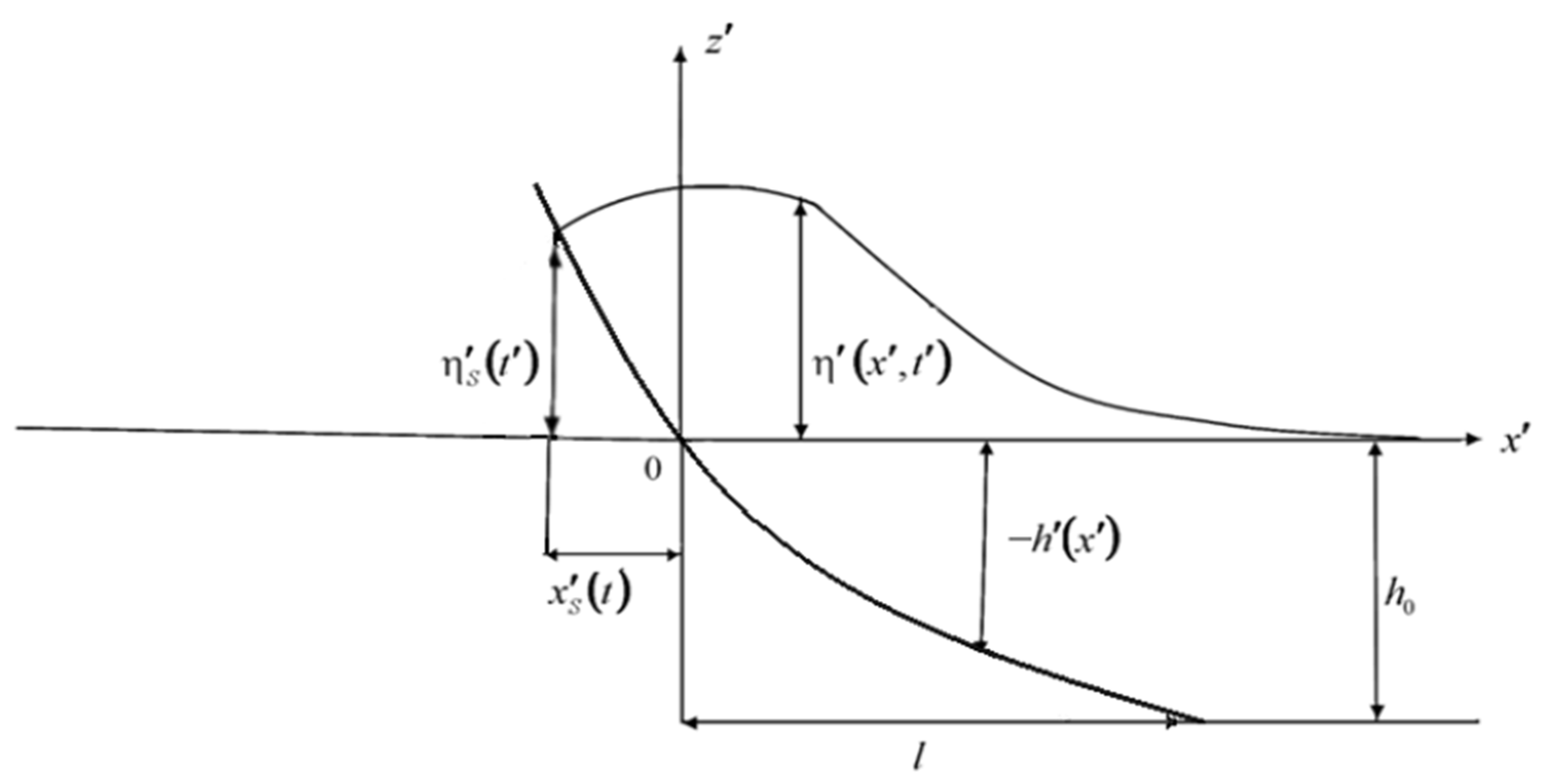
In our present work, we extend the approach suggested in [11] and formulate the mathematical model of tsunami dynamics for the seafloor that has an inclined curvilinear (or linear) portion near the shore and a horizontal section which models the seafloor at the certain distance from the shore (see Figure 2). We derive a quasilinear model of tsunami run-up on the beach of this complex topography and demonstrate the applicability of this quasilinear model to the more complex configuration of the beach shape than was discussed in [3,4,11]. Using as an example the seafloor profile that can be described by a piecewise linear function (with inclined and horizontal sections), we obtain the novel analytical solution and demonstrate the efficiency of the suggested approach for solving the problem analytically in the case of the complex seafloor topography.

2. System Model

As discussed above, we begin with the nonlinear shallow-water wave equations, which can be found in [1,2,3,11,12]:

$$\frac{\partial u^{\prime }}{\partial t^{\prime }}+u^{\prime }\frac{\partial u^{\prime }}{\partial x^{\prime }}+g\frac{\partial {\eta }^{\prime }}{\partial x^{\prime }}=0$$

(1)

$$\frac{\partial {\eta }^{\prime }}{\partial t^{\prime }}+\frac{\partial \left(\left[{\eta }^{\prime }+{\phi }^{\prime }\left(x^{\prime }\right)\right]u^{\prime }\right)}{\partial x^{\prime }}=0.$$

(2)

The relevant variables in our equations are as follows:

• ${\eta }^{\prime }$—the wave profile, measured as displacement from still-water level;
• $u^{\prime }$—the horizontal depth-averaged velocity;
• $t^{\prime }$—time;
• $x^{\prime }$—spatial variable;
• $l$—location of the sharp change of the water bed profile;
• $g$—gravity acceleration;
• $x_s^{\prime }\left(t\right)$—location of the water-soil interface (the time-dependent distance from the shoreline to the point where the total depth of the water vanishes);
• $z^{\prime }=-{\phi }^{\prime }\left(x^{\prime }\right)$—function that describes the seafloor geometry.

Note that the ‘prime’ notation used here refers to a dimensional variable, which has a unit of measurement attached, not a derivative.

We define the following:

$${\eta }_s^{\prime }\left(t\right)={\eta }^{\prime }\left(-x_s^{\prime }\left(t^{\prime }\right),t^{\prime }\right)$$

(3)

For the case presented in Figure 2, the seafloor can be defined by the arbitrary piecewise smooth function, where

$$z^{\prime }=-{\phi }^{\prime }\left(x^{\prime }\right)=\left\{\begin{array}{c}{h}^{\prime }\left(x^{\prime }\right), x^{\prime }<l\\ h_0, x^{\prime }>l,\end{array}\right.$$

(4)

such that ${\left.\frac{\partial {\phi }^{\prime }\left(x^{\prime }\right)}{\partial x^{\prime }}\right|}_{x^{\prime }=0}\ne 0\left(\mathrm{or}\infty \right),\mathrm{but}{\phi }^{\prime }\left(0\right)=0,$ where $h^{\prime }\left(x^{\prime }\right)$ defines the shape of a beach.

Equations (1) and (2) should be solved with following initial conditions:

$$t^{\prime }=0, {\eta }_s^{\prime }\left(x^{\prime },0\right)=f^{\prime }\left(x^{\prime }\right);$$

(5)

$$u^{\prime }\left(x^{\prime },0\right)=0.$$

(6)

These conditions suggest that, at time $t^{\prime }=0$, the water is motionless, but some disturbance (typically an earthquake) has created an initial wave profile at some distance from the shoreline.

We now consider boundary conditions for $x^{\prime }\to \infty$. Assuming that in the domain far from the initial wave the water level is undisturbed, we can write the following:

$$\underset{x^{\prime }\to \infty }{\lim }{\eta }^{\prime }\left(x^{\prime },t^{\prime }\right)=0$$

(7)

$$\underset{x^{\prime }\to \infty }{\lim }{u}^{\prime }\left(x^{\prime },t^{\prime }\right)=0$$

(8)

There is also an obvious relationship on the moving boundary:

$$x^{\prime }=-x_s^{\prime }\left(t\right), {\eta }^{\prime }\left(-x_s^{\prime }\left(t^{\prime }\right), t^{\prime }\right)=-{\phi }^{\prime }\left(-x_s^{\prime }\right)$$

(9)

$$u^{\prime }\left(-x_s^{\prime }\left(t^{\prime }\right),t^{\prime }\right)=-\frac{d{x}_s^{\prime }\left(t^{\prime }\right)}{d{t}^{\prime }}$$

(10)

To begin the nondimensionalization process, we here introduce the following characteristic scales:

• $h_0$—characteristic depth of the ocean;
• $u_0$—characteristic horizontal water velocity;
• $c_0$—characteristic velocity of the wave;
• $t_0$—characteristic time;
• ${\eta }_0$—characteristic amplitude of the wave.

Using these scales, we replace our original variables with nondimensional variables:

$$x_s=\frac{x_s^{\prime }}{l}; t=\frac{t^{\prime }}{t_0}; u=\frac{u^{\prime }}{u_0}; x=\frac{x^{\prime }}{l}; \eta =\frac{{\eta }^{\prime }}{{\eta }_0}; \phi \left(x\right)=\frac{{\phi }^{\prime }\left(x^{\prime }\right)}{h_o}; h=\frac{h^{\prime }}{h_0}.$$

(11)

It must also be the case that

$$c_0{u}_0=g{\eta }_0$$

(12)

$${\eta }_0{c}_0=u_0{h}_0,$$

(13)

and, as a result of these correlations, we have

$$c_0=\sqrt{g{h}_0}\mathrm{and}{u}_0={\eta }_0\sqrt{\frac{g}{h_0}}.$$

(14)

Substituting our nondimensional variables into Equations (1) and (2), and accounting for the above correlations, we obtain nondimensionalized versions of the governing nonlinear shallow-water wave equations:

$$\frac{\partial u}{\partial t}+\epsilon u \frac{\partial u}{\partial x}+\frac{\partial \eta }{\partial x}=0,$$

(15)

$$\frac{\partial \eta }{\partial t}+\frac{\partial }{\partial x}\left[u\left(\phi \left(x\right)+\epsilon \eta \right)\right]=0,$$

(16)

where $\epsilon ={\eta }_0/h_0$. The initial conditions can be easily rewritten in terms of the new variables:

$$t=0, \eta \left(x,0\right)=f\left(x\right),$$

(17)

$$u\left(x,0\right)=0,$$

(18)

The boundary conditions will take the following form:

$$x=-x_s\left(t\right), \epsilon \eta \left(-x_s,t\right)=-\phi \left(-x_s\right),$$

(19)

$$\epsilon u\left(-x_s\left(t\right),t\right)=-\frac{d{x}_s}{dt}$$

(20)

$$x\to \infty , \underset{x\to \infty }{\lim }\eta \left(x,t\right)=\underset{x\to \infty }{\lim }u\left(x,t\right)=0$$

(21)

Function $z=-\phi \left(x\right)$, which describes the seafloor profile (4) in a nondimensional form, can be rewritten as follows:

$$\phi \left(x\right)=\left\{\begin{array}{c}h\left(x\right), x<1\\ 1, x\ge 1,\end{array}\right.$$

(22)

As a final note, we assume (in accordance with real-world intuition) that, in the vicinity of the point $x=0$, the derivative of $\phi$ exists, ${\left|\frac{d\phi }{dx}\right|}_{x=0}\ne 0 \left(\mathrm{or} \infty \right)$, and $\phi \left(0\right)=0$.

Expanding Equation (19) into a Taylor series, we see that $x_s$ is of the same order as the parameter $\epsilon$:

$$\epsilon \left(\eta \left(0,t\right)-{\left.\frac{\partial \eta }{\partial x}\right|}_{x=0}{x}_s+O\left(x_s^2\right)\right)={\left.\frac{\partial \phi }{\partial x}\right|}_{x=0}{x}_s+O\left(x_s^2\right),$$

or

$$\epsilon \eta \left(0,t\right)={\left.\left(\frac{d\phi }{dx}+\epsilon \frac{\partial \eta }{\partial x}\right)\right|}_{x=0}{x}_s+O\left(x_s^2\right).$$

(23)

The coefficient in front of $x_s$ on the right-hand side of Equation (23) is of the order $O\left(1\right)$, and therefore $x_s=O\left(\epsilon \right)$. Hence, if we define the new function $x_m=x_s/\epsilon$, then $x_m=O\left(1\right)$, and Equations (19) and (20) take the following form:

$$x=-\epsilon x_m, \epsilon \eta \left(-\epsilon x_m,t\right)=-\phi \left(-\epsilon x_m\right)$$

(24)

$$u\left(-\epsilon x_m,t\right)=-\frac{d{x}_m}{dt}$$

(25)

It can be easily seen that the relationship between the nondimensional, $x_m$, and the dimensional moving boundary coordinate, $x_s^{\prime }$, is as follows:

$$x_m=\frac{h_0}{l}\frac{x_s^{\prime }}{{\eta }_0}.$$

(26)

In summary, our task is to find a solution to the system of Equations (15) and (16) which satisfies the initial conditions, (17) and (18); and boundary conditions, (21), (24), and (25).

In the well-studied case of the inclined plane beach [3,4,5,6,7,11], the seafloor is defined by a simple linear function without its horizontal section:

$$\phi \left(x\right)=\alpha x, (-\infty <x<\infty ),$$

(27)

where $\alpha ={\alpha }^{\prime }l/h_0$, and ${\alpha }^{\prime }$ is a parameter which characterizes the slope of the water bed relative to the still water surface (see Figure 1). This very simplified case is of interest for us not due to its practical importance (in fact, there are no such beaches in nature), but mainly because it admits an exact analytical solution found in [3,4] which is apparently valid for all values of $\epsilon$ and, therefore, provides a useful test of the accuracy of our solution. Furthermore, the analytical method used in [3] is rather complex and is not applicable for more complex and realistic seafloor topographies, e.g., such as defined by the function (22). Chugunov et al. in [11,13] suggested a more universal approximate approach for solving tsunami problems and effectively applied it in the situations when the seafloor was modeled by the step functions [13]. Furthermore, as we mentioned above, in the recent publication by Chugunov et al. [11], it was shown that our approximate method, if applied to the tsunami problem with the seafloor defined by the function (27) illustrated in Figure 1, leads to a solution which exhibits an excellent agreement with the exact solution obtained in [3].

3. Construction of the Approximate Solution for a Piecewise Linear Beach Profile—Quasilinear Theory

Our method, rather than seeking an exact analytic solution, will be to asymptotically expand each of the unknowns by the small parameter $\epsilon$ (that is, for $\epsilon \to 0$). We can then choose to remove terms with higher powers of $\epsilon$ and thus obtain an approximate analytic solution which still captures the essence of the real-world behavior (since terms with high powers of $\epsilon$ are as small as to be inconsequential). Before applying this approach to the present problem, however, we wish to eliminate the moving boundary of the computational domain. We do so by making the following substitution, replacing the spatial variable, x, with a new variable, y:

$$x=y-\epsilon x_m.$$

(28)

Substituting this expression into Equations (15) and (16), yields the following new equations, which are defined on the stationary domain, $y\in \left[0,\infty \right)$:

$$\frac{\partial u}{\partial t}+\epsilon \left(u+{\dot{x}}_m\right)\frac{\partial u}{\partial y}+\frac{\partial \eta }{\partial y}=0,$$

(29)

$$\frac{\partial \eta }{\partial t}+\frac{\partial }{\partial y}\left[\left({\dot{x}}_m+u\right)\eta \epsilon +u\phi \left(y-\epsilon x_m\right)\right]=0.$$

(30)

Here ${\dot{x}}_m$ is a derivative of the function $x_m\left(t\right)$.

Now, utilizing the presence of the small parameter $\epsilon$, we can reduce Equations (29) and (30) by using the method of perturbations. We begin by expanding our variables into the series $\eta ={\eta }_0+\epsilon {\eta }_1+{\epsilon }^2{\eta }_2+\cdots$, $u=u_0+\epsilon u_1+{\epsilon }^2{u}_2+\cdots$, and $x_m=x_0+\epsilon x_1+{\epsilon }^2{x}_2+\cdots$. If we eliminate all terms with coefficient $\epsilon$ or higher, Equations (29) and (30), can be simplified into the following:

$$b\frac{\partial u_0}{\partial t}+\frac{\partial {\eta }_0}{\partial y}=0,$$

(31)

$$\frac{\partial {\eta }_0}{\partial t}+\frac{\partial }{\partial y}\left(u_0\phi \left(y\right)\right)=0.$$

(32)

It can be easily shown as well that, accounting for Formula (23), boundary condition (24), when reduced to the leading order in $\epsilon$, can be written as follows:

$$x_0=\frac{1}{\alpha }{\eta }_0\left(0,t\right),$$

(33)

where $\alpha ={\left.\frac{d\phi }{dx}\right|}_{x=0}$.

It should be noted that the system of Equations (31)–(33) is defined on the fixed domain $y\in \left[0,\infty \right)$, and that $\phi \left(0\right)=0$. Due to the latter fact, we need to assume that functions $u_0$ and ${\eta }_0$ are bounded as $y\to 0$.

Equations (31) and (32) can be converted into a single equation, regarding ${\eta }_0$:

$$\frac{{\partial }^2{\eta }_0}{\partial t^2}-\frac{\partial }{\partial y}\left(\phi \left(y\right)\frac{\partial {\eta }_0}{\partial y}\right)=0, 0<y<\infty .$$

(34)

If we can find a solution to this new equation, we can use our original system to determine the corresponding function, $u_0$. Due to the fact that $x_s\left(0\right)=x_m\left(0\right)=0$, the initial and boundary conditions for Equation (34) can be readily found from (17) to (21):

$$t=0, {\eta }_0=f\left(y\right), \frac{\partial {\eta }_0}{\partial t}=0,$$

(35)

$$y \to 0, {\eta }_0<\infty ,$$

(36)

$$y\to \infty , {\eta }_0\to 0.$$

(37)

Finding a solution to the boundary value problem (34)–(37) will enable us to find (to the accuracy of $O\left(\epsilon \right)$) the location of the moving coastline, $x_m\left(t\right)$, through Equation (33).

$$x_m\left(t\right)=\frac{1}{\alpha }{\eta }_0\left(0,t\right).$$

(38)

Returning to the initial independent variables (i.e., according to (28) replacing $y$ by ($x+\epsilon x_0$), we will have an approximate solution of the problem, with accuracy to the order of $O\left(\epsilon \right)$, which is valid for all $x\ge -\epsilon x_0$.

We solve the problem (34)–(37) by applying the general theory of integral transformations [14]. Rigorously speaking, the present problem requires the application of an integral transformation in a semi-bounded domain. However, attempting a Laplace transformation in the temporal variable, $t$, leads to both awkward expressions and substantial difficulties in calculating the inverse transformation. Similarly, applying an integral transformation with respect to the spatial variable, $y$, in the domain [0, ∞) would require the calculation of the spectral function, which is also a rather difficult problem, especially for cases where the function $\phi \left(y\right)$ is given in a relatively complex form. To bypass these difficulties, let us instead consider a bounded domain [0, L], and, for simplicity, impose the following boundary condition at the right endpoint of this interval:

$$y=L, {\eta }_0=0.$$

(39)

Since Equation (34) is of hyperbolic type and the support of the function $f\left(y\right)$ belongs to the interval $\left[y_l,y_r\right]$, condition (39) will only influence any solution of the problem once the disturbances produced by the initial conditions reach the point $y=L$. Since the characteristics of the Equation (34) can be readily found,

$${{\displaystyle \int }}_0^y\frac{d\xi }{\sqrt{\phi \left(\xi \right)}}=\pm t+C, (C\mathrm{is}\mathrm{a}\mathrm{constant}).$$

(40)

We can find the time, $t^{*}$, at which the disturbances will reach the point $y=L$. In fact, it follows from Equation (40) that $t^{*}={{\displaystyle \int }}_{y_r}^L\frac{d\xi }{\sqrt{\phi \left(\xi \right)}}$. Thus, if the process is to be studied within the time interval $\left[0,T\right]$, then the value of $L$ should be chosen to satisfy the inequality T < $t^{*}$ or

$${{\displaystyle \int }}_{y_r}^L\frac{d\xi }{\sqrt{\phi \left(\xi \right)}}>T.$$

(41)

In most cases, we can assume that $\phi \left(\xi \right)=1$ for values far from the coastline. As a result, the inequality (41) reduces to $L>T+y_r$, and so, if L is chosen to satisfy this last inequality, then the boundary condition (37) in our original boundary value problem (34)–(37) can be suitably replaced by condition (39) without impacting the final solution.

Let us introduce the following integral transform with respect to the spatial variable, y:

$${\overline{\eta }}_0={{\displaystyle \int }}_0^L{\eta }_0\left(y,t\right)K\left(\mu ,y\right)dy,$$

(42)

where $K\left(\mu ,y\right)$ is an arbitrary kernel function, and $\mu$ is a parameter of the transformation. Applying this transformation to the problem (34)–(36) and (39) leads to two boundary value problems: first for the kernel $K\left(\mu ,y\right)$ and a second for the transformation ${\overline{\eta }}_0$:

$$\frac{d}{dy}\left(\phi \left(y\right)\frac{dK}{dy}\right)+{\mu }^{2}K=0,$$

(43)

$$y=0, K<\infty ,$$

(44)

$$y=L, K=0;$$

(45)

$$\frac{d^2{\overline{\eta }}_0}{d{t}^2}+{\mu }^2{\overline{\eta }}_0=0,$$

(46)

$$t=0, {\overline{\eta }}_0=\overline{f}\left(\mu \right), {\left.\frac{\partial {\overline{\eta }}_0}{\partial t}\right|}_{t=0}=0.$$

(47)

The problem for the kernel (43)–(45) is a Sturm–Liouville problem, the solution of which is a sequence of eigenvalues, $\left\{{\mu }_k\right\}$, and a corresponding system of normalized and orthogonal eigenfunctions, $K\left({\mu }_k,y\right)$. Accounting for the completeness and the orthogonality of the eigenfunctions, the inverse of the transformation (42) can be found as follows:

$${\eta }_0\left(y,t\right)= {{\displaystyle \sum }}_{k=1}^{\infty }{\overline{\eta }}_0\left({\mu }_k,t\right)K\left({\mu }_k,y\right).$$

(48)

Finding the solution of the boundary-value problem (46)–(47) for ${\overline{\eta }}_0\left({\mu }_k,t\right)$ is extremely straightforward:

$${\overline{\eta }}_0\left({\mu }_k,t\right)=\overline{f\left({\mu }_k\right)}\cos \left({\mu }_{k}t\right),$$

(49)

where $\overline{f\left({\mu }_k\right)}={{\displaystyle \int }}_0^{L}f\left(y\right)K\left({\mu }_k,y\right)dy$. Substituting (49) into Equation (48) yields the solution of the problem (34)–(36) and (39):

$${\eta }_0\left(y,t\right)={\displaystyle \sum }_{k=1}^{\infty }\overline{f\left({\mu }_k\right)}K\left({\mu }_k,y\right)\cos ({\mu }_{k}t)$$

(50)

Inserting this solution into Equation (31) allows us to find an expression for the velocity, $u_0$, as well:

$$u_0=-{\displaystyle \sum }_{k=1}^{\infty }\frac{K_y^{\prime }\left({\mu }_k,y\right)}{{\mu }_k}\overline{f\left({\mu }_k\right)}\sin \left({\mu }_{k}t\right)$$

(51)

Substituting (50) into (38) similarly leads to an equation for the moving coastline:

$$x_0\left(t\right)=\frac{1}{\alpha }{\displaystyle \sum }_{k=1}^{\infty }\overline{f\left({\mu }_k\right)}K\left({\mu }_k,0\right)\cos \left({\mu }_{k}t\right)$$

(52)

Having solved for $x_0$, we can return Equations (50) and (51) to the original variable, x, by substituting $y=x+\epsilon x_0\left(t\right)$, which leads to a uniformly suitable approximate solution of the stated problem for the entire domain, $x\in \left[-\epsilon x_0\left(t\right), \infty \right)$. Thus, in order to obtain an approximate analytic solution for any possible configuration of the seafloor, all that remains to be performed is to substitute a formulation for the seafloor function, $\phi$, into equation (43), solve the problem (43)–(45) for the kernel K, and substitute the obtained solution for K into the expressions (50)–(52).

For example, let us now assume that the seafloor can be modeled by the following piecewise linear function in variable y:

$$\phi \left(y\right)=\left\{\begin{array}{c}\alpha y, 0<y<1\\ 1, y>1\end{array}\right..$$

(53)

Here, $\alpha$ represents the steepness of the sloped beach segment of the seafloor. If $\alpha =1$, then we have a sloping beach which continuously translates into a horizontal, constant-depth ocean bed; however, if $\alpha \ne 1$, then in the vicinity of the point $y=1$, we will have a precipice or a cavity separating the sloping beach from the horizontal bed.

For this configuration, the Sturm–Liouville problem (43)–(45) will take the following form:

$$\frac{d}{dy}\left(y\frac{d{K}_{-}}{dy}\right)+{\left(\frac{\mu }{\sqrt{\alpha }}\right)}^2{K}_{-}, 0<y<1,$$

(54)

$$\frac{d^2{K}_{+}}{d{y}^2}+{\mu }^2{K}_{+}=0, y>1,$$

(55)

where

$$K\left(\mu ,y\right)=\left\{\begin{array}{c}{K}_{-}\left(\mu ,y\right), y<1\\ K_{+}\left(\mu ,y\right), y>1\end{array}\right.;$$

(56)

$$y=0, K_{-}<\infty ;$$

$$y=L, K_{+}=0;$$

(57)

$$y=1, K_{-}=K_{+};\frac{d{K}_{-}}{dy}=\frac{d{K}_{+}}{dy}.$$

(58)

From the system (54)–(58) we find $\left\{{\mu }_k, K\left({\mu }_k,y\right)\right\}$:

$$K\left({\mu }_k,y\right)=\frac{\varphi \left(y,{\mu }_k\right)}{{\Vert \varphi \Vert }_k},$$

(59)

$$\varphi \left(y,{\mu }_k\right)=\left\{\begin{array}{c}{J}_0\left(2{\mu }_k\sqrt{\frac{y}{\alpha }}\right), 0<y<1;\\ J_0\left(\frac{2{\mu }_k}{\sqrt{\alpha }}\right)\cos {\mu }_k\left(y-1\right)-\frac{1}{\sqrt{\alpha }}{J}_1\left(\frac{2{\mu }_k}{\sqrt{\alpha }}\right)\sin {\mu }_k\left(y-1\right), y>1,\end{array}\right.$$

(60)

where ${\Vert \varphi \Vert }_k={\left\{{{\displaystyle \int }}_0^L{\varphi }^2\left(\xi ,{\mu }_k\right)d\xi \right\}}^{\frac{1}{2}}$.

We can easily compute the integral in this latter expression, and thus ${\Vert \varphi \Vert }_k$ can be expressed by the following:

$${\Vert \varphi \Vert }_k^2=\left(\frac{\alpha \left(L-1\right)+4}{2\alpha }\right)\frac{{\left({\varphi }^{\prime }\right)}_{y=L}^2}{2{\mu }_k^2}-\frac{J_1\left(\frac{2{\mu }_k}{\sqrt{\alpha }}\right){\left({\varphi }_y^{\prime }\right)}_{y=L}}{{\mu }_k\sqrt{\alpha }}\left[\left(\frac{\alpha -1}{\alpha }\cos {\mu }_k-\frac{1}{2{\mu }_k}\sin {\mu }_k\right)\left(L-1\right)\right]$$

(61)

where

$${\left.{\varphi }_y^{\prime }\right|}_{y=L}={\left.\frac{\partial \varphi }{\partial y}\right|}_{y=L}=-{\mu }_k\left[J_0\left(\frac{2{\mu }_k}{\sqrt{\alpha }}\right)\sin {\mu }_k\left(L-1\right)+\frac{1}{\sqrt{\alpha }}{J}_1\left(\frac{2{\mu }_k}{\sqrt{\alpha }}\right)\cos {\mu }_k\left(L-1\right)\right].$$

$$\sqrt{\alpha }{J}_0\left(\frac{2\mu }{\sqrt{\alpha }}\right)\cos \mu \left(L-1\right)-J_1\left(\frac{2\mu }{\sqrt{\alpha }}\right)\sin \mu \left(L-1\right)=0.$$

(62)

This Equation (62) admits a countable infinite set of solutions for $\mu$, which thus represent the eigenvalues $\left\{{\mu }_k\right\}$ of the system. Explicit values for the eigenvalues can be found numerically.

In conclusion, returning to the formulae (50)–(52) (which present the wave motion and fluid dynamics in terms of K for an arbitrary beach configuration), we see that, to the accuracy of $O\left(\epsilon \right)$, the final solution for our two-part seafloor configuration (53) can be written as follows:

$${\eta }_0\left(y,t\right)={{\displaystyle \sum }}_{k=0}^{\infty }\frac{\varphi \left(y,{\mu }_k\right)}{{\Vert \varphi \Vert }_k^2}\cos \left({\mu }_{k}t\right){{\displaystyle \int }}_0^{L}f\left(\xi \right)\varphi \left(\xi ,{\mu }_k\right)d\xi ,$$

(63)

$$u_0\left(y,t\right)=-{{\displaystyle \sum }}_{k=0}^{\infty }\frac{{\varphi }_y^{\prime }\left(y,{\mu }_k\right)}{{\Vert \varphi \Vert }_k^2{\mu }_k}\sin \left({\mu }_{k}t\right){{\displaystyle \int }}_0^{L}f\left(\xi \right)\varphi \left(\xi ,{\mu }_k\right)d\xi ,$$

(64)

$$x_0\left(t\right)=\frac{1}{\alpha }{{\displaystyle \sum }}_{k=1}^{\infty }\frac{\cos \left({\mu }_{k}t\right)}{{\Vert \varphi \Vert }_k^2} {{\displaystyle \int }}_0^{L}f\left(\xi \right)\varphi \left(\xi ,{\mu }_k\right)d\xi .$$

(65)

Here, the function $\varphi \left(y,{\mu }_k\right)$ is defined by (60) and {${\mu }_k\}$ by (62). As in the general case, replacing in these equations the variable $y$ by the sum $x+\epsilon x_0\left(t\right)$ gives us the uniformly suitable solutions for the tsunami run-up and draw-down over an ocean bed defined by the function (53) for the entire interval of variation of variable $x\in \left[-\epsilon x_0\left(t\right),L\right]$.

4. The Results of Calculations and Their Analysis

In further calculations, we assume the following:

$$f\left(y\right)=e^{-\lambda {(y-y_0)}^2}, 0<y<\infty .$$

(66)

It is important to define the limits within which the approximate theory is valid, i.e., to calculate the critical value of the parameter $\epsilon$. This can be achieved because the theory approximates the wave fields with an accuracy of $O\left(\epsilon \right)$, while the moving interface is approximated with an accuracy of $O\left({\epsilon }^2\right)$, and uniformly suitable solutions in the physical domain (x, t) contain this moving boundary as a function of time. To find the critical value, ${\epsilon }_{kp}$, of the small parameter, we can first use (63) to differentiate ${\eta }_0$ with respect to t at the point $x=-\epsilon x_0\left(t\right) \mathrm{or} y=0$:

$${\left.\frac{\partial {\eta }_0}{\partial t}\right|}_{x=-\epsilon x_0}=-\epsilon \frac{d{x}_0}{dt}{\left.\frac{\partial u_0}{\partial t}\right|}_{y=0}-u_0\left(0,t\right).$$

(67)

On the other hand, since $\eta \left(-\epsilon x_m,t\right)-x_m=0$, it must be the case that

$$\frac{d{x}_0}{dt}={\left.\frac{\partial {\eta }_0}{\partial t}\right|}_{x=-\epsilon x_0}+O\left(\epsilon \right).$$

(68)

Eliminating $\frac{d{x}_0}{dt}$ from these two equations yields the following:

$${\left.\frac{\partial {\eta }_0}{\partial t}\right|}_{x=-\epsilon x_0}=-\frac{u_0\left(0,t\right)+O\left({\epsilon }^2\right)}{1+\epsilon u_{0t}\left(0,t\right)},$$

(69)

where $u_{0t}\left(0,t\right)=\frac{\partial u_0\left(0,t\right)}{\partial t}$.

If $1+\epsilon u_{0t}\left(0,t\right)=0$, then it follows from (69) that $\partial {\eta }_0/\partial t=\infty$, which can be interpreted physically as the wave breaking. The solution is valid only if the wave does not break. It is apparent that if the wave does not break at the water-land interface ($y=0$), then it does not break for all $y>0$, since the water-land interface is the most extended location from the initial location of the wave. If we denote ${\epsilon }_{cr}$ as the critical value of the parameter $\epsilon$, we can use the following equation:

$${\epsilon }_{cr}=\underset{t}{\max }\frac{1}{\left|u_{0t}\left(0,t\right)\right|}.$$

(70)

where ${\epsilon }_{cr}$ depends on the three parameters $\alpha , y_0, k,$ we can set up the condition, which prevents the wave from breaking:

$$\epsilon <{\epsilon }_{cr},$$

(71)

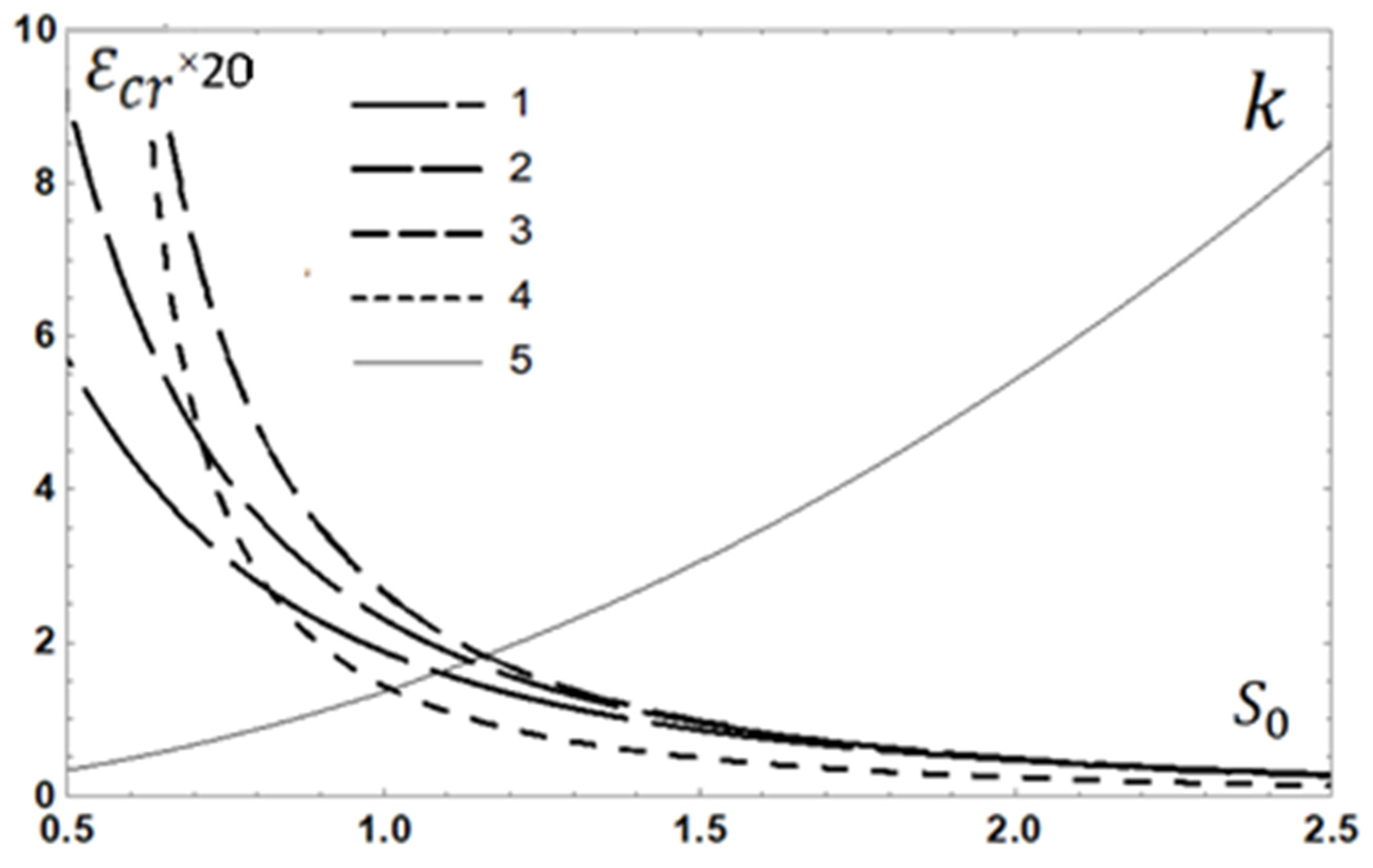
The inequality (71) represents a requirement that the wave does not break; that is, the coast is flooded without breaking the wave. This condition must always be satisfied, since our original system of equations is only valid for nonbreaking waves (note that breaking wave cannot be modeled by a well-defined function of a spatial variable). In addition, we denote by $S=\underset{x}{\max }\left|\frac{\partial \eta }{\partial x}\right|$ the steepness of the wave profile and by $S_0=\underset{y}{\max }\left|f^{\prime }\left(y\right)\right|$ the steepness of the initial wave. If we assume that the initial wave is defined by Equation (66), then $y_0$ is the fixed point of wave origination, and $k$ is the slope of the initial wave profile, such that $k=\frac{S_0^2\exp \left(1\right)}{2}.$ Figure 3 presents the dependence of the critical parameter, ${\epsilon }_{cr}$, on the slope of the initial wave for different parameter values and configurations of the ocean bottom. Here, as always, $\alpha$ represents the steepness of the sloped beach segment of the sea bottom. Curve 1 corresponds to the constant-sloped plane beach and assumes that the initial wave profile is centered at the point $y_0=1$. Curve 2 corresponds to the case where a sloped beach near the shoreline (for $x\le 1$) is continuously joined to a constant-depth ocean bottom (when $x>1$), and the initial wave is centered at the point $y_0=1.5$. Curve 3 is calculated for the same profile as Curve 2, but with the initial wave centered at the point $y_0=3$. Curve 4 corresponds to the case when the ocean bottom has a bulge (corresponding to real-world cases when a sloped beach experiences a sudden drop-off) and $y_0=3$. Curve 5 represents the dependence of the parameter $k$ on the steepness of the initial wave profile. One interesting observation drawn from Figure 3 is that, as the initial wave is centered further from shore, we see greater critical values of the parameter $\epsilon$. At the first glance, this appears to be in contradiction to the general nonlinear theory of wave propagation. According to the theory, the top of the wave moves faster than its lower part, and thus there will always exist a time, $t^{*}$, and distance, $L^{*}$, from the location of the initial wave at which the steepness of the wave $S\to \infty$, meaning that the wave collapses. Hence, as the distance which the initial wave must travel to reach the coast increases, the chance of the wave collapsing similarly increases, and this would seem to contradict the above conclusion regarding the critical values of $\epsilon$. However, there is no actual contradiction here, since the situations which we are considering assume that $\epsilon \ll 1$, and thus the nonlinearity is small and will have no effect at the distances we are considering. Furthermore, since at the beginning of the process the initial wave splits into two waves that move in opposite directions, the wave which reaches the shoreline will have a lower amplitude than the original. This causes a reduction in wave steepness which corresponds to the higher critical values, ${\epsilon }_{cr}$. Thus, while our results regarding ${\epsilon }_{cr}$ might be somewhat unexpected, they do not directly contradict the existing nonlinear theory.

Another interesting note is that the non-smooth beach profile (Curve 4 in Figure 3) sharply reduces the critical value of the parameter ${\epsilon }_{cr}$. If the smaller values of the parameter $\alpha$ correspond to smaller slopes of the beach (small ${\alpha }^{\prime }$), then, quite naturally in this case, the wave propagates at a greater distance inland where the nonlinear effects are more pronounced, implying, in turn, that the critical value, ${\epsilon }_{cr}$, should be reduced.

Recall now that the parameter $\alpha$ can be expressed as $\alpha ={\alpha }^{\prime }l/h_0$. So, if we fix ${\alpha }^{\prime }$ and change the assumed standard ocean depth, $h_0$, even if the nondimensional constant depth of the horizontal ocean bottom (which, unlike $\alpha$, is not defined in terms of $h_0$) remains 1, the partial dependence of $\alpha$ on $h_0$ will cause $\alpha$ to change, potentially creating a precipice or cavity. In particular, if an increase in the depth, $h_0$, causes a corresponding reduction of $\alpha$, then condition (71), which defines the magnitude of the parameter $\epsilon$ at which the wave collapse does not occur, should be rewritten as $\epsilon <{\epsilon }_{cr}\left(\alpha \right)/\alpha$. This is because $\epsilon$ is changed $\alpha$ times in comparison to the case when $\alpha =1$, (which follows from the fact that $\alpha =h_1/h_0$, where $h_1=h_0-\mathsf{\Delta }$ and $\mathsf{\Delta }$ is the height of the step at the point where the horizontal bottom of the ocean switches to the sloped beach). However, computations show that the values of ${\epsilon }_{cr}\left(\alpha \right)/\alpha$ are of the same order as the values of ${\epsilon }_{cr}$ at $\alpha =1$. Thus, the wave will not collapse even if the value of the parameter $\epsilon$ in this case is the same as for the case $\alpha =1$, in which there is no step (cavity) between horizontal ocean bottom and sloped beach.

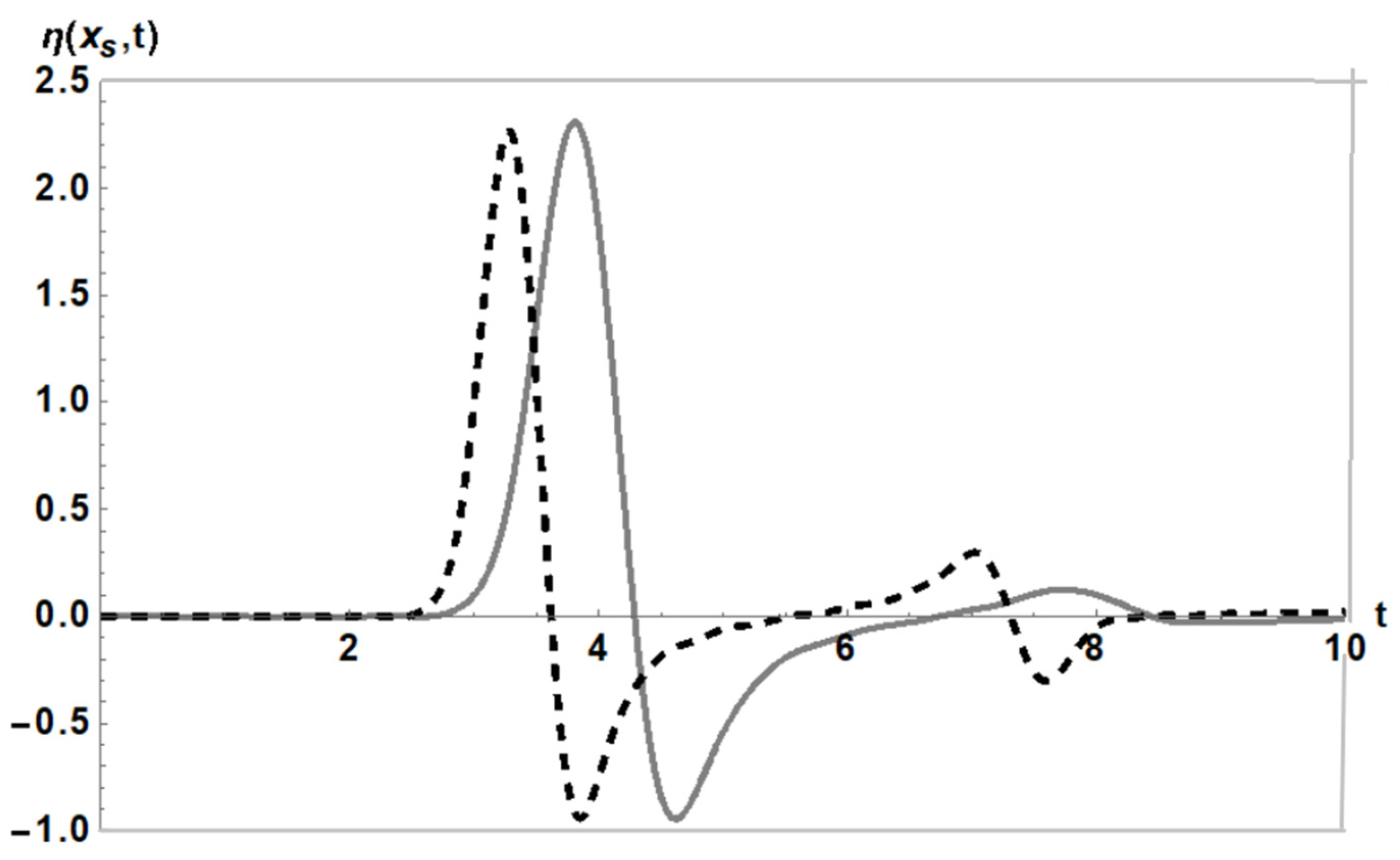
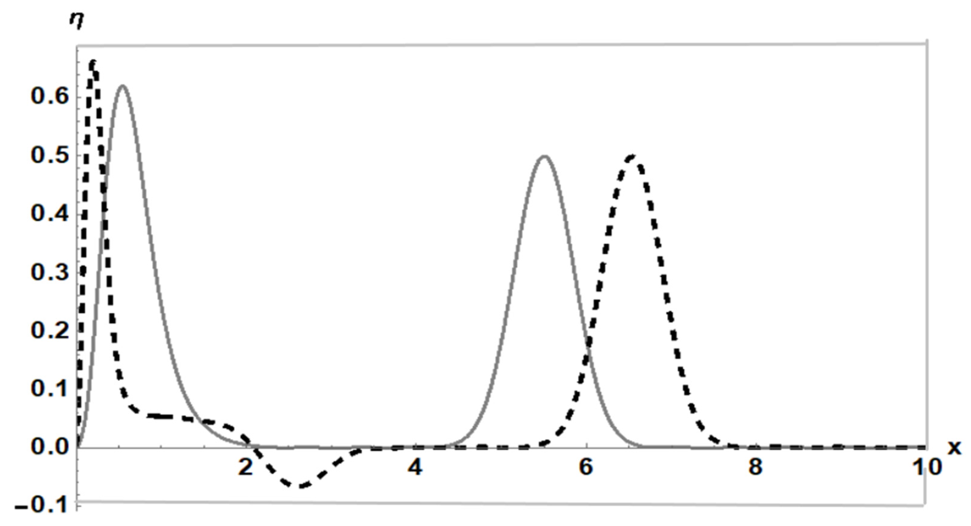
Let us consider the situation when $\alpha$ varies due to a change of the ocean depth, $h_0$, in more detail. Figure 4 illustrates the height of the wave splash on the shore as a function of time for different values of parameter $\alpha$ (and the fixed value $\epsilon =0.01$, for which there is no break of the wave). It can easily be seen that, for $\alpha =0.5$, the wave develops at the coastline much faster than for $\alpha =1$. This occurs because we are assuming that the change in $\alpha$ is due to a rescaling of the standard ocean depth, $h_0$, and greater depth causes higher wave velocity, a fact which Figure 4 reflects. Moreover, for $\alpha =0.5$ (Curve 2), we observe a second run-up and draw-back on the beach which have similar amplitudes to each other. These second splashes can be attributed to a reflection of the wave off the step in the ocean bottom that can be seen quite clearly in Figure 5 (Curve 2). Figure 5 illustrates the wave field at the time, $t=2.5$, for both $\alpha =1$ (Curve 1) and $\alpha =0.5$ (Curve 2), and we can see in Curve 2 that the primary wave, which is drawing down from the shoreline, has begun to reflect off of the underwater step.

It is worth noting that, as the parameter $\alpha$ decreases, the maximal height of the first splash decreases and the minimal height increases, whereas for the second splash, the maximal height increases and the minimal height decreases. According to the formulae (24) and (33), the horizontal run-up and draw-back of the wave is defined by the following expression:

$$x=-\epsilon x_0,\mathrm{or}x=-\frac{\epsilon }{\alpha } {\eta }_0\left(0,t\right),$$

(72)

where $x_0\left(t\right)$ is obtained by calculations based on Equation (65). If $\alpha =1$, then (72) implies that the location of the moving boundary varies according to the rule $x=-\epsilon {\eta }_0\left(0,t\right)$, but if $\alpha =0.5$, and the change of $\alpha$ took place due to the change in $h_0$, then the moving boundary varies by the same law, but the parameter $\epsilon$ in the above expression should be replaced by the product $\epsilon \alpha$. As a result, the maximal values of the run-up and draw-back for the cases $\alpha =1$ and $\alpha =0.5$ do not differ substantially, because the maximum and minimum of the function ${\eta }_0\left(0,t\right)$, which is plotted in Figure 4, do not change substantially between the two cases.

A different picture can be observed if a variation of $\alpha$ occurs due to a change in the original slope of the beach, ${\alpha }^{\prime }$. For this case, $h_0$ is fixed and $\epsilon$ remains the same for both $\alpha =1$ and $\alpha =0.5$. Therefore, if $\alpha \ne 1$, from (72), we see that $x=-\frac{\epsilon }{\alpha }{\eta }_0\left(0,t\right)$. This implies that, for $\alpha =0.5$, the horizontal run-up and draw-back on the shore are becoming practically two times greater. In this case, the characteristic time, $t_0$, also does not change, and therefore no time lag takes place.

5. Summary/Conclusions

In this paper, we proposed a quasi-linear theory of tsunami run-up and run-down on a beach with complex seafloor geometry, which can be modeled by a piecewise linear function. Our goal was to develop an approximate analytic solution which, while primarily theoretical in nature, is thus applicable to cases where purely analytic results have not been found. Due to the nature and size of tsunami phenomena, they can be modeled by using the shallow-water wave equations, and we chose the nonlinear versions of these equations for full accuracy. Once the nonlinear shallow-water wave equations were nondimensionalized, we obtained the desired degree of approximation by reducing our system to a quasi-linear system, using the method of perturbations, and considering only terms of leading order in the small parameter $\epsilon$.

We conclude that the obtained solution is valid only if $\epsilon$ is assumed to be small enough that the wave does not break. We then calculate the critical value, ${\epsilon }_{cr}$, of the parameter $\epsilon$ such that the wave does not break for all $\epsilon <{\epsilon }_{cr}$.

While the equations which result are linear, a degree of nonlinearity is nonetheless present due to the behavior of the moving boundary, which is implicit in our modified spatial variable. Application of the integral transformation led to two distinct problems: a boundary-value problem for the transformed variable and a Sturm–Liouville problem for the arbitrary kernel of the transformation. The problem for the transformed variable has a simple solution, and while finding a particular solution for the kernel requires a particular choice of the seafloor function, we are able to use the properties of a Sturm–Liouville problem to obtain an inversion formula and can thus present general formulae which fully describe the tsunami run-up and draw-down for any beach configuration.

Having found our solution which is valid for any piecewise continuous seafloor profile, we then apply it to the case of a constant-sloped beach which leads (not necessarily continuously) to a horizontal constant-depth sea bottom—a case for which previously only numerical results had been found. For this case, we obtain formulae for both the kernel function and its eigenvalues. We are able once again to calculate the critical value of $\epsilon$ and plot our results for various permissible values of the parameters. These results initially appear to contradict existing nonlinear theory, but a closer analysis reveals no contradictions. We investigated a case where the slope of the first beach segment changes due to an adjustment in the characteristic ocean depth (and thus changes relative to the horizontal sea bottom) and determined that even in this case no additional restrictions are needed on the parameters.

Ultimately, we were successful in each of our goals. We were able to find a set of general formulae which describe an analytic solution within order $O\left(\epsilon \right)$ for an arbitrary beach configuration. The full power of the simplicity of our approach was seen clearly when we computed results for the case of the two-part (constant-sloped leading to constant-depth) beach, which proved to be too complex for analytic research.

References

- Stoker, J.J. Water Waves: The Mathematical Theory with Applications; Wiley-Interscience: Hoboken, NJ, USA, 1957. [Google Scholar]
- Volsinger, N.E.; Klevanny, K.A.; Pelinovsky, E.N. Long-Wave Dynamics of Coastal Zone; Gidrometeoizdat: Leningrad, Russia, 1989. [Google Scholar]
- Carrier, G.F.; Greenspan, H.P. Water waves of finite amplitude on a sloping beach. J. Fluid Mech. 1958, 4, 97–109. [Google Scholar] [CrossRef]
- Carrier, G.F.; Wu, T.T.; Yeh, H. Tsunami runup and drawdown on a sloping beach. J. Fluid Mech. 2003, 475, 79–99. [Google Scholar] [CrossRef]
- Kânoglu, U. Nonlinear evolution and runup-rundown of long waves over a sloping beach. J. Fluid Mech. 2004, 513, 363–372. [Google Scholar] [CrossRef]
- Kânoglu, U.; Synolakis, C. Initial value problem solution of nonlinear shallow water-wave equations. Phys. Rev. Lett. 2006, 97, 148501–148504. [Google Scholar] [CrossRef] [PubMed]
- Liu, P.L.-F.; Lynett, P.; Synolakis, C.E. Analytical solutions for forced long waves on a sloping beach. J. Fluid Mech. 2003, 478, 101–109. [Google Scholar] [CrossRef] [Green Version]
- Didenkulova, I.; Pelinovsky, E. Nonlinear wave effects at the non-reflecting beach. Nonlin. Process. Geophys. 2012, 19, 1–8. [Google Scholar] [CrossRef] [Green Version]
- Rybkin, A.; Pelinovsky, E.; Didenkulova, I. Nonlinear wave run up in bays of arbitrary cross-section: Generalization of the Carrier-Greenspan approach. J. Fluid Mech. 2014, 748, 416–432. [Google Scholar] [CrossRef]
- Rybkin, A.; Nicolsky, D.; Pelinovsky, E.; Buckel, M. The Generalized Carrier–Greenspan Transform for the Shallow Water System with Arbitrary Initial and Boundary Conditions. Water Waves 2020, 3, 267–296. [Google Scholar] [CrossRef]
- Chugunov, V.; Fomin, S.; Noland, W.; Sagdiev, B. Tsunami runup on a sloping beach. Comput. Math. Methods 2020, 2, e1081. [Google Scholar] [CrossRef] [Green Version]
- Pelinovskij, E.N. Tsunami Wave Hydrodynamics; IAP Russian Academy of Science: Nizhny Novgorod, Russia, 1996. [Google Scholar]
- Chugunov, V.; Fomin, S.; Shankar, R. Influence of underwater barriers on the distribution of tsunami waves. J. Geophys. Res. Ocean. 2014, 119, 7568–7591. [Google Scholar] [CrossRef]
- Koshlyakov, N.S.; Gliner, E.B.; Smirnov, M.M. Partial Differential Equations of Mathematical Physics; Visshaya Shkola: Moscow, Russia, 1970. [Google Scholar]
Figure 2.
A schematic of the runup phenomenon used in the current paper.
Figure 3.
Dependence of the critical value, , and parameter from the steepness of the initial wave, , for the different initial wave locations, , and different geometries of the seafloor given by the parameter : , and (linear beach, no step); , and (linear beach, no step); , and (linear beach, no step); , and (sloping beach with vertical step down (cavity) connected with horizontal seafloor); and .
Figure 4.
Dynamics of the height of the water splash above the still water level at the moving boundary for the smooth case (, solid line) and for the case when the sloping beach has a vertical step down to the flat horizontal seafloor (, dashed).
Figure 5.
The shape of the wave at
for the smooth beach is (solid line), and for the beach with the vertical step, (dashed line).
Publisher’s Note: MDPI stays neutral with regard to jurisdictional claims in published maps and institutional affiliations. |
© 2022 by the authors. Licensee MDPI, Basel, Switzerland. This article is an open access article distributed under the terms and conditions of the Creative Commons Attribution (CC BY) license (https://creativecommons.org/licenses/by/4.0/).
Share and Cite
MDPI and ACS Style
Chugunov, V.; Fomin, S.; Sagdiev, B. Quasi-Linear Model of Tsunami Run-Up on a Beach with a Seafloor Described by the Piecewise Continuous Function. Geosciences 2022, 12, 445. https://0-doi-org.brum.beds.ac.uk/10.3390/geosciences12120445
AMA Style
Chugunov V, Fomin S, Sagdiev B. Quasi-Linear Model of Tsunami Run-Up on a Beach with a Seafloor Described by the Piecewise Continuous Function. Geosciences. 2022; 12(12):445. https://0-doi-org.brum.beds.ac.uk/10.3390/geosciences12120445
Chicago/Turabian StyleChugunov, Vladimir, Sergei Fomin, and Bayazit Sagdiev. 2022. "Quasi-Linear Model of Tsunami Run-Up on a Beach with a Seafloor Described by the Piecewise Continuous Function" Geosciences 12, no. 12: 445. https://0-doi-org.brum.beds.ac.uk/10.3390/geosciences12120445
Note that from the first issue of 2016, this journal uses article numbers instead of page numbers. See further details here.