Extending the Range of Milankovic Cycles and Resulting Global Temperature Variations to Shorter Periods (1–100 Year Range)

Abstract

The Earth’s revolution is modified by changes in inclination of its rotation axis. Its trajectory is not closed and the equinoxes drift. Changes in polar motion and revolution are coupled through the Liouville–Euler equations. Milanković (1920) argued that the shortest precession period of solstices is 20,700 years: the summer solstice in one hemisphere takes place alternately every 11,000 year at perihelion and at aphelion. Milanković assumed that the planetary distances to the Sun and the solar ephemerids are constant. There are now observations that allow one to drop these assumptions. We have submitted the time series for the Earth’s pole of rotation, global mean surface temperature and ephemeris to iterative Singular Spectrum Analysis. iSSA extracts from each a trend a 1 year and a 60 year component. Both the apparent drift of solstices of Earth around the Sun and the global mean temperature exhibit a strong 60 year oscillation. We monitor the precession of the Earth’s elliptical orbit using the positions of the solstices as a function of Sun–Earth distance. The “fixed dates” of solstices actually drift. Comparing the time evolution of the winter and summer solstices positions of the rotation pole and the first iSSA component (trend) of the temperature allows one to recognize some common features. A basic equation from Milankovic links the derivative of heat received at a given location on Earth to solar insolation, known functions of the location coordinates, solar declination and hour angle, with an inverse square dependence on the Sun–Earth distance. We have translated the drift of solstices as a function of distance to the Sun into the geometrical insolation theory of Milanković. Shifting the inverse square of the 60 year iSSA drift of solstices by 15 years with respect to the first derivative of the 60 year iSSA trend of temperature, that is exactly a quadrature in time, puts the two curves in quasi-exact superimposition. The probability of a chance coincidence appears very low. Correlation does not imply causality when there is no accompanying model. Here, Milankovic’s equation can be considered as a model that is widely accepted. This paper identifies a case of agreement between observations and a mathematical formulation, a case in which an element of global surface temperature could be caused by changes in the Earth’s rotation axis. It extends the range of Milankovic cycles and resulting global temperature variations to shorter periods (1–100 year range), with a major role for the 60-year oscillation).

1. Introduction

For over a century and a half, geological evidence has been put forward to argue that Earth had undergone cyclical changes in climate [1]. Adhémar [2] described the long periodicities associated with glacial and interglacial cycles that were explained sixty years later by the mathematical theory of climate due to Milankovic [3]. A geometrical derivation shows that the insolation W received at a location with coordinates $\phi$ (latitude) and $\psi$ (longitude) is given by the (fundamental, yet simple) equation (Equation (20), p. 15, [3]):

$${\displaystyle \frac{dW}{dt}}={\displaystyle \frac{I_0}{{\rho }^2}}[sin\phi sin\delta +cos\phi cos\delta cos(\omega +\psi )]$$

(1)

where $\rho$ is the Sun-Earth distance, $\delta$ the Sun’s declination and $\omega$ its hour angle. It is generally considered that the shortest Milanković cycle is the 19,000 year precession cycle (e.g., [4,5]). The Earth’s eccentricity being quite small ($e=$ 0.016), it is legitimate at first to consider that, over such long durations, $\rho$ and $\delta$ are constant. Thus, Ref. [3] assumes that all climate variations arise because of movements of the rotation axis (i.e., of the pole).

These climate variations are recorded for instance by benthic marine sediments. Thus, Lopes et al. [5] were able to extract from the ${\delta }^{18}O$ series of Lisiecki and Raymo [6] all the Milanković components calculated with the Laskar et al. [4] model, that is all variations in insolation, eccentricity, precession and obliquity of the Earth’s rotation axis.

To first order, the rotation axis is perturbed by the conjugate effects of the Moon and Sun (e.g., [7,8]), resulting for instance in the luni-solar tides (e.g., [9,10,11,12]). Over longer periods, the Jovian planets are the main source of perturbations of the rotation axis (cf. [4,13]), giving rise to variations in precession, obliquity and eccentricity.

It has recently been shown, based on observations, that the Jovian planets exert perturbations both on Earth and in the Sun at much shorter periods (centuries to years and less) (e.g., [14,15,16,17,18,19]). These perturbations affect solar activity, therefore sunspots [15], as well as the rotation axis [16], and therefore Earth’s climate. This could explain the links between geomagnetism and climate (e.g., [20,21]).

Another source of perturbation of the Earth’s rotation axis is the precession of equinoxes, associated with Kepler’s second law (conservation of areas). There are four sources of precession of Earth’s equinoxes, that is rotation of the whole orbit (revolution).

(1)

The first is associated with Kepler’s laws. In the case of a central field and an elliptical orbit, for the orbit to be closed, it is necessary and sufficient that the orbit’s angular change after n revolutions be of the form $\Delta \phi =2\pi m/n$, where m is the number of full revolutions necessary for the planet to recover its initial position. There are only two central fields in which $\Delta \phi$ is a rational fraction of $2\pi$, ensuring closed orbits, that is fields in $r^2$ and $1/r$, the latter being the case of our solar system (cf. [22]).

(2)

The second involves the joint effects of the Moon and Sun. Let us quote d’Alembert ([23], p. 14): “Enfin, l’inclinaison de l’axe terrestre au plan de l’ecliptique doit modifier aussi l’action du Soleil; car selon que cet axe sera différemment incliné, il fera à chaque point de l’ecliptique un angle différent avec la ligne qui joint les centres de la Terre et du Soleil; par conséquent la quantité et la loi de l’action du Soleil, dépend de l’inclinaison de l’axe, et c’est aussi ce que l’analyse apprend.”

As clearly stated by [7] and later [8], the planet’s revolution is modified by changes in inclination of the rotation axis, principally due to the joint actions of the Moon (for 2/3rds) and Sun (for 1/3rd). One is no longer in case 1: despite the fact that the field is a central one, the trajectory is not closed anymore. d’Alembert ([23], p. 52) estimates the drift of the equinoxes to be about 50” per year, that is a precession period of 25,920 year.

The two other processes are relativistic.

(3)

The Sun containing 99% of the total mass of the solar system, [24] shows that the planet’s revolution about the Sun produces an additional precession of about 3.8” per century, or a period of some 33 million years.

(4)

Because the Sun is actually a huge rotating mass, there is an additional relativistic component of precession, with a period on the order of 5.8 million years [25].

For Newton, planetary bodies attract (or repel) the oceans (and atmospheres) and this re-organization of masses modifies the rotation axis. For d’Alembert, Lagrange, Laplace and Poincaré, changes in polar motion and revolution are coupled and involve the luni-solar torques, as in a top. Re-organization of Earth’s fluid envelopes (e.g., tides) follows.

As [3] writes, precession of the equinoxes is actually due to the joint attraction of the Moon and Sun on the Earth’s equatorial bulge and its period is in theory 26,000 year. Because the Earth itself rotates, areolar velocities vary between perihelion and aphelion (Kepler’s second law); because of centrifugal forces, a precession with a period of 19,000 year appears. So the precession of equinoxes undergoes a double periodicity, with a mean of 22,500 year (half period 11,250 year). Indeed, Milanković ([3], p. 221) writes that the first precession of perihelion (for us solstices) is 20,700 Julian years and that the consequence of this precession is that the Summer solstice in one hemisphere (when that hemisphere receives maximum insolation) takes place alternately every 11,000 year at perihelion (thus a warmer Summer) and aphelion (thus a cooler Summer). The difference in insolation (energy received by Earth) between maximum and minimum is a function of eccentricity.

The 26,000 year period of precession has first been determined in the frame of Newtonian physics by d’Alembert ([23]). It is rather close to the first precession cycle of 19,000 year in Milanković ([3]) theory. When Milanković makes the assumption that the planetary distances to the Sun and the solar ephemerids are constant, he can estimate climate maxima, but not their smooth transitions between equinoxes and solstices. Today, we have access to observations that allow one to drop the hypotheses that $\rho$, $\delta$ and $\omega$ in Equation (1) are constant. Thus, we can evaluate the consequences of changes in the position of the rotation axis on, for instance, atmospheric temperature, that is the main parameter in Milanković’s theory of climate.

2. The Data: Temperature, Pole Motion, and Solar Ephemerids

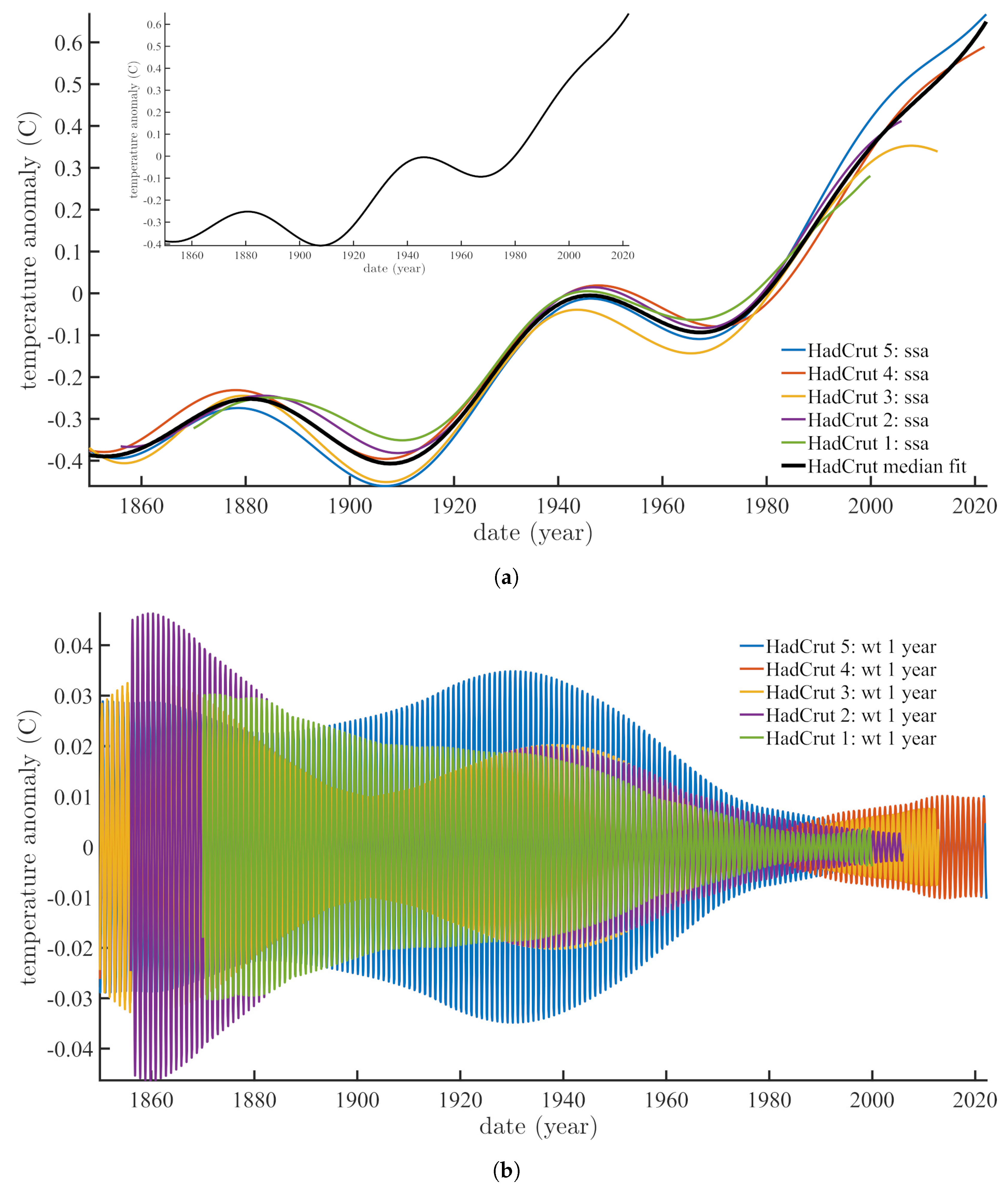
2.1. Mean Global Temperatures

We have used the data series maintained by the Hadley Center for Climate Prediction and Research under the name HadCrut. In order to have an idea of the reliability of the data, we have selected five successive sets of HadCrut data: HadCrutv from 1870 to 2000 ([26], https://crudata.uea.ac.uk/cru/data/crutem1, accessed on 2 June 2022); HadCrut2 from 1856 to 2006 ([27], https://crudata.uea.ac.uk/cru/data/crutem2, accessed on 2 June 2022); HadCrut3 from 1850 to 2014 ([28], https://crudata.uea.ac.uk/cru/data/crutem3, accessed on 2 June 2022); HadCrut4 from 1850 to 2021 ([29], https://crudata.uea.ac.uk/cru/data/crutem4/, accessed on 2 June 2022) and HadCrut5 from 1850 to 2022 ([30], https://crudata.uea.ac.uk/cru/data/temperature/, accessed on 2 June 2022). Figure 1a shows all the data, and Figure 1b their Fourier transforms. There are rather significant differences between the data series, for instance between 1940 and 2020 in HadCrut3 (yellow curve) vs. HadCrut5 (blue curve). Differences become larger after 1950, to the point that HadCrut3 has a plateau after 2000 when HadCrut5 grows linearly since 1960. We have already worked on these data sets [31] and pointed out these differences [32], Figure 4. These differences of course result in differences in the Fourier spectra of Figure 1. As a result, the dominant spectral peak shifts from 60 to 80 year, a topic discussed in several papers [32,33,34,35].

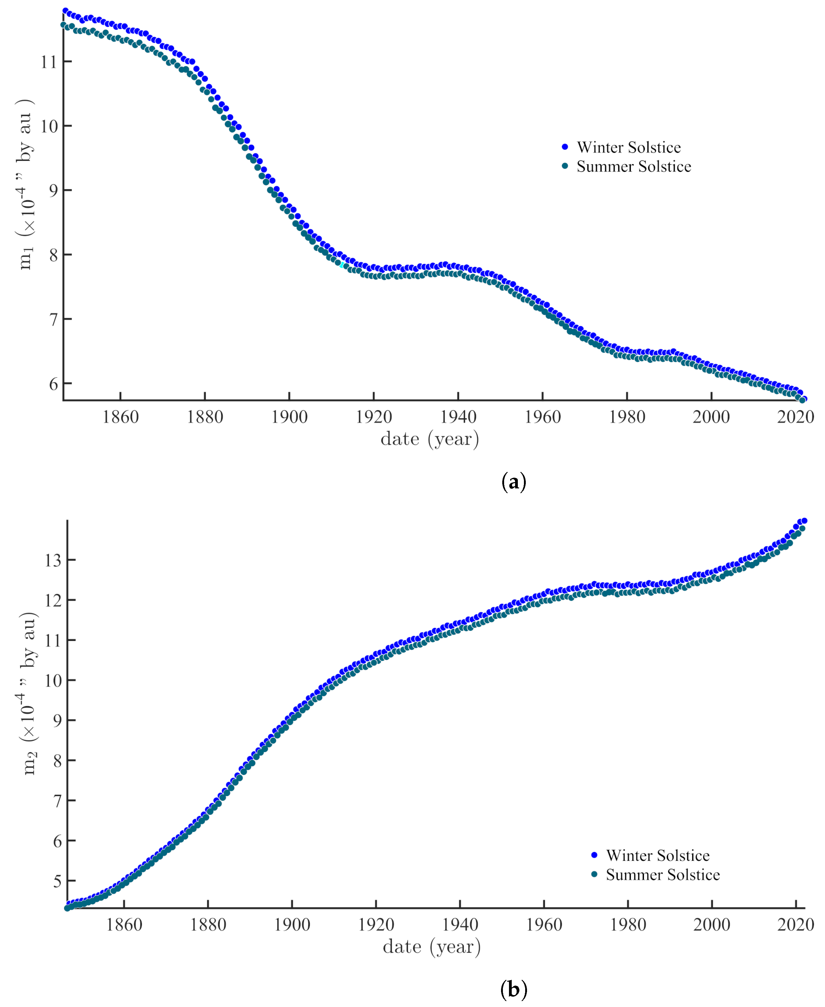
2.2. Solar Ephemerids

We have obtained the Sun’s ephemerids from 1846 to the present from Institut de Mécanique Céleste et du Calcul des Ephémérides (IMCCE, http://vo.imcce.fr/webservices/miriade/?forms, accessed on 2 June 2022). We do not present a figure with the raw data: the Earth orbit’s eccentricity is so small that an annual oscillation since 1846 would transform into an unreadable quasi-sinus with 176 oscillations on the 15 cm (or so) width of the figure, that is 14 oscillations per cm.

2.3. Rotation Pole and Length of Day

The motions of the rotation pole and variations in rotation velocity are available at the International Earth Rotation Reference Systems Service (IERS, https://www.iers.org/IERS/EN/DataProducts/EarthOrientationData/eop.html, accessed on 2 June 2022). They consist in the couple of coordinates ($m_1$, $m_2$) of motion of the rotation pole PM (see [16,36]) and the length of day lod (e.g., [12]). We have selected data set EOP C01 IAU19801. Figure 2a,b respectively show the evolution of the couple ($m_1$, $m_2$) since 1946 and of lod since 1962. We have used the semi-annual lod data provided by Stephenson and Morrison ([37]) for the period 1832–1997, combined with the IERS data, resulting in the mean curve between 1832 and 2022 shown in Figure 2c (cf. [38]).

3. Extraction and Analysis of the Trends and Annual Oscillations

3.1. Methods: SSA

As in a number of previous papers, e.g., [16,39,40], we have submitted time series to iterative Singular Spectrum Analysis (iSSA) and we will now do the same for the rotation, temperature and ephemeris time series presented in the previous section. We refer the reader to these papers and to the Golyandina and Zhigljavsky’s book ([41]) for the SSA method, to [42] for properties of the Hankel and Toeplitz matrices that it uses, and to [43] for the singular value decomposition algorithm SVD).

Following a suggestion by an anonymous reviewer, we now propose a short but more detailed summary of the method.

Let us consider a discrete (non-zero) time series (${\mathcal{X}}_N$) of length N (N>2): ${\mathcal{X}}_N=(x_1,\dots ,x_N).$

• Step 1: embedding step

${\mathcal{X}}_N$ is divided into K segments of length segments of length L in order to build a matrix $\mathbf{X}$ with dimension $K\times N$ where $K=N-L+1$ will condition our decomposition. This is the first “tuning knob”. Integrating $\mathbf{X}$ yields a Hankel matrix:

$$\mathbf{X}=\left(\begin{array}{cccc}{x}_1& x_2& x_3\cdots & x_K\\ x_2& x_3& x_4\cdots & x_{K+1}\\ x_3& x_4& x_5\cdots & x_{K+2}\\ ⋮& ⋮& ⋮\ddots & ⋮\\ x_L& x_{L+1}& x_{L+2}\cdots & x_N\end{array}\right)$$

(2)

Embedding, the first step in a SSA, consists in projecting the one-dimensional time series in a multidimensional space of series ${\mathcal{X}}_N$ such that vectors $X_i={(x_i,\dots ,x_{i+L-1})}^t$ belong to ${\mathcal{R}}^L$ where $K=N-L+1$. The parameter that controls the embedding is L, the size of the analyzing window, an integer between 2 and $N-1$. The Hankel matrix has a number of symmetry properties: its transpose ${\mathbf{X}}^t$, called the trajectory matrix, has dimension K. Embedding is a compulsory step in the analysis of non-linear series. It consists formally in the empirical evaluation of all pairs of distances between two offset vectors, delayed (lagged) in order to calculate the correlation dimension of the series.

• Step 2: Decomposition in singular values—SVD

SVD of non-zero trajectory matrix X (dimensions $L\times K$) takes the shape:

$$\mathbf{X}=\sum _{i=1}^d\sqrt{{\lambda }_i}{U}_i{V}_i^t$$

(3)

where the eigenvalues ${\lambda }_i$ ($i=1,\dots ,L$) of matrix $\mathbf{S}={\mathbf{XX}}^T$ are arranged in order of decreasing amplitudes. Eigenvectors $U_i$ and $V_i$ are given by:

$$V_i={\mathbf{X}}^T{U}_i/\sqrt{{\lambda }_i}$$

(4)

The $V_i$ form an orthonormal basis and are arranged in the same order as the ${\lambda }_i$. Let ${\mathbf{X}}_i$ be a part of matrix $\mathbf{X}$ such that:

$${\mathbf{X}}_i=\sqrt{{\lambda }_i}{U}_i{V}_i^t.$$

(5)

Embedding matrix X can then be represented as a simple linear sum of elementary matrices X${}_i$. If all eigenvalues are equal to 1, then decomposition of X into a sum of unitary matrices is:

$$\mathbf{X}={\mathbf{X}}_1+{\mathbf{X}}_2+\dots +{\mathbf{X}}_d$$

(6)

d being the rank of X ($d=\mathrm{rank}\mathbf{X}=max\left\{i\right|{\lambda }_i>0\}$) SVD allows one to write X as a sum of d unitary matrices, defined in a univocal way.

Let us now discuss the nature and the characteristics of the embedding matrix. Its rows and columns are sub-series of the original time series (or signal). The eigenvectors $U_i$ and $V_i$ have a time structure, and they can be considered as a representation of temporal data. Let X be a suite of L lagged parts of (X and $X_1,\dots ,X_K$) the linear basis of its eigenvectors. If we let:

$$Z_i=\sum _{i=1}^d\sqrt{{\lambda }_i}{V}_i$$

(7)

with $i=1,\dots ,d$, then the relation (5) can be written:

$$\mathbf{X}=\sum _{i=1}^d{U}_i{Z}_i^t$$

(8)

that is for the jth elementary matrix:

$$X_j=\sum _{i=1}^d{z}_{ji}{U}_i$$

(9)

where $z_{ji}$ is a component of vector Z${}_i$. This means that vector Z${}_i$ is composed of the ith components of vector X${}_j$. In the same way, if we let:

$$Y_i=\sum _{i=1}^d\sqrt{{\lambda }_i}{U}_i$$

(10)

we obtain for the transposed trajectory matrix:

$$X_j^t=\sum _{i=1}^d{U}_i{Y}_i^t$$

(11)

that corresponds to a representation of the lagged vectors in the orthogonal basis ($V_1$,…,$V_d$). One sees why SVD is a very good choice for the analysis of the embedding matrix, since it provides two different geometrical descriptions.

• Step 3: reconstruction

As we have seen, ${\mathbf{X}}_i$ matrices are unit matrices, and one can “re-group” these matrices into a physically homogeneous quantity. This is the second “tuning knob” of SSA. In order to regroup the unit matrices, one divides the set of indices {i${}_1$,…,i${}_d$} into m disjoint subsets of indices $\{I_1,\dots ,I_m\}$.

Let I be the grouping of p indices of $I=\{i_1,i_2,\dots ,i_p\}$; because (6) is linear, then the resulting matrix X${}_I$ that regroups indices I can be written:

$${\mathbf{X}}_I={\mathbf{X}}_{I1}+{\mathbf{X}}_{I2}+\dots +{\mathbf{X}}_{Im}$$

(12)

This step is called regrouping the eigen-triplets ($\lambda$, U and V). In the limit case $m=d$, (12) becomes exactly (6), and we again find the unit matrices.

Next, how can one associate pairs of eigen-triplets? This means separating the additive components of a time series. One must first consider the concept of separability.

Let $\chi$ be the sum of two time series ${\chi }^{\left(1\right)}$ and ${\chi }^{\left(2\right)}$ such that $x_i=x_i^{\left(1\right)}+x_i^{\left(2\right)}$ for any $i\in [1,N]$. Let L be the analyzing window (with fixed length), X, X${}^{\left(1\right)}$ and X${}^{\left(2\right)}$ be the embedding matrices of series $\chi$, ${\chi }^{\left(1\right)}$ and ${\chi }^{\left(2\right)}$. These two sub-series are separable (even weakly) in Equation (6) if there is a collection of indices $\mathcal{I}\subset \{1,\dots ,d\}$ such that ${\mathbf{X}}^{\left(1\right)}={\sum }_{i\in \mathcal{I}}{\mathbf{X}}_i$, respectively, if there is a collection of indices such that ${\mathbf{X}}^{\left(1\right)}={\sum }_{i\notin \mathcal{I}}{\mathbf{X}}_i$.

In the case when separability does exist, the contribution of ${\mathbf{X}}^{\left(1\right)}$ for instance corresponds to the ratio of associated eigenvalues (${\sum }_{i\in \mathcal{I}}{\lambda }_i$) to total eigenvalues (${\sum }_{i=1}^d{\lambda }_i$).

So, regrouping SVD components can be summarized by the decomposition into several elementary matrices, whose structure must be as close as possible to a Hankel matrix of the initial trajectory matrix (this is true on paper only, in reality things are much more difficult).

• Step 4: the diagonal mean, also known as the hankelization step

The next, final step consists in going back to data space, that is to calculate time series with length N associated with sub-matrices ${\mathbf{X}}_I$. Let Y be a matrix with dimension $L\ast K$ and for each element $y_{ij}$ we have $1⩽i⩽L$ and $1⩽j⩽K$. Let $L^{*}$ be the minimum and $K^{*}$ be the maximum. One always has $N=L+K-1$. Finally, let $y_{ij}^{*}=y_{ij}\mathrm{if}L<K\mathrm{and}{y}_{ij}^{*}=y_{ji}$ otherwise. The diagonal average applied to $k^{th}$ index of time series y associated with matrix Y gives:

$$y_k=\left\{\begin{array}{ccc}\frac{1}{k}& {\displaystyle \sum _{m=1}^k}{y}_{m,k-m+1}^{*}& 1⩽k⩽L^{*}\\ \frac{1}{L^{*}}& {\displaystyle \sum _{m=1}^{L^{*}}}{y}_{m,k-m+1}^{*}& L^{*}⩽k⩽K^{*}\\ \frac{1}{N-K+1}& {\displaystyle \sum _{m=k-K*+1}^{N-K*+1}}{y}_{m,k-m+1}^{*}& K^{*}⩽k⩽N^{*}\end{array}\right.$$

(13)

The relation (13) corresponds to the mean of the element on the anti-diagonal $i+j=k+1$ of the matrix. For $k=1$, $y_1=y_{1,1}$. For $k=2$, $y_2=(y_{1,2}+y_{2,1})/2$, etc.

As mentioned above, step 3 is the most difficult part. We have chosen one approach among many others: iterative SSA (iSSA). Since the relation (6) is linear, we can iterate the decomposition. We start with a small value of L (we are looking for the longest period) that we increase until getting a quasi-Hankel matrix (step 1 and 2). We then extract the corresponding lowest frequency component that it subtracted from the original signal. We again increase the value of L to find the next component (shortest period). The algorithm stops when no pseudo-cycle can be detected or extracted. In this way, we scan the series from low to high frequencies.

Figure 3a shows the first oscillatory iSSA component of lod that has a period of 1 year.

3.2. Methods: Wavelets

In order to check the quality of iSSA, we have compared some of the iSSA results with those obtained with the method of continuous wavelets, that is widely used in the literature. Figure 3b shows the scalogram (i.e., the continuous wavelet transform) of lod since 1962 (Figure 2b). We have selected a Morlet wavelet. Between the dashed red lines are the ordinates of the wavelet coefficients associated with the 1 year oscillation. Given the property of information redundancy of the wavelet kernels, one can extract the ridge in the scales covered by the 1 year periodicity and reconstruct the signal [44]. The (wavelet) reconstructed annual component of lod is shown as the black curve in Figure 3a. The comparison is good but not perfect: the modulation of the iSSA curve (in red) is smoother than that of the wavelet reconstruction. The similarity of the two curves in Figure 3a together give us confidence that iSSA can correctly extract the annual components of the three time series introduced in Section 2.

The continuous wavelet transform ([45]) of a signal s with respect to the analyzing wavelet $\psi$, in the form of convolution product, follows the relationship,

$$\mathcal{W}[\psi ,s](t,a)\equiv [s\ast {\tilde{\psi }}_a]\left(t\right)$$

(14)

where ${\tilde{\psi }}_a\equiv a^{-1}{\psi }^{*}(-t/a)$ with a > 0 s the dilatation parameter and ${}^{*}$ the complex conjugate. We are interested here in the analysis of oscillating signals and we shall use a complex analyzing wavelets of the following form,

$${\psi }_a\left(t\right)={\displaystyle \frac{1}{a}}{A}_{\psi }({\displaystyle \frac{t}{a}})\exp [i{\phi }_{\psi }({\displaystyle \frac{t}{a}})]$$

(15)

where $A_{\psi }\left(t\right)$ is a real-valued envelope and ${\phi }_{\psi }\left(t\right)$ is the phase term. Let us define Morlet’s wavelets as follows, whose Fourier transform is given by,

$${\widehat{\psi }}_{a,M}^{\pm }\left(u\right)=\sqrt{8\pi \sigma }\exp [-8{\pi }^2{\sigma }^2{(au\mp {\displaystyle \frac{1}{2}})}^2]$$

(16)

(16) shows that a wavelet is typically a band-pass Gaussian-like filter with a central frequency $u_c={\displaystyle \frac{1}{2a}}$. We may then consider that ${\psi }_{a,M}^{+}$ have a band-pass limited to positive frequencies, while ${\psi }_{a,M}^{-}$ have a band-pass restricted to negative frequencies. $\sigma >0$ controls the duration of the Gaussian envelope (i.e., the time resolution $\tau$).

The wavelet Formula (14) can be inverted under certain conditions. Let us consider the following operator,

$$\begin{array}{c}\hfill \begin{array}{cc}\hfill \mathcal{M}[\chi ,r]\left(t\right)& ={\int }_{-\infty }^{+\infty }{\int }_0^{+\infty }r(b,a){\chi }_a(t-b){\displaystyle \frac{da}{a}}db\hfill \\ \hfill & ={\int }_0^{+\infty }[r(.,a)\ast {\chi }_a(.)]\left(t\right){\displaystyle \frac{da}{a}}\hfill \end{array}\end{array}$$

(17)

$\mathcal{M}$ maps a function r over the time-dilation half-space onto a function of time by superimposing the wavelets ${\chi }_a(.,-b)$. $\mathcal{M}$ is called the wavelet synthesis. The following relation holds for arbitrary $\psi$ and $\chi$ functions,

$$\mathcal{M}[\chi ,\mathcal{W}(\psi ,s)]={\mathcal{F}}^{-1}\left\{\left[{\widehat{m}}_{\psi ,\chi }\right]{\mathcal{F}}_s\right\}$$

(18)

and for $u\ne 0$,

$${\widehat{m}}_{\psi ,\chi }\left(u\right)={\int }_0^{+\infty }{\widehat{\psi }}^{*}\left(au\right)\widehat{\chi }\left(au\right){\displaystyle \frac{da}{a}}$$

(19)

relations (18) and (19), in which $\mathcal{F}$ is the Fourier transform, ${}^{*}$ the complex conjugate and ${\widehat{m}}_{\psi ,\chi }$ acts as a multiplication operator. Note that because the oscillation of $\psi$, we have $\widehat{\psi }\left(0\right)=0$ and the integral is convergent. In particular, we may choose $\chi$ in such a way that,

$${\widehat{m}}_{\psi ,\chi }\left(u\right)=1$$

(20)

A sufficient condition for such reconstruction $\chi$ to exist is,

$$0<C_{\psi }={\int }_0^{+\infty }{\left|\widehat{\psi }(\pm a)\right|}^2{\displaystyle \frac{da}{a}}<\infty$$

(21)

in which case, $\psi$ is called admissible. For an admissible $\psi$, a possible choice would be,

$$\chi \left(t\right)={\displaystyle \frac{1}{C_{\psi }}}\psi \left(t\right)$$

(22)

and the reconstruction formula (cf. [45]) becomes,

$$s\left(t\right)={\displaystyle \frac{1}{C_{\psi }}}{\int }_0^{+\infty }[\mathcal{W}(\psi ,s)(.,a)\ast {\chi }_a(.)]\left(t\right){\displaystyle \frac{da}{a}}$$

(23)

One last concept needs to be clarified here: the notion of ridge function of oscillating signals. There are two concepts of frequency associated with wavelet transform (14). The first one is the instantaneous phase velocity of the wavelets coefficients,

$${\displaystyle \frac{d{\mathsf{\Phi }}_{t,a}}{dt}}={\displaystyle \frac{d}{dt}}\arg \mathcal{W}[\psi ,s](t,a)$$

(24)

and the second concept associates the scale a with the frequency ${\displaystyle \frac{u_0}{a}}$, where $u_0$ is the central frequency of the undilated wavelet. The ridge is defined to be the set of points where both concepts coincide,

$${\displaystyle \frac{d{\mathsf{\Phi }}_{t,a}}{dt}}={\displaystyle \frac{\pi }{a_s\left(t\right)}}$$

(25)

To give an example, for a monochromatic signal of the form $s\left(t\right)=A_s\exp \left[2i\pi u_{0}t\right]$, the Morlet’s wavelet transform is,

$$\mathcal{W}[{\psi }_M^{\pm },s]={\displaystyle \frac{\sqrt{8\pi \sigma A_s}}{a}}\exp [i{\mathsf{\Phi }}_{t,a}(t)]\exp [-8{\pi }^2{\sigma }^2{(a{u}_s\mp {\displaystyle \frac{1}{2}})}^2]$$

(26)

where ${\mathsf{\Phi }}_{t,a}=2\pi u_{s}t$ is the phase of the wavelet transform, and in this case the ridge is the line $a_s\left(t\right)={\displaystyle \frac{1}{2u_s}}$.

A difficulty seen clearly in Figure 3b is that the signal’s energy can spread and diffuse over several scales. The reconstruction could be optimized by applying correction methods, such as the reassignment method (cf. [46]), but this would require an additional step that is not necessary in the present study.

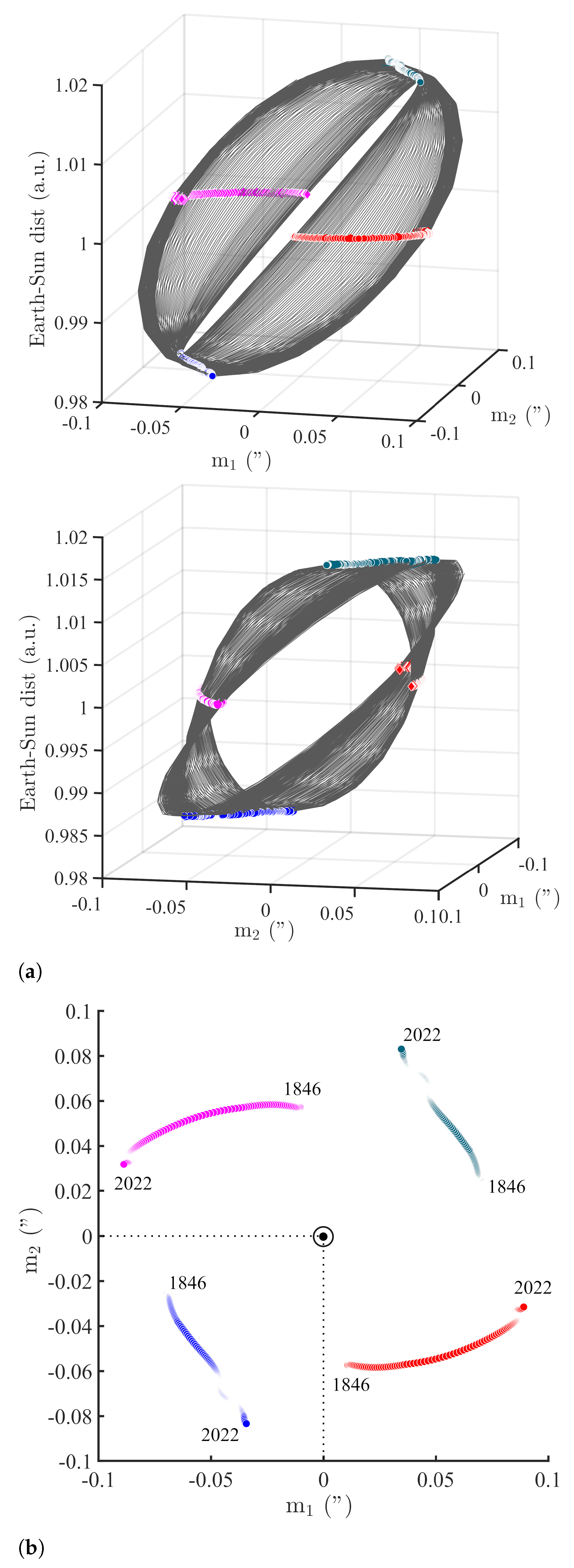
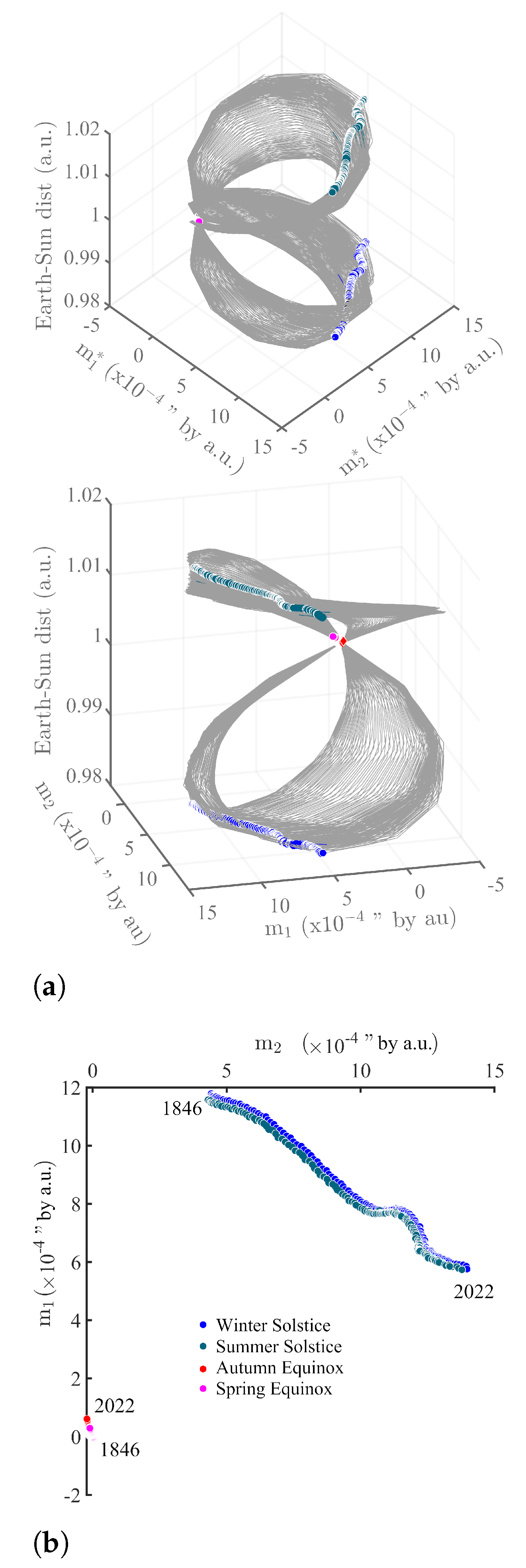
4. The Lissajous Diagrams

The main points in space that can be used to monitor the precession of an elliptical orbit are the solstices and equinoxes. The fixed dates of their occurrences are 21 December for the Winter solstice, 21 March for the Spring equinox, 21 June for the Summer solstice, and 23 September for the Fall equinox. Since the legal and astronomical calendars are not exactly the same, this entails an error on their positions that can be estimated. The variations of these positions are actually very small: the perimeter of the Earth’s orbit being close to 6.28 astronomical units (a.u.), the 21 December positions are at a distance of 0.98412 ± 3.46 × 10${}^{-5}$ a.u., that is an error of 5.5 × 10${}^{-4}$ between 1844 and 2022. The error is 5.8 × 10${}^{-4}$ for the other solstice and close to 7.9 × 10${}^{-4}$ and 8.7 × 10${}^{-4}$ for the two equinoxes.

To built our Lissajous diagrams, we first extracted the annual component of pole motion. In Figure 4 we show this forced component.

Figure 5a shows the evolution of the trajectories of Figure 4a as a function of Sun–Earth distance (ephemerids), that is in other words as a function of time. We call these by analogy to Lissajous orbits in astronomy “Lissajous diagrams”. The Lissajous diagram of ($m_1$, $m_2$) is shown in two perspectives in order to gain some insight on its topology. The locations of the four remarkable points (equinoxes and solstices) are shown in four different colors (the same are used throughout of the paper). We can see that the closer the Earth is to the Sun, the more the rotation axis straightens; the farther it is, the larger the amplitudes of motions and the flatter the rotation axis, i.e., the larger its declination (see also Figure 5b). Note that the “fixed dates” of equinoxes and solstices appear to drift as a function of time.

The conservation of momentum of the orbiting planet implies that its areolar velocity is constant (the areolar velocity is the area spanned by the vector radius—the Sun to Earth vector-per unit time). As a consequence of this “law of areas”, the orbital velocity varies from a maximum of 30.29 km/s at perihelion to a minimum of 29.29 km/s at aphelion. As explicitly stated by [7,8,47,48] long ago, and recently re-emphasized by [5,38,49], the iSSA annual component of polar motion ($m_1$, $m_2$) is controlled by variations in Sun–Earth distance $d_{SE}$.

In order to emphasize the relative amplitudes of the drift and the butterfly-like shape of the diagram, we have actually multiplied ($m_1$, $m_2$) by the centered value $d_{SE}^{*}=d_{SE}-mean\left(d_{SE}\right)$. This also makes it clear that the drift of solstices is larger than that of equinoxes. Figure 6a shows the Lissajous diagram equivalent to that in Figure 5a for the couple ($m_1^{*}$,$m_2^{*}$). The Lissajous diagrams of Figure 6a represent the geodesic evolution of Kepler areas.

One sees clearly in Figure 6a that polar motion reaches a minimum at the equinoxes (red and orange dots) when solar attraction is the weakest, and a maximum at the solstices (green and blue dots) when the Sun, Earth and focus of the ellipse are aligned. We shall see below that the same applies to lod.

These results actually require another small correction, in relation with Kepler’s second law. The conservation of momentum of the orbiting planet implies that its areolar velocity is constant (the areolar velocity is the area spanned by the vector radius—the Sun to Earth vector—per unit time). As a consequence of this “law of areas”, the orbital velocity varies from a maximum of 30.29 km/s at perihelion to a minimum of 29.29 km/s at aphelion. We introduce new more physical variables by multiplying the polar motion coordinates by the Sun–Earth distance $d_{SE}$:

$$m_1^{*}=m_1\times d_{SE},m_2^{*}=m_2\times d_{SE}$$

We display the drift of the four reference points (solstices and equinoxes) in the ($m_1^{*}$, $m_2^{*}$.) plane in Figure 6b. The time evolution of the separate coordinates $m_1^{*}$ and $m_2^{*}$ for the solstices are shown in Figure 7a,b.

5. Discussion

Milanković [3] knew that eccentricity, precession and obliquity evolve slowly in time leading to a transition from a warmer to a cooler climate every 11,000 year (the period of precession of equinoxes being the shortest). Figure 5, Figure 6 and Figure 7 show that one cannot consider that either the Sun–Earth distance or the hour angle, or the declination, or the daily variation are constant, contrary to what was done by [3]. Both polar motions and length of day are affected by their position on the elliptical orbit, on rather short periods on the order of less than 10 year up to 1 century or more. The data shown in the present paper demonstrate that parameters in Equation (1) evolve in time over these shorter time scales. They may, therefore, imply some forcing of climate on these same time scales.

Figure 1a illustrates the differences between five data sets that were supposed when they were compiled to represent the same physical (or quasi-physical) datum, that is mean global surface temperature anomaly. Figure 8a displays the iSSA trends (component 1) of the five HadCrut temperature data sets introduced in Section 2.1. The median of the five curves is shown as an inset in Figure 8a. Figure 8b,c represent the two other major iSSA components of global mean temperature anomaly, the annual and 60 year oscillations. The frequencies of the five series are consistent except for the modulated amplitudes of the annual components (Figure 8b), which is puzzling.

In Figure 9, we superimpose the time evolution of the winter (blue) and summer (green) solstices for component $m_1^{*}$ from Figure 7a and the first iSSA component (trend) of the median of the five HadCrut Center temperature series (red) from Figure 8a (note: We have simplified the discussion by using only the m1 polar motion component, the one most clearly linked to the pole’s inclination). With some familiarity with global temperature curves, one can recognize some common features with the evolution of the solstices [31]. Based on the annual oscillations of the full polar motion ($m_1$, $m_2$ and lod), we have seen that the celestial positions of solstices moved significantly in the past 180 years. To our knowledge, this is the first time one evidences in the observational data what [23] called the apparent precession of solstices (that is seen from Earth) and that Milanković (part 2, chapter 2) worked on, but on much longer time periods of millions of years. We recalled in the introduction the basic equation from Milanković’s thesis (1920) that links time variations of heat received at a given location on Earth to solar insolation, known functions of the location coordinates, solar declination and hour angle, with an inverse square dependence on the Sun–Earth distance. We can let W play the role of the heat/energy term in Equation (1). The goal is to translate the drift of solstices as a function of distance to the Sun into the geometrical insolation theory of [3].

6. Conclusions

The Earth’s revolution is modified by changes in inclination of its rotation axis, principally due to the actions of the Moon and Sun. Despite the fact that the gravity field is central, the Earth’s trajectory is not closed and the equinoxes drift (by a little less than one minute of arc per year, that is a precession period of some 26,000 year—[23]). For d’Alembert, Lagrange, Laplace and Poincaré, who based their reasoning on the action of torques, as in a top, changes in polar motion and revolution are coupled (through the Liouville–Euler system of equations). Re-organization of Earth’s fluid envelopes follows. For Newton, who gives a central role to the inertia tensor, planetary bodies attract (or repel) the oceans (and atmospheres) and this re-organization of masses modifies the rotation axis.

Milanković (cf. [3], p. 221) argued that the shortest precession period of perihelion (for us solstices) is 20,700 Julian years and that the consequence of this precession is that the summer solstice in one hemisphere takes place alternately every 11,000 year at perihelion (a warmer summer) and at aphelion (a cooler summer). The difference in insolation between maximum and minimum is a function of eccentricity. Milanković assumed that the planetary distances to the Sun and the solar ephemerids are constant. There are now observations that allow one to drop the hypothesis that Sun–Earth distance, the Sun’s declination and hourly angle (Equation (1)) are constant. Thus, we can evaluate whether changes in the position of the rotation axis affect, for instance, atmospheric temperature, that is the main parameter in Milanković theory of climate.

Both the apparent drift of solstices of Earth around the Sun and the global mean temperature exhibit a strong 60 year oscillation. In the present paper, we have confirmed the finding of a strong iSSA component with 60 year period in global temperatures and in the drift of solstices (Figure 8c and Figure 10), hence the rotation axis, that has already been encountered in [33,34,35,50,51,52,53,54,55,56,57,58,59].

In pursuit of this goal, we obtained the Sun’s ephemerids from 1846 to the present from Institut de Mécanique Céleste et du Calcul des Ephémérides (data set EOP C01 IAU1980). The motions of the rotation pole and variations in rotation velocity were taken from the International Earth Rotation Reference Systems Service. They consist in the couple of coordinates ($m_1$, $m_2$) of motion of the rotation pole PM and the length of day lod. We used the semi-annual lod data provided by [37] for the period 1832–1997, combined with the IERS data, resulting in a mean curve between 1832 and 2022 (Figure 2c). For the mean global temperatures, we used five HadCrut data series from the Hadley Center for Climate Prediction and Research in order to estimate the consistence of the data. There are rather significant differences between the five data series, resulting in differences in the dominant spectral peak that shifts from 60 to 80 year.

We have submitted the time series for the rotation, temperature and ephemeris to iterative Singular Spectrum Analysis (iSSA), a method which we have used extensively in a number of recent studies ([12,31,39]). We have checked that the results obtained with iSSA match those obtained with the more common method of continuous wavelets that is widely used in the literature.

The main points in space that can be used to monitor the precession of an elliptical orbit are the solstices and equinoxes. The legal and astronomical calendars not being exactly the same, this entails a very small error on their positions (relative variations of their positions between 5 and 9 × 10${}^{-4}$) between 1844 and 2022.

Figure 5a shows the evolution of the locations of the equinoxes and solstices trajectories as a function of Sun–Earth distance (we call these “Lissajous diagrams”). The closer the Earth is to the Sun, the more the rotation axis straightens; the farther it is, the larger the amplitudes of motions and the flatter the rotation axis. The “fixed dates” of equinoxes and solstices actually drift as a function of time. In order to emphasize the relative amplitudes of the drift and the butterfly-like shape of the Lissajous diagram, we have actually multiplied ($m_1,m_2$) by the centered value $d_{SE}^{*}=d_{SE}–mean\left(d_{SE}\right)$, yielding ($m_1^{*}$, $m_2^{*}$). This also makes it clear that the drift of solstices is larger than that of equinoxes. Polar motion reaches a minimum at the equinoxes when solar attraction is the weakest, and a maximum at the solstices when the Sun, Earth and focus of the ellipse are aligned.

Both polar motions and length of day are affected by their position on the elliptical orbit, on rather short periods on the order of less than 10 year up to 1 to a few centuries. The parameters in Equation (1) evolve over these time scales. Some forcing of climate on these same time scales may be expected.

Despite differences between the five HadCrut temperature data sets, the median of the first iSSA component (trend) appears to be representative (Figure 8a). The two other major iSSA components of the five global mean temperature anomaly series, the annual and 60 year oscillations, are consistent; the modulated amplitudes of the annual components do not agree as well (Figure 8b).

We have superimposed the time evolution of the winter and summer solstices for component $m_1^{*}$ and the first iSSA component (trend) of the median of the five HadCrut Center temperature series (Figure 9). Based on the annual oscillations of the full polar motion (m1, m2 and lod), we have shown that the celestial positions of solstices moved significantly in the past 180 years. To our knowledge, this is the first time one evidences in the observational data what d’Alembert (1749) called the apparent precession of solstices (that is seen from Earth) and that Milanković ([3]), part 2, chapter 2) worked on, but on much longer time periods of millions of years.

One can recognize in Figure 9 some common features between the evolution of the solstices and the trend of temperatures. We recalled in the introduction the basic equation from Milanković’s thesis ([3]) that links time variations of heat W received at a given location on Earth to solar insolation, known functions of the location coordinates, solar declination and hour angle, with an inverse square dependence on the Sun–Earth distance. We translate the drift of solstices as a function of distance to the Sun into the geometrical insolation theory of Milankovic (1920). Both the apparent drift of solstices of Earth around the Sun and the global mean temperature exhibit a strong 60 year oscillation (Figure 8c and Figure 10).

It may seem that we navigate between two pitfalls: remembering that correlation does not imply causality at the risk of discounting a potentially interesting relationship or accepting the causality when it does not exist, at the risk of pursuing a non existent theory. We do acknowledge that one should not jump too fast to conclusions, yet the probability of a chance coincidence in Figure 10 appears very low. Correlation certainly does not imply causality when there is no accompanying model. But in the case studied in this paper, Equation (1) can be considered as a model that is widely accepted. Equation (1) links the time derivative of insolation with the inverse square of the Sun–Earth distance. In Figure 10, shifting the inverse square of the 60 year iSSA drift of solstices by 15 years with respect to the first derivative of the 60 year iSSA trend of temperature, that is exactly a quadrature in time, puts the two curves in quasi-exact agreement. This is a case of agreement between observations and a mathematical formulation. This new finding joins a host of recent results that argue in the same direction [17]; the hypothesis proposes that a forcing by the giant Jovian planets is exerted on a vast number of solar and terrestrial phenomena, including, as shown in this paper, global surface temperature. This forcing induces a number of responses from the Earth’s rotation axis, hence on climate at many time scales. This is a sort of extension of the Milankovic theory of climate to a range of periods that are much shorter than the ∼20,000 year minimum often associated with this theory.

References

1. Agassiz, L. Discours sur les Glaciers; Assemblée de la Société Helvétique des Sciences Naturelles: Neuchâtel, Switzerland, 1837. [Google Scholar]
2. Adhémar, J.A. Sur les Révolutions de la mer, Déluges Périodiques; Lacroix-Comon: Paris, France, 1860; Volume 1. [Google Scholar]
3. Milanković, M. Théorie Mathématique des phéNomènes Thermiques Produits par la Radiation Solaire; Faculté des Sciences de l’Université de Belgrade, Gauthier-Villard Edition: Paris, France, 1920. [Google Scholar]
4. Laskar, J.; Robutel, P.; Joutel, F.; Gastineau, M.; Correia, A.C.M.; Levrard, B. A long-term numerical solution for the insolation quantities of the Earth. Astron. Astrophys. 2004, 428, 261–285. [Google Scholar] [CrossRef] [Green Version]
5. Lopes, F.; Zuddas, P.; Courtillot, V.; Le Mouël, J.L.; Boulé, J.B.; Maineult, A.; Gèze, M. Milankovic Pseudo-cycles Recorded in Sediments and Ice Cores Extracted by Singular Spectrum Analysis. Clim. Past Discuss. 2021, 1–17. [Google Scholar] [CrossRef]
6. Lisiecki, L.E.; Raymo, M.E. A Pliocene-Pleistocene stack of 57 globally distributed benthic δ18O records. Paleoceanography 2005, 20, 565. [Google Scholar] [CrossRef] [Green Version]
7. Laplace, P.S. Traité de Mécanique Céleste; l’Imprimeri e de Crapelet: Paris, France, 1799. [Google Scholar]
8. Poincaré, H. Les Méthodes Nouvelles de la Mécanique Céleste; Gauthier-Villars: Paris, France, 1893. [Google Scholar]
9. Sidorenkov, N.S. Physics of Earth’s rotational instabilities. Astrono. Astrophy. Trans. J. Eurasian Astron. Soc. 2005, 24, 425–439. [Google Scholar] [CrossRef]
10. Sidorenkov, N.S. The Interaction Between Earth’s Rotation and Geophysical Processes; John Wiley & Sons: Berlin, Germany, 2009; ISBN 978-3-527-62772-1. [Google Scholar]
11. Ray, R.D.; Erofeeva, S.Y. Long-period tidal variations in the length of day. J. Geophys. Res. Solid Earth 2014, 119, 1498–1509. [Google Scholar] [CrossRef]
12. Le Mouël, J.L.; Lopes, F.; Courtillot, V.; Gibert, D. On forcings of length of day changes: From 9-day to 18.6-year oscillations. Phys. Earth Planet. Inter. 2019, 292, 1–11. [Google Scholar] [CrossRef]
13. Laskar, J.; Joutel, F.; Boudin, F. Orbital, precessional, and insolation quantities for the Earth from-20 Myr to+ 10 Myr. Astron. Astrophys. 1993, 270, 522–533. [Google Scholar]
14. Mörth, H.T.; Schlamminger, L. Planetary Motion, Sunspots and Climate, Solar-Terrestrial Influences on Weather and Climate; Springer: Dordrecht, The Netherlands, 1979; Volume 193. [Google Scholar]
15. Courtillot, V.; Lopes, F.; Le Mouël, J.L. On the prediction of solar cycles. Sol. Phys. 2021, 296, 21. [Google Scholar] [CrossRef]
16. Lopes, F.; Le Mouël, J.L.; Courtillot, V.; Gibert, D. On the shoulders of Laplace. Phys. Earth Planet. Inter. 2021, 316, 106693. [Google Scholar] [CrossRef]
17. Bank, M.J.; Scafetta, N. Scaling, mirror symmetries and musical consonances among the distances of the planets of the solar system. Front. Astron. Space Sci. 2022, 8, 758184. [Google Scholar] [CrossRef]
18. Scafetta, N.; Milani, F.; Bianchini, A. A 60-year cycle in the Meteorite fall frequency suggests a possible interplanetary dust forcing of the Earth’s climate driven by planetary oscillations. Geophys. Res. Lett. 2022, 47, e2020GL089954. [Google Scholar] [CrossRef]
19. Yndestad, H. Jovian Planets and Lunar Nodal Cycles in the Earth’s Climate Variability. Front. Astron. Space Sci. 2022, 9, 839794. [Google Scholar] [CrossRef]
20. Orgeira, M.J.; Velasco Herrera, V.M.; Cappellotto, L.; Compagnucci, R.H. Statistical analysis of the connection between geomagnetic field reversal, a supernova, and climate change during the Plio–Pleistocene transition. Int. J. Earth Sci. 2022, 111, 1357–1372. [Google Scholar] [CrossRef]
21. Courtillot, V.; Gallet, Y.; Le Mouël, J.L.; Fluteau, F.; Genevey, A. Are there connections between the Earth’s magnetic field and climate? Earth Planet. Sci. Lett. 2007, 253, 328–339. [Google Scholar] [CrossRef]
22. Landau, L.; Lifchitz, E. Physic Theory, Part 2 Mecanic; Mir Edition: Moscow, Russia, 1964. [Google Scholar]
23. d’Alembert, J.L.R. Recherches sur la Précession des Equinoxes: Et sur la Nutation de L’axe de la terre, Dans le systêMe Newtonien; chez David l’aîné: Paris, France, 1749. [Google Scholar]
24. Schwarzschild, K. Über das Gravitationsfeld einer Kugel aus inkompressibler Flüssigkeit nach der Einsteinschen Theorie. Sitzungsberichte der KöNiglich PreußIschen Akad. der Wiss. zu Berl. 1916, 23, 424–434. [Google Scholar]
25. Lense, J.; Thirring, H. On the influence of the proper rotation of a central body on the motion of the planets and the moon, according to Einstein’s theory of gravitation. Z. Für Phys. 1918, 19, 41. [Google Scholar]
26. Rayner, N.A.; Horton, E.B.; Parker, D.E.; Folland, C.K.; Hackett, R.B. Version 2.2 of the Global Sea-Ice and Sea Surface Temperature Dataset, 1903–1994; Climate Research Technical Note 74; Hadley Centre, U.K. Meteorological Office: Exeter, UK, 1996.
27. Rayner, N.A.; Parker, D.E.; Horton, E.B.; Folland, C.K.; Alexander, L.V.; Rowell, D.P.; Kent, E.C.; Kaplan, A. Globally complete analyses of sea surface temperature, sea ice and night marine air temperature, 1871-02000. J. Geophys. Res. 2003, 108, 4407. [Google Scholar] [CrossRef] [Green Version]
28. Brohan, P.; Kennedy, J.J.; Harris, I.; Tett, S.F.B.; Jones, P.D. Uncertainty estimates in regional and global observed temperature changes: A new dataset from 1850. J. Geophys. Res. 2006, 111, D1210. [Google Scholar] [CrossRef] [Green Version]
29. Osborn, T.J.; Jones, P.D. The CRUTEM4 land-surface air temperature data set: Construction, previous versions and dissemination via Google Earth. Earth Syst. Sci. Data 2014, 6, 61–68. [Google Scholar] [CrossRef] [Green Version]
30. Osborn, T.J.; Jones, P.D.; Lister, D.H.; Morice, C.P.; Simpson, I.R.; Winn, J.P.; Hogan, E.; Harris, I.C. Land surface air temperature variations across the globe updated to 2019: The CRUTEM5 dataset. J. Geophys. Res. Atmos. 2021, 126, e2019JD032352. [Google Scholar] [CrossRef]
31. Le Mouël, J.L.; Lopes, F.; Courtillot, V. Characteristic time scales of decadal to centennial changes in global surface temperatures over the past 150 years. Earth Space Sci. 2020, 7, e2019EA000671. [Google Scholar] [CrossRef] [Green Version]
32. Courtillot, V.; Le Mouël, J.L.; Kossobokov, K.; Gibert, D.; Lopes, F. Multi-Decadal Trends of Global Surface Temperature: A Broken Line with Alternating 30 Year Linear Segments? NPJ Clim. Atmos. Sci. 2013, 3, 34080. [Google Scholar] [CrossRef] [Green Version]
33. Mazzarella, A.; Scafetta, N. Evidences for a quasi 60-year North Atlantic Oscillation since 1700 and its meaning for global climate change. Theor. Appl. Climatol. 2012, 107, 599–609. [Google Scholar] [CrossRef]
34. Gervais, F. Anthropogenic CO2 warming challenged by 60-year cycle. Earth-Sci. Rev 2016, 155, 129–135. [Google Scholar] [CrossRef]
35. Veretenenko, S.; Ogurtsov, M. Manifestation and possible reasons of ∼60-year oscillations in solar-atmospheric links. Adv. Space Res. 2019, 64, 104–116. [Google Scholar] [CrossRef]
36. Lambeck, K. The Earth’s Variable Rotation: Geophysical Causes and Consequences; Cambridge University Press: New York, NY, USA, 2005. [Google Scholar]
37. Stephenson, F.R.; Morrison, L.V. Long-term changes in the rotation of the Earth: 700 BC to AD 1980. Philos. Trans. R. Soc. A 1984, 313, 47–70. [Google Scholar]
38. Lopes, F.; Courtillot, V.; Gibert, D.; Le Mouël, J.-L. On Two Formulations of Polar Motion and Identification of Its Sources. Geosciences 2022, 12, 398. [Google Scholar] [CrossRef]
39. Le Mouël, J.L.; Lopes, F.; Courtillot, V. Singular spectral analysis of the aa and Dst geomagnetic indices. J. Geophys. Res. Space Phys. 2019, 124, 6403–6417. [Google Scholar] [CrossRef]
40. Le Mouël, J.L.; Lopes, F.; Courtillot, V. Solar turbulence from sunspot records. Mon. Notices Royal Astron. Soc. 2020, 492, 1416–1420. [Google Scholar] [CrossRef]
41. Golyandina, N.; Zhigljavsky, A. Singular Spectrum Analysis; Springer: Berlin/Heidelberg, Germany, 2013. [Google Scholar]
42. Lemmerling, P.; Van Huffel, S. Analysis of the structured total least squares problem for Hankel/Toeplitz matrices. Numer. Algorithms 2001, 27, 89–114. [Google Scholar] [CrossRef]
43. Golub, G.H.; Reinsch, C. Singular Value Decomposition and Least Squares Solutions; Linear Algebra; Springer: Berlin/Heidelberg, Germany, 1971; pp. 134–151. [Google Scholar]
44. Gibert, D.; Holschneider, M.; Le Mouël, J.L. Wavelet analysis of the Chandler wobble. J. Geophys. Res. 1998, 103, 27069–27089. [Google Scholar] [CrossRef]
45. Grossmann, A.; Morlet, J. Decomposition of Hardy functions into square integrable wavelets of constant shape. SIAM J. Math. Anal. 1984, 15, 723–736. [Google Scholar] [CrossRef] [Green Version]
46. Auger, F.; Flandrin, P. Improving the readability of time-frequency and time-scale representations by the reassignment method. IEEE Trans. Signal Process. 1995, 43, 1068–1089. [Google Scholar] [CrossRef] [Green Version]
47. Lagrange, J.L. Oeuvres Complètes, t. V; Gauthier-Villars: Paris, France, 1870; Volume 125. [Google Scholar]
48. Lagrange, J.L. Oeuvres Complètes, t. V; Gauthier-Villars: Paris, France, 1870; Volume 211. [Google Scholar]
49. Courtillot, V.; Le Mouël, J.-L.; Lopes, F.; Gibert, D. On the Nature and Origin of Atmospheric Annual and Semi-Annual Oscillations. Atmosphere 2022, 13, 1907. [Google Scholar] [CrossRef]
50. Lau, K.M.; Weng, H. Climate signal detection using wavelet transform: How to make a time series sing. Bull. Am. Meteorol. Soc. 1995, 76, 2391–2402. [Google Scholar] [CrossRef]
51. Chen, Z.; Grasby, S.E.; Osadetz, K.G. Relation between climate variability and groundwater levels in the upper carbonate aquifer, southern Manitoba, Canada. J. Hydrol. 2004, 290, 43–62. [Google Scholar] [CrossRef]
52. Groot, M.H.M.; Lourens, L.J.; Hooghiemstra, H.; Vriend, M.; Berrio, J.C.; Tuenter, E.; Van der Plicht, J.; Van Geel, B.; Ziegler, M.; Weber, S.L.; et al. Ultra-high resolution pollen record from the northern Andes reveals rapid shifts in montane climates within the last two glacial cycles. Clim. Past 2011, 7, 299–316. [Google Scholar] [CrossRef] [Green Version]
53. Sello, S. On the sixty-year periodicity in climate and astronomical series. arXiv 2011, arXiv:1105.3885. [Google Scholar]
54. Zheng, W.; Jing, W. Analysis on global temperature anomalies from 1880 based on genetic algorithm. Quat. Sci. 2011, 31, 66–72. [Google Scholar] [CrossRef]
55. Chambers, D.P.; Merrifield, M.A.; Nerem, R.S. Is there a 60-year oscillation in global mean sea level? Geophys. Res. Lett. 2012, 39, L18607. [Google Scholar] [CrossRef] [Green Version]
56. Scafetta, N. A shared frequency set between the historical mid-latitude aurora records and the global surface temperature. J. Atmos. Sol. Terr. Phys. 2012, 74, 145–163. [Google Scholar] [CrossRef] [Green Version]
57. Parker, A. Natural oscillations and trends in long-term tide gauge records from the Pacific. Pattern Recogn. Phys. 2013, 1, 1–13. [Google Scholar] [CrossRef]
58. D’Aleo, J.S. Solar changes and the climate. In Evidence based Climate Science; Elsevier: Amsterdam, The Netherlands, 2016; pp. 263–282. [Google Scholar]
59. Pan, H.; Lv, X. Is there a quasi 60-year oscillation in global tides? Cont. Shelf Res. 2021, 222, 104433. [Google Scholar] [CrossRef]
Figure 1. The five HadCrut mean global temperatures since 1850. (a) The five mean global temperature data sets HadCrut1 to HadCrut5 from 1850 to the present maintained by the Hadley Center for Climate Prediction and Research (see text). (b) The 5 Fourier spectra of the 5 data sets in Figure 1a.
Geosciences 12 00448 g001
Figure 2. Pole motion and length of day from IERS data. (a) Evolution of the couple ( m 1 , m 2 ) since 1846 (IERS data). (b) Evolution of lod since 1962 (IERS data). (c) Black curve: lod semi-annual data since 1832 (from [37]); gray: daily lod data since 1962 from IERS; red curve: The median of the trend for these two combined data sets.
Geosciences 12 00448 g002aGeosciences 12 00448 g002b
Figure 3. Extraction of oscillatory component by continues wavelet transform: an example. (a) Black curve: annual component of lod extracted by the method of continuous wavelets; Red curve: annual component of lod extracted by the iSSA method. (b) Scalogram of lod since 1962. The wavelet cone of influence is symbolized by the gray area. The red dashed lines enclose the wavelet coefficients corresponding to the 1 year period.
Geosciences 12 00448 g003
Figure 4. Annual components extracted from pole path and lod. (a) The annual couple ( m 1 , m 2 ) of polar motion coordinates extracted by iSSA. (b) The annual component of lod extracted by iSSA.
Geosciences 12 00448 g004
Figure 5. Drift of equinoxes and solstices since 1846. (a) Lissajous diagram for the couple of rotation pole motion coordinates ( m 1 , m 2 ) as they vary with Sun–Earth distance, i.e., as a function of time. (b) Projection of the drift of equinoxes and solstices from 1846 to the present in the ( m 1 , m 2 ) plane.
Geosciences 12 00448 g005
Figure 6. Drift of equinoxes and solstices since 1846 with the new parameters m 1 * and m 2 * . (a) Lissajous diagram for the couple of coordinates ( m 1 * , m 2 * ) as they vary with Sun-Earth distance, i.e., as a function of time. (b) Projection of the drift of equinoxes and solstices from 1846 to the present in the ( m 1 * , m 2 * ) plane.
Geosciences 12 00448 g006
Figure 7. Time evolution of winter and summer solstices. (a) Time evolution of winter and summer solstices for component m 1 * . (b) Time evolution of winter and summer solstices for component m 2 * .
Geosciences 12 00448 g007
Figure 8. Trend, one year and sixty years components extracted from HadCrut curves. (a) The first iSSA components (trends) of the five HadCrut Center temperature series introduced in Section 2.1, and their median shown in black among the 5 trends and alone above as an inset. (b) Annual iSSA components of the same series as in Figure 8a. (c) Sixty year iSSA components of the same series as in Figure 8a.
Geosciences 12 00448 g008aGeosciences 12 00448 g008b
Figure 9. Superposition of the time evolution of the winter (blue curve) and summer (green curve) solstices for component m 1 * from Figure 7a and the first iSSA component (trend) of the median of the five HadCrut Center temperature series from Figure 8a (red curve).
Geosciences 12 00448 g009
Figure 10. (top) In red, the derivative of the iSSA trend of temperature; in green and blue, the inverse square of the drift of solstices. (bottom) A phase quadrature has been applied to the solstices curves above, that is a backward translation of 15 year (=60 years/4).
Geosciences 12 00448 g010
Publisher’s Note: MDPI stays neutral with regard to jurisdictional claims in published maps and institutional affiliations.