
Comparison between Calculation and Measurement of Total Sediment Load: Application to Streams of NE Greece


1
Department of Civil Engineering, Democritus University of Thrace, 67100 Xanthi, Greece
2
Faculty of Science and Technology, Free University of Bozen-Bolzano, 39100 Bolzano, Italy
*
Author to whom correspondence should be addressed.
Geosciences 2022, 12(2), 91; https://0-doi-org.brum.beds.ac.uk/10.3390/geosciences12020091
Submission received: 6 December 2021
/
Revised: 29 January 2022
/
Accepted: 10 February 2022
/
Published: 17 February 2022
(This article belongs to the Special Issue Recent Advances on Sediment Transport and River Morphodynamics)
Abstract
:Sediment transport and stream discharge are two of the natural procedures which affect the hydromorphological profile of a watercourse. Measurements of water discharge, bed load transport rate and suspended sediment concentration were conducted in Kosynthos River and Kimmeria Torrent –two intermittent streams– in north-eastern Greece. The total sediment concentration was calculated, in both streams, by means of various nonlinear regression equations and by means of the formulas of Yang, after calibrating the coefficients of the formulas. In the computations according to the Yang formulas, two different states were examined regarding the incipient motion: one considering and one disregarding the critical conditions. The results obtained from Yang’s multiple regression-derived equations had a better fit compared to the original equations and were acceptable in both cases. Ultimately, two counterparts of Yang’s stream sediment transport formulas were constructed and made available to the readership. The comparison between the calculated and measured total sediment concentrations was achieved by means of several statistical criteria. The results indicate that the modified formulas of Yang can be successfully used for the determination of the total sediment concentration in Kosynthos River and Kimmeria Torrent.
1. Introduction
One of the long-lasting problems hydraulic engineers are faced with is understanding and modeling the processes that govern sediment transport in streams. The difficulty in solving this problem lies in the complexity of the physical processes that describe it [1] and the variety of the types of the existing watercourses. On the other hand, sediment monitoring stations are very sparse, and hence the bulk of streams worldwide remains ungauged. In addition, the estimation of sediment discharge by conventional measurement methods is expensive and labor intensive, and therefore, alternative, less expensive approaches to predict their background processes are desirable [2,3].
Langbein and Iseri [4] introduced a classification of rivers as “perennial”, “intermittent” and “ephemeral”, based on their relation to time and seasonality. Perennial rivers have a continuous flow throughout the year, intermittent or seasonal rivers flow at specific wet seasons of the year when there are sufficient water resources, while the flow of ephemeral streams emanates only from surface runoff or snowmelt. Williamson et al. [5] took this one step further by developing a standardized protocol based not only on field-based procedures, but also on regionally calibrated hydrologic models, to classify ephemeral, intermittent, and perennial streams in the area of Kentucky, USA. Sefton et al. [6] created heat maps using spatial analysis in order to classify the hydrological state of headwaters of the Thames River basin in the UK.
Greece has big rivers (e.g., Evros, Nestos, and Strymonas) which drain the southern part of the Balkan Peninsula and convey large volumes of water and sediment. Situated, however, in the Mediterranean semi-arid climate zone, Greece is teeming with ephemeral streams in all regions of the country. There is a variety of watercourses which are characterized by the instability of flow conditions and hydrological fluctuations.
The scientific interest focuses on studying the sediment transport processes and monitoring, modeling and predicting the sediment loads. Apart from theory and modeling, sediment research has been focusing on creating sediment transport databases, either by conducting field measurements or by gathering data from the literature [7,8], in order to quantify the sediment transport of different types of streams. In this direction, the Section of Hydraulic Engineering, Civil Engineering Department, Democritus University of Thrace, has been conducting measurements of the bed load transport rate and suspended sediment concentration at the basin outlet of all three different types of rivers of north-eastern Greece, such as Nestos River (perennial), Kosynthos River, Kimmeria Torrent (intermittent) and a few ephemeral streams.
There is a great variety of sediment transport formulas which can be applied to watercourses, depending on the type of the stream, the hydraulic conditions and the available measurements. Apart from the well-known equations for sediment transport [9,10,11,12,13,14], there is a large number of formulas developed based on various natural rivers or laboratory flumes which can be applied in similar case studies [15].
The data-based calibrated formulas result from applying different types of regression depending on the type of the original formula. In that way, counterparts of established stream sediment formulas are constructed by minimizing the sum of square errors, using linear or nonlinear regression equations, or even by using fuzzy regression equations [8]. Regression analysis has been extensively employed in the literature to either derive sediment transport/concentration equations as a function of hydraulic or hydrometeorological parameters or to adjust existing well-known sediment transport models to environments with specific features different from the ones they were created for. Based on measured sediment data from the Yellow River, Wu et al. [16] modified Yang’s (1996) model [17] by means of regression analysis, resulting in an equation form similar to Yang’s (1979) model [18]. Baniya et al. [19] derived a nonlinear regression equation for annual suspended sediment yield as a function of flow discharge for Kali Gandaki River in Nepal. Ulke et al. [20] satisfactorily generated daily suspended sediment load data for a missing record period in Gediz River in Turkey by means of multiple linear and nonlinear regressions using the discharge and precipitation of the target day and one day prior to the target day as predictors.
Nonlinear regression equations between bed load transport rate and stream flow rate, as well as between suspended load transport rate and stream flow rate have been established for the outlets of Nestos River basin [21], Kosynthos River basin [22,23] and Kimmeria Torrent basin [23]. Based on the available data for each basin, various polynomial, exponential and hyperbolic regression curves were derived in order to estimate bed load, suspended load and total load transport rates. Metallinos and Hrissanthou [23] used nonlinear regression equations to determine the sediment transport of a stream as a function of hydrologic parameters, such as stream discharge, rainfall depth and rainfall intensity.
Avgeris et al. [24] applied Yang’s formulas, a hydraulic approach to the problem of sediment transport, in which the leading parameter is the unit stream power. In the present study, Yang’s formulas are also used, as they are best implemented in this type of available datum. The objective of this study is to redetermine the arithmetic coefficients of the total sediment transport rate formulas of Yang based on field data of Kosynthos River and Kimmeria Torrent, using multiple regressions, and thus create modified equations that will provide substantially more accurate calculations of sediment concentration in these streams. This research also aspires to highlight the significance of customizing and adapting well-established sediment formulas to the specific morphological and flow conditions of rivers and streams. This could effectively tackle the problem of sediment data scarcity.
The results emerging from sediment transport formulas usually differ drastically from each other and from the measured data. Consequently, none of the published sediment transport formulas has gained universal acceptance for confidently predicting sediment transport rates, especially in natural rivers [25].
2. Description of the Study Area
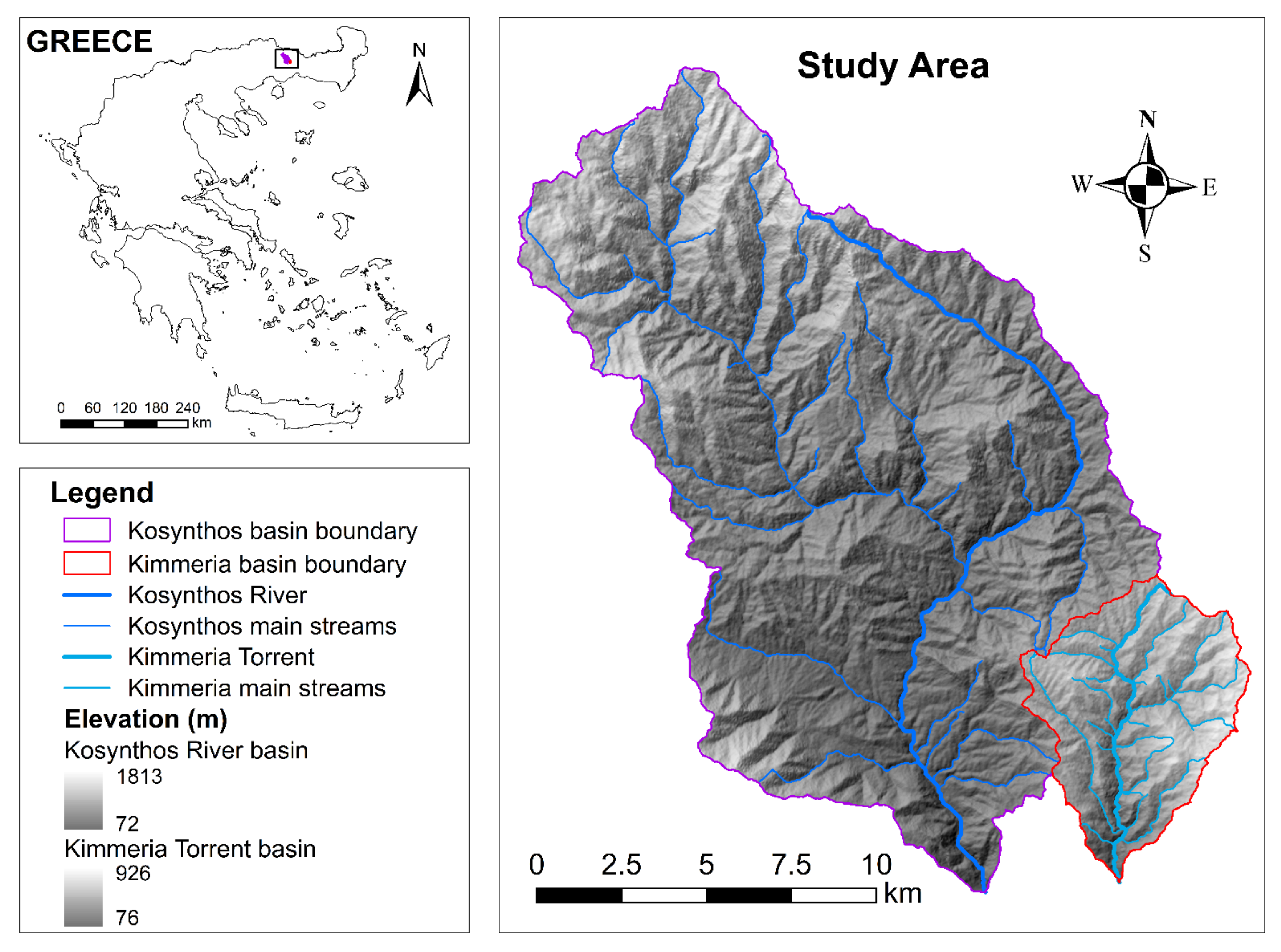
Kosynthos River and Kimmeria Torrent are located in north-eastern Greece (Figure 1), and present similar characteristics regarding their seasonality and physiography. Both basins of the watercourses are considered mainly as rural with a significant coverage of bushy areas, while the mean slope of the main watercourses does not exceed 6%. The average annual temperature is 14 °C and approximately 750 mm of precipitation falls every year. The climate of the study area is characterized as semi-arid, bordering a temperate Mediterranean climate.
The mountainous part of Kosynthos River basin (Figure 1) covers a total area of 237 km2 with elevation ranging from 72 m to 1813 m a.s.l. Kosynthos River flows in a south-eastern course, passing through the city of Xanthi, and its basin outlet is considered at the first Kosynthos’ bridge (inside the city of Xanthi). The length of the main stream that runs the basin is approximately 30.3 km and the mean cross-section width of the stream is 14 m. According to the available measured data, Kosynthos River has an average stream discharge of 1.38 m3 s−1, a mean sediment transport rate of 0.0166 kg s−1 m−1 and a median particle diameter of 0.0009 m.
The mountainous part of Kimmeria Torrent basin (Figure 1) extends to an area of 35 km2 and has an altitude ranging from 76 m to 926 m a.s.l. Kimmeria Torrent runs a course of 11.6 km over the basin’s surface and flows through the village of Kimmeria which lies in the northeast and is a short distance from the city of Xanthi. The basin outlet is located downstream of Kimmeria bridge, and the mean width of the cross-section is 7 m. According to the measurements, Kimmeria Torrent has an average stream discharge of 0.74 m3 s−1, a mean sediment transport rate of 0.0767 kg s−1 m−1 and a median particle diameter of 0.0011 m. It must be noted that the measurements in Kosynthos River and Kimmeria Torrent were conducted on different dates under different flow conditions and are not comparable. The sediment transport rate refers to the total sediment (i.e., bed load and suspended load), while the median particle diameter refers to the bed material which can transition to suspension. Though the median diameter is similar, it can easily be observed that two times lower mean stream discharge, in Kimmeria Torrent, can lead to approximately seven times higher mean sediment discharge compared to Kosynthos River. This can easily be explained by the appreciably smaller geometry of Kimmeria Torrent, which leads to higher flow velocities, even when the discharge is considerably lower.
The end part of the natural basins of Kosynthos River and Kimmeria Torrent is a lowland plain. Kosynthos River flows out to Vistonis Lake, while Kimmeria Torrent is a tributary to Kosynthos River. Figure 1 depicts only the mountainous part of both basins, and the outlets were considered at Kosynthos bridge and Kimmeria bridge, where the measurements were conducted.
3. Data and Methods
A total of 84 datasets of measured stream flow rate, flow depth, bed load transport rate, suspended load transport rate, median particle diameter, and cross-sectional geometry were used. The sum of the measured bed load and suspended load transport rates provides the measured total load transport rate, from which the total sediment concentration can be estimated.
Apart from the measurements, the total sediment concentration was calculated by means of five different ways:
- Three combinations of hydrologic nonlinear regression relationships, based on the paper of Metallinos and Hrissanthou [23], are established and used to predict the total sediment transport load, on the basis of two different sets of field measurements in Kosynthos River and Kimmeria Torrent.
- Yang’s (1973) [11] formula for total sediment concentration.
- Yang’s (1973) [11] formula for total sediment concentration with calibrated coefficients by means of multiple regression based on the field measurements.
- Yang’s (1979) [18] formula for total sediment concentration, without critical conditions for incipient motion.
- Yang’s (1979) [18] formula for total sediment concentration, without critical conditions for incipient motion, with calibrated coefficients by means of multiple regression based on the field measurements.
The efficiency of the methods was evaluated by comparison between calculated and site-measured total sediment concentration.
A crucial stage for stream sediment transport modeling is choosing the proper model among the plethora of total sediment load formulas (e.g., [14,26]). In most cases, the results of these formulas not only differ, but the calculated sediment loads are often of different order of magnitude. This is largely attributed to the empirical or semi-empirical nature of these formulas (and the way they have been derived), which throws their global applicability into question. As stated by Yang et al. [27], the results of sediment transport formulas often differ from each other, as well as from measured data, and some parameters are more effective than others for the estimation of total sediment load.
To evaluate the selection of the right model, we first tested the model of Engelund and Hansen [14], which is also a very well-known formula for total sediment load. The application to both the under-study streams was far from satisfactory resulting in NSE (Nash–Sutcliffe efficiency) values much smaller than the acceptable limits.
The reason for choosing the Yang sediment transport formulas is primarily because they have proven to be efficient in streams similar to the ones of our study. Among some such examples is the application of Yang’s formulas to the main streams of Forggensee Reservoir basin in Austria, Germany [28], to the main streams of Kastoria Lake basin in Greece [29], to the main streams of Kompsatos River basin in Thrace, Greece [30], to the main streams of Yermasoyia Reservoir basin in Cyprus [31], and to the main streams of Nestos River basin in Bulgaria and Greece [32].
3.1. Procedure of Stream Flow Rate and Sediment Transport Rate Measurements
The stream flow rate measurements were conducted by measuring the average flow velocity using a Valeport open-channel flow meter at the outlet of the basins. Each cross-section was divided into sub-sections, the mean velocity was measured at 40% of the flow depth from the bed and then multiplied by the wetted area of the sub-section, resulting in the stream flow rate. The stream discharge of the whole cross-section is the aggregation of the stream discharges of the sub-sections.
The suspended sediment concentration was determined by obtaining a sample of water from the center of the cross-section and subsequently infiltrating it through retention paper filters. The retained mass of the suspended sediment was dried out and divided by the water volume of the sample to define the concentration of the suspended sediment [33].
The bed load transport rate measurements were conducted using a Helley-Smith sampler. The bed load transport rate resulted by dividing the trapped bed load dry mass by the trap width and the duration of the measurement. The median particle diameter of the bed material was determined by means of sieve analysis.
3.2. Calculation of Total Sediment Concentration
3.2.1. Hydrologic Nonlinear Regression Relationships
In a previous study [23], hydrologic nonlinear regression relationships between the sediment transport rate and hydrologic variables were established for Kosynthos River and Kimmeria Torrent. In this paper, a similar attempt has been made, using a larger amount of data, and resulted in the correlation of the following variables for both basins:
- Suspended load transport rate (g s−1) versus stream discharge (m3 s−1).
- Suspended load transport rate (g s−1) versus daily rainfall depth (mm).
- Suspended load transport rate (g s−1) versus rainfall intensity (mm h−1).
- Bed load transport rate (kg s−1 m−1) versus stream discharge (m3 s−1).
Table 1 illustrates the derived equations for Kosynthos River basin and Table 2 the relationships for Kimmeria Torrent basin.
In the present study, 84 sets of measured data were applied to the relationships in Table 1 and Table 2. The comparison is made on the basis of total calculated and measured sediment concentrations and, for this reason, three combinations of the relationships are created:
- Suspended and bed load transport rate versus stream discharge (Combination 1).
- Suspended load transport rate versus daily rainfall depth, and bed load transport rate versus stream discharge (Combination 2).
- Suspended load transport rate versus rainfall intensity, and bed load transport rate versus stream discharge (Combination 3).
By transforming the units of the above-mentioned relationships, we were able to calculate, firstly, the total load transport rate in kg m−1 s−1 for all three combinations, and secondly, the total sediment concentration (ppm by weight).
3.2.2. Yang (1973)
In 1973, Yang derived a formula for the total sediment transport in rivers and streams by applying a multiple regression analysis for 463 sets of data in laboratory flumes [11]:
where cF is the total sediment concentration (ppm by weight); w is the terminal fall velocity of the sediment particles (m s−1); D50 is the median particle diameter (m); ν is the kinematic viscosity of water (m2 s−1); s is the energy slope; u is the mean flow velocity (m s−1); ucr is the critical mean flow velocity (m s−1); and u* is the shear velocity (m s−1). The product us is characterized as unit stream power.
3.2.3. Yang (1979)
In 1979, Yang concluded that the critical unit stream power term in Equation (1) can be neglected without causing much error when the measured sediment concentration is greater than 20 ppm. The simplified unit stream power equation was derived as:
The latter Yang formula was developed based on 1259 sets of laboratory and field data.
4. Results
4.1. Modification of Yang’s Equations on the Basis of Kosynthos River and Kimmeria Torrent Data
In order to redetermine the coefficients of Equation (1), a multiple regression analysis was applied [24]. The logarithmic total sediment concentration, logcF, was set as the dependent variable and the following auxiliary variables x1, x2, x3, x4 and x5 were set as the independent variables:
Then, Yang’s formula can be written as a multiple linear regression equation:
Similarly, if the following auxiliary variables x′1, x′2, x′3, x′4 and x′5 are considered:
Equation (2) can be written as a multiple linear regression equation:
On the basis of Kosynthos River data, the arithmetic coefficients of the original formulas of Yang, Equations (1) and (2), are modified, respectively, as follows:
The corresponding modified formulas of Yang for the Kimmeria Torrent data can be seen in Equations (9) and (10):
In concrete terms, the new arithmetic coefficients of Equations (7)–(10) were determined by means of the conventional least squares regression. Regarding Equations (9) and (10), without the critical condition, it should be noted that the measured total sediment concentrations in Kosynthos River and Kimmeria Torrent do not exceed the threshold of 20 ppm set by Yang [18].
The measured stream flow rate (m3 s−1), the measured total sediment concentration (ppm), as well as the calculated total sediment concentration (ppm), by means of all equations, for Kosynthos River and Kimmeria Torrent, are provided in Table 3 and Table 4, respectively. The double dashes displayed at the aforementioned tables indicate the absence of measured values at the specific type of relationship.
4.2. Comparison between Calculated and Measured Total Sediment Concentration
The comparison between the calculated and measured total sediment concentration is made on the basis of the following statistical criteria [34].
4.2.1. Mean Relative Error (MRE) (%)
The Mean Relative Error (MRE) provides the relative size of the error. It is an index of how good an approximation between the predicted and measured value is, in relation to the magnitude of the physical quantity’s value.
4.2.2. Nash–Sutcliffe Efficiency (NSE)
NSE [35] indicates how well the plot of measured versus calculated data fits the line of agreement (1:1 line). Nash–Sutcliffe efficiency ranges from −∞ to 1, with 1 being the optimal value.
4.2.3. Linear Correlation Coefficient r
The coefficient r expresses the degree of mutual linear dependence between the variables and , and ranges among the values −1 and +1. The values r = ±1 represent the ideal occasion, when the marks representing the pairs of values and , depicted on an orthogonal coordinate system, lie on the regression line, with a positive or negative slope, respectively.
4.2.4. Determination Coefficient R2
The determination coefficient R2 yields the percentage of change of the calculated values, which can be explained by the linear relationship between calculated and measured values. It ranges between 0 and 1. A value of 0 states that there is no correlation, whereas a value of 1 indicates that the variance of the calculated values equals the variance of the measured values [34].
4.2.5. Discrepancy Ratio
The discrepancy ratio represents the percentage of the calculated total sediment concentration values, lying between pre-determined margins of the corresponding measured total sediment concentration values. These margins vary depending on the type of the watercourse and the reliability of the results. As far as the present study is concerned, the discrepancy ratio represents the percentage of the calculated total sediment concentration values that lie between the quadruple and the one quarter of the corresponding measured total sediment concentration values.
The total sediment concentration was calculated by means of the three combined equations and by means of both the original and the modified Yang formulas. The values of the above-mentioned statistical criteria are displayed in Table 5 and Table 6.
The first combination of the equations, in which both the bed and suspended load are expressed as a function of the stream discharge, has a better fit to the available data measurements, in comparison to the other two combinations, based on the number of the paired values along with the values of R2 and discrepancy ratio.
The values of the Nash–Sutcliffe Efficiency, on the basis of the calibrated formulas, can be considered fairly satisfactory, as they are optimized and tend to the ideal value of 1 for Kosynthos River. Additionally, the degree of linear dependence between calculated and measured total sediment concentration, expressed by the linear correlation coefficient r, is acceptable for the case study of Kosynthos River.
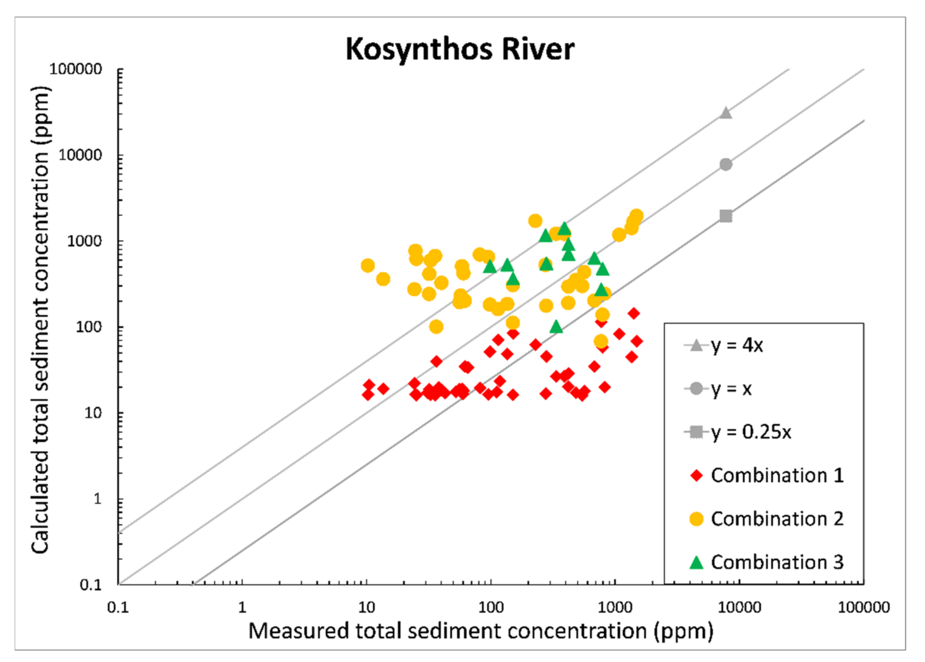
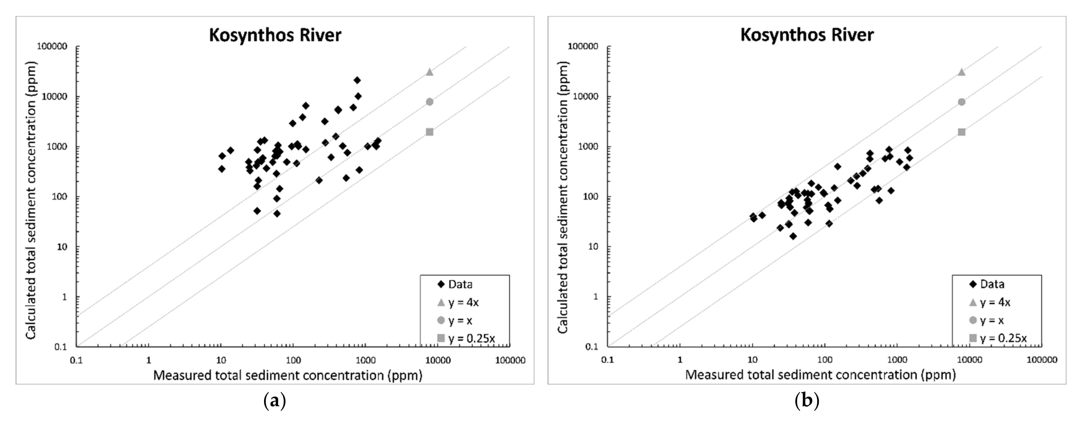
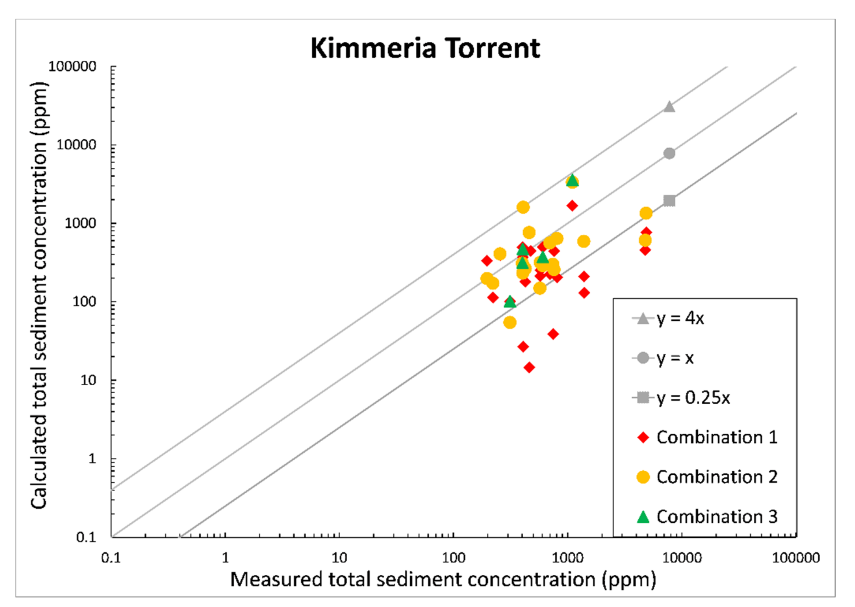
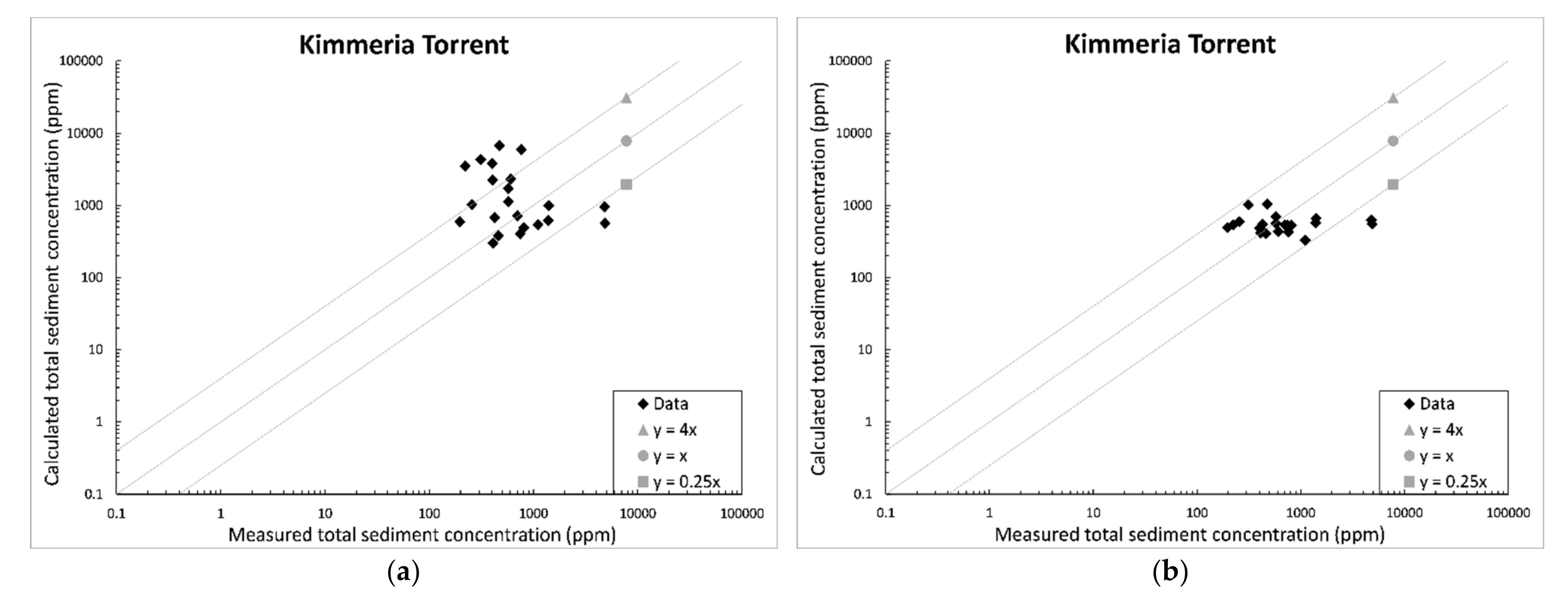
The results of the discrepancy ratio are illustrated in Figure 2, Figure 3, Figure 4, Figure 5, Figure 6 and Figure 7. Figure 2 and Figure 5 illustrate the discrepancy ratio between measured and calculated values of total sediment concentration by means of the combined equations. The plots of Figure 3a, Figure 4a, Figure 6a and Figure 7a represent the discrepancy ratio between measured and calculated values of total sediment concentration by means of the original formulas, whilst the plots of Figure 3b, Figure 4b, Figure 6b and Figure 7b represent the discrepancy ratio with the calibrated formulas. It should be noted that both coordinate axes in all plots are in logarithmic scale.
5. Discussion
In this paper, 84 sets of measurements were available: 62 field measurement data for Kosynthos River, for the period between 2005 and 2015, and 22 field measurement data for Kimmeria Torrent, for the period 2004–2015.
Table 5 illustrates that the first combination was applied to all sets of measured data, the second one used 41 sets and the third combination was implemented to 12 sets of measured data for Kosynthos River. For Kimmeria Torrent (Table 6), the first combination was carried out for all available data, the second combination was applied to 20 data sets and the third combination to five sets of measured data. The variation in the number of datasets that were used lies in the fact that no rainfall measurements were available for all the sediment transport measurements.
The discrepancy ratio plot between measured and calculated values of total sediment concentration by means of the combined equations and the fact that all the data sets were used prove that the first combination of the equations, in which suspended and bed load transport rates are expressed as a function of the stream discharge, has a better fit to the available data measurements of Kosynthos River. However, by examining the discrepancy ratio along with the R2 for the case study of Kimmeria Torrent, no safe conclusion could be established regarding the application of the combined equations to the available data. Overall, Figure 2 and Figure 5 show that all three combinations have better application in the case of Kosynthos River in comparison to Kimmeria Torrent. The reason for that is that more data sets were available for Kosynthos basin than Kimmeria basin.
Though the data for Kimmeria Torrent is limited, and the correlation is not satisfactory, the results are substantially improved by means of the calibrated Yang formulas. Given the intermittent and very low flow of Kimmeria Torrent, and the complex nature of the stream sediment transport processes, the estimation of total sediment load is a challenging task. The obtained results indicate the difficulty of modeling the total sediment load in intermittent streams and underline the need for further research. The main objective of the present study is to point out the need of calibrating/adjusting existing formulas to the specific conditions of the streams they are applied.
Regarding Yang’s formulas, their coefficients are redefined based on all available field measurements and the statistical criteria of both calibrated Yang’s formulas are improved in comparison to those of Yang’s original formulas. Specifically, the MRE displays a notable decrease, whilst the NSE, especially for Kosynthos River, is significantly improved. The linear correlation coefficient r and the determination coefficient R2 tend to the optimal values. Overall, the results can be considered satisfactory for the case of Kosynthos River, while for Kimmeria Torrent more data should be taken into account.
A similar project, regarding Nestos River [24], produced satisfactory results and proved that Yang’s formulas could be modified for a perennial river. In this study, 111 pairs of measured stream flow rate and measured total load transport rate in Nestos River were used and total sediment concentrations were calculated by means of Yang’s formulas, both original and calibrated. This enabled the comparison between calculated and site-measured total sediment concentrations. The statistical criteria of that study, shown in Table 7 and Table 8, indicate that the original Yang’s formulas do not describe the sediment transport rate of Nestos River as well as those of Kosynthos River. However, after the calibration of their coefficients using multiple linear regression, both Yang’s formulas were improved.
Although Nestos River differs from Kosynthos River in many parameters, such as water discharge, sediment transport rate and median particle diameter, Yang’s formulas can be successfully calibrated for both perennial and intermittent rivers.
This work demonstrates an efficient way for adjusting well-known sediment transport formulas, the global application of which could be questionable for the specific conditions of rivers and streams. It is, however, noted that the application of Equations (7) and (8) should be bounded in Kosynthos River and Equations (9) and (10) in Kimmeria Torrent.
6. Conclusions
There is a variety of equations and relationships that can be applied and developed in order to calculate the sediment transport rate, depending on the type of the stream and the available measurements.
In this study, three combinations of nonlinear regression equations were created based on the derived relationships between bed load transport rate and stream discharge, suspended load transport rate and rainfall depth, suspended load transport rate and rainfall intensity, and suspended load transport rate and stream discharge. On the basis of the above nonlinear regression equations, the total load transport rate was calculated indirectly as a function of stream discharge, rainfall depth and rainfall intensity. These relationships can be characterized as “hydrologic”. The comparison results between calculated and measured total load transport rates for Kosynthos River basin and Kimmeria Torrent basin (north-eastern Greece) are relatively satisfactory.
The suspended load transport rate was expressed mathematically as a function of rainfall characteristics and stream discharge, namely hydrologic variables, by means of regression equations, because the suspended material in a stream originates mainly from soil erosion products, due to rainfall and runoff, of the corresponding basin.
Total load transport rate was also calculated as a function of “hydraulic” variables, e.g., flow velocity, critical flow velocity, grain diameter, settling velocity, by means of Yang formulas for Kosynthos River and Kimmeria Torrent. Yang’s formulas constitute multiple nonlinear regression equations that were linearized in the present study.
The original 1973 Yang’s formula is based on the assumption of a critical situation, while, in the original 1979 Yang’s formula, a critical situation is not considered. The original 1973 Yang’s formula has a better fit to Kosynthos River than the original 1979 Yang’s formula. Regarding Kimmeria Torrent, the original 1979 Yang’s formula outperforms the original 1973 Yang’s formula, based on the available data. However, the “hydrologic” regression equations, especially the first combination, provide more satisfactory results than both original equations.
The arithmetic coefficients of the independent variables in the original Yang’s formulas were calibrated on the basis of the available “hydraulic” data for Kosynthos River and Kimmeria Torrent. Both calibrated Yang’s formulas provide more satisfactory results than the corresponding original formulas for both Kosynthos River and Kimmeria Torrent. The calibrated 1973 Yang’s formula outperforms the calibrated 1979 Yang’s formula for both Kosynthos River and Kimmeria Torrent.
Comparing the resulting modified equations for the intermittent Kosynthos River and Kimmeria Torrent and the perennial Nestos River, the more satisfactory values of the statistical criteria were achieved in the case study of Kosynthos River.
Both Yang’s formulas can be successfully calibrated for the intermittent watercourses of the present case studies, Kosynthos River and Kimmeria Torrent, provided that there are sufficient data available. This calls for further investigation, as the methods presented in this study could effectively remedy the lack of sediment data.
A natural follow-up of this study would be the application of regression analysis for determining the relationships between various, hydraulic and hydrologic, variables of ephemeral rivers, as well as the calibration of established sediment transport formulas. Along with the aforementioned study, Yang’s formulas could be applied and calibrated based on the available data measurements of ephemeral rivers.
Author Contributions
Conceptualization, V.H.; methodology, V.H. and K.K.; software, L.A. and K.K.; validation, L.A. and K.K.; formal analysis, L.A., K.K. and V.H.; investigation, K.K. and L.A.; resources, V.H. and K.K.; data curation, L.A.; writing—original draft preparation, L.A.; writing—review and editing, V.H., K.K. and L.A.; visualization, L.A.; supervision, V.H.; project administration, V.H. All authors have read and agreed to the published version of the manuscript.
Funding
This research received no external funding.
Institutional Review Board Statement
Not applicable.
Informed Consent Statement
Not applicable.
Data Availability Statement
Data are available upon request from the corresponding author.
Conflicts of Interest
The authors declare no conflict of interest.
References
- Kaffas, K.; Hrissanthou, V.; Sevastas, S. Modeling hydromorphological processes in a mountainous basin using a composite mathematical model and ArcSWAT. Catena 2018, 162, 108–129. [Google Scholar] [CrossRef]
- Mitra, B.; Scott, H.D.; Dixon, J.C.; McKimmey, J.M. Applications of fuzzy logic to the prediction of soil erosion in a large watershed. Geoderma 1998, 86, 183–209. [Google Scholar] [CrossRef]
- Kaffas, K.; Hrissanthou, V. Computation of hourly sediment discharges and annual sediment yields by means of two soil erosion models in a mountainous basin. Int. J. River Basin Manag. 2019, 17, 63–77. [Google Scholar] [CrossRef]
- Langbein, W.B.; Iseri, K.T. General Introduction and Hydrologic Definitions. In Manual of Hydrology: Part I. General Surface-Water Techniques; U.S. Government Printing Office: Washington, DC, USA, 1960; p. 28. [Google Scholar]
- Williamson, T.N.; Agouridis, C.T.; Barton, C.D.; Villines, J.A.; Lant, J.G. Classification of Ephemeral, Intermittent, and Perennial Stream Reaches Using a TOPMODEL-Based Approach. J. Am. Water Resour. Assoc. 2015, 51, 1739–1759. [Google Scholar] [CrossRef]
- Sefton, C.E.M.M.; Parry, S.; England, J.; Angell, G. Visualising and quantifying the variability of hydrological state in intermittent rivers. Fundam. Appl. Limnol. 2019, 193, 21–38. [Google Scholar] [CrossRef]
- Hinton, D.; Hotchkiss, R.; Ames, D.P. Comprehensive and Quality-Controlled Bedload Transport Database. J. Hydraul. Eng. 2017, 143, 06016024. [Google Scholar] [CrossRef]
- Kaffas, K.; Saridakis, M.; Spiliotis, M.; Hrissanthou, V.; Righetti, M. A fuzzy transformation of the classic stream sediment transport formula of Yang. Water 2020, 12, 257. [Google Scholar] [CrossRef] [Green Version]
- Meyer-Peter, E.; Müller, R. Formulas for bed load transport. In Proceedings of the IAHSR 2nd Meeting, Stockholm, Sweden, 7 June 1948; pp. 39–64. [Google Scholar]
- Einstein, H.A. The Bed-Load Function for Sediment Transportation in Open Channel Flows; U.S. Department of Agriculture: Washington, DC, USA, 1950.
- Yang, C.T. Incipient Motion and Sediment Transport. Proc. Asce Jnl. Hydr. Div. 1973, 99, 1679–1704. [Google Scholar] [CrossRef]
- van Rijn, L.C. Sediment Transport, Part I: Bed Load Transport. J. Hydraul. Eng. 1984, 110, 1431–1456. [Google Scholar] [CrossRef] [Green Version]
- Parker, G. Surface-based bedload transport relation for gravel rivers. J. Hydraul. Res. 1990, 28, 417–436. [Google Scholar] [CrossRef]
- Engelund, F.; Hansen, E. A Monograph on Sediment Transport in Alluvial Streams; Teknisk Forlag: Copenhagen, Denmark, 1967. [Google Scholar]
- Hinton, D.; Hotchkiss, R.H.; Cope, M. Comparison of Calibrated Empirical and Semi-Empirical Methods for Bedload Transport Rate Prediction in Gravel Bed Streams. J. Hydraul. Eng. 2018, 144, 04018038. [Google Scholar] [CrossRef]
- Wu, B.; van Maren, D.S.; Li, L. Predictability of sediment transport in the Yellow River using selected transport formulas. Int. J. Sediment Res. 2008, 23, 283–298. [Google Scholar] [CrossRef]
- Yang, C.T. Sediment Transport: Theory and Practice; McGraw-Hill: New York, NY, USA, 1996; ISBN 9780079122650. [Google Scholar]
- Yang, C.T. Unit stream power equations for total load. J. Hydrol. 1979, 40, 123–138. [Google Scholar] [CrossRef]
- Baniya, M.; Asaeda, T.; Shivaram, K.C.; Jayashanka, S. Hydraulic Parameters for Sediment Transport and Prediction of Suspended Sediment for Kali Gandaki River Basin, Himalaya, Nepal. Water 2019, 11, 1229. [Google Scholar] [CrossRef] [Green Version]
- Ulke, A.; Tayfur, G.; Ozkul, S. Predicting Suspended Sediment Loads and Missing Data for Gediz River, Turkey. J. Hydrol. Eng. 2009, 14, 954–965. [Google Scholar] [CrossRef] [Green Version]
- Angelis, I.; Metallinos, A.; Hrissanthou, V. Regression analysis between sediment transport rates and stream discharge for the Nestos River, Greece. Glob. Nest J. 2012, 14, 362–370. [Google Scholar]
- Kaffas, K.; Hrissanthou, V. Estimate of Continuous Sediment Graphs in a Basin, Using a Composite Mathematical Model. Environ. Process. 2015, 2, 361–378. [Google Scholar] [CrossRef] [Green Version]
- Metallinos, A.; Hrissanthou, V. Regression relationships between sediment yield and hydraulic and rainfall characteristics for two basins in northeastern Greece. In Proceedings of the Environmental Hydraulics—Proceedings of the 6th International Symposium on Environmental Hydraulics, Athens, Greece, 23–25 June 2010; Christodoulou, G., Stamou, A., Eds.; CRC Press/Balkema: Leiden, The Netherlands, 2010; Volume 2, pp. 899–904. [Google Scholar]
- Avgeris, L.; Kaffas, K.; Hrissanthou, V. Comparison between Calculation and Measurement of Total Sediment Load: Application to Nestos River. Environ. Sci. Proc. 2020, 2, 19. [Google Scholar] [CrossRef]
- Kitsikoudis, V.; Sidiropoulos, E.; Hrissanthou, V. Machine Learning Utilization for Bed Load Transport in Gravel-Bed Rivers. Water Resour Manag. 2014, 28, 3727–3743. [Google Scholar] [CrossRef]
- Laursen, E.M. The total sediment load of streams. J. Hydraul. Div. 1958, 84, 1–36. [Google Scholar] [CrossRef]
- Yang, C.T.; Marsooli, R.; Aalami, M.T. Evaluation of total load sediment transport formulas using ANN. Int. J. Sediment Res. 2009, 24, 274–286. [Google Scholar] [CrossRef]
- Hrissanthou, V. Simulation Model for the Computation of Sediment Yield due to Upland and Channel Erosion from a Large Basin. In Proceedings of the Porto Alegre Symposium; IAHS Publication: Wellington, UK, 1988; pp. 453–462. Available online: https://iahs.info/uploads/dms/iahs_174_0453.pdf (accessed on 3 December 2021).
- Hrissanthou, V.; Mylopoulos, N.; Tolikas, D.; Mylopoulos, Y. Simulation Modeling of Runoff, Groundwater Flow and Sediment Transport into Kastoria Lake, Greece. Water Resour. Manag. 2003, 17, 223–242. [Google Scholar] [CrossRef]
- Hrissanthou, V. Estimate of sediment yield in a basin without sediment data. Catena 2005, 64, 333–347. [Google Scholar] [CrossRef]
- Hrissanthou, V. Comparative application of two mathematical models to predict sedimentation in Yermasoyia Reservoir, Cyprus. Hydrol. Process. Int. J. 2006, 20, 3939–3952. [Google Scholar] [CrossRef]
- Andredaki, M.; Georgoulas, A.; Hrissanthou, V.; Kotsovinos, N. Assessment of reservoir sedimentation effect on coastal erosion in the case of Nestos River, Greece. Int. J. Sediment Res. 2014, 29, 34–48. [Google Scholar] [CrossRef] [Green Version]
- Gikas, G.D.; Yiannakopoulou, T.; Tsihrintzis, V.A. Modeling of non-point source pollution in a Mediterranean drainage basin. Environ. Model. Assess. 2006, 11, 219–233. [Google Scholar] [CrossRef]
- Krause, P.; Boyle, D.P.; Bäse, F. Comparison of different efficiency criteria for hydrological model assessment. Adv. Geosci. 2005, 5, 89–97. [Google Scholar] [CrossRef] [Green Version]
- Nash, J.E.; Sutcliffe, J.V. River flow forecasting through conceptual models part I—A discussion of principles. J. Hydrol. 1970, 10, 282–290. [Google Scholar] [CrossRef]
Figure 1.
Study area.

Figure 2.
Discrepancy ratio plot between measured and calculated values of total sediment concentration in Kosynthos River by means of the combined equations.
Figure 2.
Discrepancy ratio plot between measured and calculated values of total sediment concentration in Kosynthos River by means of the combined equations.

Figure 3.
Discrepancy ratio plot between measured and calculated values of total sediment concentration in Kosynthos River by means of the: (a) original Yang formula (1973) and (b) calibrated Yang formula (1973).
Figure 3.
Discrepancy ratio plot between measured and calculated values of total sediment concentration in Kosynthos River by means of the: (a) original Yang formula (1973) and (b) calibrated Yang formula (1973).

Figure 4.
Discrepancy ratio plot between measured and calculated values of total sediment concentration in Kosynthos River by means of the: (a) original Yang formula (1979) and (b) calibrated Yang formula (1979).
Figure 4.
Discrepancy ratio plot between measured and calculated values of total sediment concentration in Kosynthos River by means of the: (a) original Yang formula (1979) and (b) calibrated Yang formula (1979).

Figure 5.
Discrepancy ratio plot between measured and calculated values of total sediment concentration in Kimmeria Torrent by means of the combined equations.
Figure 5.
Discrepancy ratio plot between measured and calculated values of total sediment concentration in Kimmeria Torrent by means of the combined equations.

Figure 6.
Discrepancy ratio plot between measured and calculated values of total sediment concentration in Kimmeria Torrent by means of the: (a) original Yang formula (1973) and (b) calibrated Yang formula (1973).
Figure 6.
Discrepancy ratio plot between measured and calculated values of total sediment concentration in Kimmeria Torrent by means of the: (a) original Yang formula (1973) and (b) calibrated Yang formula (1973).

Figure 7.
Discrepancy ratio plot between measured and calculated values of total sediment concentration in Kimmeria Torrent by means of the: (a) original Yang formula (1979) and (b) calibrated Yang formula (1979).
Figure 7.
Discrepancy ratio plot between measured and calculated values of total sediment concentration in Kimmeria Torrent by means of the: (a) original Yang formula (1979) and (b) calibrated Yang formula (1979).


Table 1.
Hydrologic nonlinear regression relationships for Kosynthos River basin.
| Suspended Load Transport Rate versus Stream Discharge | Suspended Load Transport Rate versus Rainfall Depth | Suspended Load Transport Rate versus Rainfall Intensity | Bed Load Transport Rate versus Stream Discharge |
|---|---|---|---|
| y = 2.0491 exp (1.5402 x) | y = 0.1992 x2 − 19.806 x + 513.65 | y = −345.2 x2 + 1463.4 x + 36.294 | y = −0.0035 x5 + 0.0337 x4 − 0.1202 x3 + 0.1896 x2 − 0.1284 x + 0.0361 |
Table 2.
Hydrologic nonlinear regression relationships for Kimmeria Torrent basin.
| Suspended Load Transport Rate versus Stream Discharge | Suspended Load Transport Rate versus Rainfall Depth | Suspended Load Transport Rate versus Rainfall Intensity | Bed Load Transport Rate versus Stream Discharge |
|---|---|---|---|
| y = −702.2 x5 + 4542.9 x4 − 9727.5 x3 + 7997.2 x2 − 1995.5 x + 119.22 | y = −0.0029 x4 + 0.2278 x3 − 5.5178 x2 + 45.77 x + 20.374 | y = 0.0419 x3 − 3.1046 x2 + 64.056 x − 16.953 | y = −0.0273 x4 + 0.1494 x3 − 0.2596 x2 + 0.2018 x + 0.0079 |
Table 3.
Measured stream flow rate and total sediment concentration—calculated total sediment concentration in Kosynthos River.
Table 3.
Measured stream flow rate and total sediment concentration—calculated total sediment concentration in Kosynthos River.
| No | Stream Flow Rate (m3 s−1) | Total Load cF (Meas.) (ppm) | Total Load cF (Calc.) Original Yang 1973 (ppm) | Total Load cF (Calc.) Calibrated Yang 1973 (ppm) | Total Load cF (Calc.) Original Yang 1979 (ppm) | Total Load cF (Calc.) Calibrated Yang 1979 (ppm) | Combination 1 (ppm) | Combination 2 (ppm) | Combination 3 (ppm) |
|---|---|---|---|---|---|---|---|---|---|
| 1 | 0.43 | 335.8140 | 606.9675 | 291.9432 | 687.3276 | 319.9174 | 26.6573 | 1212.0674 | 101.9372 |
| 2 | 0.43 | 390.6977 | 1577.2966 | 366.1491 | 1792.6057 | 364.9354 | 26.6573 | 1212.0674 | 1416.9012 |
| 3 | 2.79 | 98.4946 | 2903.1226 | 113.6817 | 2701.8774 | 120.7814 | 51.6607 | 181.8078 | 511.0045 |
| 4 | 2.74 | 135.7664 | 3866.5061 | 148.8852 | 4008.2888 | 150.1945 | 48.7144 | 185.3100 | 528.6445 |
| 5 | 0.99 | 275.9596 | 3165.5488 | 255.5665 | 3468.8142 | 244.6086 | 16.8067 | 526.1865 | 1165.6607 |
| 6 | 3.20 | 150.9688 | 6520.0077 | 398.9830 | 6706.9759 | 372.4731 | 84.5233 | 112.0747 | 366.1508 |
| 7 | 2.68 | 280.0746 | 1177.9012 | 164.5355 | 960.8742 | 183.7974 | 45.4383 | 176.6227 | 549.8305 |
| 8 | 2.24 | 420.9375 | 5503.9324 | 568.6986 | 4801.4911 | 560.8989 | 28.7733 | 190.4951 | 706.3331 |
| 9 | 2.89 | 794.5329 | 10030.6309 | 632.1469 | 9075.8942 | 584.5008 | 58.1812 | 138.9315 | 475.7453 |
| 10 | 3.46 | 772.3121 | 21039.6846 | 872.2630 | 18227.9591 | 771.0490 | 115.5053 | 68.1192 | 272.8705 |
| 11 | 2.44 | 681.5574 | 5997.4014 | 571.9428 | 5190.2282 | 562.8918 | 34.8892 | 202.9815 | 634.8973 |
| 12 | 1.65 | 421.5152 | 5269.8290 | 727.9598 | 4484.3783 | 713.9938 | 20.2844 | 294.6348 | 920.3635 |
| 13 | 0.72 | 35.7064 | 1246.2457 | 124.1635 | 1443.8983 | 125.2208 | 16.1946 | 670.5773 | -- |
| 14 | 1.61 | 823.4988 | 340.1047 | 131.9498 | 503.6457 | 135.5321 | 20.0374 | 243.5369 | -- |
| 15 | 0.26 | 228.9318 | 213.4221 | 208.4815 | 419.7129 | 215.5683 | 62.2784 | 1708.4376 | -- |
| 16 | 0.68 | 95.4235 | 999.9242 | 120.0870 | 1152.2387 | 123.6992 | 16.4721 | 651.5061 | -- |
| 17 | 0.64 | 58.7231 | 668.6828 | 115.4120 | 766.5622 | 122.2408 | 16.9567 | 508.9825 | -- |
| 18 | 2.56 | 36.4975 | 509.6009 | 16.2327 | 755.3064 | 16.7229 | 39.7811 | 100.4242 | -- |
| 19 | 1.13 | 111.5372 | 460.2337 | 67.6208 | 598.9375 | 66.6613 | 17.5593 | -- | -- |
| 20 | 0.88 | 150.8719 | 869.0922 | 84.0420 | 949.9506 | 87.4506 | 16.2695 | 305.7240 | -- |
| 21 | 1.16 | 57.4119 | 808.8774 | 86.4070 | 889.4492 | 90.2433 | 17.7220 | 232.6690 | -- |
| 22 | 1.39 | 56.1637 | 643.7348 | 60.8842 | 776.0480 | 62.9939 | 18.8769 | 193.8200 | -- |
| 23 | 1.97 | 118.1591 | 1004.9264 | 56.7567 | 1120.4445 | 57.3948 | 23.5287 | -- | -- |
| 24 | 3.05 | 114.5769 | 1113.3538 | 28.8865 | 1412.1443 | 27.3677 | 70.8410 | 161.8150 | -- |
| 25 | 2.44 | 61.9491 | 1061.4399 | 52.0406 | 1254.2076 | 51.4907 | 34.8856 | 201.3962 | -- |
| 26 | 1.44 | 59.0078 | 285.8463 | 30.2175 | 594.0616 | 29.5393 | 19.1150 | -- | -- |
| 27 | 1.85 | 24.3287 | 495.7374 | 23.6265 | 712.3381 | 24.2399 | 22.0287 | 274.8598 | -- |
| 28 | 0.98 | 59.7626 | 91.3430 | 71.4738 | 467.5021 | 60.6577 | 16.7392 | -- | -- |
| 29 | 1.39 | 31.8719 | 159.4453 | 28.9519 | 563.8075 | 27.9248 | 18.8573 | 242.0712 | -- |
| 30 | 0.37 | 65.2952 | 790.4330 | 183.4181 | 1090.1627 | 172.6388 | 33.8823 | -- | -- |
| 31 | 0.90 | 10.2722 | 357.2231 | 40.2602 | 628.5402 | 42.0112 | 16.3661 | 518.1544 | -- |
| 32 | 0.54 | 81.8351 | 490.8300 | 154.0273 | 568.0208 | 160.1939 | 19.5752 | 694.3618 | -- |
| 33 | 1.07 | 485.6047 | 1019.9564 | 138.4587 | 881.7582 | 151.8081 | 17.2189 | 352.5406 | -- |
| 34 | 1.26 | 32.0713 | 850.4692 | 92.6831 | 807.8663 | 98.5171 | 18.2447 | 413.7905 | -- |
| 35 | 1.20 | 565.9081 | 749.2211 | 83.9788 | 747.1782 | 88.0473 | 17.9531 | 433.7064 | -- |
| 36 | 1.31 | 40.1614 | 1337.2851 | 126.8143 | 1425.4967 | 130.9070 | 18.4919 | 326.1858 | -- |
| 37 | 0.25 | 1490.9644 | 1310.4288 | 591.2591 | 1359.5938 | 587.7304 | 68.4937 | 1956.7439 | -- |
| 38 | 0.32 | 1359.4902 | 1081.9123 | 383.2361 | 1237.4700 | 374.9873 | 44.8738 | 1411.5200 | -- |
| 39 | 0.22 | 1080.8928 | 1007.7275 | 494.1553 | 1131.6184 | 491.9484 | 83.1688 | 1181.9161 | -- |
| 40 | 0.16 | 1411.7143 | 1004.9021 | 844.4405 | 1051.0541 | 866.7638 | 144.3981 | 1701.1444 | -- |
| 41 | 0.76 | 545.1180 | 234.9519 | 144.7907 | 477.6216 | 114.5575 | 16.0824 | 298.0294 | -- |
| 42 | 1.45 | 13.6481 | 830.0665 | 42.2166 | 849.9139 | 43.3873 | 19.1634 | 359.4885 | -- |
| 43 | 1.76 | 10.4712 | 647.9586 | 36.2533 | 732.0247 | 36.1116 | 21.1315 | -- | -- |
| 44 | 1.24 | 60.4020 | 653.8342 | 51.8893 | 738.7671 | 53.3864 | 18.1535 | 419.9050 | -- |
| 45 | 1.58 | 38.1351 | 590.9242 | 47.3734 | 703.7601 | 48.3790 | 19.8699 | -- | -- |
| 46 | 0.84 | 25.2489 | 329.4808 | 67.3573 | 540.2682 | 68.4105 | 16.1539 | 618.8063 | -- |
| 47 | 0.96 | 33.0981 | 209.6013 | 61.6282 | 484.6377 | 62.7791 | 16.6548 | -- | -- |
| 48 | 0.87 | 32.8566 | 491.6201 | 82.1484 | 606.0382 | 83.5098 | 16.2625 | 595.0111 | -- |
| 49 | 1.06 | 31.0041 | 416.1793 | 72.9338 | 573.9715 | 71.2795 | 17.1916 | -- | -- |
| 50 | 0.68 | 24.8344 | 387.1575 | 75.2133 | 559.6605 | 74.8298 | 16.4996 | 766.7018 | -- |
| 51 | 0.64 | 42.8419 | 365.9389 | 105.2314 | 526.9587 | 104.7744 | 17.0008 | -- | -- |
| 52 | 0.61 | 52.3821 | 483.4832 | 118.9038 | 622.3600 | 125.8161 | 17.5492 | -- | -- |
| 53 | 1.13 | 111.5372 | 460.2337 | 67.6208 | 598.9375 | 66.6613 | 17.5593 | -- | -- |
| 54 | 2.56 | 36.4975 | 509.6009 | 16.2327 | 755.3064 | 16.7229 | 39.7811 | -- | -- |
| 55 | 1.97 | 118.1591 | 1004.9264 | 56.7567 | 1120.4445 | 57.3948 | 23.5287 | -- | -- |
| 56 | 3.05 | 114.5769 | 1113.3538 | 28.8865 | 1412.1443 | 27.3677 | 70.8410 | -- | -- |
| 57 | 1.44 | 59.0078 | 285.8463 | 30.2175 | 594.0616 | 29.5393 | 19.1150 | -- | -- |
| 58 | 1.85 | 24.3287 | 495.7374 | 23.6265 | 712.3381 | 24.2399 | 22.0287 | -- | -- |
| 59 | 0.98 | 59.7626 | 45.7595 | 75.3405 | 461.7282 | 59.3784 | 16.7392 | -- | -- |
| 60 | 1.39 | 31.8719 | 52.0816 | 27.4987 | 520.7066 | 28.6008 | 18.8573 | -- | -- |
| 61 | 0.37 | 65.2952 | 143.6963 | 113.7347 | 416.0687 | 122.9017 | 33.8823 | -- | -- |
| 62 | 0.90 | 10.2722 | 357.2231 | 40.2602 | 628.5402 | 42.0112 | 16.3661 | -- | -- |
Table 4.
Measured stream flow rate and total sediment concentration—calculated total sediment concentration in Kimmeria Torrent.
Table 4.
Measured stream flow rate and total sediment concentration—calculated total sediment concentration in Kimmeria Torrent.
| No | Stream Flow Rate (m3 s−1) | Total Load cF (Meas.) (ppm) | Total Load cF (Calc.) Original Yang 1973 (ppm) | Total Load cF (Calc.) Calibrated Yang 1973 (ppm) | Total Load cF (Calc.) Original Yang 1979 (ppm) | Total Load cF (Calc.) Calibrated Yang 1979 (ppm) | Combination 1 (ppm) | Combination 2 (ppm) | Combination 3 (ppm) |
|---|---|---|---|---|---|---|---|---|---|
| 1 | 0.67 | 607.1642 | 2416.3347 | 425.7431 | 2332.9124 | 437.1424 | 497.2385 | 287.3469 | 373.0340 |
| 2 | 3.05 | 312.8525 | 3243.5092 | 1043.5132 | 4303.9802 | 1019.5731 | 100.8742 | 54.4245 | 101.2946 |
| 3 | 0.66 | 402.4242 | 3754.7200 | 492.4234 | 3780.0516 | 492.0866 | 498.4780 | 308.6660 | 314.5621 |
| 4 | 0.92 | 405.3804 | 2594.0813 | 450.9815 | 2257.3528 | 473.6653 | 369.3545 | 231.2532 | 471.6457 |
| 5 | 0.81 | 473.3827 | 5664.9279 | 1083.5447 | 6759.7054 | 1045.1551 | 444.0038 | -- | -- |
| 6 | 0.04 | 1102.5000 | 437.2637 | 302.4060 | 538.7160 | 331.3937 | 1678.7662 | 3326.5581 | 3573.8288 |
| 7 | 1.26 | 222.1270 | 3732.0542 | 521.4311 | 3515.1297 | 538.1428 | 113.3945 | 171.5556 | -- |
| 8 | 0.81 | 762.1235 | 7001.7301 | 421.6593 | 5931.9290 | 431.5201 | 444.0038 | 256.5022 | -- |
| 9 | 0.15 | 461.9125 | 241.4923 | 394.7844 | 383.2360 | 404.8596 | 14.5879 | 761.0303 | -- |
| 10 | 0.38 | 197.0604 | 580.8441 | 504.2258 | 595.0125 | 496.8450 | 332.5521 | 197.2796 | -- |
| 11 | 0.14 | 408.7243 | 73.5463 | 434.0411 | 299.9628 | 417.4983 | 26.6895 | 1597.8254 | -- |
| 12 | 0.30 | 809.3880 | 455.8342 | 557.4092 | 486.9880 | 530.7350 | 203.7949 | 637.7894 | -- |
| 13 | 0.20 | 745.6392 | 327.0242 | 584.0636 | 403.9684 | 535.9286 | 38.7167 | 298.9349 | -- |
| 14 | 0.43 | 256.3497 | 1569.7231 | 580.1319 | 1025.0548 | 594.1154 | 392.0229 | 406.7581 | -- |
| 15 | 1.16 | 426.9984 | 258.1951 | 443.0588 | 678.1001 | 547.6003 | 180.3820 | 263.4147 | -- |
| 16 | 0.30 | 1390.9597 | 334.9787 | 575.1409 | 616.0164 | 576.0628 | 210.1573 | 588.4338 | -- |
| 17 | 0.31 | 700.2786 | 545.3716 | 560.6055 | 719.2123 | 539.1392 | 224.6357 | 562.0170 | -- |
| 18 | 0.50 | 4801.3057 | 973.3962 | 693.2609 | 953.2653 | 629.2469 | 458.0387 | 607.0277 | -- |
| 19 | 1.89 | 574.0803 | 1949.6213 | 697.7435 | 1709.0208 | 697.7430 | 212.5039 | 148.6929 | -- |
| 20 | 0.06 | 4884.2681 | 310.5068 | 560.9651 | 565.1381 | 551.6226 | 765.8154 | 1339.4157 | -- |
| 21 | 1.07 | 576.9531 | 1299.8879 | 574.2564 | 1136.9432 | 567.0584 | 252.9423 | 316.5356 | -- |
| 22 | 1.23 | 1400.4858 | 1219.0957 | 708.2767 | 987.9857 | 660.2543 | 129.9650 | -- | -- |
Table 5.
Statistical criteria of combined equations, Yang’s original and calibrated formulas for Kosynthos River.
Table 5.
Statistical criteria of combined equations, Yang’s original and calibrated formulas for Kosynthos River.
| Number of Paired Values | MRE (%) | NSE | r | R2 | Discrepancy Ratio | |
|---|---|---|---|---|---|---|
| Original 1973 | 62 | −1226.540 | −83.404 | 0.317 | 0.101 | 0.226 |
| Calibrated 1973 | 62 | −37.293 | 0.521 | 0.766 | 0.587 | 0.968 |
| Original 1979 | 62 | −1577.191 | −66.701 | 0.306 | 0.094 | 0.177 |
| Calibrated 1979 | 62 | −38.302 | 0.522 | 0.776 | 0.602 | 0.887 |
| Combination 1 | 62 | 56.865 | −0.270 | 0.598 | 0.357 | 0.613 |
| Combination 2 | 41 | −598.067 | −0.349 | 0.543 | 0.295 | 0.561 |
| Combination 3 | 12 | −128.081 | −3.796 | −0.088 | 0.008 | 0.833 |
Table 6.
Statistical criteria of combined equations, Yang’s original and calibrated formulas for Kimmeria Torrent.
Table 6.
Statistical criteria of combined equations, Yang’s original and calibrated formulas for Kimmeria Torrent.
| Number of Paired Values | MRE (%) | NSE | r | R2 | Discrepancy Ratio | |
|---|---|---|---|---|---|---|
| Original 1973 | 22 | −298.247 | −3.248 | −0.244 | 0.059 | 0.500 |
| Calibrated 1973 | 22 | −14.884 | −0.114 | 0.069 | 0.005 | 0.909 |
| Original 1979 | 22 | −307.673 | −3.247 | −0.239 | 0.057 | 0.636 |
| Calibrated 1979 | 22 | −15.268 | −0.132 | 0.006 | 0.000 | 0.909 |
| Combination 1 | 22 | 43.135 | −0.180 | 0.298 | 0.089 | 0.682 |
| Combination 2 | 20 | 7.524 | −0.112 | 0.057 | 0.003 | 0.900 |
| Combination 3 | 5 | −22.497 | −14.312 | 0.954 | 0.910 | 1.000 |
Table 7.
Statistical criteria of Yang’s formulas (1973)—original and calibrated—for Nestos River.
| Number of Paired Values | MRE (%) | NSE | r | R2 | Discrepancy Ratio | |
|---|---|---|---|---|---|---|
| Original | 111 | −11,649.317 | −20.474 | 0.416 | 0.173 | 0.315 |
| Calibrated | 111 | −240.746 | 0.480 | 0.695 | 0.483 | 0.838 |
Table 8.
Statistical criteria of Yang’s formulas (1979)—original and calibrated—for Nestos River.
| Number of Paired Values | MRE (%) | NSE | r | R2 | Discrepancy Ratio | |
|---|---|---|---|---|---|---|
| Original | 111 | −16,196.804 | −35.110 | 0.491 | 0.241 | 0.243 |
| Calibrated | 111 | −218.745 | 0.492 | 0.716 | 0.513 | 0.820 |
Publisher’s Note: MDPI stays neutral with regard to jurisdictional claims in published maps and institutional affiliations. |
© 2022 by the authors. Licensee MDPI, Basel, Switzerland. This article is an open access article distributed under the terms and conditions of the Creative Commons Attribution (CC BY) license (https://creativecommons.org/licenses/by/4.0/).
Share and Cite
MDPI and ACS Style
Avgeris, L.; Kaffas, K.; Hrissanthou, V. Comparison between Calculation and Measurement of Total Sediment Load: Application to Streams of NE Greece. Geosciences 2022, 12, 91. https://0-doi-org.brum.beds.ac.uk/10.3390/geosciences12020091
AMA Style
Avgeris L, Kaffas K, Hrissanthou V. Comparison between Calculation and Measurement of Total Sediment Load: Application to Streams of NE Greece. Geosciences. 2022; 12(2):91. https://0-doi-org.brum.beds.ac.uk/10.3390/geosciences12020091
Chicago/Turabian StyleAvgeris, Loukas, Konstantinos Kaffas, and Vlassios Hrissanthou. 2022. "Comparison between Calculation and Measurement of Total Sediment Load: Application to Streams of NE Greece" Geosciences 12, no. 2: 91. https://0-doi-org.brum.beds.ac.uk/10.3390/geosciences12020091
Note that from the first issue of 2016, this journal uses article numbers instead of page numbers. See further details here.