
Numerical Modelling of Reactive Flows through Porous Media


Data61 CSIRO, Clayton 3168, Australia
Geosciences 2022, 12(4), 153; https://0-doi-org.brum.beds.ac.uk/10.3390/geosciences12040153
Submission received: 8 February 2022
/
Revised: 17 March 2022
/
Accepted: 22 March 2022
/
Published: 28 March 2022
(This article belongs to the Special Issue Digital Rock Analysis)
Abstract
:We consider a lattice Boltzmann (LB) model to solve the coupled Navier–Stokes and advection–diffusion equation with reactive boundary conditions at the interface between fluid and solid domains. The reactive boundary condition results in the position of the boundary changing continuously, and so boundary nodes may be partially filled with fluid at any instant. We develop the LB boundary conditions for both the velocity and concentration fields in the presence of partially filled boundary nodes and then validate this algorithm on some test cases—the Stefan problem for diffusion-dominated dissolution and kinetic-dominated dissolution. It is shown that the developed model agrees well with analytic results, so that they can be used for more general boundaries of arbitrary shape. Numerical simulations in three dimensions are then carried out on demonstration problems at various Peclet numbers to elucidate the transport mechanisms and their influence on solid grain dissolution.
Keywords:
lattice Boltzmann method; partially-filled voxel; Dirichlet boundary condition; diffusion; advectionPACS:
47.11.-j; 47.56.+r; 02.70.Ns1. Introduction
Reactive fluid flows occur in a variety of industrial, geochemical, and biological processes whereby chemical components in the fluid react with the solid matrix through which the fluid flows to either dissolve or precipitate on the solid. Some examples include leaching (to recover valuable minerals in a rock) [1], petroleum reservoir stimulation [2] and carbon sequestration [3], concrete and cement degradation due to dissolved chemicals [4], and bone tissue regeneration using porous scaffolds [5]. A feature of these processes is the temporal evolution of the solid matrix through which the fluid flows, which in turn affects how and where the fluid flows. Depending on what type of reaction and where the reaction occurs, fluid transport channels may either diminish or increase in dimensions. Fluid flow and solid matrix change are therefore intimately coupled, and important macroscopic quantities which engineers use to describe the ease of flow (such as permeability) evolve dynamically. Numerical modelling of such flows can yield insights into fundamental phenomena which are often opaque to experiments.
While there are a variety of numerical techniques which have been used to model such problems, e.g., direct numerical simulation via the finite volume method [3], recently, the lattice Boltzmann (LB) method has come to the fore [2,4]. The LB method can quantitatively model fluid transport for a wide variety of problems including advection, diffusion, and multi-component and multiphase fluid physics [6,7,8,9,10]. The method has become particularly widespread in modelling fluid transport through porous media, such as paper materials, fibres, porous rocks, etc., where the underlying solid matrix has a complicated topological structure. One of its main advantages comes from the fact that a digital image of the solid matrix (obtained from a computed tomography or CT scan or similar method) can be directly imported into an LB code to quantitatively predict fluid transport through the medium.
The digital image has a binary format where each voxel of the image may either be black (indicating a solid voxel) or white (indicating an empty or non-solid voxel). The LB method then solves the fluid dynamics equations on the empty voxels (or corresponding nodes in the LB method) with suitable boundary conditions applied at the interface between solid and non-solid voxels. When modelling fluid advection (sometimes also referred to as momentum transport), this boundary condition is most commonly the no-slip boundary condition, where the tangential component of the fluid’s velocity at the boundary is set to zero. One may also be interested in modelling transport via diffusion processes, whereby one solves a suitable advection–diffusion equation (with the field variable being either species concentration or temperature) with corresponding boundary conditions at the interface. This may be a Dirichlet boundary condition, which specifies the concentration at the boundary, or a Neumann condition, which contains information on the derivative of the concentration field. If this field is only transported by the velocity field (with no feedback, whereby the concentration field modifies the velocity), this field variable, C, satisfies
where is the velocity, t time, and D a diffusion parameter, which we assume here to be homogeneous through space, i.e., a constant. The classical LB treatment of boundaries considers the boundary to lie between an (empty) fluid node and a (full) solid node, depending on the LB relaxation time [11]. However, in reactive fluid flows, the solid boundary position changes in time (through growth or dissolution). The amount of solid volume change at a given voxel at each time step is not necessarily commensurate with the solid volume of a voxel. Thus, at any instant in time, some boundary (LB) nodes will contain both solid and fluid so that the boundary is no longer located midway between nodes. Previous works [2,4] specify particular criteria which converted a boundary voxel from solid to fluid (or vice versa) when the solid volume decreased below a threshold value. In this work, we attempt to develop an LB method which can encompass a gradual change in the interface voxel’s solid content.
While the LB method has (historically) operated on lattice nodes which are either fully fluid (or void) or fully solid, in recent years, there have been attempts to relax this constraint. One promising avenue of investigation is referred to as the partially saturated, or grayscale method [7,12,13,14,15,16]. In the grayscale model, lattice nodes can be partially fluid and are assigned a grayscale value between 0 (void) to 1 (solid). When solving for fluid flow, this results in an additional fluid drag on those lattice nodes with a non-zero grayscale value. The actual amount of drag is a function of that node’s grayscale value. Using this grayscale model, Pereira et al. [17,18,19] were able to determine permeabilities of real rock samples whose physical constitution could not be easily modelled with classical LB methods.
As mentioned above, in the context of reactive flows, certain boundary nodes which are initially fully solid may dissolve during the flow process (or conversely certain empty nodes may increase their solid content). Whilst the grayscale model has been developed so that one can solve the Navier–Stokes equations at these partially filled nodes, appropriate treatment of the boundary conditions for the advection–diffusion equation (Equation (1)) for partially filled boundary nodes needs to be derived and implemented. Equation (1) together with the Navier–Stoke equations for fluid flow are solved concurrently (and entirely) with the LB method. This is the focus of the present study.
2. Lattice Boltzmann Model
The central quantity in the Boltzmann transport equation, from which the LB method is derived, is the particle distribution function, , which denotes the distribution of particles at position , travelling with microscopic velocity at time t. In the LB method, this distribution function is discretised on a regular lattice so that particle positions are restricted to the lattice vertices (or nodes) with discrete velocity directions, . Generally, LB models can be classified as DmQn, where m denotes the number of dimensions of space and n the number of velocity directions. Common examples in one, two, and three dimensions are D1Q3, D2Q9, and D3Q19, and the discretised distribution function is denoted as where . The set of n vectors for each LB model are given in textbooks [7]. The time evolution of these distribution functions satisfy
where is a collision function involving particle pairs. In this work, we assume the simplified linear BGK [20] form
where is the equilibrium (Maxwell) distribution function [10] and the relaxation rate. Equation (2) contains both streaming of distribution functions, where distribution function is moved to the adjacent node at in one time-step and collision where distribution functions relax to their equilibrium value, according to a given relaxation rate. Equation (3) indicates that all distribution functions relax at the same rate to their equilibrium value. More complex multi-relaxation rate time schemes relax this constraint and have been shown to be more numerically robust and accurate [21], but for the purposes of this study, a single-relaxation model suffices.
The velocity field in Equation (1) is assumed here to be a solution of the Navier–Stokes equation, so the distribution function f satisfies:
where is the fluid density. A Chapman–Enskog expansion of Equation (2) indeed shows that the Navier–Stokes equations for continuity and momentum are recovered. Then, the macroscopic fluid viscosity in the Navier–Stokes equation is related to the relaxation rate in the LB collision process via , where is the sound speed given by and the macroscopic pressure is .
The concentration field can be transported by either diffusion or fluid advection. The fluid field (for advection of concentration field) is given by in Equation (1), which is determined above. To solve Equation (1), one defines a second set of distribution functions (analogous to f), . One follows the same prescription for the evolution of g as for f (i.e., Equation (2) but with a different relaxation parameter, ). A Chapman–Enskog expansion for g then shows that Equation (1) is recovered with the diffusivity D given by . The concentration field is given by
Boundary Conditions
We can now consider the boundary conditions which must be applied at fluid nodes which are adjacent to a solid node. For fluid flow, i.e., solving for f, one requires a no-slip boundary condition for the tangential component of the velocity. In the LB method this is achieved by applying the so-called bounce-back condition. After streaming, distribution functions which have been streamed onto the adjacent solid node are reversed in their direction. In the following time-step, these reversed distribution functions are then streamed back into the fluid. This has been shown to give a zero tangential velocity at a position halfway between the fluid and solid nodes [7,22] for a straight boundary. For the concentration field, we need to specify the concentration at the boundary. In this case, the g distribution functions that are entering the fluid lattice (after streaming) are unknown. Inamuro et al. [23] suggest to equate these distribution functions to their equilibrium values, i.e.,
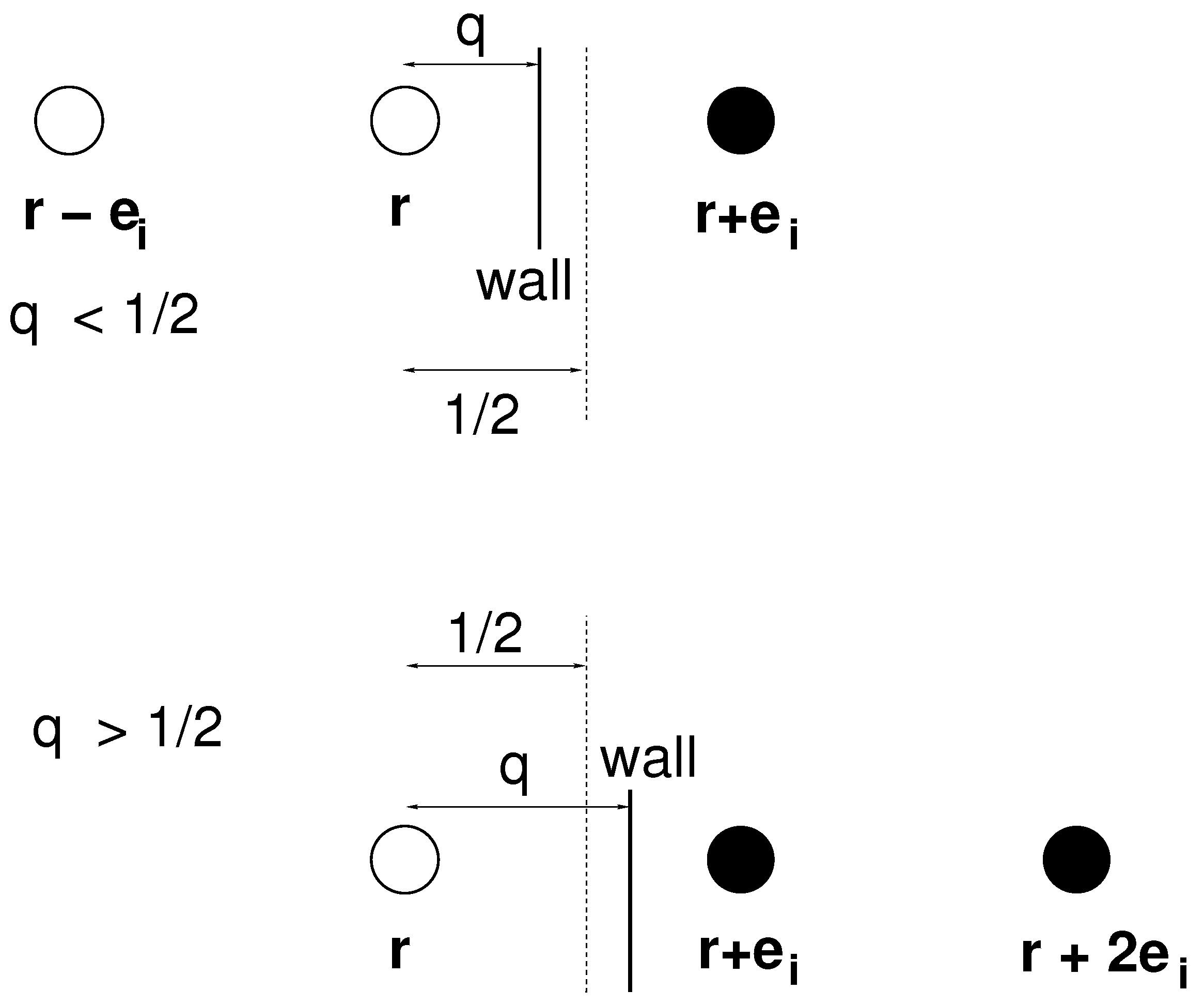
where is at the moment unknown and is the velocity of fluid in the (fluid) node adjacent to the wall (see Figure 1). The concentration at the boundary is specified, which we denote by . Then, since the sum of the s gives the concentration, when substituting Equation (6) into (5) at the boundary one obtains . We can solve this equation for and, consequently, the unknown incoming distribution functions. These two boundary conditions for f and g operate when the boundary is midway between a (full) solid node and an (empty) fluid node.
When the boundary changes position (due to, for example, reaction growth or dissolution), it is no longer located at the precise midway point between fluid and solid nodes and the above LB boundary implementations are not valid. Now the boundary nodes are, in fact, partially filled (with solid). For the fluid velocity field, we shall use a grayscale (sometimes also called partially saturated bounce-back) LB approach [7,12,13,14,15,16,17,18,19]. In this case, lattice nodes no longer need to be either full (solid) or empty (fluid) but can be some fraction filled, denoted by which is between 0 and 1. At these partially filled lattice nodes (which mark the boundary), we solve the following equation
The last term with the hat on the distribution function indicates that the distribution function to be added is in the opposite direction to i. The function can be simply (which is what we use in this work), although more complex forms such as
have been suggested by Noble and Torczynski [24]. Note that when , Equation (7) reduces to Equation (2), as required, and when , we have the bounce-back condition, as required. How the mineral (which is to be dissolved) is distributed through the solid grains will have an influence on the functional form of . At this stage, no assumptions can be made on this functionality, so a simple function form is implemented. However, in future this will be considered more closely by comparing different functional forms with actual experimental data.
The grayscale method only applies to the velocity field and so is unsuitable for the concentration field. Instead, we need to interpolate the g distribution functions at the partially filled boundary nodes [25,26,27]. These interpolated values can then be used in the Inamuro boundary condition [23]. To obtain interpolated g values, we consider Figure 1.
We define q as the distance of the last fluid node to the wall. For the case when , one obtains
Hats on distribution functions indicate they are coming into the fluid from outside the fluid domain. The first term on the right-hand side of Equation (9) is an incoming distribution function into a fluid node and so is unknown. All other distribution functions in these equations are known (in addition, those distribution functions that do not traverse the boundary are known). For the unknown distribution functions, we once again assume they take their equilibrium values (Inamuro boundary condition) with an (as yet) unknown concentration . The difference to the previous case is that this term now contains the multiplicative prefactor . We can once again determine the unknown by using Equation (5) and the specified value of the boundary concentration, .
For the second term on the right-hand side of Equation (11) and first term on right-hand side of Equation (12), we need to extrapolate the boundary values [7,27]. Using linear extrapolation, and , and substituting these back into Equations (11) and (12), one ends up with the same expressions as in Equations (9) and (10). Then, we use the same procedure as for to obtain the unknown distribution functions.
3. Comparison between LB and Analytical Results
We now apply the results derived above to two important scenarios where the boundary position changes with time. The two cases have known analytic solutions so that the new LB boundary condition can be validated. These are a Stefan problem, for diffusion-dominated flow [26,28], and a kinetic reactive boundary condition, where kinetics dominate variation in the boundary position [26].
In the first case of the Stefan problem, we consider a planar interface between the fluid and solid regions, so that the problem is effectively one-dimensional. The Stefan problem is solved in the region and the solid region extends from . We solve Equation (1) with initial condition (for ) and boundary conditions , (at all times) and at , when reaction kinetics is instantaneous compared to diffusion, as shown by Verhaeghe et al. (see Section II of [26]), we obtain
Note that . is the difference in the species concentration between the solid and liquid at the interface. This solid region diminishes in time (due to dissolution specified in Equation (13)) and so the boundary at is the position-variable boundary. Initially, the interface is midway between solid and liquid nodes. As solid content diminishes in the solid node, the position of interface is updated according to Equation (13) and, consequently, q (distance of liquid node to wall) is also updated. Then, using Equations (5) and (9), we can update solid concentration (and associated) values in any interface nodes. This process is iterated at each LB time-step.
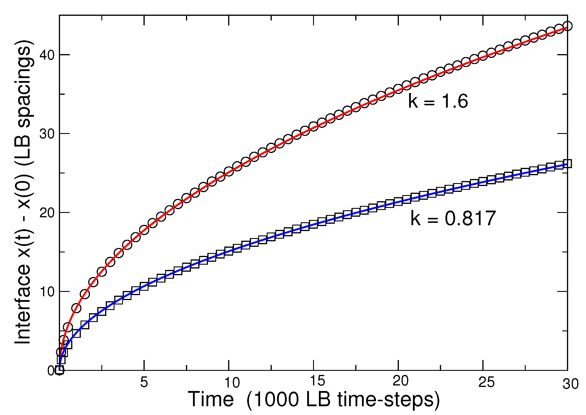
Aaron et al. [28] give the analytic solution for the problem that depends on a parameter k which is given by . The interface at is given by , where is a complicated function of k [28]. We use the LB boundary condition derived above to model this boundary problem. The actual numerical solution is calculated with a D3Q19 model with periodic boundary conditions in the y and z directions. We set the initial (solid–liquid) boundary at and the length of the lattice is . In Figure 2 we compare the LB solution with the analytic solution for two k values. Very good agreement is found in both cases.
In the second case of the kinetic boundary conditions, we use a similar setup to that of the Stefan problem, but with boundary condition (13) replaced by
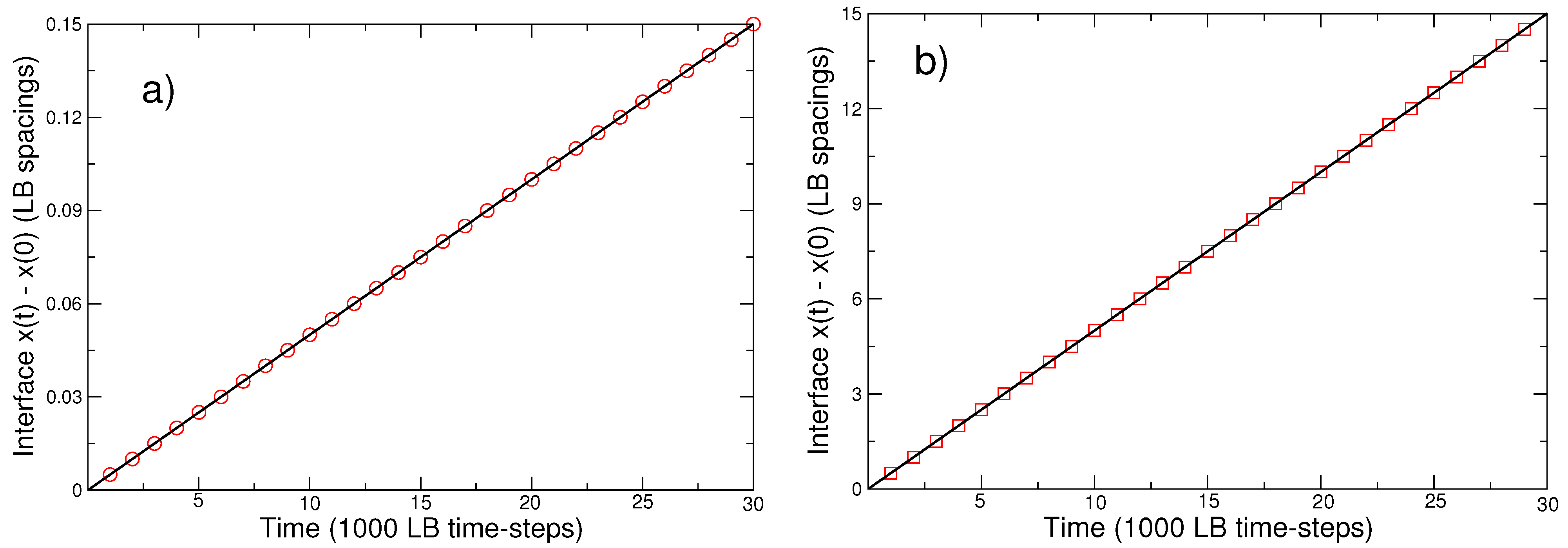
where is the kinetic reaction rate. The analytic solution of this problem [26] is . The LB setup is similar to the Stefan problem, except for the boundary condition at (Equation (14)). The solution for two different values is given in Figure 3a,b. Again, very good agreement is found.
We also considered diffusion and kinetic boundary conditions for a solid cylinder surrounded by liquid. In the case of kinetic boundary conditions, the interface between solid and fluid regions changes linearly with time [26,29], which was verified in our simulation. More interestingly, the dissolution of a solid, square disc evolves differently based on the particular boundary condition (diffusion of kinetic) that is implemented. For a diffusive boundary condition, the corners of the square gradually smoothen, so that the square shape dissolves to a circle whose radius slowly decreases with time. On the other hand, for kinetic boundary conditions, during dissolution, the square retains that shape, but its edge length decreases gradually. This behaviour is in agreement with previous studies [26].
4. Three-Dimensional Flow, Diffusion, and Reaction
Next, we consider more practical applications of the model to a three-dimensional (3D) solid geometry with non-negligible fluid flow, which couples the Navier–Stokes and advection–diffusion equations in a non-trivial manner. Although not a true porous medium, we consider a collection of a few cubical solid grains (with sharp corners) and consider the passage of a fluid through this domain. Fluid flow is introduced through the inclusion of a pressure gradient which is attained by setting the particle densities appropriately at the inlet and outlet [19]. Recall that in the LB method, the particle density, , and pressure, P, are related via , where is the sound speed. In this artificial problem, we assume solvent is initially only present at the inlet and then either is advected or diffuses through the fluid domain. Reactions between the solvent and mineral (in the solid grain) result in dissolution of the solid grain, and the precipitate is carried away in solution.
The boundary condition at the interface between fluid and the solid grain, where a reaction may occur, is a linear kinetic (rate) boundary condition. At the boundary sites where mineral dissolution occurs, we implement a substrate source–sink term in Equation (7), as outlined by Patel et al. [4]. This substrate source–sink term, , is added to the right-hand side of the advection–diffusion equation (Equation (1)),
only at those fluid sites which are adjacent to a solid site at which a reaction may take place. Since the LB solution of the advection–diffusion equation is treated similarly to the Navier–Stokes equation, with the substitution of the distribution functions for the distributions, it is straightforward to see that the presence of in the advection–diffusion equation is equivalent to a body force in the Navier–Stokes equation. Hence, we may use a similar solution procedure for Equation (15) as we do for the Navier–Stokes equation with a body force [19,30].
To ensure that the LB implementation of this boundary source–sink term in Equation (15) is correct, one can carry out a standard validation problem [2,4] in which one solves the diffusion equation in a rectangular domain. Linear reactive boundary conditions are placed on one edge, and on an adjacent edge, a constant concentration, while the remaining boundaries are no-flux. This problem has an analytical solution given in standard texts [31]. We implemented this test problem and reproduced the analytical results. However, since this test has stationary boundaries, it is not influenced by our newly developed boundary conditions from Section 2. Thus, we do not reproduce the results here.
Non-Trivial Pore-Scale Geometry
The solid–fluid domain through which fluid flows is shown in Figure 4. Fluid flows in the positive z-direction with the inlet/outlet at the bottom/top of the domain. Periodic boundary conditions are used in the x and y directions. Since the flow velocity is non-negligible, there are two distinct regimes which are important to consider. To understand this, it is convenient to define the non-dimensional Peclet number, Pe, of the flow. The Peclet number is defined as the ratio of advective transport to diffusive transport and is given by Pe . Here, is a characteristic fluid velocity, W a typical inter-channel separation, and D the diffusion constant. If the flow velocity is significant and/or the diffusion constant small (i.e., advection dominant), the corresponding Peclet number is large, while if the flow velocity is small and/or the diffusion constant large (i.e., diffusion dominant), the Peclet number is small.
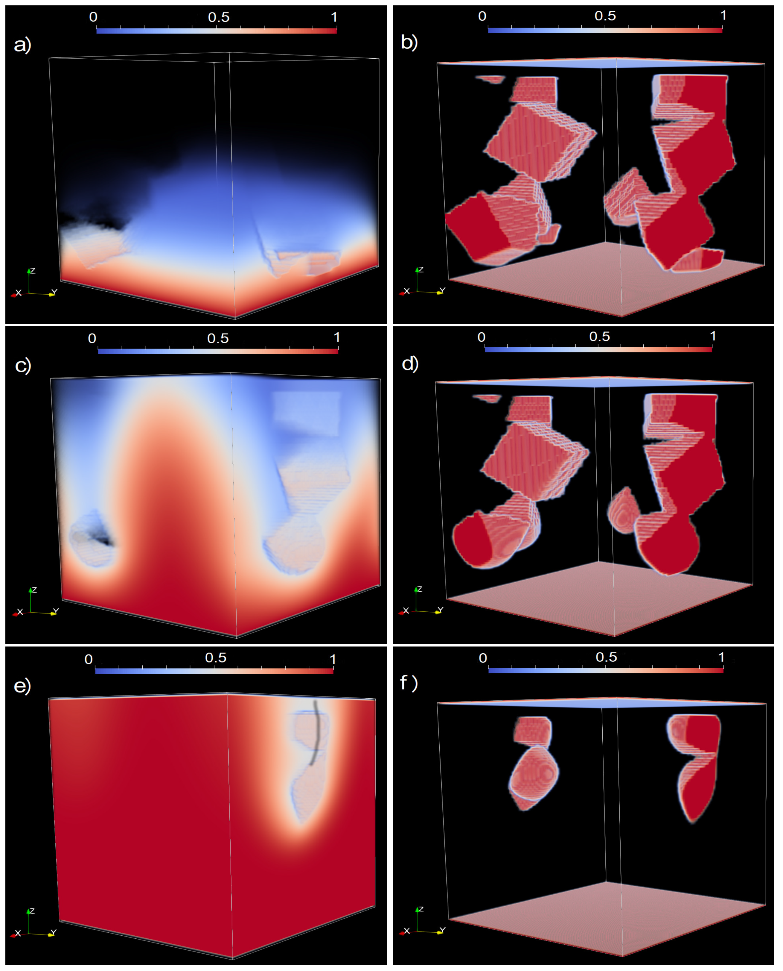
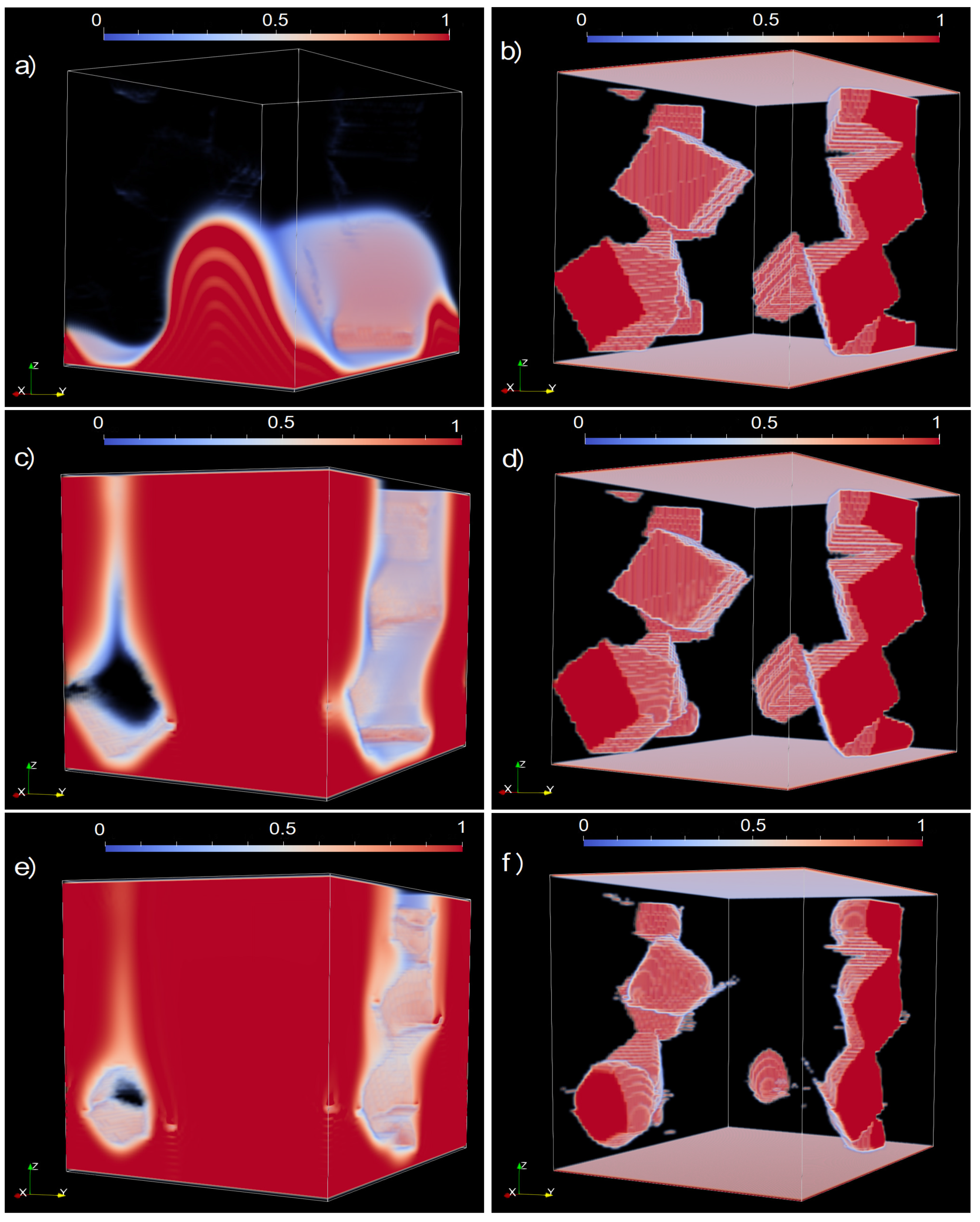
In the first case, we use an LB diffusion relaxation rate of which gives a diffusion constant, D, of 1.666 while the pressure gradient used is . Once the flow has stabilised, we determine that the Peclet number for this flow was 0.1, which makes it a diffusion-dominated flow. Figure 5 shows the solvent concentration (left column) and mineral content (right column) at three different times during the flow. Early on (top two snapshots), the solvent is only present in significant concentration at the bottom of the domain and, correspondingly, the solid grain structure remains largely unaffected. As time proceeds (middle snapshots), the solvent concentration advances roughly as a uniform front, except for solid regions which inhibit progress of the front. This is indicative of diffusive behaviour. One observes, at the corresponding time, that the mineral content of the bottom section of the domain dissolves away more-or-less as a flat front. This is clear if one looks at the solid cubes in the top half of the domain. At this stage, they all possess their original sharp corners, which indicates the diffusion front has not reached the higher zones in the domain. The final time (bottom two snapshots) reinforces this behaviour with the solid region below where the solvent front has reached (roughly half to one-third of the way up the domain), being dissolved away while solid grains in the top zone are still visible. It is clear that the large diffusion constant results in diffusion being the major transport mechanism for the solvent. As we shall see below, the actual time taken for solid grains to dissolve is considerably smaller than for an advection-dominant flow.
In the second case, we use an LB diffusion relaxation rate of which gives a diffusion constant, D, of 3.33 , while the pressure gradient is the same as before, at . In this case, we estimate that the Peclet number of the flow is approximately 1000, and so the main solvent transport mechanism is via fluid advection. Fluid will typically flow through the widest channels and tend to bypass narrow channels. This can be seen in the snapshots at the first time-step shown in Figure 6. The solvent front is observed to pass through the wide channel in the middle of the domain. At the same time, the solid grain structure has changed very little from the beginning, which indicates that the solvent has not come sufficiently close to the solid grains for a reaction to be initiated. At the next set of snapshots, the solvent concentration has formed a continuous pathway from the bottom of the domain (inlet) to the top (outlet). However, at the same time, the solid grains show minor changes from the previous snapshot. The main difference is that some of the cubes’ corners appear a little more rounded. The final snapshot, at the end of the simulation, shows that solvent concentration has not reached the grains well away from the main (central) flow path. As such, the solid grains remain largely intact and most noticeably (in contrast to the diffusion case) still exist throughout the domain (from bottom to top).
For this (large Peclet number) flow, fluid primarily flows through the large central channel from inlet to outlet. There is insignificant lateral flow (in x and y directions). Only solid grains that are adjacent to the central fluid flow channel come in contact with solvent, and they dissolve only slightly. Since the diffusion constant is very small, solvent is not transported to any significant extent away from the central channel, and the solid grain structure remains almost entirely intact.
The actual time taken for solid grains to dissolve in a diffusion-dominant flow is considerably smaller than for an advection-dominant flow. For the diffusion-dominant flow, it took around 126,000 LB time-steps for the domain to be cleared, while for the advection-dominant case, even by LB time-steps (last snapshot in Figure 6), the solid grains were visible and their initial structure could still be discerned. Diffusion is a better transport mechanism for the solvent as it allows the solvent to reach all lateral extents of the domain. However, fluid advection is much less efficient at reaching all the lateral regions of the domain, since fluid will preferentially bypass the smallest channels and flow through the main channel (in the middle of the domain). Since the diffusion constant is so small in the second case, it takes an extremely long time for solvent to be transported through the smallest channels and hence those solid grains which are distant from the main channel remain intact for a long time.
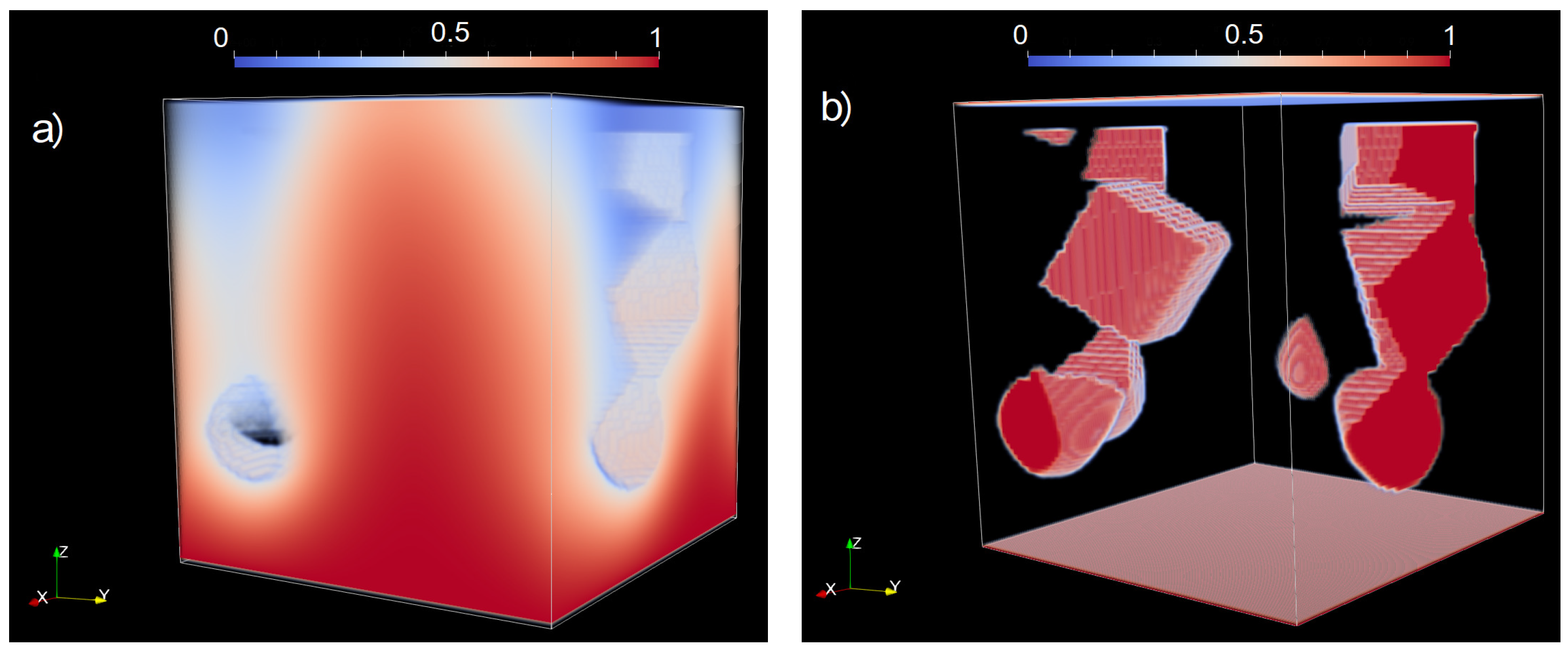
A more realistic Peclet number (indicative of real fluids and flow conditions) lies somewhere between these two extreme cases. However, the extreme cases have clearly shown us the roles of the different fluid transport mechanisms. In a third case, we used an LB diffusion relaxation rate of , which gives a diffusion constant of 3.33 , while the pressure gradient remains the same at . The corresponding Peclet number is then approximately 10. Rather than showing a number of snapshots, we just show the solvent concentration and mineral content midway through the flood (Figure 7). The solvent concentration has formed a continuous pathway from inlet to outlet through the central fluid channel, but has also spread across the bottom quarter of the domain. At the corresponding time, solid grains have dissolved away not only at the bottom of the domain (due to diffusion) but also at the top right, due to a combination of advection and diffusion from the central fluid channel. For this Peclet number, the time taken to dissolve all the solid grains was 176,000 LB time-steps, which is larger than the diffusion-dominated case.
5. Conclusions
In this study, we have considered a coupled fluid flow–concentration–reaction problem where lattice nodes at the fluid–solid boundary may be partially filled. For the velocity field, a grayscale boundary condition is applied, while for the concentration field, the Dirichlet boundary condition is obtained through a combination of interpolation and extrapolation. These new boundary conditions were validated on benchmark problems for diffusive (Stefan problem) and kinetic boundary conditions (linear rate) and showed excellent agreement with analytic solutions for a planar liquid–solid interface. These boundary conditions were also applied to more general shapes (circular and square) and were able to produce sensible results. Reactions in this model are accommodated through an additional source–sink term in the advection–diffusion equation.
We then implemented this coupled fluid flow, diffusion, and reaction model on some more general (demonstration) scenarios, to investigate the physical behaviour of the model. We were able to consider a range of advection and diffusion regimes and understand how dissolution may be affected. For large Peclet number (advection-dominant), the dissolution process is slow, since the solvent is mainly transported through the large fluid channels. Thus, any solid grains remote from this fluid channel will be bypassed, since the diffusion constant is small, will rarely be reached by the solvent. On the other hand, for small Peclet number (diffusion-dominant), the solvent advances as a uniform front (independently of the fluid velocity) and hence the dissolution is much more uniform and rapid. While the model has been implemented on simple, demonstration problems, in the future we intend to couple it with realistic chemistry, but this study has exhibited the capacity of the developed model to capture realistic physical behaviour.
Funding
This research received no external funding.
Institutional Review Board Statement
Not applicable.
Informed Consent Statement
Not applicable.
Data Availability Statement
Not applicable.
Conflicts of Interest
The authors declare no conflict of interest.
References
- Cross, M.; Bennett, C.R.; Croft, T.N.; Mcbride, D.; Gebhardt, H. Computational modeling of reactive multi-phase flows in porous media: Applications to metals extraction and environmental recovery processes. Min. Eng. 2006, 19, 1098–1108. [Google Scholar] [CrossRef]
- Chen, L.; Kang, Q.J.; Robinson, B.A.; He, Y.-L.; Tao, W.-Q. Pore-scale modelling of multiphase reactive transport with phase transitions and dissolution-precipitation processes in closed systems. Phys. Rev. E 2013, 87, 043306. [Google Scholar] [CrossRef] [Green Version]
- Molins, S.; Trebotich, D.; Steefel, C.I.; Shen, C.-P. An investigation of the effect of pore scale flow on average geochemical reaction rates using direct numerical simulation. Water Resour. Res. 2012, 48, W03527. [Google Scholar]
- Patel, R.A.; Phung, Q.T.; Seetharam, S.C.; Perko, J.; Jacques, D.; Maes, N.; De Schutter, G.; Ye, G.; Van Breugel, K. Diffusivity of saturated ordinary Portland cement-based materials: A critical review of experimental and analytical modelling approaches. Cem. Concr. Res. 2016, 90, 52–72. [Google Scholar] [CrossRef]
- Voronov, R.; VanGordon, S.; Sikavitsas, V.I.; Papavassiliou, D.V. Computational modelling of flow-induced shear stresses with 3D salt-leached poeour scaffolds imaged via micro-CT. J. Biomech. 2010, 43, 1279–1286. [Google Scholar] [CrossRef] [PubMed]
- Succi, S. The Lattice Boltzmann Equation for Fluid Dynamics and Beyond; Clarendon Press: Oxford, UK, 2001. [Google Scholar]
- Kruger, T.; Kusumaatmaja, H.; Kuzmin, A.; Shardt, O.; Silva, G.; Viggen, E. The Lattice Boltzmann Method. Principles and Practice, 1st ed.; Springer: Cham, Switzerland, 2017. [Google Scholar]
- Aidun, C.K.; Clausen, J.R. Lattice-Boltzmann method for complex flows. Ann. Rev. Fluid Mech. 2010, 42, 439–472. [Google Scholar] [CrossRef]
- Chen, S.; Doolen, G.D. Lattice Boltzmann method for fluid flows. Ann. Rev. Fluid Mech. 1996, 30, 329–364. [Google Scholar] [CrossRef] [Green Version]
- Liu, H.-H.; Kang, Q.-J.; Leornardi, C.R.; Schmiechek, S.; Narvez, A.; Jones, B.D.; Williams, J.R.; Valocchi, A.J.; Harting, J. Multiphase lattice-Boltzmann simulations for porous media applications. Computat. Geosci. 2016, 20, 777–805. [Google Scholar] [CrossRef] [Green Version]
- Talon, L.; Bauer, D.; Gland, N.; Youseff, S.; Auradou, H.; Ginzburg, I. Assessment of the two relaxation Lattice Boltzmann scheme to simulate Stokes flow in porous media. Water Resour. Res. 2012, 48, W04526. [Google Scholar] [CrossRef]
- Balasubramaniam, K.; Hayot, F.; Saam, W.F. Darcy’s law from lattice-gas hydrodynamics. Phys. Rev. A 1987, 36, 2248–2253. [Google Scholar] [CrossRef]
- Gao, Y.; Sharma, M.M. A LGA model for fluid-flow in heterogeneous porous media. Transp. Porous Media 1994, 17, 1–17. [Google Scholar] [CrossRef]
- Dardis, O.; McCloskey, J. Lattice Boltzmann scheme with real numbered solid density for the simulation of flow in porous media. Phys. Rev. E 1998, 57, 4834–4837. [Google Scholar] [CrossRef]
- Thorne, D.T.; Sukop, M.C. Lattice Boltzmann approach to Richard’s equation. Dev. Water Sci. 2004, 55, 1549. [Google Scholar]
- Zhu, J.J.; Ma, S. An improved gray lattice Boltzmann model for simulating fluid flow in multi-scale porous media. Adv. Water Resourc. 2013, 56, 61–76. [Google Scholar] [CrossRef]
- Li, R.R.; Yang, S.; Pan, J.-X.; Pereira, G.G.; Taylor, J.A.; Clennell, B.; Zou, C. Lattice Boltzmann modelling of permeability of porous materials with partially percolating voxels. Phys. Rev. E 2014, 90, 033301. [Google Scholar] [CrossRef] [PubMed]
- Pereira, G.G.; Wu, B.; Ahmed, A. Lattice Boltzmann heat transfer model for permeable voxels. Phys. Rev. E 2017, 96, 063108. [Google Scholar] [CrossRef]
- Pereira, G.G. Fluid flow, relative permeabilities and capillary pressure curves through heterogeneous porous media. Appl. Math. Model. 2019, 75, 481–493. [Google Scholar] [CrossRef]
- Bhatnager, P.I.; Gross, E.P.; Krook, M. A model for collision processes in gases. 1. Small amplitude processes in charged and neutral one-component systems. Phys. Rev. 1954, 94, 511–525. [Google Scholar] [CrossRef]
- D’Humieres, D.; Ginzburg, I.; Krafczyk, M.; Lallem, P.; Luo, L.-S. Multiple-relaxation-time lattice Boltzmann models in three dimensions. Philos. Trans. R. Soc. Lond. Ser. Math. Phys. Eng. Sci. 2002, 360, 437–451. [Google Scholar] [CrossRef]
- Ginzbourg, I.; Adler, P.M. Boundary flow condition analysis for the three-dimensional lattice Boltzmann model. J. Phys. II Fr. 1994, 4, 191–214. [Google Scholar] [CrossRef]
- Inamuro, T.; Yoshino, T.M.; Inoue, H.; Mizuno, R.; Ogino, F. A lattice Boltzmann method for a binary miscible fluid mixture and its application to a heat-transfer problem. J. Comput. Phys. 2002, 179, 201–215. [Google Scholar] [CrossRef] [Green Version]
- Noble, D.R.; Torczynski, J.R. A lattice Boltzmann method for partially saturated computational cells. Int. J. Mod. Phys. 1998, 9, 1189–1201. [Google Scholar] [CrossRef]
- Bouzidi, M.; Firdaouss, P. Lallemand, Momentum transfer of a Boltzmann-lattice fluid with boundaries. Phys. Fluids 2001, 13, 3452–3459. [Google Scholar] [CrossRef]
- Verhaeghe, F.; Arnout, S.; Blanpain, B.; Wollants, P. Lattice-Boltzmann modelling of dissolution phenomena. Phys. Rev. 2006, 73, 036316. [Google Scholar]
- Walsh, S.D.C.; Saar, M.O. Interpolated lattice Boltzmann boundary conditions for surface reaction kinetics. Phys. Rev. 2010, 82, 066703. [Google Scholar] [CrossRef] [Green Version]
- Aaron, H.B.; Fainstein, D.; Kotler, G.R. Diffusion limited phase transformations: A comparison and critical evaluation of the mathematical approximations. J. Appl. Phys. 1970, 41, 4404–4410. [Google Scholar] [CrossRef]
- Habashi, F. Principles of Extractive Metallurgy; Gordon and Breach: New York, NY, USA, 1969. [Google Scholar]
- Seta, T. Implicit temperature-correction-based immersed-boundary thermal lattice Boltzmann method for the simulation of natural convection. Phys. Rev. 2013, 87, 063304. [Google Scholar] [CrossRef] [Green Version]
- Carslaw, H.S.; Jaeger, J.C. Conduction of Heat in Solids; Oxford University Press: New York, NY, USA, 1986. [Google Scholar]
Figure 1.
Diagram for calculating Dirichlet boundary conditions for concentration field when boundary nodes are partially filled. White circles denote fluid nodes and black circles are solid nodes. The node at is the last node before the wall (vertical black line) and may be partially filled with fluid.

Figure 2.
Results of solution of Stefan problem from LB (symbols) and analytic results (lines) with diffusion constant and k shown next to each set of results.
Figure 2.
Results of solution of Stefan problem from LB (symbols) and analytic results (lines) with diffusion constant and k shown next to each set of results.

Figure 3.
Comparison of numerical LB results (symbols) versus analytic result (lines) for the rapid kinetic reaction. In (a) the reaction rate is , and in (b) , while for both.
Figure 3.
Comparison of numerical LB results (symbols) versus analytic result (lines) for the rapid kinetic reaction. In (a) the reaction rate is , and in (b) , while for both.

Figure 4.
Three-dimensional geometrical domain composed of solid, cubical grains (blue) and fluid region (void). Fluid inlet is at the bottom of the domain while outlet is at the top with a pressure gradient in positive z direction. Periodic boundary conditions are in other (x and y) directions.
Figure 4.
Three-dimensional geometrical domain composed of solid, cubical grains (blue) and fluid region (void). Fluid inlet is at the bottom of the domain while outlet is at the top with a pressure gradient in positive z direction. Periodic boundary conditions are in other (x and y) directions.

Figure 5.
Solvent and mineral distributions at various stages during a small Peclet number (Pe = 0.1) flow. (a) Solvent concentration at initial stages, (b) mineral content at initial stages, (c) solvent concentration at middle stages, (d) mineral content at middle stages, (e) solvent concentration at final stage, and (f) mineral content at final stage.

Figure 6.
Solvent and mineral distributions at various stages during a large Peclet number (Pe = 1000) flow. (a) Solvent concentration at initial stages, (b) mineral content at initial stages, (c) solvent concentration at middle stages, (d) mineral content at middle stages, (e) solvent concentration at final stage, and (f) mineral content at final stage.

Figure 7.
Solvent and mineral distributions during an intermediate Peclet number (Pe = 10) flow. (a) Solvent concentration and (b) mineral content.
Figure 7.
Solvent and mineral distributions during an intermediate Peclet number (Pe = 10) flow. (a) Solvent concentration and (b) mineral content.

Publisher’s Note: MDPI stays neutral with regard to jurisdictional claims in published maps and institutional affiliations. |
© 2022 by the author. Licensee MDPI, Basel, Switzerland. This article is an open access article distributed under the terms and conditions of the Creative Commons Attribution (CC BY) license (https://creativecommons.org/licenses/by/4.0/).
Share and Cite
MDPI and ACS Style
Pereira, G.G. Numerical Modelling of Reactive Flows through Porous Media. Geosciences 2022, 12, 153. https://0-doi-org.brum.beds.ac.uk/10.3390/geosciences12040153
AMA Style
Pereira GG. Numerical Modelling of Reactive Flows through Porous Media. Geosciences. 2022; 12(4):153. https://0-doi-org.brum.beds.ac.uk/10.3390/geosciences12040153
Chicago/Turabian StylePereira, Gerald G. 2022. "Numerical Modelling of Reactive Flows through Porous Media" Geosciences 12, no. 4: 153. https://0-doi-org.brum.beds.ac.uk/10.3390/geosciences12040153
Note that from the first issue of 2016, this journal uses article numbers instead of page numbers. See further details here.