
Shallow Landslides and Rockfalls Velocity Assessment at Regional Scale: A Methodology Based on a Morphometric Approach

 , , and
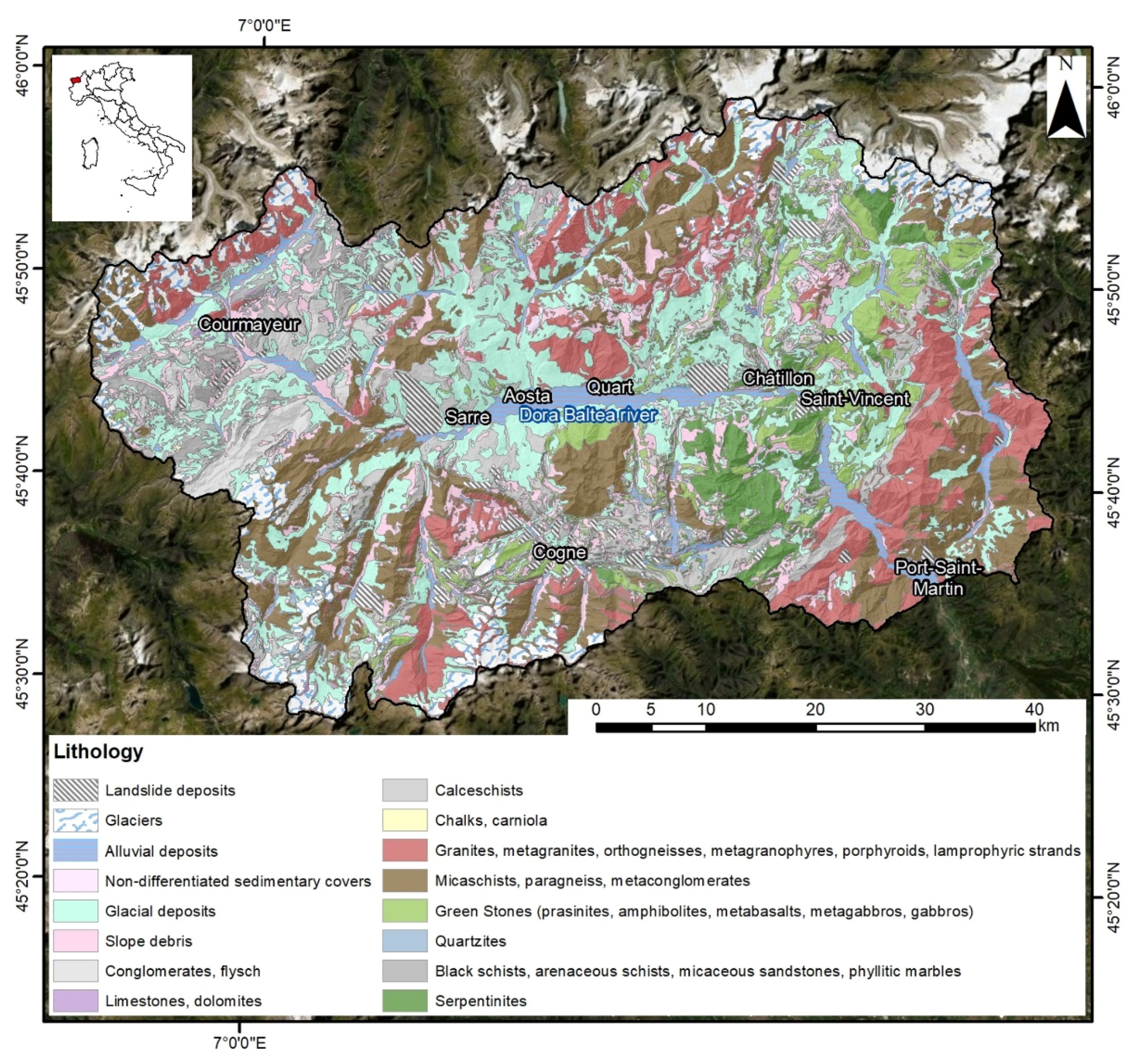
Abstract
:1. Introduction
2. Materials and Methods
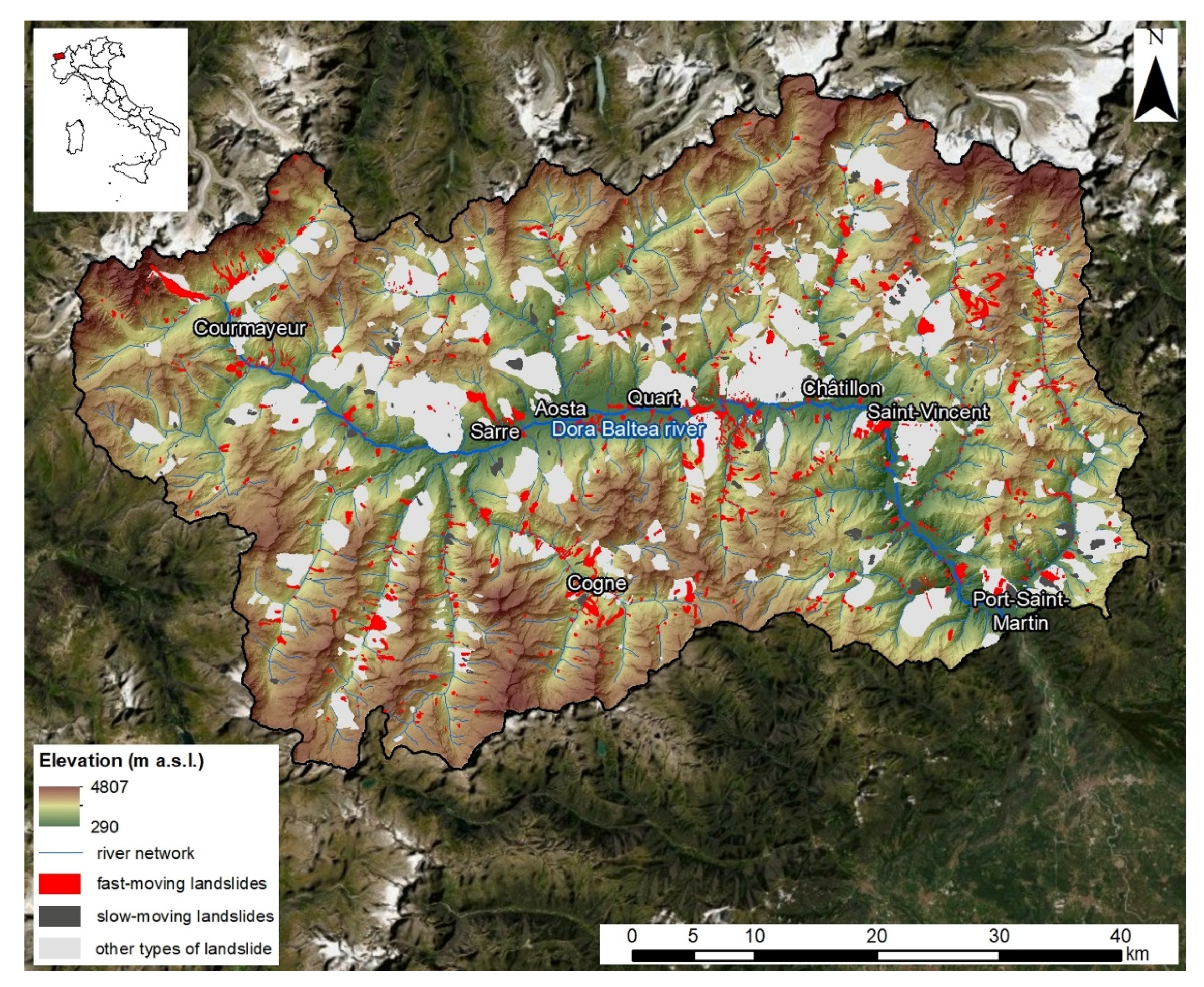
2.1. Study Area
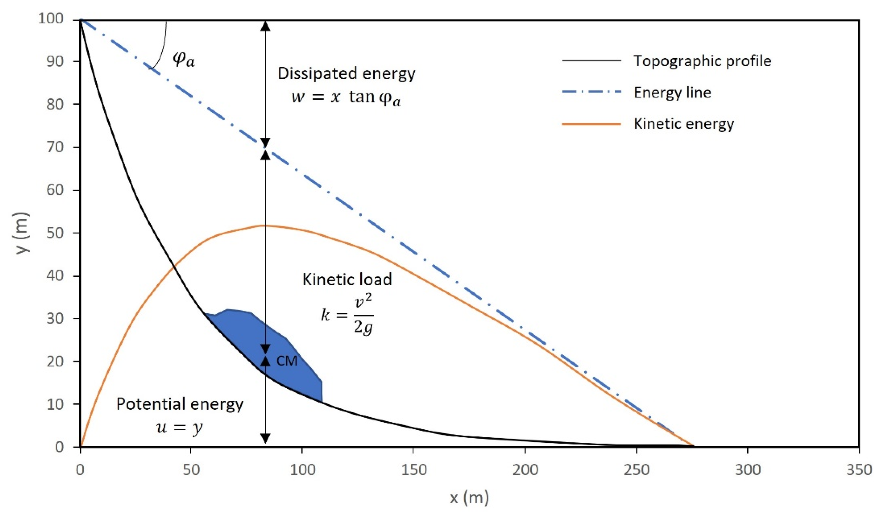
2.2. Heim Method
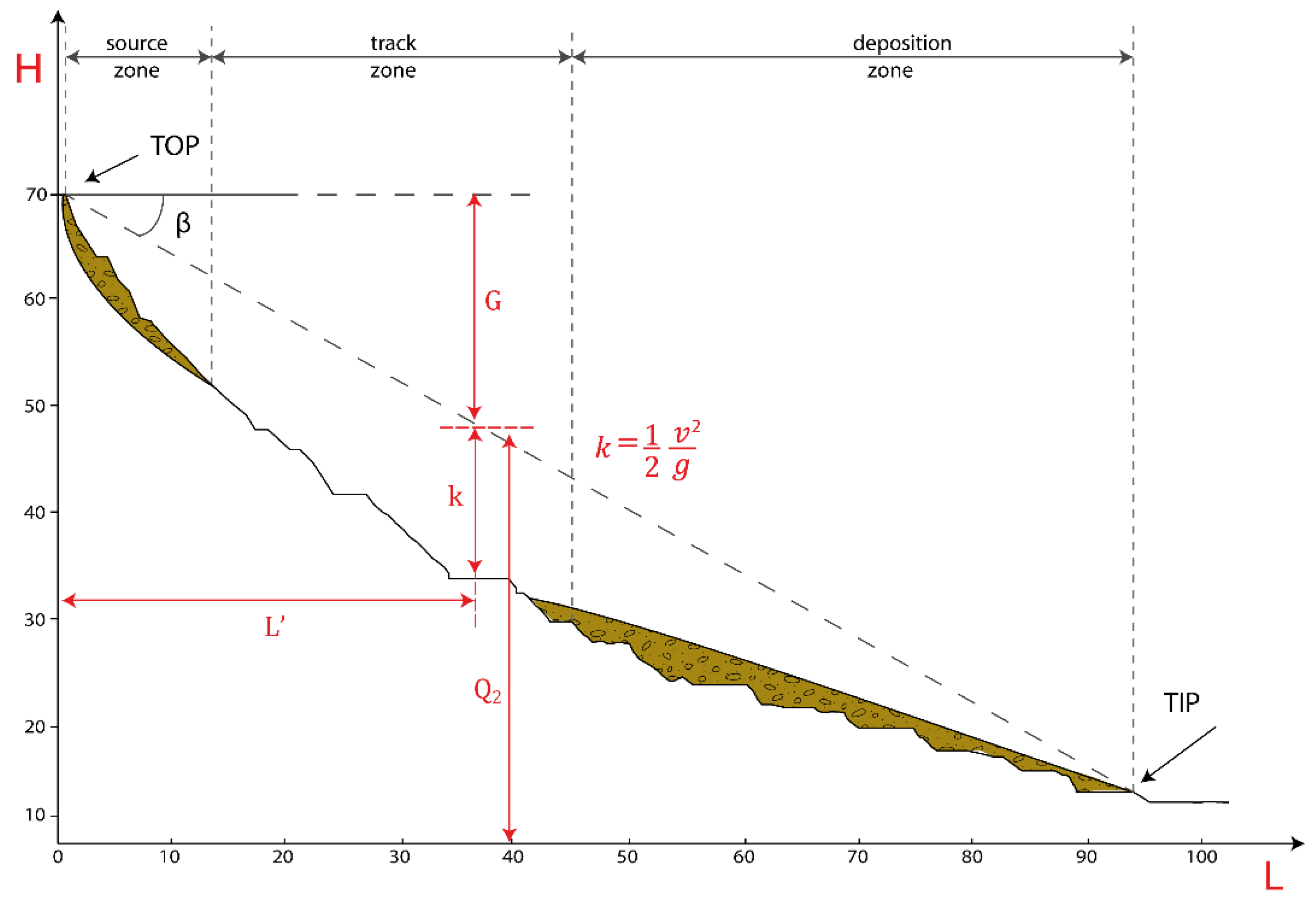
2.3. Input Data Preparation and Elaboration
- (1)
- L’—horizontal distance of each point within the landslide from the top;
- (2)
- Tanβ—tangent of the propagation angle (constant for each landslide);
- (3)
- G—vertical distance between the top and the energy line, G = L’ × tanβ;
- (4)
- Q2—height of the energy line, Q2 = Qmax–G;
- (5)
- k—kinetic load, k = Q2—landslide point elevation (DEM).
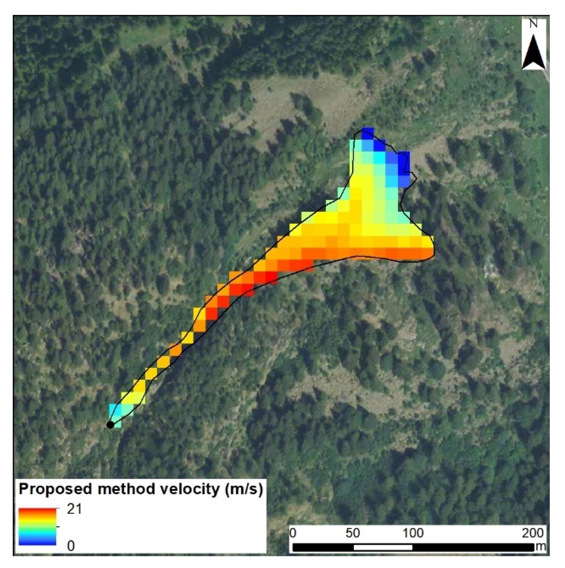
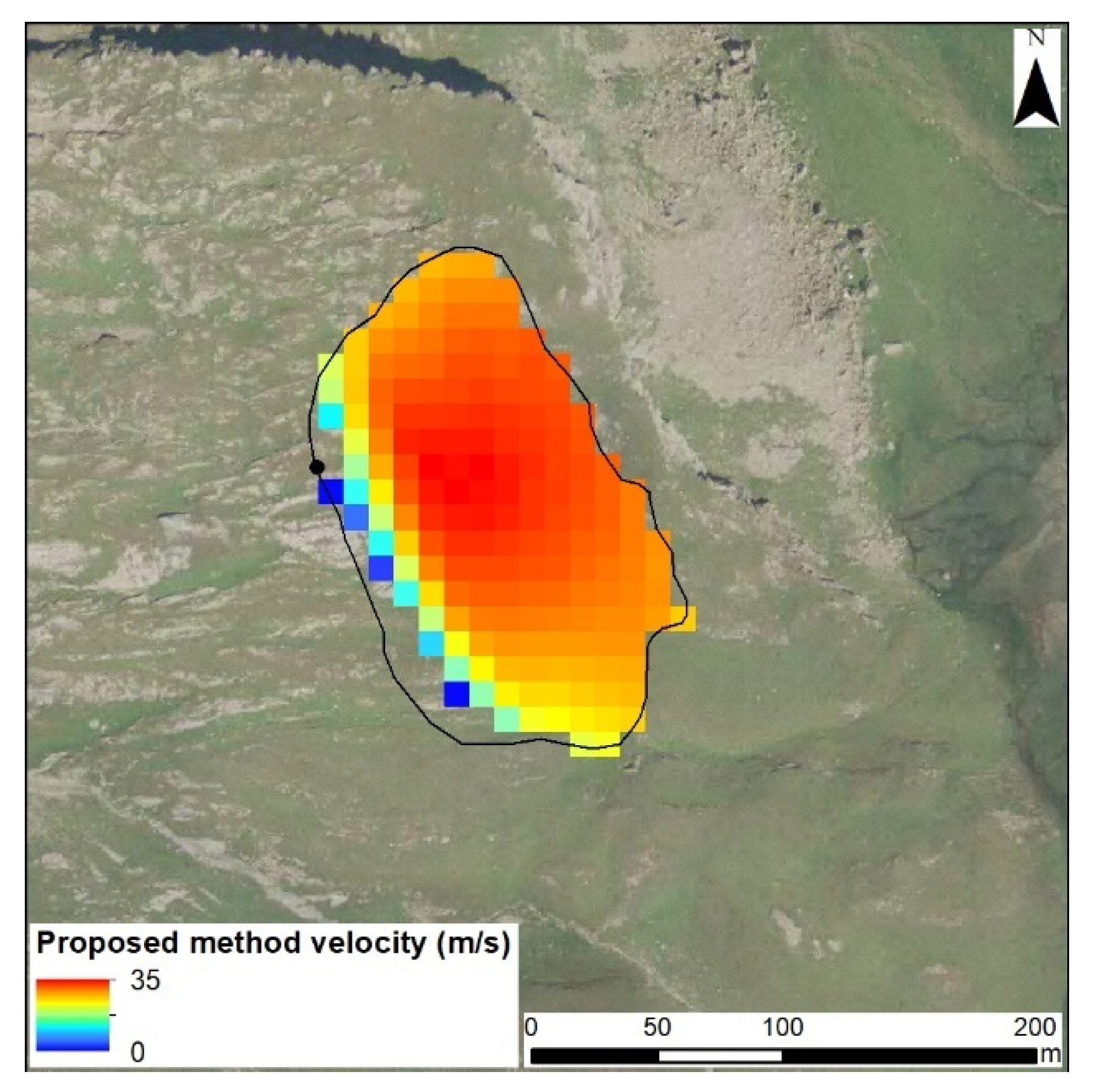
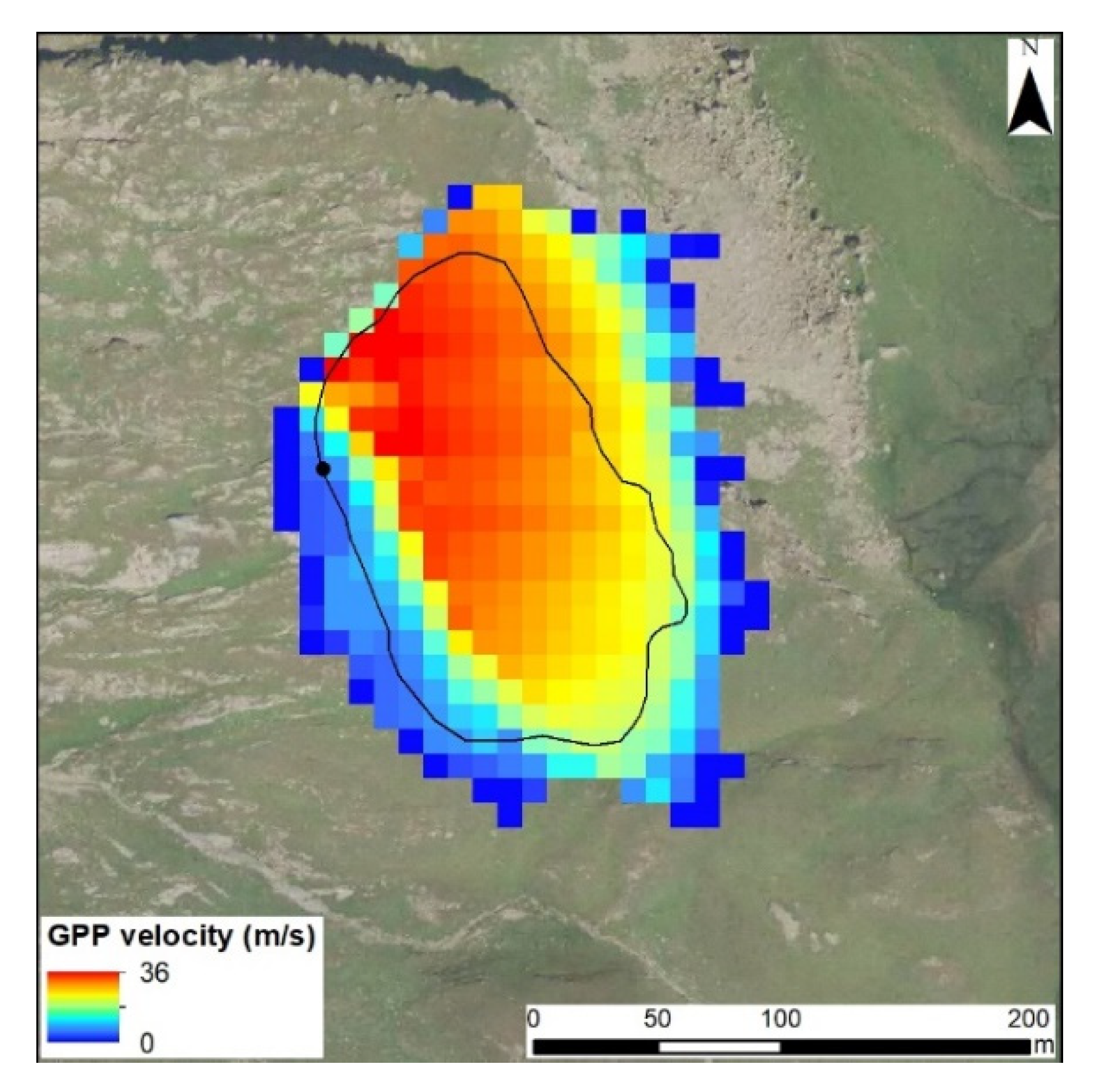
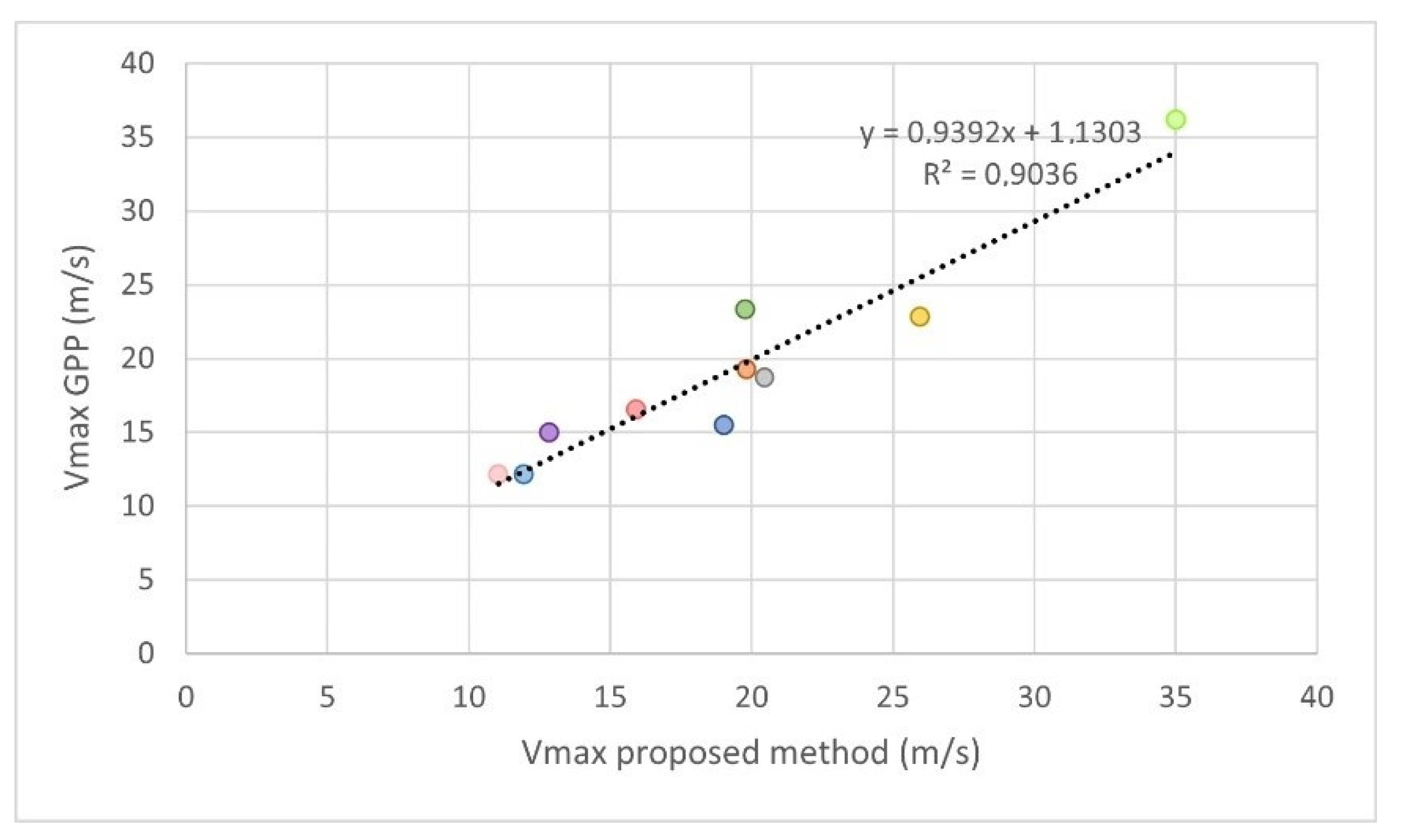
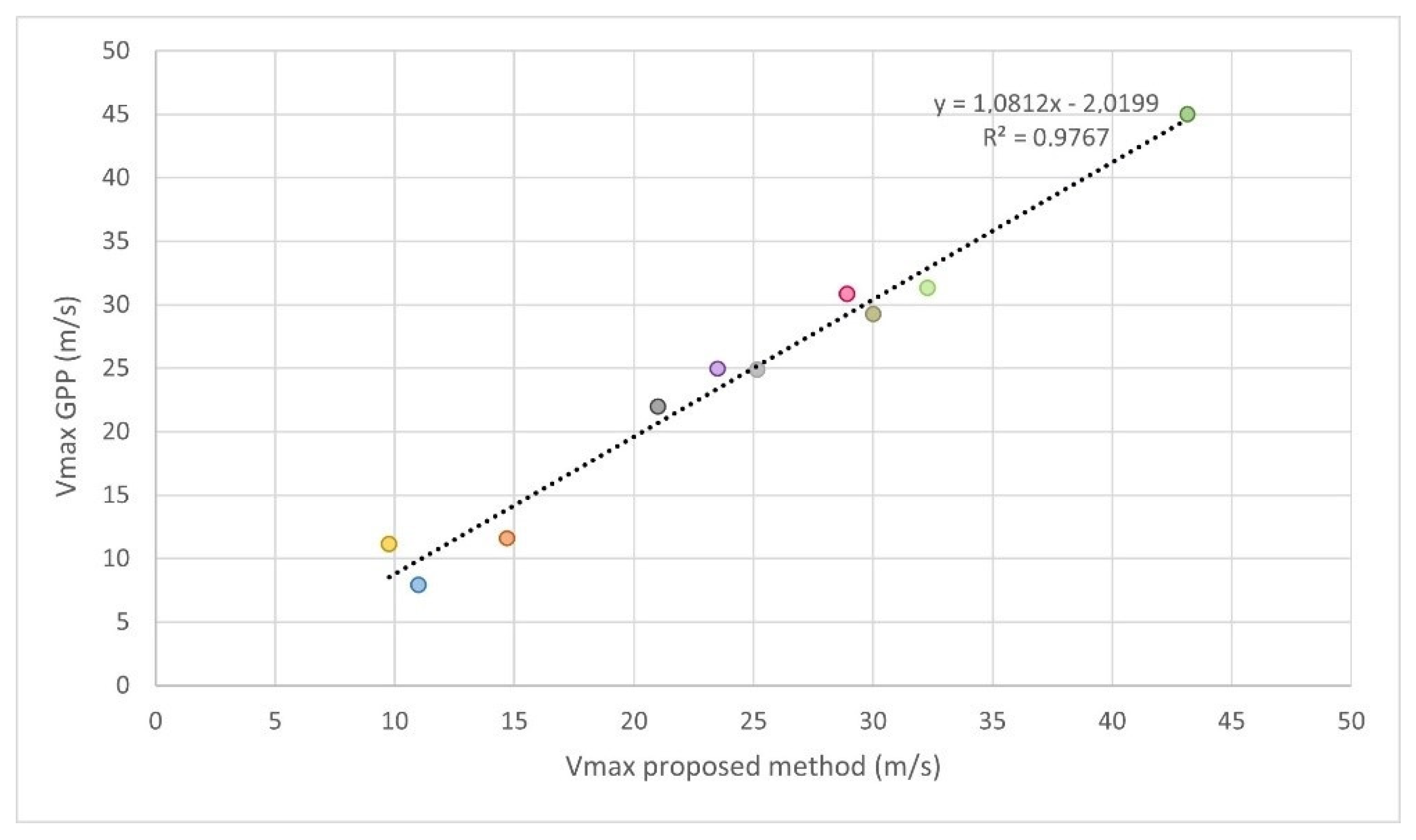
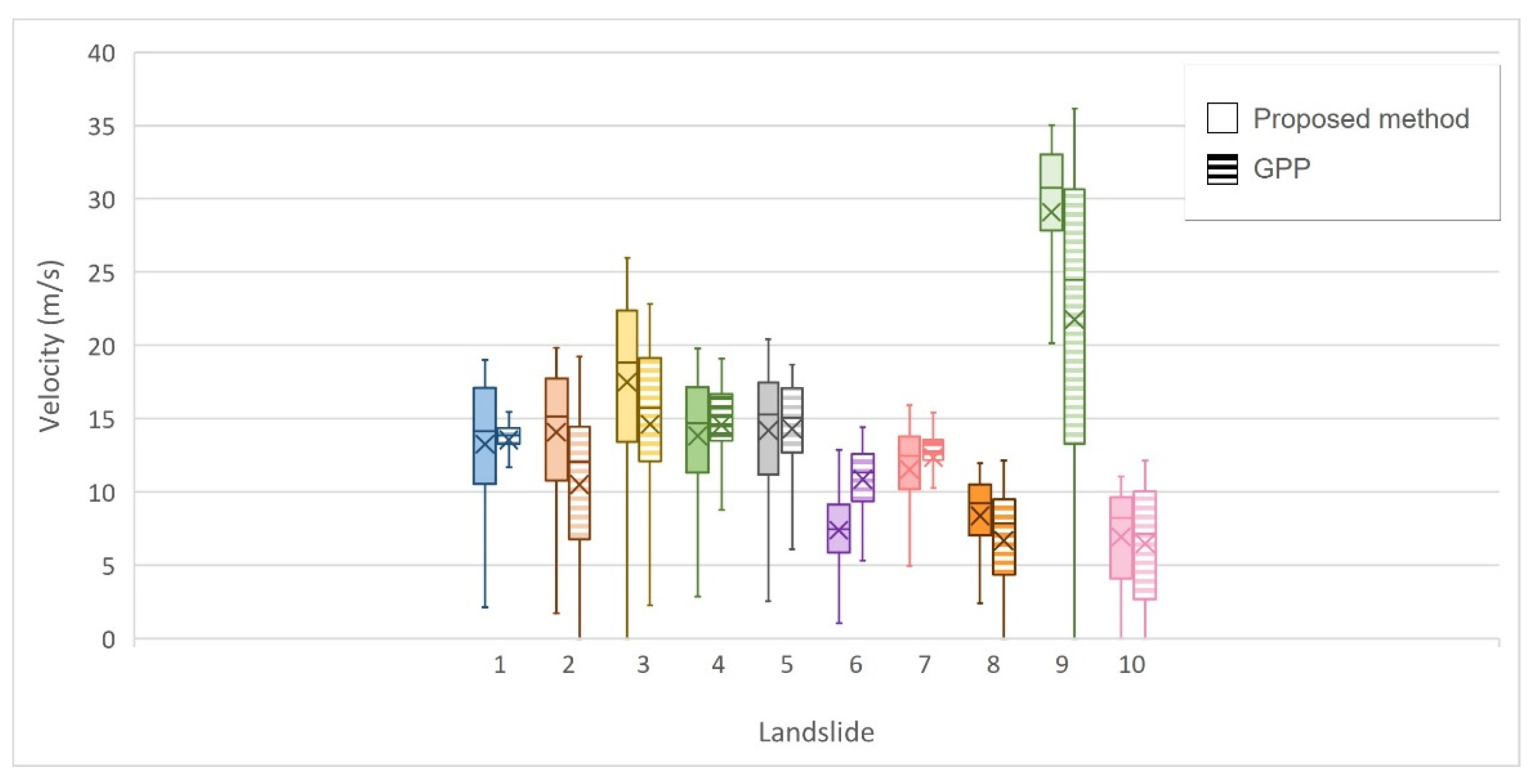
3. Results
Validation of the Results
4. Discussion
5. Conclusions
Supplementary Materials
Author Contributions
Funding
Institutional Review Board Statement
Informed Consent Statement
Data Availability Statement
Conflicts of Interest
References
- Cruden, D.M. A Simple Definition of a Landslide. Bull. Int. Assoc. Eng. Geol. 1991, 43, 27–29. [Google Scholar] [CrossRef]
- Nadim, F.; Kjekstad, O.; Peduzzi, P.; Herold, C.; Jaedicke, C. Global Landslide and Avalanche Hotspots. Landslides 2006, 3, 159–173. [Google Scholar] [CrossRef]
- Cruden, D.M.; Varnes, D.J. Landslides Types and Processes. Landslide: Investigation and Mitigation, Transportation Research Board; Natural Academy Press: Washington, DC, USA, 1994. [Google Scholar]
- Hürlimann, M.; Rickenmann, D.; Medina, V.; Bateman, A. Evaluation of Approaches to Calculate Debris-Flow Parameters for Hazard Assessment. Eng. Geol. 2008, 102, 152–163. [Google Scholar] [CrossRef]
- Jakob, M.; Stein, D.; Ulmi, M. Vulnerability of Buildings to Debris Flow Impact. Nat. Hazards 2012, 60, 241–261. [Google Scholar] [CrossRef]
- Tofani, V.; Del Ventisette, C.; Moretti, S.; Casagli, N. Integration of Remote Sensing Techniques for Intensity Zonation within a Landslide Area: A Case Study in the Northern Apennines, Italy. Remote Sens. 2014, 6, 907–924. [Google Scholar] [CrossRef] [Green Version]
- Solari, L.; Bianchini, S.; Franceschini, R.; Barra, A.; Monserrat, O.; Thuegaz, P.; Bertolo, D.; Crosetto, M.; Catani, F. Satellite Interferometric Data for Landslide Intensity Evaluation in Mountainous Regions. Int. J. Appl. Earth Obs. Geoinf. 2020, 87, 102028. [Google Scholar] [CrossRef]
- Kim, M.-I.; Kwak, J.-H. Assessment of Building Vulnerability with Varying Distances from Outlet Considering Impact Force of Debris Flow and Building Resistance. Water 2020, 12, 2021. [Google Scholar] [CrossRef]
- Novellino, A.; Cesarano, M.; Cappelletti, P.; Di Martire, D.; Di Napoli, M.; Ramondini, M.; Sowter, A.; Calcaterra, D. Slow-Moving Landslide Risk Assessment Combining Machine Learning and InSAR Techniques. Catena 2021, 203, 105317. [Google Scholar] [CrossRef]
- Arattano, M.; Marchi, L. Measurements of Debris Flow Velocity through Cross-Correlation of Instrumentation Data. Nat. Hazards Earth Syst. Sci. 2005, 5, 137–142. [Google Scholar] [CrossRef] [Green Version]
- Dorren, L.K.A.; Berger, F.; le Hir, C.; Mermin, E.; Tardif, P. Mechanisms, Effects and Management Implications of Rockfall in Forests. For. Ecol. Manag. 2005, 215, 183–195. [Google Scholar] [CrossRef]
- Bardi, F.; Raspini, F.; Frodella, W.; Lombardi, L.; Nocentini, M.; Gigli, G.; Morelli, S.; Corsini, A.; Casagli, N. Monitoring the Rapid-Moving Reactivation of Earth Flows by Means of GB-InSAR: The April 2013 Capriglio Landslide (Northern Appennines, Italy). Remote Sens. 2017, 9, 165. [Google Scholar] [CrossRef] [Green Version]
- Duncan, J.M. State of the art: Limit equilibrium and finite-element analysis of slopes. J. Geotech. Eng. 1996, 122, 577–596. [Google Scholar] [CrossRef]
- Pastor, M.; Blanc, T.; Haddad, B.; Petrone, S.; Sanchez Morles, M.; Drempetic, V.; Issler, D.; Crosta, G.B.; Cascini, L.; Sorbino, G.; et al. Application of a SPH Depth-Integrated Model to Landslide Run-out Analysis. Landslides 2014, 11, 793–812. [Google Scholar] [CrossRef] [Green Version]
- Lan, H.; Derek Martin, C.; Lim, C.H. RockFall Analyst: A GIS Extension for Three-Dimensional and Spatially Distributed Rockfall Hazard Modeling. Comput. Geosci. 2007, 33, 262–279. [Google Scholar] [CrossRef]
- Hungr, O. A Model for the Runout Analysis of Rapid Flow Slides, Debris Flows, and Avalanches. Can. Geotech. J. 1995, 32, 610–623. [Google Scholar] [CrossRef]
- Wichmann, V. The Gravitational Process Path (GPP) Model (v1.0)–A GIS-Basedsimulation Framework for Gravitational Processes. Geosci. Model Dev. 2017, 10, 3309–3327. [Google Scholar] [CrossRef] [Green Version]
- Prochaska, A.B.; Santi, P.M.; Higgins, J.D.; Cannon, S.H. A study of methods to estimate debris flow velocity. Landslides 2008, 5, 431–444. [Google Scholar] [CrossRef]
- Carlà, T.; Intrieri, E.; Di Traglia, F.; Nolesini, T.; Gigli, G.; Casagli, N. Guidelines on the Use of Inverse Velocity Method as a Tool for Setting Alarm Thresholds and Forecasting Landslides and Structure Collapses. Landslides 2017, 14, 517–534. [Google Scholar] [CrossRef] [Green Version]
- Corominas, J.; van Westen, C.; Frattini, P.; Cascini, L.; Malet, J.-P.; Fotopoulou, S.; Catani, F.; Van Den Eeckhaut, M.; Mavrouli, O.; Agliardi, F.; et al. Recommendations for the Quantitative Analysis of Landslide Risk. Bull. Eng. Geol. Environ. 2014, 73, 209–263. [Google Scholar] [CrossRef]
- Fell, R.; Corominas, J.; Bonnard, C.; Cascini, L.; Leroi, E.; Savage, W.Z. Guidelines for landslide susceptibility, hazard and risk zoning for land-use planning. Eng. Geol. 2008, 102, 99–111. [Google Scholar] [CrossRef] [Green Version]
- Pudasaini, S.P.; Krautblatter, M. The Landslide Velocity. Earth Surf. Dyn. 2022, 10, 165–189. [Google Scholar] [CrossRef]
- Bayer, B.; Simoni, A.; Mulas, M.; Corsini, A.; Schmidt, D. Deformation Responses of Slow Moving Landslides to Seasonal Rainfall in the Northern Apennines, Measured by InSAR. Geomorphology 2018, 308, 293–306. [Google Scholar] [CrossRef]
- Raspini, F.; Bianchini, S.; Ciampalini, A.; Del Soldato, M.; Solari, L.; Novali, F.; Del Conte, S.; Rucci, A.; Ferretti, A.; Casagli, N. Continuous, Semi-Automatic Monitoring of Ground Deformation Using Sentinel-1 Satellites. Sci. Rep. 2018, 8, 7253. [Google Scholar] [CrossRef] [PubMed] [Green Version]
- Crippa, C.; Valbuzzi, E.; Frattini, P.; Crosta, G.B.; Spreafico, M.C.; Agliardi, F. Semi-Automated Regional Classification of the Style of Activity of Slow Rock-Slope Deformations Using PS InSAR and SqueeSAR Velocity Data. Landslides 2021, 18, 2445–2463. [Google Scholar] [CrossRef]
- Pawluszek-Filipiak, K.; Borkowski, A.; Motagh, M. Multi-Temporal Landslide Activity Investigation by Spaceborne SAR Interferometry: The case study of Polish Carpathians. Remote Sens. Appl. Soc. Environ. 2021, 24, 100629. [Google Scholar] [CrossRef]
- Heim, A. Bergsturz und Menschenleben; Fretz und Wasmuth: Zurich, Switzerland, 1932. [Google Scholar]
- Cignetti, M.; Manconi, A.; Manunta, M.; Giordan, D.; De Luca, C.; Allasia, P.; Ardizzone, F. Taking Advantage of the ESA G-POD Service to Study Ground Deformation Processes in High Mountain Areas: A Valle d’Aosta Case Study, Northern Italy. Remote Sens. 2016, 8, 852. [Google Scholar] [CrossRef] [Green Version]
- Ratto, S.; Giardino, M.; Giordan, D.; Alberto, W.; Armand, M. Carta dei Fenomeni Franosi della Valle d’Aosta; Tipografia Valdostana: Aosta, Italy, 2007. [Google Scholar]
- Trigila, A.; Iadanza, C.; Guerrieri, L. The IFFI Project (Italian Landslide Inventory): Methodology and Results. Guidelines for Mapping Areas at Risk of Landslides in Europe; APAT: Rome, Italy, 2007; pp. 15–18. [Google Scholar] [CrossRef]
- Trigila, A.; Iadanza, C. Landslides in Italy. Special Report; Italian National Institute for Environmental Protection and Research (ISPRA): Rome, Italy, 2008.
- Ratto, S.; Bonetto, F.; Comoglio, C. The October 2000 Flooding in Valle d’Aosta (Italy): Event Description and Land Planning Measures for the Risk Mitigation. Int. J. River Basin Manag. 2003, 1, 105–116. [Google Scholar] [CrossRef]
- Giardino, M.; Giordan, D.; Ambrogio, S.G.I.S. Technologies for Data Collection, Management and Visualization of Large Slope Instabilities: Two Applications in the Western Italian Alps. Nat. Hazards Earth Syst. Sci. 2004, 4, 197–211. [Google Scholar] [CrossRef]
- Cossart, E.; Braucher, R.; Fort, M.; Bourlès, D.L.; Carcaillet, J. Slope Instability in Relation to Glacial Debuttressing in Alpine Areas (Upper Durance Catchment, Southeastern France): Evidence from Field Data and 10Be Cosmic Ray Exposure Ages. Geomorphology 2008, 95, 3–26. [Google Scholar] [CrossRef]
- Martinotti, G.; Giordan, D.; Giardino, M.; Ratto, S. Controlling Factors for Deep-Seated Gravitational Slope Deformation (DSGSD) in the Aosta Valley (NW Alps, Italy). Geol. Soc. Lond. Spec. Publ. 2011, 351, 113–131. [Google Scholar] [CrossRef]
- Crosta, G.B.; Frattini, P.; Agliardi, F. Deep Seated Gravitational Slope Deformations in the European Alps. Tectonophysics 2013, 605, 13–33. [Google Scholar] [CrossRef]
- Canuti, P.; Casagli, N. Considerazioni sulla Valutazione del Rischio di Frana. Fenomeni Franosi e Centri Abitati. Atti del Convegno di Bologna; Consiglio Nazionale delle Ricerche: Rome, Italy, 1996.
- Tarquini, S.; Nannipieri, L. The 10 M-Resolution TINITALY DEM as a Trans-Disciplinary Basis for the Analysis of the Italian Territory: Current Trends and New Perspectives. Geomorphology 2017, 281, 108–115. [Google Scholar] [CrossRef]
- Jahn, J. Entwaldung und Steinschlag. In Proceedings of the International Congress Interpraevent, Graz, Austria, 4–8 July 1988; Volume 1, pp. 185–198. [Google Scholar]
- Zinggeler, A. Steinschlagsimulation in Gebirgswa Ldern: Modellierung der Relevanten Teilprozesse. Master’s Thesis, University of Bern, Bern, Switzerland, 1990; p. 116. [Google Scholar]
- Gsteiger, P. Steinschlagschutzwald. Ein Beitrag zur Abgrenzung, Beurteilung und Bewirtschaftung. Schweiz. Z. Forstwes. 1993, 144, 115–132. [Google Scholar]
- Doche, O. Etude Experimentale de Chutes de Blocs en Forêt. In Cemagref Doc. 97/0898; Cemagref/Institut des Sciences et Techniques de Grenoble (ISTG): Grenoble, France, 1997; p. 130. [Google Scholar]
- Perret, S.; Dolf, F.; Kienholz, H. Rockfalls into Forests: Analysis and Simulation of Rockfall Trajectories -Considerations with Respect to Mountainous Forests in Switzerland. Landslides 2004, 1, 123–130. [Google Scholar] [CrossRef]
- Iverson, R.M. The Physics of Debris Flows. Rev. Geophys. 1997, 35, 245–296. [Google Scholar] [CrossRef] [Green Version]
- Rickenmann, D. Empirical relationships for debris flows. Nat. Hazards 1999, 19, 47–77. [Google Scholar] [CrossRef]
- Goetz, J.; Kohrs, R.; Parra Hormazábal, E.; Bustos Morales, M.; Belén Araneda Riquelme, M.; Henríquez, C.; Brenning, A. Optimizing and Validating the Gravitational Process Path Model Forregional Debris-Flow Runout Modelling. Nat. Hazards Earth Syst. Sci. 2021, 21, 2543–2562. [Google Scholar] [CrossRef]
- Perla, R.; Cheng, T.T.; McClung, D.M. A two-parameter model of snow-avalanche motion. J. Glaciol. 1980, 26, 197–207. [Google Scholar] [CrossRef] [Green Version]
- Salvatici, T.; Tofani, V.; Rossi, G.; D’Ambrosio, M.; Tacconi Stefanelli, C.; Masi, E.B.; Rosi, A.; Pazzi, V.; Vannocci, P.; Petrolo, M.; et al. Application of a physically based model to forecast shallow landslides at a regional scale. Nat. Hazards Earth Syst. Sci. 2018, 18, 1919–1935. [Google Scholar] [CrossRef] [Green Version]
- D’Ambrosio, M.; Tofani, V.; Rossi, G.; Salvatici, T.; Tacconi Stefanelli, C.; Rosi, A.; Masi, E.B.; Pazzi, V.; Vannocci, P.; Catani, F.; et al. Application of regional physically-based landslide early warning model: Tuning of the input parameters and validation of the results. In EGU General Assembly Conference Abstracts; EGU: Munich, Germany, 2017; p. 13712. [Google Scholar]
- Hungr, O. Dynamics of Rapid Landslides. In Progress in Landslide Science; Springer: Berlin/Heidelberg, Germany, 2007; pp. 47–57. [Google Scholar] [CrossRef]
- Bellugi, D.G.; Milledge, D.G.; Cuffey, K.M.; Dietrich, W.E.; Larsen, L.G. Controls on the size distributions of shallow landslides. Proc. Natl. Acad. Sci. USA 2021, 118, e2021855118. [Google Scholar] [CrossRef]


Publisher’s Note: MDPI stays neutral with regard to jurisdictional claims in published maps and institutional affiliations. |
© 2022 by the authors. Licensee MDPI, Basel, Switzerland. This article is an open access article distributed under the terms and conditions of the Creative Commons Attribution (CC BY) license (https://creativecommons.org/licenses/by/4.0/).
Share and Cite
Marinelli, A.; Medici, C.; Rosi, A.; Tofani, V.; Bianchini, S.; Casagli, N. Shallow Landslides and Rockfalls Velocity Assessment at Regional Scale: A Methodology Based on a Morphometric Approach. Geosciences 2022, 12, 177. https://0-doi-org.brum.beds.ac.uk/10.3390/geosciences12040177
Marinelli A, Medici C, Rosi A, Tofani V, Bianchini S, Casagli N. Shallow Landslides and Rockfalls Velocity Assessment at Regional Scale: A Methodology Based on a Morphometric Approach. Geosciences. 2022; 12(4):177. https://0-doi-org.brum.beds.ac.uk/10.3390/geosciences12040177
Chicago/Turabian StyleMarinelli, Antonella, Camilla Medici, Ascanio Rosi, Veronica Tofani, Silvia Bianchini, and Nicola Casagli. 2022. "Shallow Landslides and Rockfalls Velocity Assessment at Regional Scale: A Methodology Based on a Morphometric Approach" Geosciences 12, no. 4: 177. https://0-doi-org.brum.beds.ac.uk/10.3390/geosciences12040177