

Integrated Schumann Resonance Intensity as an Indicator of the Global Thunderstorm Activity
1
Hayakawa Institute of Seismo Electromagnetics Co., Ltd. (Hi-SEM), UEC Alliance Center #521, 1-1-1 Kojima-cho, Chofu-shi, Tokyo 182-0026, Japan
2
Advanced Wireless & Communications Research Center (AWCC), The University of Electro-Communications (UEC), 1-5-1 Chofugaoka, Chofu-shi, Tokyo 182-8585, Japan
3
Department of Applied Mathematics and Control Processes, Saint-Petersburg State University, 35, University Ave., Peterhof, Saint-Petersburg 198504, Russia
4
O.Ya. Usikov Institute for Radio-Physics and Electronics, National Academy of Sciences of the Ukraine, 12, Acad. Proskura Street, 61085 Kharkov, Ukraine
*
Author to whom correspondence should be addressed.
Geosciences 2023, 13(6), 177; https://0-doi-org.brum.beds.ac.uk/10.3390/geosciences13060177
Submission received: 24 April 2023
/
Revised: 30 May 2023
/
Accepted: 13 June 2023
/
Published: 14 June 2023
(This article belongs to the Topic Advances in Environmental Remote Sensing)
Abstract
:This paper addresses the accuracy of estimates for the contemporary level of global thunderstorm activity found from the synchronous records of integrated Schumann resonance (SR) intensity at two high-latitude observatories in the Northern and Southern hemispheres. The results are based on numerical simulations of electromagnetic fields in the frequency band of the global (Schumann) resonance in the Earth–ionosphere cavity characterized by a realistic conductivity profile in the middle atmosphere. The credible distribution is used for global thunderstorm activity in space and time. The paired observatory locations are considered either at the geographic poles or at Svalbard and the Antarctic Peninsula. The seasonal variations in the spatial distribution of global thunderstorms are adopted from the OTD satellite observations. The diurnal variations imply the spatial and temporal distribution of lightning strokes measured by the WWLLN network for an arbitrarily chosen date of 18 January 2022. The results obtained suggest that simultaneous records of the integrated SR intensity at Svalbard and in Antarctica provide errors below 3% in the diurnal variations of global thunderstorm activity with a temporal resolution of 10 min. The seasonal changes in global thunderstorm intensity are estimated with an error of ~10%. Since the level of global thunderstorm activity varies by a factor of two on the both time scales, the estimates confirm the appropriate accuracy of the estimate of thunderstorm activity from the concurrent measurements at the high-latitude SR observatories in the Arctic and Antarctic.
1. Introduction
Geoscience incorporates three great areas corresponding to three media: the solid earth, the ocean, and the Earth’s atmosphere. The present paper is concerned with the terrestrial atmosphere, namely, it addresses the global electric activity of the Earth’s atmosphere.
It is well known that the global electromagnetic (Schumann) resonance in the Earth–ionosphere cavity is driven by electromagnetic radiation from global thunderstorms. Schumann resonance (SR) and its observations are described in detail in the literature. The necessary information and the bibliography may be found in previous works [1,2,3,4,5,6,7,8]. SR is observed in the vertical electric or (more often) in the horizontal magnetic field. Power spectra of global SR have maxima (modes) at frequencies of 8, 14, 20 Hz, etc., and the resonance intensity might be used for estimating the level of global lightning activity. The major obstacle to such measurements arises from the distance dependence of the modal amplitudes. The latter emerges in the closed spherical Earth–ionosphere cavity bounded by the ground surface and the lower ionosphere. This is why the amplitude of the recorded oscillations varies non-monotonously with the source–observer distance: the field amplitude acquires the maxima and minima in space arising from the interaction of the direct and antipodal waves propagating through the cavity. For compensating spatial variations, an application was proposed of the total resonance intensity, i.e., the spectral density integrated over the frequency band covering several resonance modes [1,9,10,11,12].
Usually, the power spectral density is integrated over the first three modes: from about 5 to 23 Hz. The quantitative estimates for the accuracy of this technique were discussed in [10] in a realistic Earth–ionosphere cavity model when excited by a point vertical dipole source. It was shown that frequency integration reduces deviations in the estimated source intensity from ~6 dB to a level of about 1 dB. Unfortunately, these estimates were relevant only to a compact field source, while actual thunderstorm activity covers substantial areas over the globe. Thus, it is highly desirable to obtain similar estimates for the actual position and size of global thunderstorms relative to the observer. The demand for such a study becomes especially obvious from a recent study based on multi-stationed SR observations [13]. In this context, the modeling is necessary of simultaneous SR monitoring at globally separated observatories. This particular subject is the goal of the present study.
2. Formulation of the Problem
We apply the uniform Earth–ionosphere cavity model: a spherical cavity uniform along the angular coordinates, which is formed by the perfectly conducting ground and the horizontally stratified atmosphere of conductivity gradually increasing with height. We use the vertical profile of air conductivity suggested in [14]. This profile is used in the full-wave solution for computing the propagation constant of extremely low frequency (ELF) radio waves υ(f) and the normalizing factor N(f); they both depend on the signal frequency f as seen in [14,15,16,17]. Since two orthogonal components of the horizontal magnetic field are usually recorded in experimental observations, we use the west–east HWE = HX and the south–north HSN = HY components. These fields are formally described by the zero-order mode of the Earth–ionosphere waveguide at ELF. The power spectra of these fields are described by the following expressions [5]:
Each sum in Equations (1) and (2) accounts for the mutually independent lightning strokes, which are distributed over the Earth’s surface. The following notations are used: a is the Earth’s radius; N(f) is the normalization coefficient (the excitation factor); υ(f) is the propagation constant; is the associated Legendre function of the complex index υ; θi is the angular distance from the observer to the i-th lightning stroke; Azi denotes the particular source azimuth at the observation point; Mi is the current moment of the i-th discharge.
Equations (1) and (2) describe the accumulation of pulsed power arriving from the individual lightning strokes. These relations are valid when the global thunderstorms form the Poisson succession of ELF radio pulses. Such an assumption is quite natural, since the random individual lightning discharges are mutually independent.
3. Model Daily Variations
For introducing the model daily variations in the level of global lightning activity, one must specify the coordinates and occurrence times of particular lightning strokes. These data are used in our computations of the SR intensity. The real records of the World Wide Lightning Location Network (WWLLN) are well suited for this purpose. The network operates in the very low frequency (VLF) band [18,19,20,21,22]. The relative closeness of the WWLLN operating frequency band 6–18 kHz to the SR band of 4–40 Hz serves in favor of utilizing these data in modeling of the global electromagnetic resonance signals. The WWLLN exploits the observation sites covering the entire globe, which synchronously register the pulses arriving from the lightning discharges. The network data provide the occurrence time of particular strokes and their coordinates derived from the mutual delay of pulses arriving at different sites. The radiated energy is also estimated by WWLLN [18,19,20,21,22].
The computations are organized in the following way. As the first step, we find the source–observer distance and the arrival angle (source bearing) of particular radio pulse by using known position of lightning strokes. We compute the SR power spectra in two orthogonal components of the horizontal magnetic field at the observatory. In Equations (1) and (2), we account for the radiated energy of a stroke provided by the WWLLN. In fact, we assume that the spectral density radiated by a lightning stroke being directly proportional to |Mi|2 is independent of frequency (the source current moments have the ‘white’ spectra).
We selected an arbitrary date of the WWLLN record for our modeling, 18 January 2022. Prior to calculating the SR power spectra, we inspected the WWLLN data and eliminated the pulses with energy significantly exceeding the typical level in the data set; the reason for these deviations remains unknown (reading error?). In order to demonstrate general features of the WWLLN data, we show in Figure 1 the spatial distribution of lightning strokes in the time interval 12:00–13:00 UTC. This figure presents the world map in the rectangular projection. Geographic longitude and latitude are plotted in degrees along the abscissa and ordinate. The map outlines the continents. Positions of all 28,703 lightning strokes are shown in the figure by the red diamonds. One may observe that the majority of lightning strokes appear southward of the equator, which reflects the seasonal drift of global thunderstorm activity. The strokes are often detected over land, and discharges concentrate around Indonesia, Australia, South Africa, Madagascar, and South America during this particular time interval. All these features agree with climatology data on the global thunderstorm distribution.
We divided the original record of the WWLLN network into 10-min intervals, for which the field components were computed and the contributions accumulated of individual lightning strokes into the SR power spectra. Thus, the 144 cumulative power spectra were obtained in two orthogonal magnetic field components at an arbitrary observatory during the day. To obtain estimates of the contemporary intensity of SR oscillations (over 10 min), we integrated the power spectra over the frequency band 5–23 Hz with a step of 0.1 Hz. The integrated spectra of individual field components were then summed, providing the integrated power of the total horizontal magnetic field as seen below.
Energy radiated by the lightning activity according to WWLLN data was also summed over the same 10-min time intervals thus providing the level of the ongoing intensity of global thunderstorms. This value was compared with the integrated intensity of SR.
It is clear that the integrated intensity of SR at a site will slightly increase when global thunderstorms approach the observer and decrease when the thunderstorms move away from him. It is necessary to somehow compensate for this remaining distance-dependence of the integrated spectral power. The simplest way is to use the simultaneous records at a couple of ‘conjugate’ observatories located in such a way that the observed increase in the intensity at one point is compensated by an equal decrease at the other field site.
3.1. Polar Observers
One may expect that the most promising pair of observatories should occupy the geographic North and South Poles. We know that global thunderstorm activity is concentrated at low latitudes. We may expect therefore that the diurnal drift of thunderstorms around the globe will not cause considerable alterations in the source distance from a polar observatory. Simultaneously, a moderate decrease in the distance from one observer will be compensated by relevant increase from the other one. Consequently, the sum of the integrated SR intensities recorded at the poles will be insensitive to the daily movement of lightning activity: this sum will adequately reflect alterations in the level of global thunderstorm activity.
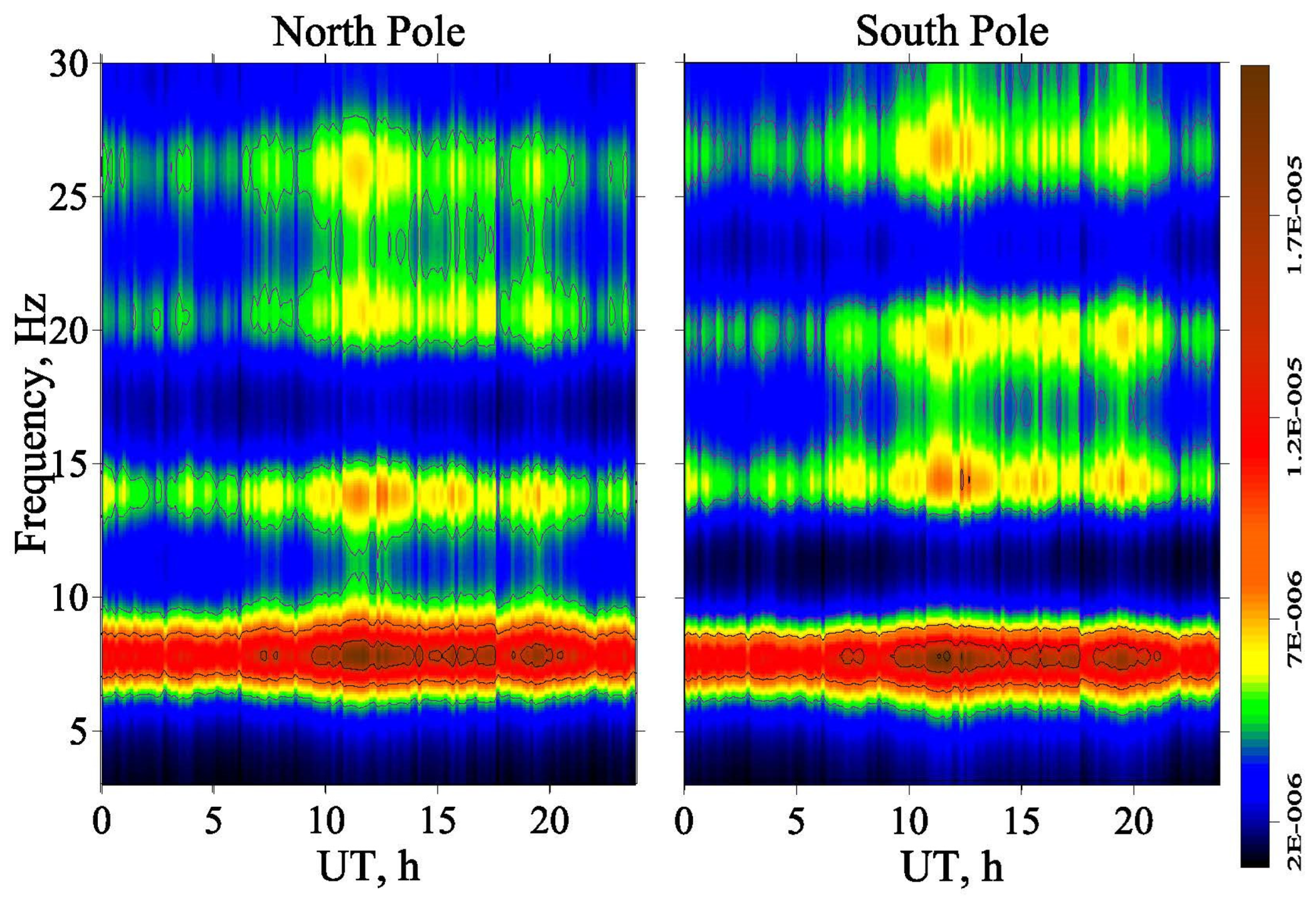
Figure 2 demonstrates the simulated dynamic power spectra of the total horizontal magnetic field in the SR band. Daily variations in the spectra were computed for observers positioned at the North (left panel) and South Pole (right panel). The horizontal axis shows the Universal Time (UT) in hours, and the vertical axis depicts the frequency in Hertz. The total magnetic field power is shown by the color, and the common color scale is found to the right of the dynamic spectra.
A remark is appropriate here that the term ‘west–east direction’ has no sense at the poles. We postulated that the HSN field component is directed along the Greenwich zero meridian, while the orthogonal HWE component is orthogonal to it.
The spectral peaks of the global electromagnetic resonance are visible in the dynamic spectra as the horizontal yellow-red stripes in the vicinity of 8, 14, 20, 26 Hz. These areas are separated by the dark-blue bands corresponding to the minima in the power spectral density. The figure illustrates a high similarity of the dynamic spectra at the opposite poles of the Earth, although the resonance intensity is slightly higher at the South Pole than at the North Pole. The general outline of the SR pattern indicates their close relationship to the diurnal variations in the thunderstorm activity rather than to their positions.
We show in Figure 3 the temporal changes in the cumulative intensities of resonance oscillations: the power spectral density and integrated over the frequency band 5–23 Hz with a step of 0.1 Hz. Individual curves in Figure 3 show the power spectra integrated over the frequency, i.e., along the vertical lines in Figure 2. The abscissa in Figure 3 shows the UT in hours, and the integrated intensity is plotted along the ordinate in relative units. The red curves in this figure correspond to the South Pole data, and the blue curves show the data from the North Pole.
The left panel in Figure 3 shows temporal changes in the integrated intensity of separate field components west–east and south–north. The right panel allows us to compare diurnal variations in the total horizontal magnetic field H at the poles. These plots demonstrate the degree of mutual similarity of the curves calculated for the opposite poles.
Diurnal variations in the intensity of the HWE field at both poles have a clear maximum in the vicinity of the UTC noon. In contrast, the power of HSN component has a minimum in this time interval. It shows an increase occurring around 20:00 UTC, and the smaller local maxima are present in the interval 0–4:00 and around 10:00 UTC. The maxima are easily explained. The growth in the HWE component is conditioned by the increase in thunderstorm activity in Madagascar and South Africa, which is natural for the boreal winter. This activity reaches its maximum around the UTC noon hours. The maxima in the intensity of the orthogonal HSN field component are associated with the thunderstorms in South America (20 h), Oceania (0–4 h), and Southeast Asia with Australia (10 h). Hence, the temporal behavior of these fields is conditioned by the above-chosen orientation of magnetic field components at the poles.
It is important to note that SR signals at the South Pole slightly exceed those detected at the North Pole. These variations indicate that the distance-dependence in the integrated field intensity was not completely compensated by applying the frequency-integrated individual field components.
The right panel in Figure 3 depicts the SR power in the total horizontal magnetic field at the North and the South Poles. The total magnetic field power is characterized by a single wide daily maximum at both the polar sites. The maximum is located in the vicinity of 11–12 h UTC. Obviously, the residual effect of the varying source–observer distance might be further reduced by summing the integrated SR intensities observed at the poles. The results of such an operation are presented in Figure 4.
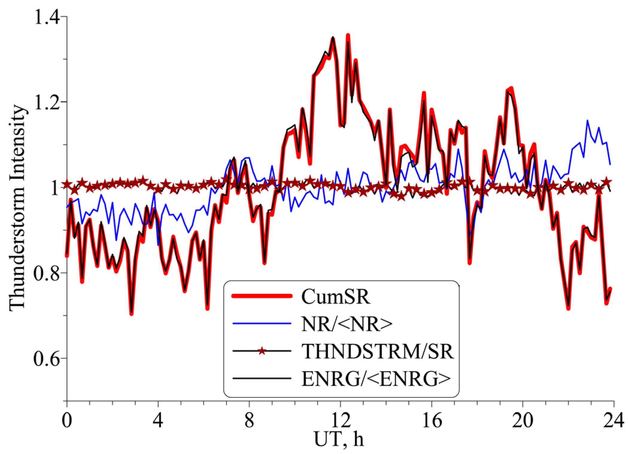
Figure 4 shows the diurnal changes of the following values obtained in the model computations. The thin blue curve depicts variations of the normalized number of lightning strokes recorded during each 10-min interval by the WWLLN network on 18 January 2022. From now on, the angular brackets denote the averaging over the day. The thin black line shows changes in time of the normalized total energy emitted by the global lightning strokes also corresponding to every 10-min interval of observations by WWLLN. The bold red curve originates from the SR data: it depicts the normalized cumulative resonance intensity at the North and South Poles . It is clear that the black and the red lines in Figure 4 are practically coincident, i.e., the cumulative SR power in the polar records follows in time the energy radiated by the global lightning activity.
The black curve with brown stars illustrates the accuracy of the measurement technique: this is the ratio of the normalized energy radiated by the lightning strokes to the normalized cumulative intensity of SR. The daily mean of this ratio is equal to 1.0004, and its standard deviation is 0.9%. Thus, the results of numerical modeling bring us to the conclusion that simultaneous records of SR at the North and South Poles allow for accurate monitoring of changes in the level of global thunderstorm activity on the daily scale.
3.2. Diurnal Variations for High-Latitude Observers
After completing the modeling of diurnal variations at the Earth’s poles, let us turn to more realistic records at the coupled high-latitude observatories in the Arctic and Antarctic. These should be equipped with the same calibrated receiving hardware and exploit the same processing technique. There is such a pair of facilities: the Ukrainian Antarctic Observatory “Akademik Vernadsky” (UAS; 65.25° S and 64.24° W) and the Norwegian observatory on Svalbard SOUSY (78.15° N and 16.05° E); the details can be found in [23,24].
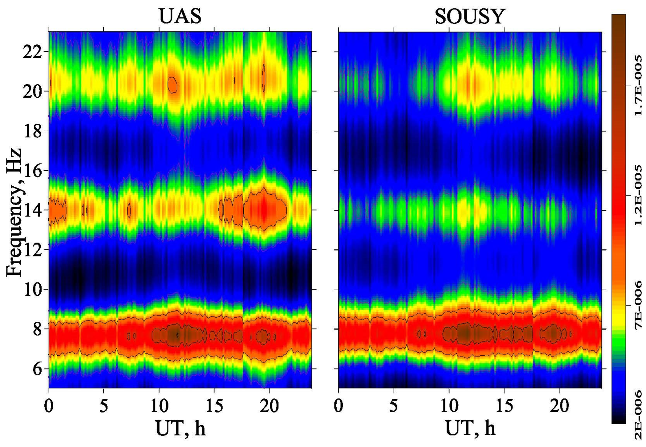
Figure 5 shows the model dynamic spectra of SR computed for these two observatories and based on the WWLLN thunderstorm data for the same date of 18 January 2022. We computed the power spectra of the HWE and HSN horizontal magnetic field components and obtained afterwards the power spectra of the total magnetic field relevant to the 10-min tine intervals. These dynamic power spectra of total field H at UAS and SOUSY are shown in Figure 5 as the 2D maps above the time–frequency plane. The abscissas in both panels depict the UTC in hours, and the ordinate displays the ELF frequency in Hertz. The power spectral density of the total horizontal magnetic field is shown by color and the corresponding color scale is placed on the right. The Arctic and the Antarctic spectrograms are found on the right and left panels of Figure 5.
The SR peaks are clearly visible at the sub-polar field sites in form of the horizontal red and yellow bands. The spectral minima separating the peaks are outlined by dark-blue horizontal areas. The spectrograms demonstrate that diurnal variations in the global resonance intensity have much in common at each observatory. One may notice the maximum in the intensity of electromagnetic signal in the vicinity of UTC noon present both in the Arctic and Antarctic sites. At the same time, definite variations are observed and the resonance intensity in the Arctic is slightly smaller than that in the Antarctic. The disparities arise from the longitudinal separation of the field sites by almost 90° and by the winter displacement of global thunderstorms into the Southern hemisphere.
Figure 6 shows temporal variations of the cumulative intensity of SR oscillations similarly to Figure 4: the power spectral density integrated in the frequency band 5–23 Hz. The abscissas here show the UT in hours, and the ordinate depicts the integrated resonance intensity in arbitrary units. The red curves in this figure correspond to the data from the Southern hemisphere, and the bluish curves are relevant to the Northern hemisphere.
The left panel of Figure 6 demonstrates temporal changes in the integrated intensity of the south–north field component HSN of the horizontal magnetic field. The plots showing diurnal variations of the integrated intensity of the west–east component HWE and of the total horizontal magnetic field H occupy the right panel of Figure 6. The south–north field component is noticeably smaller than the west–east component, which is explained by the problem geometry: the particular spatial distribution of lightning strokes. One may conclude that in this particular case of the sub-polar position of observatories, an outstanding similarity is observed of the model curves relevant to the total field and to the west–east component computed in opposite hemispheres.
The west–east and south–north components at the high latitudes in the Arctic and Antarctic demonstrate a comprehensive increase in resonance intensity during the time intervals of high lightning activity at the global thunderstorm centers in Madagascar and South Africa (around 12 h) and in South America (20 h). The influence of thunderstorms in Oceania (0–4 h) and Southeast Asia including Australia (10 h) is less pronounced than that observed at the polar observatories. As a whole, variations at the high-latitude sites significantly deviate from the patterns computed for the poles. However, the resonance signals in the Antarctic slightly exceed those in the Arctic again, which indicates that the distance-dependence in the integrated field intensity was not compensated completely.
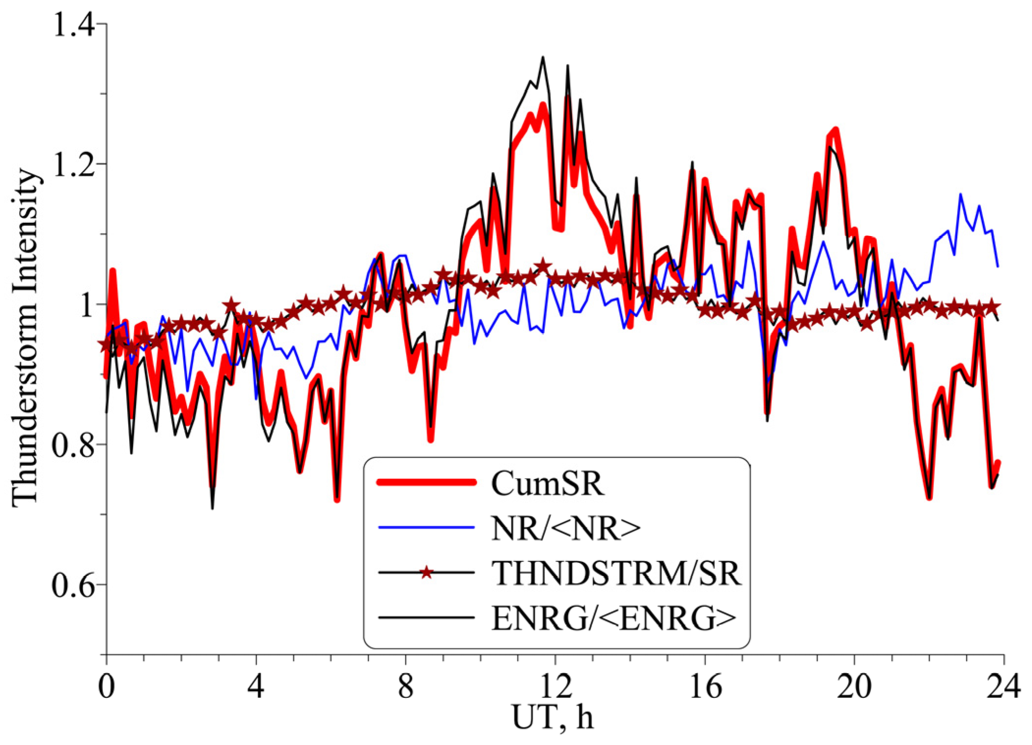
Figure 7 compares the diurnal changes in the level of global thunderstorm activity (global lightning radiated power) and the cumulative SR intensity. The legend in Figure 7 is similar to that of Figure 5. The blue curve depicts the normalized variations of the number of lightning strokes recorded by the WWLLN in each 10-min interval of 18 January 2022. The black curve shows changes in the normalized radiated energy ENRG/<ENRG> of all lightning discharges summed during every 10-min interval. The thick red curve shows changes in the normalized cumulative integrated SR intensity at the SOUSY and UAS sites. The black curve with brown stars outlines the daily changes in the ratio of the normalized cumulative SR intensity and the normalized lightning energy. The scheme of this figure repeats the arrangement used in Figure 5.
Similarly to speculative positioning of the observers at the poles, the computations for the existing high-latitude observatories indicate that the cumulative intensity of the global electromagnetic resonance is almost coincident with the daily variations in the radiation energy of global thunderstorm activity. One may observe that the black curve with brown stars in Figure 7 does not essentially deviate from the constant equal to unity. Its daily median value is equal to 0.998, and the standard deviation is equal to 2.7%. Thus, the simultaneous records of SR at the currently operating high-latitude observatories SOUSY and UAS allow for accurate estimating of the level of global thunderstorm activity on the time scales of 10 min or higher.
4. Model Seasonal Variations
Let us model the seasonal variations in global thunderstorm activity and its reflection in the SR records performed at different observation sites. To model the spatial distribution of the field sources, we use the monthly averaged maps of global thunderstorm activity according to the OTD (Optical Transient Detector) satellite observations [25]. These data have the form of tables for each month of the year, averaged over several years of orbital observations. We divide the entire globe along latitude and longitude into cells of the size of 2.5° by 2.5°. Global lightning activity is proportional to the average number of lightning flashes observed in a particular cell during a given month for the entire observation period.
A figure showing all 12 maps with the spatial distribution of global thunderstorms for each month turns out to be very cumbersome. Therefore, we present in Figure 8 only maps for the four seasons of the year: for the periods December–January–February, March–April–May, June–July–August, and September–October–November. The geographic longitude is plotted in degrees along the abscissa on these maps, and the latitude is shown along the ordinate. The spatial distribution of lightning flashes is shown by the color. One may easily recognize the continents outlined by the spatial distribution of lightning strokes. The north–south and west–east seasonal grifts are visible in these maps of global thunderstorm activity.
In computations, we use the coordinates of the center of the corresponding cell of 2.5° by 2.5° as the position of the elementary source. The radiated power of such an elementary source is considered to be directly proportional to the number of optical lightning flashes observed in this cell. By moving from cell to cell, we calculate the geometric parameters of elementary propagation paths (the source–observer distance and the arrival angle of the radio wave at the observation point) and compute by using Equations (1) and (2) the power spectra of individual field components and of the total horizontal magnetic field at a given observatory for each month of a year.
Such an approach is not a great novelty: the similar spatial distribution of global thunderstorm activity was taken into account 50 years ago in the paper [26]. The significant distinction of the present study is that in [26] the yearly averaged distribution of the ‘thunder days’ over the Earth’s surface was used, i.e., the days in a year when the sound of thunder was heard at a given meteorological station (see [27]). To model the daily changes in global thunderstorm activity, the authors of [26] used a standard sinusoidal ‘modulation factor’ depending on time, by which they multiplied the number of thunder days within the longitude sectors of the 15° width. This product of the spatial thunderstorm distribution and of the temporal modulating factor provided the model diurnal variations. In the previous part of this study, we used the updated diurnal variations based on the actual global observations of lightning strokes by the WWLLN.
To model seasonal changes, we apply 12 maps of the global distribution of lightning flashes observed aboard the OTD satellite during each month and averaged over the whole period of its observations [25]. A detailed description of applying the OTD data in the SR computations may be found in [6,11,12].
One may expect that the integrated intensity of SR will slightly increase when the global thunderstorms come closer to an observer and will decrease when the thunderstorms drift away from him. As we note before, the simplest way to compensate for this remnant distance-dependence is to simultaneously monitor the integrated resonance intensity at two observatories located such that an increase in the intensity at one of them is combined with its corresponding decrease at the other site.
When treating seasonal variations, we initially consider positioning of the coupled observatories at the North and the South Poles. As might be seen from the maps of Figure 8, global thunderstorm activity is always confined to low latitudes. Therefore, one might expect that a decrease in the distance from one observer will be compensated by its increase relative to another one during the seasonal drift of thunderstorms relative to polar observatories. Then, the sum of the integrated power measured at the poles should be insensitive to the seasonal drift of global thunderstorms and will tend to reflect alterations in the intensity of global thunderstorm activity.
4.1. Polar Observers
We show in Figure 9 the model spectrograms of the total horizontal magnetic field power in the SR band. Seasonal variations in the power spectra of the total magnetic field were computed using the monthly OTD maps for observers positioned at the South (left panel) and the North Pole (right panel). The abscissa shows the month of the year, and the ordinate depicts the frequency of SR radio signal in Hertz. The total field power is shown by color, and the color scale is positioned at the right of the dynamic spectra.
The spectra on the seasonal scale acquire an outline deviating of spectra in Figure 2 and Figure 5. The major distinction is in the ‘isolated’ summer peaks especially visible as the spots at the higher modes. As in the case of diurnal variations, the northern and southern spectrograms remain similar in spite of the fact that the computations were made for the opposite poles of the Earth. The behavior of resonance intensity at the poles is close, but not coincident. Deviations in the general resonance pattern at the observatories indicate the traces of their link to the source–observer distance, which is different owing to seasonal displacements of global thunderstorm activity.
Figure 10 shows separately the monthly averaged power spectra of SR in the total horizontal magnetic field at the North and the South Poles. The frequency in Hertz is plotted along the abscissa, and the power spectral density in relative units is plotted along the ordinate. The spectra for January are shown by the black lines, and those for July are shown by the red lines. The data for the South Pole are marked with red circles, and those for the North Pole are marked with blue circles.
The spectra in Figure 10 demonstrate a pronounced resonance pattern, and some details might be seen in a more vivid manner than in the plots in Figure 9. The resonance peaks in the power spectra corresponding to the first three resonance modes are clearly visible. The resonance intensity tends to decrease when the distance to the source increases. In addition, a slight deformation of the spectra as a whole is also visible, which alters the form of resonance curve and the heights of individual peaks. Therefore, the seasonal changes in the outline of resonance spectra at the Poles are not coincident. In contrary to optimistic expectations, the seasonal drifts in the global thunderstorm position provide changes at a pole that could not be completely compensated by changes at the other pole even in the integrated power spectra.
Validity of this conclusion is clearly demonstrated in Figure 11. Months are plotted along the abscissa and the intensity of SR and of global thunderstorms is plotted along the ordinate in relative units. All data shown in this figure were normalized in such a way that their annual mean value was equal to 100.
The thin blue line with blue circles depicts the seasonal variations in the integrated SR intensity at the North Pole. The thin red line with red circles shows the simultaneous seasonal changes in the integrated SR intensity at the South Pole. As might be seen, the polar seasonal changes are highly similar in spite of some variations in details. In particular, the intensity of the SR noticeably increases at both hemispheres during the boreal summer. The thick black line with black circles corresponds to the half-sum of the integrated intensities at the North and the South Pole. It occupies an intermediate position between the individual curves relevant to the poles.
The bold blue line in Figure 11 shows the seasonal variations in the monthly mean of the global thunderstorm activity observed by the OTD satellite. We have scaled the data so that the annual average values became equal to 100, and this involves the blue line and the thick black line with black dots. After such scaling, these two lines would become coincident in an ideal case. Unfortunately, this did not happen. We observe that seasonal variations in the SR intensity are more pronounced than alterations in the thunderstorm activity following from the orbital optical observations.
When comparing the seasonal model data, we acted in the following way. First, we calculated the yearly average MSR = < PSR >, where PSR is the half-sum of integrated SR intensities detected at the poles during particular month. We computed similarly the yearly average of global thunderstorm activity MTh = < STh >, where STh is directly proportional to the cumulative number of global lightning strokes observed by OTD during a month. The median values MSR and MTh allow us to obtain the normalized seasonal variations of both parameters and . The accuracy of estimating the seasonal changes of global thunderstorm activity by using SR records is equal to the ratio of the normalized seasonal variations .
The bold black line with brown stars described as Poles/OTD in the legend of Figure 11 shows the sought seasonal variation ratio . This curve illustrates relative deviations of global thunderstorm activity derived from the SR records against the “actual” intensity of global lightning activity recorded by OTD. The assessment of the level of global thunderstorm activity by using the half-sum of the integrated SR power at the North and the South Pole deviates from the postulated thunderstorm activity by +20 and –11%, depending on the particular month. (The annual means of these data are coincident by default.)
The observed variations are apparently associated with an uneven distribution of thunderstorms along the longitude and with their seasonal drift along the latitude and the longitude. These features are related to the geographical allocation of continents in the Northern and Southern hemispheres because thunderstorms tend to concentrate over solid land. The resulting estimate allows us to speak about a modest evaluation accuracy of the global thunderstorm level based on the concurrent ELF observations at the poles.
Since, according to OTD data, the amount of lightning stokes varies by a factor of two depending on the season, the polar observers provide a modest accuracy in assessing the seasonal changes in the level of global thunderstorms. Unfortunately, it is impossible to apply the above results in practice, since there are no sites monitoring the SR at the terrestrial poles. Therefore, we return to modeling the observations at the existing operating couple of high-latitude sites: UAS (65.25° S and 64.24° W) and SOUSY (78.15° N and 16.05° E).
4.2. High-Latitude Observers in the Northern and Southern Hemispheres
We present below the model seasonal results for UAS and SOUSY points based on the OTD maps. Using the power spectra of the orthogonal west–east and south–north components, we find the power spectra of the total magnetic field for each month of a year. These spectra are shown in Figure 12 as the 2D maps above the month–frequency plane.
The abscissas in Figure 12 show the months, and the frequency of the signal is plotted along the ordinate. The power spectral density is shown by color, and the corresponding color scale is placed on the right. Resonance peaks are clearly visible, and the seasonal changes in the SR intensity are well resolved at each observatory. There is a pronounced increase in the intensity of electromagnetic signal recorded both in the Arctic and Antarctic during the boreal summer. Simultaneously, the relative summer intensity increase in the Arctic exceeds that in the Antarctic, which is explained by the distance-dependence of the resonance field. The major conclusion that might be drawn from Figure 12 is that SR observations at any of the hemispheres reflect seasonal changes in the level of global thunderstorm activity. Since the magnitude of seasonal changes in the SR intensity in the Northern hemisphere significantly exceeds the changes in the Southern hemisphere, the realistic estimate of global thunderstorms must imply the half-sum of the resonance powers observed in both the hemispheres.
Figure 13 shows seasonal variations of the integrated SR intensity at the two sub-polar sites. The interval of 12 months’ duration is shown along the abscissa in Figure 13, and the resonance intensity is plotted in arbitrary units along the ordinate. The blue line with blue dots represents the Arctic data (Svalbard) and the red line with red dots shows the Antarctic observations (Antarctic Peninsula). The bold black line with the black asterisks presents the half-sum of the Arctic and Antarctic data. The bold blue line outlines changes in global thunderstorm activity, which is directly proportional to the mean number of planetary lightning strokes observed from orbit during a given month. The seasonal changes are obviously similar in global thunderstorm activity and in the half-sum of integrated SR intensities at the high-latitude observatories.
As before, we derive the ratio of the seasonal variations in the SR to changes in the OTD record . Here, is the normalized cumulative SR intensity and denotes the normalized global thunderstorm activity in the OTD data. This ratio is depicted by the black bold line with the brown stars in Figure 13. It indicates that in the framework of the OTD global thunderstorm distribution, the simultaneous monitoring of SR at the high latitude Arctic and Antarctic stations allows estimation of the contemporary level of global thunderstorm activity with an accuracy ranging from −6 to +10%. This result confirms the fortunate positioning of these particular observatories, which facilitates the remote sensing of changes in the current global thunderstorm activity with an error of about ±10% on the annual time scale.
5. Summary
- The numerical simulations showed a rather high accuracy of the estimates for the diurnal variations in the level of global thunderstorm activity by using the concurrent records of the integrated SR intensity at two high-latitude observatories, UAS and SOUSY. The relative error does not exceed 3% for the daily time resolution of 10 min or more;
- Alterations in the relative intensity of global thunderstorms on the seasonal time-scale are estimated from the SR data with an error of about 10%;
- Since the rate of changes in the level of global thunderstorm activity on the considered time-scales is approximately one octave (the factor of two), the above errors indicate an acceptable overall accuracy of the estimates acquired using simultaneous SR monitoring at the high-latitude observatories in the Arctic and Antarctic.
6. Conclusions
Geoscience studies the processes that occur in the three media, being the solid Earth, the ocean, and the Earth’s atmosphere. The present work is addressed to one of these media: to the terrestrial atmosphere. We model and discuss the scheme of possible remote sensing of the level of global thunderstorm activity by using the natural electromagnetic radiation from the lightning strokes captured in the Earth–ionosphere cavity. Model computations indicate that the global electromagnetic (Schumann) resonance might serve as a reliable tool for such measurements, provided that ELF radio signals are concurrently monitored in the Northern and the Southern Hemispheres at high-latitude or at polar observatories.
We must emphasize that the modeling procedure has used the particular realistic planetary distributions of lightning strokes. Of course, the generalization of the estimates obtained to reality may seem ambiguous, since particular random distributions might deviate from those used in the model. Nevertheless, we dare to express an optimistic opinion that the actual relative errors will not cross the corridor of 10% width. This belief is supported by the fact that the models applied were based on modern observations of thunderstorm activity.
The model data obtained indicate that concurrent high-latitude ELF measurements in the Northern and the Southern Hemispheres will allow adequate estimates for the diurnal and seasonal patterns in the level of global thunderstorm activity to be obtained.
Author Contributions
Conceptualization, M.H. and A.P.N.; Methodology, Y.P.G. and A.P.N.; Software, Y.P.G. All authors have read and agreed to the published version of the manuscript.
Funding
This research received no external funding.
Institutional Review Board Statement
Not applicable.
Informed Consent Statement
Not applicable.
Data Availability Statement
All data can be provided by the corresponding author upon request.
Acknowledgments
The authors are grateful to the colleagues of WWLLN for providing us with the data.
Conflicts of Interest
The authors declare no conflict of interest.
References
- Polk, C. Relation of ELF noise and Schumann resonances to thunderstorm activity. In Planetary Electrodynamics; Coronoti, S.C., Hughes, J., Eds.; Gordon and Breach: New York, NY, USA, 1969; Volume 2, pp. 55–83. [Google Scholar]
- Polk, C. Schumann resonances. In Handbook of Atmospherics; Volland, H., Ed.; CRC Press: Boca Raton, FL, USA, 1982; Volume 1, pp. 111–178. [Google Scholar]
- Bliokh, P.V.; Nickolaenko, A.P.; Filippov, Y.F. Schumann Resonances in the Earth-Ionosphere Cavity; Peter Perigrinus: New York, NY, USA; London, UK; Paris, France, 1980; p. 168. [Google Scholar]
- Sentman, D.D. Schumann Resonances. In Handbook of Atmospheric Electrodynamics; Volland, H., Ed.; CRC Press: Boca Raton, FL, USA; London, UK; Tokyo, Japan, 1995; Volume 1, pp. 267–298. [Google Scholar]
- Nickolaenko, A.P.; Hayakawa, M. Resonances in the Earth-Ionosphere Cavity; Kluwer Academic Publishers: Dordrecht, The Netherlands, 2002; p. 388. [Google Scholar]
- Nickolaenko, A.; Hayakawa, M. Schumann Resonance for Tyros; Springer: Tokyo, Japan; Heidelberg, Germany; New York, NY, USA; Dordrecht, The Netherlands; London, UK, 2014; p. 348. [Google Scholar] [CrossRef]
- Price, C. ELF electromagnetic waves from lightning: The Schumann resonances. Review. Atmosphere 2016, 7, 116. [Google Scholar] [CrossRef] [Green Version]
- Nickolaenko, A.P.; Shvets, A.V.; Hayakawa, M. Propagation at Extremely Low-Frequency Radio Waves. In Wiley Encyclopedia of Electrical and Electronics Engineering; Webster, J., Ed.; John Wiley & Sons, Inc.: Hoboken, NJ, USA, 2016; pp. 1–20. [Google Scholar] [CrossRef]
- Sentman, D.D.; Fraser, B.J. Simultaneous observation of Schumann resonances in California and Australia: Evidence for intensity modulation by local height of D. region. J. Geophys. Res. 1991, 96, 15973–15984. [Google Scholar] [CrossRef]
- Nickolaenko, A.P. Modern aspects of the Schumann resonance studies. J. Atmos. Solar-Terr. Phys. 1997, 59, 805–816. [Google Scholar] [CrossRef]
- Nickolaenko, A.P.; Hayakawa, M.; Sekiguchi, M. Variations in global thunderstorm activity inferred from the OTD records. Geophys. Res. Lett. 2006, 33, L06823. [Google Scholar] [CrossRef]
- Sekiguchi, M.; Hayakawa, M.; Nickolaenko, A.P.; Hobara, Y. Evidence of a link between the intensity of Schumann resonance and global surface temperature. Ann. Geophys. 2006, 24, 1809–1817. [Google Scholar] [CrossRef] [Green Version]
- Bozóki, T.; Sátori, G.; Williams, E.; Guha, A.; Liu, Y.; Steinbach, P.; Leal, A.; Atkinson, M.; Beggan, C.D.; DiGangi, E.; et al. A Schumann Resonance-based quantity for characterizing day-to-day changes in global lightning activity. J. Geophys. Res. Atmos. 2023; in press. [Google Scholar] [CrossRef]
- Kudintseva, I.G.; Nickolaenko, A.P.; Rycroft, M.J.; Odzimek, A. AC and DC global electric circuit properties and the height profile of atmospheric conductivity. Ann. Geophys. 2016, 59, A0545. [Google Scholar] [CrossRef]
- Hynninen, E.M.; Galuk, Y.P. The field of vertical electric dipole source over the spherical Earth with non-uniform along the height ionosphere. In Problems of Radio Wave Diffraction and Propagation; LSU Publ.: St. Petersburg, Russia, 1972; pp. 109–120. [Google Scholar]
- Galuk, Y.P.; Ivanov, V.I. Propagation characteristics of VLF fields in the waveguide Earth–vertically non-uniform anisotropic ionosphere. In Problems of Radio Wave Diffraction and Propagation; LSU Publ.: St. Petersburg, Russia, 1978; pp. 148–153. [Google Scholar]
- Galuk, Y.P. Schumann resonance in the model of global thunderstorm activity uniformly distributed over the Earth. Radio-Phys. Electron. 2015, 6, 3–9. [Google Scholar]
- Lay, E.H.; Rodger, C.J.; Holzworth, R.H.; Dowden, R.L. Introduction to the World Wide Lightning Location Network (WWLLN). Geophys. Res. Abstr. 2005, 7, 02875, 2005 SRef-ID: 1607-7962/gra/EGU05-A-02875. [Google Scholar]
- Rodger, C.J.; Werner, S.; Brundell, J.B.; Lay, E.H.; Thomson, N.R.; Holzworth, R.H.; Dowden, R.L. Detection efficiency of the VLF World-Wide Lightning Location Network (WWLLN): Initial case study. Ann. Geophys. 2006, 24, pp. 3197–3214. Available online: www.ann-geophys.net/24/3197/2006 (accessed on 10 January 2023).
- Hutchins, M.L.; Holzworth, R.H.; Brundell, J.B.; Rodger, C.J. Relative detection efficiency of the World Wide Lightning Location Network. Radio Sci. 2012, 47, RS6005. [Google Scholar] [CrossRef]
- Rodger, C.J.; Brundell1, J.B.; Hutchins, M.; Holzworth, R.H. The world wide lightning location network (WWLLN): Update of status and applications. In Proceedings of the 2014 XXXIth URSI General Assembly and Scientific Symposium (URSI GASS), Beijing, China, 16–23 August 2014. [Google Scholar] [CrossRef]
- Holzworth, R.H.; Brundell, J.B.; McCarthy, M.P.; Jacobson, A.R.; Rodger, C.J.; Anderson, T.S. Lightning in the Arctic. Geophys. Res. Lett. 2021, 48, e2020GL091366. [Google Scholar] [CrossRef]
- Koloskov, A.V.; Bezrodny, V.G.; Budanov, O.V.; Yampolski, Y.M. Polarization monitoring of the Schumann resonances in the Antarctic and recognition of the world thunderstorm activity characteristics. Radiofiz. I Radioastron. 2005, 10, 11–29. [Google Scholar]
- Koloskov, O.V.; Nickolaenko, A.P.; Yampolski, Y.M.; Budanov, O.V. Electromagnetic seasons in Schumann resonance records. J. Geophys. Res. Atmos. 2022, 127, e2022JD036582. [Google Scholar] [CrossRef]
- Christian, H.J.; Blakeslee, R.J.; Boccippio, D.J.; Boeck, W.L.; Buechler, D.E.; Driscoll, E.T.; Goodman, S.J.; Hall, J.M.; Koshak, W.J.; Mach, D.M.; et al. Global frequency and distribution of lightning as observed from space by the Optical Transient Detector. J. Geophys. Res. 2003, 108, 4005. [Google Scholar] [CrossRef] [Green Version]
- Ogawa, T.; Murakami, Y. Schumann resonance frequencies and conductivity profiles in the atmosphere. Contr. Geophys. Inst. Kyoto Univ. 1973, 13, 13–20. [Google Scholar]
- Israel, H. Atmospherische Elekrizitat; Akademische Verlaggeseltschaft: Leipzig, Germany, 1961; Volume 2, 503p. [Google Scholar]
Figure 1.
Spatial distribution of lightning discharges (red dots) over the globe according to the WWLLN data for the interval 12–13 h UTC on 18 January 2022.
Figure 1.
Spatial distribution of lightning discharges (red dots) over the globe according to the WWLLN data for the interval 12–13 h UTC on 18 January 2022.

Figure 2.
Dynamic spectra of SR for observers at the geographic North and South Poles.

Figure 3.
Daily variations of the integrated intensity of the field components (left panel) and the total horizontal magnetic field (right panel) at the North and the South Poles.
Figure 3.
Daily variations of the integrated intensity of the field components (left panel) and the total horizontal magnetic field (right panel) at the North and the South Poles.

Figure 4.
Diurnal variations of the sum of the integrated SR intensities at the poles and changes in the parameters of global lightning activity.
Figure 4.
Diurnal variations of the sum of the integrated SR intensities at the poles and changes in the parameters of global lightning activity.

Figure 5.
Model dynamic spectra of SR at high-latitude observatories in the Arctic and Antarctic.

Figure 6.
Daily variations in the integrated intensity of horizontal magnetic fields computed for the Arctic and Antarctic observatories.
Figure 6.
Daily variations in the integrated intensity of horizontal magnetic fields computed for the Arctic and Antarctic observatories.

Figure 7.
Diurnal variations in the cumulative integral intensities of SR observed in the Arctic and Antarctic, changes in the stroke rate and in the global lightning radiated power.
Figure 7.
Diurnal variations in the cumulative integral intensities of SR observed in the Arctic and Antarctic, changes in the stroke rate and in the global lightning radiated power.

Figure 8.
Global distribution of lightning discharges in four annual seasons.

Figure 9.
Annual spectrograms of the total horizontal magnetic field of SR computed for the South and North Poles.
Figure 9.
Annual spectrograms of the total horizontal magnetic field of SR computed for the South and North Poles.

Figure 10.
Model SR spectra at the North and South Poles in January and July.

Figure 11.
Seasonal changes in the integral SR intensity at the North and the South Pole compared with the level of global thunderstorms according to the OTD observations.
Figure 11.
Seasonal changes in the integral SR intensity at the North and the South Pole compared with the level of global thunderstorms according to the OTD observations.

Figure 12.
SR spectrograms at the UAS and SOUSY observatories.

Figure 13.
Estimated seasonal variations in global thunderstorm activity found from observations at the high-latitude observatories.
Figure 13.
Estimated seasonal variations in global thunderstorm activity found from observations at the high-latitude observatories.

Disclaimer/Publisher’s Note: The statements, opinions and data contained in all publications are solely those of the individual author(s) and contributor(s) and not of MDPI and/or the editor(s). MDPI and/or the editor(s) disclaim responsibility for any injury to people or property resulting from any ideas, methods, instructions or products referred to in the content. |
© 2023 by the authors. Licensee MDPI, Basel, Switzerland. This article is an open access article distributed under the terms and conditions of the Creative Commons Attribution (CC BY) license (https://creativecommons.org/licenses/by/4.0/).
Share and Cite
MDPI and ACS Style
Hayakawa, M.; Galuk, Y.P.; Nickolaenko, A.P. Integrated Schumann Resonance Intensity as an Indicator of the Global Thunderstorm Activity. Geosciences 2023, 13, 177. https://0-doi-org.brum.beds.ac.uk/10.3390/geosciences13060177
AMA Style
Hayakawa M, Galuk YP, Nickolaenko AP. Integrated Schumann Resonance Intensity as an Indicator of the Global Thunderstorm Activity. Geosciences. 2023; 13(6):177. https://0-doi-org.brum.beds.ac.uk/10.3390/geosciences13060177
Chicago/Turabian StyleHayakawa, Masashi, Yuriy P. Galuk, and Alexander P. Nickolaenko. 2023. "Integrated Schumann Resonance Intensity as an Indicator of the Global Thunderstorm Activity" Geosciences 13, no. 6: 177. https://0-doi-org.brum.beds.ac.uk/10.3390/geosciences13060177
Note that from the first issue of 2016, this journal uses article numbers instead of page numbers. See further details here.