Article

Comparing Flow-R, Rockyfor3D and RAMMS to Rockfalls from the Mel de la Niva Mountain: A Benchmarking Exercise

1
Risk Analysis Group, Institute of Earth Sciences, University of Lausanne, CH-1015 Lausanne, Switzerland
2
Geohazard and Earth Observation Team, Earth Surface and Seabed Division, Geological Survey of Norway (NGU), NO-7491 Trondheim, Norway
3
Rambøll Norge AS, NO-7493 Trondheim, Norway
4
BEG SA, CH-1994 Aproz (Nendaz), Switzerland
5
Norbert SA, Engineering Geology and Hydrogeology, CH-1920 Martigny, Switzerland
6
Natural Hazards Study Laboratory (LERN), Department of Geology and Geological Engineering, Laval University, Québec City, QC G1V 0A6, Canada
*
Author to whom correspondence should be addressed.
Submission received: 5 January 2023 / Revised: 5 May 2023 / Accepted: 26 June 2023 / Published: 30 June 2023
(This article belongs to the Special Issue Rockfall Protection and Mitigation)

Abstract

:
Rockfall simulations are often performed at various levels of detail depending on the required safety margins of rockfall-hazard-related assessments. As a pseudo benchmark, the simulation results from different models can be put side-by-side and compared with reconstructed rockfall trajectories, and mapped deposited block fragments from real events. This allows for assessing the objectivity, predictability, and sensitivity of the models. For this exercise, mapped data of past events from the Mel de la Niva site are used in this paper for a qualitative comparison with simulation results obtained from early calibration stages of the Flow-R 2.0.9, Rockyfor3D 5.2.15 and RAMMS::ROCKFALL 1.6.70 software. The large block fragments, reaching hundreds of megajoules during their fall, greatly exceed the rockfall energies of the empirical databases used for the development of most rockfall models. The comparison for this challenging site shows that the models could be improved and that combining the use of software programs with different behaviors could be a workaround in the interim. The findings also highlight the inconvenient importance of calibrating the simulations on a per-site basis from onsite observations. To complement this process, a back calculation tool is briefly described and provided. This work also emphasizes the need to better understand rockfall dynamics to help improve rebound models.

1. Introduction

The back analysis and trajectory reconstruction of rockfall events, such as those covered in the companion publication Noël et al. [1], provide valuable data for the important calibration of rockfall simulations (Jones et al., [2]; Labiouse, [3]; Berger and Dorren, [4]; Berger et al., [5]; Volkwein et al., [6]; Dorren et al., [7]; Valagussa et al., [8]; Bourrier et al., [9]; Noël et al., [10]). Simulations are often performed with various levels of detail with associated calibrations depending on the required level of certainty and safety margins. Since the required resources increase with the complexity of the required level of detail, rockfall hazards are often approached in different stages. As described in detail by Hantz et al. [11], Volkwein et al. [6], Jaboyedoff et al. [12] and Loup and Dorren [13], the typical stages where simulations are performed with an approximative increasing order of required certainty are as follows:
  • Rockfall susceptibility/indicative hazard evaluations;
  • Quantitative rockfall hazard zoning;
  • Detailed risk assessment related to rockfalls;
  • Mitigation measure designs.
First, the susceptibility stage is meant to quickly cover large regions with conservative safety margins. This ensures that only the areas, for which it is not possible to fall within any of the subsequent rockfall hazard zone classes, would be phased out at this stage. Geometrical methods are commonly used for delimiting the envelopes of areas that are potentially reachable by rockfalls at that stage, given their high efficiency to perform at a regional scale with grid-based/GIS-based approaches (Dorren, [14]; topographic–hydrologic approaches in Volkwein et al., [6]; Michoud et al., [15]). Such derived models can be expressed geometrically with the propagation defined from the reach angle, sometime called energy line or Fahrböschung, obtained from the expected horizontal and vertical distance travelled by the rocks. The alpha–beta model (Domaas, [16]), CONEFALL’s model (Jaboyedoff and Labiouse, [17]) and Flow-R’s simplified friction-limited model (Horton et al., [18]) are examples of such geometrical models. A rough estimation of the kinetic energies can also be obtained geometrically from these methods by considering the potential energy of the height difference (Δh) between the terrain elevation and the reach angle line, or the cone for a given rock mass and gravitational acceleration (g) (Jaboyedoff and Labiouse, [17]). Pseudo velocities (vpseudo) without rotation can also be roughly estimated in the same way with Equation (1) (modified from Dorren et al. [7]) as follows:
v p s e u d o = 2 g h ,
However, these first geometric estimations should be distinguished from the process-based methods, sometimes called “dynamic” or “trajectographic” methods, often required in the subsequent stages (ONR 24810, [19]; OFEV, [20]; Mölk and Rieder, [21]; Direktoratet for byggkvalitet, [22]; NVE, [23]; Loup and Dorren [13]). With the constantly improving processing capabilities of computers, some have already transitioned toward using process-based methods at the susceptibility stage for potentially more realistic predictions with simulated behaviors closer to a rockfall’s modes of motion. For examples, Frattini et al. [24], Noël [25], Dupire et al. [26], Kalsnes et al. [27], Alvioli et al. [28], Alvioli et al. [29] and Dorren et al. [30] ran process-based simulations in batches with models derived from Pfeiffer and Bowen [31] to obtain billions of simulated rockfall trajectories over Norway, the Alps, and hundreds of kilometers of railways in Italy and Canada.
Given the large safety margins ensuring long runouts that would cover all subsequent hazard zone classes, the calibration process is rather simple at the susceptibility stage. As conceptualized in Figure 1, the simulated envelope should include most of the observed/mapped deposited rockfall blocks for the covered region. One should be careful at this stage to keep enough margin to account for the lack of per-site calibrations from field observations and an oversimplification of the simulated rockfall’s modes of motion depending on the simulation models used.
The quantitative rockfall hazard zoning and risk assessment of the second and third stages (E2 and E3 in OFEV, [20]) are well described by Jaboyedoff et al. [12], Volkwein et al. [6], Hantz et al. [11] and Loup and Dorren [13]. For a reference period, the spatial-temporal hazard probability is defined by the product of the probability of failure of a rock mass generating rock fragments within a given reference volume/energy range and the probabilities of the rock fragments reaching exposed objects while they propagate downslope. As covered by Jaboyedoff et al. [12] and Hantz et al. [11] and conceptualized in Figure 1d, it is important to choose the proper width of influence of the simulated trajectories combined with the exposed “reachable” objects or the proper related cell size of the gridded results since this has a great effect on the obtained reach probabilities. As the distance from a rockfall source increases, the propagation probabilities decrease not only because the rocks gradually come to rest but also because their lateral spreading gradually covers a wider area (Evans and Hungr, [32]; Jaboyedoff et al. [12]). It is therefore important that a model reproduces the mapped observed lateral deviations to obtain proper propagation and reach probabilities for quantitative use. Simulating a series of small samples of trajectories (e.g., 20–50) helps with performing the plausibility check by easing the visualization of each individual trajectory, as conceptualized with the yellow paths compared to the hypothetical mapped observed paths in red (Figure 1). A model producing overly channelized results, unless matching with the observations, should be fine-tuned further.
For rockfall hazard zoning, risk assessments or the design of mitigation measures, kinetic energies (intensities) are usually required to determine the vulnerability of the exposed infrastructure/building objects, and the population and capacity of the mitigation measures (Raetzo et al. [33]; Jaboyedoff et al. [12]; Volkwein et al. [6]; Lambert and Bourrier, [34]; Lambert et al. [35]). The simulations must then be calibrated at those stages to reproduce the observed kinetic energies. Additionally, since results can vary greatly from user to user (Berger et al. [36]; Berger and Dorren, [4]; Berger et al. [5]; Garcia, [37]; C2ROP, [38]), having real observations as a reference for calibration reduces potential user biases. Domaas [39], Descoeudres [40], Volkwein et al. [6], Wyllie [41] and Gerber [42] detail how analytical methods can be used to estimate the translational kinetic energies and bounce heights from the positions of a succession of impact marks and/or combined with the incident angle imprint in the ground at the impacts. These positions can also be determined on 3D detailed terrain models from the imprint impact marks, as in Caviezel et al. [43] and Noël et al. [1]. If video footage from previous rockfall events is available, these values can be reconstructed as well as the rock trajectory segments, as in Noël et al. [44] and Noël et al. [1], for example.
No matter what rockfall hazard stage is involved, it is important to be knowledgeable about the simulation models used, their predictability, sensitivity to different parameters, and objectivity (e.g., Lambert et al. [45]; Lambert and Bourrier, [34]). To evaluate these attributes and eventual limitations, the model’s results can be put side-by-side and compared with observed reconstructed rockfall paths and mapped deposited blocks from real events or rockfall experiments. For a relevant comparison in a practice context, equivalent time resources should ideally be spent per model and close to what is usually spent when delivering projects. With finite resources, the more time reserved to fine-tune the simulations from less predictable and slow software, the less available time there is for the preceding important data collection from field observations. Therefore, one must be careful when sharing perfectly matching simulation results to the rockfall community. These potentially site-dependent results can be misleading if the time spent for the precise calibration or how far the model needs to be pushed beyond its anticipated parameters to reproduce reality is not mentioned. Instead, one can better communicate the predictability, sensitivity, and objectivity of the simulation models by comparing their simulation results at an early calibration stage.
For this exercise, the historical events from Mel de la Niva Mountain, whose 3D trajectories and 2D paths were reconstructed in detail in the companion publication by Noël et al. [1], are used as references in this paper. The 200 m3 blocks, reaching hundreds of megajoules during their fall, greatly exceeded the common rockfall energies of the empirical databases used for the development of most rockfall models (Noël et al. [1]). Such a site can thus be challenging for the simulation models tested in this paper. For a pseudo benchmark with the historical events, preliminary simulation results from the Flow-R 2.0.9 simplified friction-limited geometrical model (Horton et al., [18]), Rockyfor3D 5.2.15 process-based model (Dorren, [46]) and RAMMS::ROCKFALL 1.6.70 process-based model (Leine et al. [47]) are qualitatively compared here. Similarities and discrepancies between the results and a comparison with the reconstructed trajectories are then discussed. As the simulations can be further fine-tuned, and the models can evolve and improve over time, the reader is encouraged to repeat and extend such back analysis calibrations and comparisons. The reconstructed paths and trajectories for this site are shared in CC BY 4.0 in Noël et al. [48], and swissAlti3D elevation models are openly and freely available from ©swisstopo. A back calculation tool is also briefly described following the benchmarking simulations and provided as Supplementary Material to help the reader repeat this comparison analysis on other sites.

2. Benchmarking Approach

For the simulations, the elevation terrain models (DTMs) were prepared with the 2013 DTM from the swissAlti3D product by ©swisstopo. It was resampled by average to the recommended cell size of 10 m for the simulations with Flow-R, and 2 m for Rockyfor3D and RAMMS. The parameters attributed to the terrain (Figure 2) for the three rounds of simulations are summarized in Table 1. They are ordered from left to right following the order in which the simulations were performed. This corresponds to increasing induced runout distances with Flow-R and RAMMS, which both started with too short runouts. For Rockyfor3D, the first simulation was performed with the rapid automatic simulation parameters and was followed by rougher surfaces to reduce the induced runouts.

2.1. Flow-R 2.0.9 Methodology

The parameters of the first scenario with Flow-R correspond to the finalized fine-tuned ones used for a regional analysis in a nearby valley sharing similar terrain features (Michoud et al. [15]). The second scenario uses the same parameters but with a desired reach angle (“basal flow friction”) of 31° that corresponds to the H/L value of 0.6 in Corominas [50], and to reach angles of rockfalls from mountainsides with heights from 100 m and up to 350 m in Domaas [16]. The last scenario uses a reach angle of 25° since the reconstructed trajectories show that the blocks had relatively stable velocities for slopes around that angle (Noël et al. [1]). A pseudo velocity cutoff of 30 m s−1 was added to the last scenario to restrict its runouts that otherwise tend to follow the downstream path of the river at the bottom of the valley. All 2D simulations with this software were performed as in Michoud et al. [15] using the original diffusive flow direction by the gridded groundwater hydrological runoff model from Holmgren [51] with an exponent of 1 that produces highly diffusive flow paths equivalent to that of Quinn et al. [52]. The clever addition of the height factor to emulate debris flow thickness for a diffusion that can pass over small obstacles by Horton et al. [18] was kept to 0 m. The diffuse flow pathways were refined by using the gridded debris flow model from Gamma [53] implemented in Flow-R. As this model is not based on rockfall dynamic processes, there are no parameters related to the rock shapes, sizes or volumes.
For a visual comparison of simulated paths from Flow-R with the reconstructed trajectories from the Mel de la Niva events (Noël et al. [1]), we produced overlaying pseudo paths and deposited blocks based on Horton et al. [18]. Five paths per scenario were simulated using a random walk approach following the probabilistic flow direction distributions used by Flow-R. With this approach, a high number of random walk paths would converge to the same results as those produced with Flow-R. The same corresponding parameters as the original Flow-R simulations were used to obtain the same runout area envelopes. Preparing the input layers, adjusting the parameters and running the different Flow-R simulations were performed in less than an hour thanks to the simplicity and efficiency of the model.

2.2. Rockyfor3D 5.2.15 Methodology

For Rockyfor3D, preparing the terrain model and the five corresponding source layers took approximately 15 min. The four other required layers were generated based on the slope thresholds used by the rapid automatic simulations and the roughness of the site detailed in Noël et al. [10]. The open-source automation tools developed for assessing the rockfall potential along 260 km of railway during the ParaChute project (Noël, [25]; Cloutier et al. [54]; Cloutier et al. [55]) were used to automatically generate the terrain material layers for the three scenarios in approximately 15 min. The d1-d2-d3 dimensions of block 2, 11.1-8.5-4.0 m, were used with an ellipsoid shape by Rockyfor3D, which estimates the inertia value for the simulations. Each scenario was run two times, once with 10,000 trajectories to produce the runout area envelopes and once again to randomly extract five trajectories to be compared to the observed paths for an insight into the simulated propagation and reach probabilities. The whole process was completed in less than an hour thanks to the automation tools and the efficiency of the model.

2.3. RAMMS::ROCKFALL 1.6.70 Methodology

For RAMMS, block 2 was first converted to a .pts file to be used as a real input shape by the software. The 3D model of the block, aligned on its principal axes of inertia, was subsampled by space to a total of 72 points, which is slightly higher than the included shapes with the software. It was then built as a custom block in RAMMS while limited to 263 metric tons due to software restrictions of 100 m3. This block was used for the two first scenarios and simplified to a corresponding ellipsoid for the last scenario to see the effect of the simplified shape. The block was converted to an ellipsoid with the same d1-d2-d3 dimensions, subsampled by space to a total of 82 points and converted to a .pts file for the last scenario. These conversions and building custom blocks in RAMMS took approximately half an hour.
For the first scenario, the same terrain parameters previously used by the WSL Institute for Snow and Avalanche Research SLF to roughly simulate the 2015 Mel de la Niva rockfall event (Lu et al. [49]) were used. They were combined with no initial velocity and an automatic offset to the source cliff. Then, because most simulated blocks stopped a few hundred meters from the source, the terrain parameters were changed to values based on the terrain types described in the user manual: matching scree slopes and mountain meadows with their corresponding parameter. This produced short runout results similar to those of the first scenario, so this was not kept as a second scenario. Then, more realistic runouts were obtained by giving an initial horizontal velocity of 10 m s−1. This could be partly justified by the toppling behavior of the failure but was discarded, as the other software did not require these additional adjustments of their default initial conditions. The hardness of the terrain material was raised instead, setting the scree to the parameter for hard bedrock and the mountain meadow to the parameter for hard rock scree. This helped increase the runouts for the last two scenarios. Surprisingly, a 100 m3 non-flat block (real_equant_1.2.pts) with the same parameters as the two last scenarios significantly increases the runouts (see the simulation results dataset in Noël et al. [48]). For the last scenario, only the shape of the block was changed to the corresponding ellipsoid based on the dimensions of block 2, keeping the same hard material surfaces.
Each scenario was run two times, once with 1000 trajectories to produce the runout area envelopes and once again to randomly extract five trajectories to be compared to the observed paths for an insight into the simulated propagation and to reach probabilities. The maximum number of simulations per scenario had to be reduced from 10,000 to 1000 due to excessive processing time, as more than one night was needed to simulate 10,000 trajectories for this large site while keeping the time step and “dump” step to 0.01 and 0.02 s, respectively. The RAMMS simulations were thus completed in approximately one day, including the fine-tuning work but not counting the first attempt for 10,000 simulations. Without considering license costs, the reader should bear in mind that for a fair comparison in terms of resources, the time spent with RAMMS should have been limited to the same time spent as the others, or the other way around. Also, the simulations should have been performed with the same computing hardware. However, this was not feasible given the license availability.

2.4. Localized Reach Probability and Hazard

To complement the raw simulated results for the comparison, they are also expressed in terms of quantified localized reach probability and guiding hazard zones. The results of the second scenarios are used for that purpose. Note that being expressed in those terms does not improve the preliminary nature of the simulated results limited by their early calibration stage. This is only done here for comparison purposes to help highlight by how much similar simulations would miss the natural phenomena if one overlooks the important fine-tunning steps from field observations. For a relative comparison from one to another, the temporal aspect must be the same for the three software programs. A finalized temporal estimation for the site is, however, not required for this comparison exercise from early calibrated simulations. Given the mass of the reference block scenario of 500 metric tons, the energies involved when the blocks are in movement (at >1.1 m s−1) fall in the highest intensity level of the Swiss danger zonation matrix (combining hazard on the x axis to the corresponding intensity on the y axis). Thus, no emphasis is made related to the intensities or protective effect of the forest for this relative comparison.
For a punctual source, the probability of an exposed object to be reached by a rockfall can be evaluated by summing up the number of unique trajectories that intercept the object and exceed the intensity level at which the object is vulnerable. As mentioned in the introduction (Figure 1d), the dimensions of the object and those of the simulated rock fragment must be considered (Jaboyedoff et al. [12]; Corominas et al. [56]; Hantz et al. [11]). The local reach probability of the object (Pr) is then obtained by dividing the obtained number of intercepting trajectories by the total number of simulated trajectories from the given source.
For simulation models considering the fragmental aspect, a unique trajectory must include the branching segments of its fragments (e.g., HY-STONE from Agliardi and Crosta, [57]; Crosta and Agliardi, [58]; Frattini et al. [24]; EG4 Risk, [59] or RockGIS from Matas et al., [60]). This way, numerous fragments intercepting the exposed object only count as one occurrence if they are related to a common unique trajectory. In that case, the temporal aspect (λ) should be attributed to an expected yearly frequency of failure events from the source (before fragmentation).
The temporal aspect can also be expressed as a yearly frequency of block fragments, for example, estimated from deposited block inventories (Evans and Hungr, [32]) or mapped past trajectory segments (after fragmentation). In that case, the number of trajectories intercepting the exposed object should be estimated from unique trajectories individualized for each simulated fragment. The parent segments starting from the source should be duplicated until their number matches with the number of fragments.
The latter situation can be approximated with simulation models that do not account for the fragmental aspect, like for the software tested. Each simulated trajectory corresponds to a simulated fragment. The effect of this simplification is marginal when the fragmentation is estimated to happen in the vicinity of the source. However, one must remember that the fragmentation induces changes in shape, size and volume of the propagating blocks. Thus, their initial propagating characteristics and related intensities are different than those of the final fragments, which is not accounted for by the simplified simulations.
For an object exposed to numerous (diffuse) sources, rather than evaluating its local reach probability (Pr), it is more appropriate to estimate its local average expected frequency (λobject) of being intercepted by trajectories with exceeding intensities. For that purpose, a fraction of λ must be attributed to each unique trajectory, ideally expressed as a ratio of the corresponding source surface area covered (not the 2D planimetric surface). Additionally, this ratio has the positive side effect of compensating for the strong biases associated with planimetric gridded source distributions (Figure 3 in Noël et al. [10]). For example, if 10,000 trajectories are simulated from a 1000 m2 cliff from 100 sources evenly spread (without grid bias for simplicity), each trajectory corresponds to 0.1 m2, and each source covers 10 m2. Assuming a rockfall event produces 20 fragments in average for that site, an expected yearly λ of 0.2 failure events for that cliff would correspond to a yearly λ of 4 fragments per 1000 m2 cliff in average. Therefore, each source would carry a yearly λ of 0.04 fragments for its 10 m2, which would be subdivided to its 100 related trajectories. An exposed object intercepting 400 unique trajectories with exceeding intensities would thus be related to 40 m2 of cliff and have an expected average λobject of 0.16 fragments (or 0.008 failure events if the trajectories were obtained with a fragmental simulation model). One could develop this further by considering variating frequencies of release function of the likelihood of failure attributed to different segments of the cliff (e.g., overhangs, unfavorable orientation related to joint sets, unfavorable presence of roots and trees with jacking effect, unfavorable water table conditions, variating rock quality, etc.).
Finally, the local hazard probability for the object to be reached at least once (PHazard) during a given period (t) can be obtained with Equation (2) for a punctual source or Equation (3) for multiple sources, modified after Jaboyedoff and Labiouse [17], Abbruzzese and Labiouse [61], and Hantz et al. [11]:
P H a z a r d = 1 1 P r λ t ,
P H a z a r d   1 e λ o b j e c t t ,
If evaluated from finalized fine-tuned simulations, it is recommended to express the results (e.g., guiding zonation limits based on regulated hazard thresholds) for the boundaries of exposed objects rather than their centers. A practitioner could then draw their desired zones by expert judgment while being guided by the simulated guiding zonation limits and field observations.
With RAMMS’s results being exported in vectorial format (in addition to the gridded results), no workaround was required for producing the preliminary reach probability and guiding hazard zones (from the early calibrated scenarios). The methodology for expressing RAMMS’s results in those terms is thus described first, followed by the one of the workarounds required with Rockyfor3D and Flow-R. Following the recommendations of Jaboyedoff et al. [12], a 30 m wide hypothetical exposed object was used in combination with the maximal diameter (d1) of the simulated block. It was represented by a circular moving window with a diameter of 30 m + d1 used to evaluate the number of intercepting trajectories in every location. The obtained values were then divided by the total number of simulated trajectories to obtain the reach probabilities from RAMMS’s results. A yearly frequency of 13/40 block fragments estimated from the 13 mapped rockfall paths observed over a period of about 40 years (Noël et al. [1]) was used for the local hazard probability with Equation (2). The values of the moving window being saved in its center, the results are expressed for the center of exposed objects.
Counting the number of intercepting trajectories is complexified with Flow-R and Rockyfor3D because of their rasterized gridded results. Moreover, susceptibilities are obtained with Flow-R from its hydrologically diffused “rockfall” quantities. For a comparison with the process-based results of the other software programs, the susceptibilities were considered as pseudo propagation probabilities. Normally, propagation probabilities are obtained as gridded results by dividing the number of passing trajectories with the total number of simulated trajectories. This relation was used to convert the pseudo propagation probabilities to pseudo passing trajectories assuming a pseudo total number of simulated trajectories of 10,000.
The output width (dtraj_out) of the 10 m wide pseudo passing trajectories from Flow-R and 2 m wide passing trajectories from Rockyfor3D are defined by their respective cell size. As for RAMMS, the hypothetical exposed object was represented by a circular moving window with a diameter of 30 m + d1. Inspired from previous studies (Jaboyedoff et al. [12]; Lan et al., [62]), the passing trajectories inside the window, including the cells with zero passing trajectories, were averaged (npass_avg) using the SAGA Focal Statistics or GRASS r.neighbors tools in QGIS [63]. For a better average with Flow-R, its pseudo passing trajectories were temporarily upscaled to a cell size of 2 m via bilinear interpolation for this averaging step. Assuming the paths were mostly parallel, the averaged values were then converted into an estimated number of intercepting trajectories (nreach) for a pseudo width of 30 m + d1 using Equation (4) as follows:
n r e a c h n p a s s _ a v g d o b j e c t + d 1 d t r a j _ o u t ,
The approximated corresponding local reach probabilities (Pr) from a single source and local hazard probabilities (PHazard) are finally obtained as before by dividing the number of intercepting trajectories by the total number of simulated trajectories and with Equation (2). Complementary details about this method for quantitative guiding zonation and a related freeware tool are described in Appendix A.

3. Simulation Results and Analysis

In this section, the simulated results are presented in the form of four figures (Figure 3, Figure 4, Figure 5 and Figure 6) where the models are put side-by-side for an easy qualitative visual comparison. They are overlayed by the mapped rockfall paths, with deposited block fragments shown in red to follow the style and principles of the conceptual Figure 1. As a reminder, the reader can find detailed information about the compared mapped observations in the companion publication (Noël et al. [1]). As for any mapped datasets, one should bear in mind that mapped observations are never fully complete. Deposits and paths from past events are slowly “erased” by the fines and morphological modifications from other processes. Also, the origin of the mapped deposited block fragments does not necessarily correspond to the same source as the one of the simulations and some may be glacial erratics erroneously mapped as rockfall blocks. However, 11 of the 13 mapped historical paths converge toward an origin in the vicinity of the simulated source. The closer the simulation results are to the observations, the more confident one can be about the model for that site (Dorren et al. [7]). The four figures are designed based on Figure 1 to help answer the following related guiding questions that should be explored when validating simulation models. The reasoning steps for validation and their associated questions are interspersed with the following result figures.
Figure 3 and Figure 4 are designed for evaluating the sensitivity and predictability of the models from the simulations performed within an anticipated realistic range of parameter values and for observing how far the preliminary results vary from reality. For this validation step, the following questions can be explored:
  • By how much do the simulations fail/succeed at reproducing the real events and at covering the mapped deposited rocks?
  • How far/close do the parameter values need to be pushed beyond the previously anticipated realistic range of values for reproducing real events, and how does that translate when back analyses are not possible for a given site? In other words, is the model predictable, or should the previous range of parameter values be extended by precaution when back analyses are not possible?
  • Do the results exaggerate the runout distances, involved energies and bounce heights leading to safe but costly/constraining susceptibility and hazard zoning, risk assessments and mitigation designs?
  • Contrarily, can the results potentially lead to consequences in case of any eventuality due to underestimated simulated values?
Combined with Figure 5, Figure 3 and Figure 4 are also designed to evaluate the simulated lateral deviations, overall distribution, and values to the mapped and reconstructed rockfall data from a small sample set of paths (e.g., 15–50). For this validation step, the following questions can be explored:
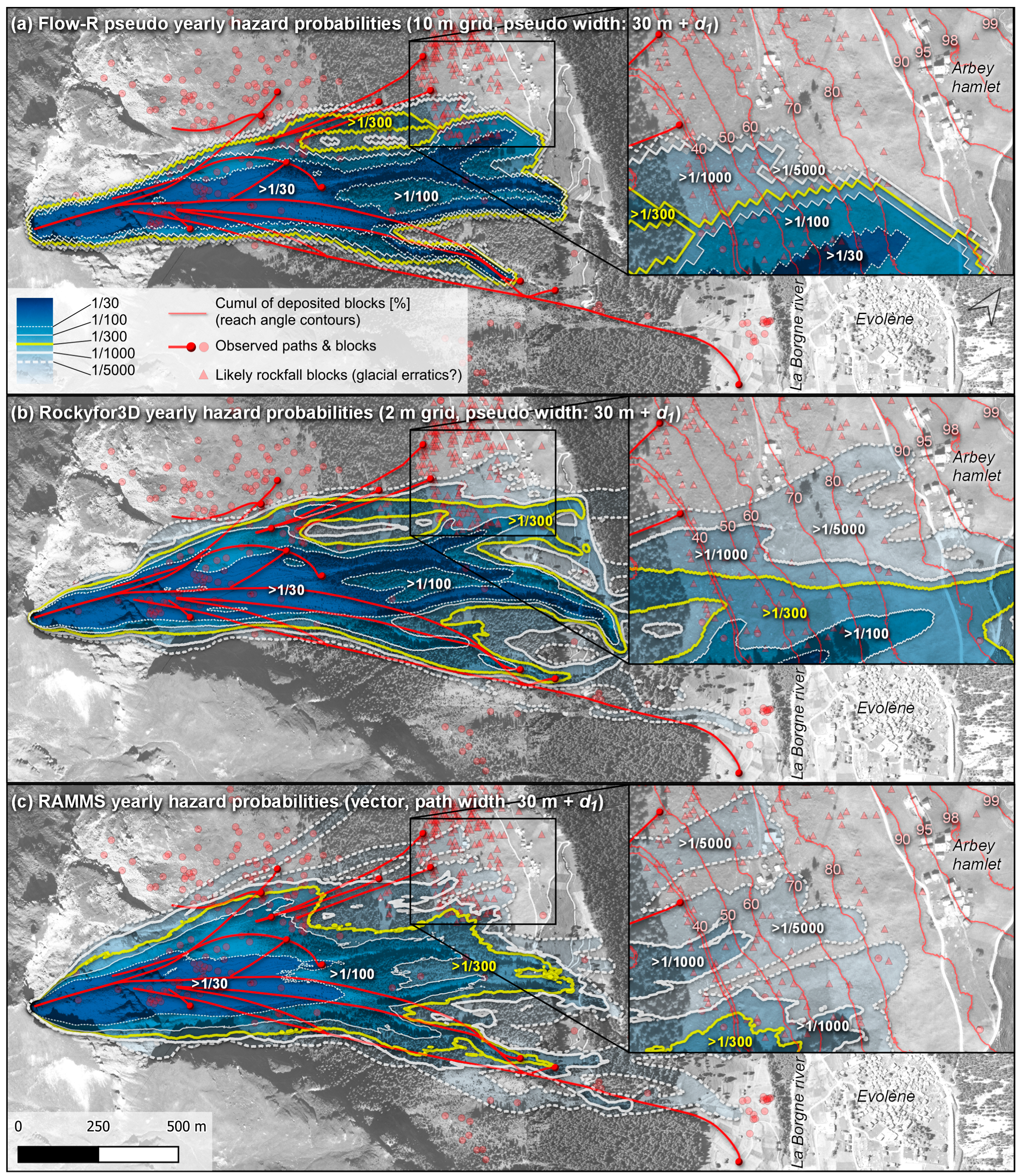
  • Do the simulated paths unrealistically oscillate laterally compared to the observations, potentially leading to unrealistically undertaken paths and erroneous associated reach probabilities (e.g., the yellow vs. red paths in Figure 1a,b)?
  • Do the small sets of simulated paths and their distribution fall close to the observations for similar paths so that the simulations are statistically representative (e.g., the yellow vs. red paths in Figure 1a,c)?
  • Do the vaults or curvature of the simulated freefalling parabola segments and separating distances in between the impacts compare well with the observations so that the bounce heights are realistic for use of the simulation with mitigation design tasks?
  • Do the simulated velocities or related energies compare well with those from the reconstructed trajectories so that intensities based on preset building vulnerabilities can be estimated for land planning zonation tasks, risk assessment studies or mitigation design tasks?
  • Are the simulated velocities, bounce heights and deposited rocks matching with the reconstructed data? In other words, is it possible to obtain all those characteristics at once, or must simulations with different parameter values be performed in parallel for each desired piece of matching information?
Combined with Figure 6, Figure 5 is also designed to qualitatively evaluate if the area covered by the simulations is statistically representative of a high number of simulated paths (and/or a number equivalent to what may be used when delivering projects). For this validation step, the following questions can be explored:
  • Does the simulated envelope cover most of the mapped deposited rocks suspected to come from the same source(s) so that the results could be used for guiding susceptibility/indicative hazard zoning (e.g., the yellow vs. red dotted envelopes in Figure 1a–c)?
  • Would an additional buffer around the simulated paths and/or different parameter values be needed to increase the area covered by the envelope to catch most of the mapped deposited blocks?
  • Are the simulated paths and deposited rocks overly channelized compared to the mapped observations, leading to unrealistic statistics for the reach probabilities (e.g., the yellow vs. red paths and blocks in Figure 1a,b)?
  • Contrarily, are the simulated rocks deposited near mapped deposited ones in proportional numbers so that the simulations are statistically representative for quantitatively guiding hazard land use zonation and risk-assessment-related tasks (e.g., the yellow vs. red paths and blocks in Figure 1a,c)?
  • Are the path widths properly considered to obtain statistically representative reach probabilities from the propagation probabilities (e.g., see the width influence on the reach probabilities in Figure 1d)?
The results of each software are analyzed individually in the following subsections for objectivity. As a reminder, the volumes and energies involved for that site greatly exceed those of the empirical data used for the development of the process-based simulation software used in this comparison (companion publication Noël et al. [1]). It can thus be challenging for the models to reproduce the rockfall events of that site.

3.1. Flow-R 2.0.9 Analysis

Concerning the first scenario with Flow-R (Figure 3a and Figure 4a) reusing the fine-tuned parameters from Michoud et al. [15] in yellow, many observed paths and deposited blocks (in red) are surprisingly not covered by the 2D gridded simulations despite the similarity of the neighboring valleys covered in Michoud et al. [15]. In fact, most observed blocks that deviate toward their left side when looking downslope are not reached by the simulated envelopes of the three scenarios despite using an exponent of 1 for a high lateral diffusion of the flow equivalent to the one from Quinn et al. [52]. Indeed, the maximal induced lateral diffusion of the simulated flow is not high enough to reproduce the rockfall paths observed for this site. However, increasing the diffusivity by using a smaller exponent value outside of its designed range [1 to ∞] (Horton et al. [18]), which goes against the original intended use of the exponent (Holmgren, [51]), would have the adverse effect of lowering the runouts. Indeed, Flow-R is designed to stop the flow locally when its pseudo quantity, which becomes “diluted” with increasing diffusion, is not sufficient for sustaining the flow propagation, i.e., when the local susceptibility falls below a certain threshold (Horton et al. [18]). When experimenting with a smaller exponent, one should thus lower this threshold.
The lack of lateral spreading is also visible for the 15 extracted paths from the random walk that mostly follow the steepest downslope gradient with local sharp turns due to their eight allowed directions toward the neighboring cells in the raster grid (N, NE, E, SE, S, SW, W and NW) (Figure 3a and Figure 5a). The 2D gridded simulated diffuse flows follow the topography instead of reproducing the observed rockfall paths since 2D hydrological runoff models generally follow the steepest path (Volkwein et al. [6]).
The runouts in directions other than the eight neighboring cells are shortened due to an increased number of sharp turns and small oscillating detours via the neighboring cells (Dorren, [14]). As a result of this grid bias, the simulated envelopes from Flow-R barely managed to reach the CONEFALL reach angle contours of the corresponding parameters used (33°, 31° and 25°), even without a pseudo velocity cutoff (Figure 3a, cumulative curves in Figure 4a and Figure 7). When drawing maximum runout limits based on reach angle thresholds with Flow-R, one should interpret its results with caution because this grid bias affects the predictability of the model. Additionally, one should account for such bias by using high pseudo velocity cutoff values and lower reach angles than the desired ones from empirical rockfall databases. For rockfall modeling, lowering the reach angle by approximately two degrees ensures all areas that would be reached without the grid bias are reached (Figure 7c). The reach angle can be precisely adjusted geometrically (Figure 7b) with Equation (5) as follows:
tan φ A d j u s t e d = cos 45 ° 2   tan φ ,
Future versions of the model could improve on this aspect by considering the second and third 16 to 24 cell neighbors, higher resolution grids and recalibrated the susceptibility threshold as a workaround.
Nevertheless, the reachable envelopes from Flow-R are the easiest to read with a clear distinction from one scenario to the others compared to those of the other software (Figure 3). This can help draw susceptibility/indicative hazard limits. The simulated results were also easy to quickly produce thanks to the efficiency of Flow-R. Therefore, for sites where the expected rockfalls are channelized and do not deviate laterally as much, Flow-R can be an option for the estimation of the area susceptible to rockfalls if low reach angle and high pseudo velocity cutoff parameters are used.
In the case of the pseudo velocities (Figure 4), they differ from those of the reconstructed trajectories with their smooth velocity transitions. Indeed, they lack the typical rockfall sawtooth shapes of the reconstructed trajectory velocities. This is due to the 2D gridded geometrical reach angle approach of Flow-R based on diffusive ground water hydrological runoff and debris flow models (Holmgren, [51]; Gamma, [53]). The applied pseudo velocity cutoff of the third scenario in blue is clearly visible in Figure 4a with the horizontal velocity segments at 30 m s−1. When ignoring the lack of sawtooth shapes from Flow-R’s results, the decreasing velocities of the second scenario match well with the last 1000 m of block 2.
With the questionable hypothetical situation where quantitative rockfall hazard zoning would not require complementary process-based rockfall simulations, one should interpret the simulated results from Flow-R with caution if solely used for that purpose (Figure 5a,b and Figure 6a). Indeed, the 15 extracted paths differ greatly from the historical paths (yellow, green, and blue paths vs. red paths in Figure 3a). However, where in reach by the simulations, the susceptibilities from scenario 2 directly outputted by Flow-R are generally higher than the propagation probabilities from Rockyfor3D and RAMMS, which are safe (Figure 5a,c,e). However, this difference disappears once converted to “reach probabilities” as an intermediate step toward hazard zoning (Figure 5b,d,f). Also, this step does not increase the footprint of lower probability areas in that case (Figure 6a) in comparison to the other process-based results (Figure 6b,c).

3.2. Rockyfor3D 5.2.15 Analysis

Concerning the first scenario with Rockyfor3D (Figure 3b), its blue envelope safely manages to catch most historical paths. It is interesting that this first simulated scenario covers all the observed historical paths using the rapid automatic simulation parameters. Indeed, this preliminary result lies on the safe side, while subsequent results can become increasingly less conservative by reducing the safety margins as the knowledge of the site increases is a safe and effective approach. The envelopes of the first and second scenarios also reproduce the curved end of the longest runout in the lower right corner (the blue envelope plus one thin green trajectory envelope from the second scenario). The envelope of the second scenario is reasonably pulled back, using roughness dissipating (damping) parameters close to the observed roughness in the field. The addition by Dorren [65] of such measurable dissipating parameters over the “traditional” dissipating coefficients (RN and RT) from Pfeiffer and Bowen [31] helps improve the objectivity of the rebound model.
When looking at the cumulative profiles with the previously stated simplifying assumption that the mapped blocks share a common origin (Figure 4b), the rapid automatic simulations in blue safely overestimate the runouts by slightly more than one degree beyond a reach angle of 32.5°. This is the closest to the cumulative curves of the mapped blocks in the most critical part from 80% to 100% of the cumulated blocks of the three software programs tested. Above 20% of the cumulated blocks, the second scenario in green succeeds at closely following the curve of the mapped blocks (all n = 449) and of the 11 blocks with mapped paths that converge to a similar source origin. However, it is slightly shifted to the left around the most critical area, marginally underestimating the maximum runouts as a result. Further fine-tuning of the parameters toward obtaining final simulation results for that case should thus focus on finding values in between the first and second scenarios. From the cumulative profiles, it is interesting to note the large effect of adding 0.2 m, 0.5 m, and 1.0 m to the Rg70, Rg20 and Rg10 roughness of the 25–35° slopes of the third scenario in comparison to the second scenario. These are the only differences between the parameters of the two scenarios and seem to significantly affect the runouts of the 11.1 m block (d1).
Concerning the lateral deviations with Rockyfor3D, the simulated trajectories are marginally less channelized than with Flow-R and form curved paths slightly closer to those observed (Figure 3 and Figure 5). Nevertheless, slight lateral oscillation persists due to the probabilistic deviations applied by Rockyfor3D’s rebound model at impact. However, the deviations are not applied during the freefalling phases. Indeed, the simulated blocks pursue their strait parabolic course without being affected by the obstacles they fly over until their next impact. This allows the blocks to resist deviating toward the steepest downslope direction during freefall, reducing the channelization as a result. However, the 15 extracted simulated trajectories are too channelized to reproduce the 13 historical mapped paths at that site.
Drawing the susceptibility/indicative hazard limits would be facilitated by adding a buffer around the 2 m thin simulated paths due to their small footprint limited to the width of the cell size. Alternatively, this could also be done from a quantitative hazard approach as described in Section 2.4 (Figure 6) using conservative simulated runout distances or a reach probability threshold for the susceptibility contours. Indeed, a pseudo buffer of the width of the block combined with the exposed object is added to pass from the propagation probabilities (Figure 5c) to the reach probabilities (Figure 5d). However, the second scenario is overly channelized, and many mapped deposited block fragments would not be covered unless a very low reach or hazard probability were to be chosen in that case. Such very low probabilities can, however, be obtained easily by simulating a high number of trajectories thanks to the high efficiency of Rockyfor3D.
For the process-based translational velocities (Figure 4b), it is possible to recognize typical rockfall sawtooth velocity profiles on the simulated trajectories. Additionally, most of them stay under 43 m s−1 with what strangely looks like an undocumented velocity cutoff. A few points go beyond this velocity, however. Further investigations on the velocity cutoff can be found in Appendix B. While finalizing this manuscript, the authors received confirmation that there is indeed a velocity cutoff implemented in Rockyfor3D and that its description will be added to the transparent description of the model (Dorren, [46]). Despite this strange behavior, the simulated velocities from the first scenario with the rapid automatic simulation parameters oscillate in a sawtooth pattern near the velocities from the reconstructed trajectories. Those from the second scenario with a roughness similar to that observed onsite do not increase sufficiently after 800 m to match with those from block 2.
Similar to Flow-R, Rockyfor3D’s results were quickly produced thanks to the efficiency of the software. This leaves more resources for the important on-field data collection aspect and facilitate the fine-tuning and calibration processes. Rockyfor3D’s process-based results should also be interpreted with caution with the tested version if used for quantitative rockfall hazard zoning of such challenging sites with significant lateral spreading. If Rockyfor3D’s good predictability and objectivity remain valid when applied to sites involving more channelized rockfall paths, Rockyfor3D should be a good option for safe and objective quantitative hazard zoning. With limited historical paths available or limited resources for extensive back analyses from field observations, Rockyfor3D is a good option for susceptibility mapping out of the three tested software programs with its rapid automatic simulation parameters. Indeed, it has a similar efficiency to Flow-R but with simulated behaviors closer to rockfall dynamics. Additionally, based on the simulation results limited by their early calibration stage for this site, Rockyfor3D seems to have a more objective and safer approach related to the prediction of the runout distances compared to the tested version of RAMMS::ROCKFALL analyzed hereunder.

3.3. RAMMS::ROCKFALL 1.6.70 Analysis

For RAMMS’s results, the envelopes obtained are 10× sparser than those from Rockyfor3D due to the lower number of simulated trajectories despite the considerable time spent on this software compared to the others. As with Rockyfor3D, a buffer should be added to increase the width of the rasterized trajectories because of their small footprint limited to the width of the cell size (2 m). Surprisingly, the parameters of the first scenario, which were also previously used for that same rockfall event (Lu et al. [49]), did not produce the expected corresponding runouts (Figure 3c and Figure 4c). Indeed, as shown by the five yellow trajectories, such simulations struggle to go beyond the 37° reach angle contour. Four out of five trajectories did not go further than 350 m from the source, and two stopped at the foot of the cliff. The cumulative curve also shows that nearly 60% of the simulated blocks for the first scenario stopped with reach angles steeper than 42°, considerably underestimating the runout distances (Figure 4c). Similar results were also obtained using parameters corresponding to the terrain materials encountered on the site. Instead, the two other scenarios with more realistic boosted runouts were obtained by setting the material properties to values further away from what the authors would have anticipated at that site or from what is recommended in the manual of RAMMS for large blocks. The Extra-hard material was applied for most of the first 600 m and to set to Hard for most of the rest of the slopes (Figure 2).
In this fine-tuning calibration process, the results with underestimated runouts were first obtained and gradually moved toward realistic runout values while moving away from parameters that were first thought to correspond with the terrain material properties. Such an approach for the runout distances follows the opposite direction than the previous safe approach from Rockyfor3D. Indeed, time resources must be spent during this fine-tuning process to increase the area susceptible to rockfalls toward realistic values. Overlooking this back analysis process from field observations in that case would have the serious consequence of predicting too short runouts and small areas susceptible to rockfalls. The objectivity and predictability of the model thus seems lower than that of Rockyfor3D for the runout distances given that significantly underestimated runouts were obtained when initially using parameters close to the site properties or those used by others for that same site. Further fine-tuning of the parameters toward obtaining final simulation results for that challenging case should use parameters increasing the runout distances, thus moving away from the anticipated values. The software limitation on the block volume to 100 m3 may have played a role in underestimating the runout distances.
This difficulty in simulating longer runout distances with moderately to very flat blocks might also be caused by a known issue related to the rotation stability of the block shapes with RAMMS. Indeed, the block’s rotations are erroneously not stable around their d1 or d3 axes with the current model, as recently highlighted by Leine et al. [66], and thus struggle to reproduce a “wheel-like” behavior such as the one observed for the block fragments of the 2015 event of the Mel de la Niva site (Noël et al. [1]). Knowing this issue, a correction for the future released versions of RAMMS::ROCKFALL is being implemented. Finalizing this manuscript, the authors received a preview given by the SLF of a prototype of the future corrected version of RAMMS. With the prototype, they tested the first scenario applied in the same way as in this manuscript but with a 200 m3 block 2. The results of the preview seem promising both in terms of predictability and performance (processing time). This will of course remain to be confirmed once implemented in a released version of RAMMS. Meanwhile, the block shapes should be used with caution with the tested version of RAMMS::ROCKFALL when applied for similar challenging sites and volumes far from what was used for the development of the model. At present, the results produced with the latest version available (v.1.7.60), released in October 2022, are similar to those produced with version v.1.6.70 and were produced in a similar amount of time (see the simulation results in the dataset from Noël et al. [48]).
Nevertheless, with the boosted runouts of the second and third scenarios in green and blue (Figure 3c), their extracted trajectories and those visible on the envelopes in the background have the most realistic paths of the three software programs tested. Indeed, they are often parallel to the observed historical red paths, they reproduce similar curvature and lateral deviations, and they are not overly channelized. The envelope of the second scenario with the real shape of block 2 shows slightly shorter runouts compared to the third scenario with the simplified ellipsoid shape despite the blocks sharing the same moments of inertia. They are otherwise similar, but these shape simplification tests should be performed once the rotational stability of the model is corrected. With the most realistic paths and a wider lateral spreading of the three software programs, RAMMS’s results are promising for quantitative hazard zoning purposes on such challenging sites once carefully calibrated to reproduce proper runouts. The results of the second scenario, despite their underestimated runouts, show a wider covered area that matches better with the observations (Figure 5 and Figure 6). With the simulated trajectories also being exported in vector format, the proper addition of path width to pass from the propagation probabilities to the reach probabilities is facilitated. For low hazard probabilities, the number of simulated trajectories should however be increased for the hazard contours to stabilize. This is manifested by the irregular contours mostly visible for the 1/1000 and 1/5000 yearly hazard probabilities (Figure 6). From Equation (2) with the frequency used, an exposed object being reached by 1 trajectory out of 1625 would have a yearly hazard probability of 1/5000. So, 1000 simulated trajectories are clearly not sufficient for defining 1/5000 hazard zones quantitatively for the frequency used.
As expected, the process-based simulated velocities (Figure 4c) do not show any cutoff and show the typical rockfall sawtooth profiles. Interestingly, despite being underestimated by approximately half of the reconstructed velocities of block 2 from 900 to 1400 m, the simulated velocities slowly increase, stabilize, and decelerate, as observed for block 2. The simulated freefalling parabolas are in general more vaulted, as indirectly shown by the gentle decrease in velocity at the beginning of most sawtooth profiles followed by a steeper increase in velocity compared to the reconstructed velocities. This also indirectly indicates that the simulated bounce heights would have been overestimated if the velocities did correspond, which is safe. For the final fine-tuned simulations, one must remember in that case to also double the translational energies since only half of the volume of block 2 could be simulated.
Back analyses from field observations are especially important with the tested version of RAMMS because the parameters might have to be fine-tuned far from their anticipated values to produce safe realistic runouts. Many historical paths and/or deposited block fragments should then be mapped for the necessary meticulous time-consuming iterative fine-tuning of the simulation’s parameters. With the most realistic simulated paths of the three software programs tested, RAMMS’s results are promising for quantitative rockfall hazard zoning and related risk assessment tasks if simulated in sufficient numbers and if properly tuned from extensive back analyses. This is in line with the conclusions of Jarsve [67].

4. Benchmark Summary and Recommendations

The tested versions of the three software programs showed their strengths and weaknesses for reproducing such challenging events involving large 200 m3 block fragments, which is far beyond what the models were originally calibrated to. Future versions of the software programs may lead to different conclusions as models improve. Additionally, the comparisons were performed from simulation results taken at early calibration stages and could have been refined to a certain extent. On that topic, adjusting the runout distances is possible with each software program. Rockyfor3D stands out in this case by first quickly predicting safe runout distances close to the cumulative distribution of the observed blocks with its objective rapid automatic parameters. Any user would thus predictably reproduce the same results for this site with this objective set of parameters. Rockyfor3D also manage to reproduce relatively well the observed runout distances from parameters that objectively correspond with the terrain properties of the site. Based on this, it was shown to be a predictable model on the aspect of the runout distances. As for any models, one should reproduce such a comparison approach on other sites to evaluate the extent of its predictability. In certain conditions, its predictability may be impacted by unexpected erroneous ballistic freefall behaviors as those encountered in Appendix B.
The two other software programs produced results that followed the opposite direction than the previous safe approach from Rockyfor3D. For Flow-R, the runouts were always slightly shorter than what was anticipated based on the reach angles used or the first results using parameters for similar sites. This could be easily corrected using Equation (5) with subsequent scenarios thanks to the efficiency of the model, but one must not neglect the per-site calibration aspect from field observations. With RAMMS, the parameters had to be tuned beyond what seems to correspond to the terrain properties of the site to approach the desired runouts, and they should still be tuned further for subsequent scenarios.
However, adjusting the lateral deviation of Rockyfor3D’s simulations through its parameters is not trivial. Therefore, regardless of subsequent fine-tuned simulations, one should not expect the lateral deviations to differ much from those obtained. In this aspect, Flow-R offers more control on its geometrical hydrologic “rockfall” diffusion if one is willing to experiment beyond the intended exponent limits while carefully adjusting the susceptibility threshold. Of the three tested software programs, RAMMS::ROCKFALL, stands out here by better reproducing the lateral deviations objectively associated with the shapes of the blocks. The predictability issues related to its underestimated runout distances with moderately to very flat blocks are likely to be solved once its gyroscopic stability is fixed (Leine et al. [66]).
This comparison of simulation results taken at early calibration stages shows that there is room for improvements of the current software tested. Depending on the requirements of the rockfall hazard stage involved, combining the use of software programs with different behaviors could be a workaround in the meantime as follows:
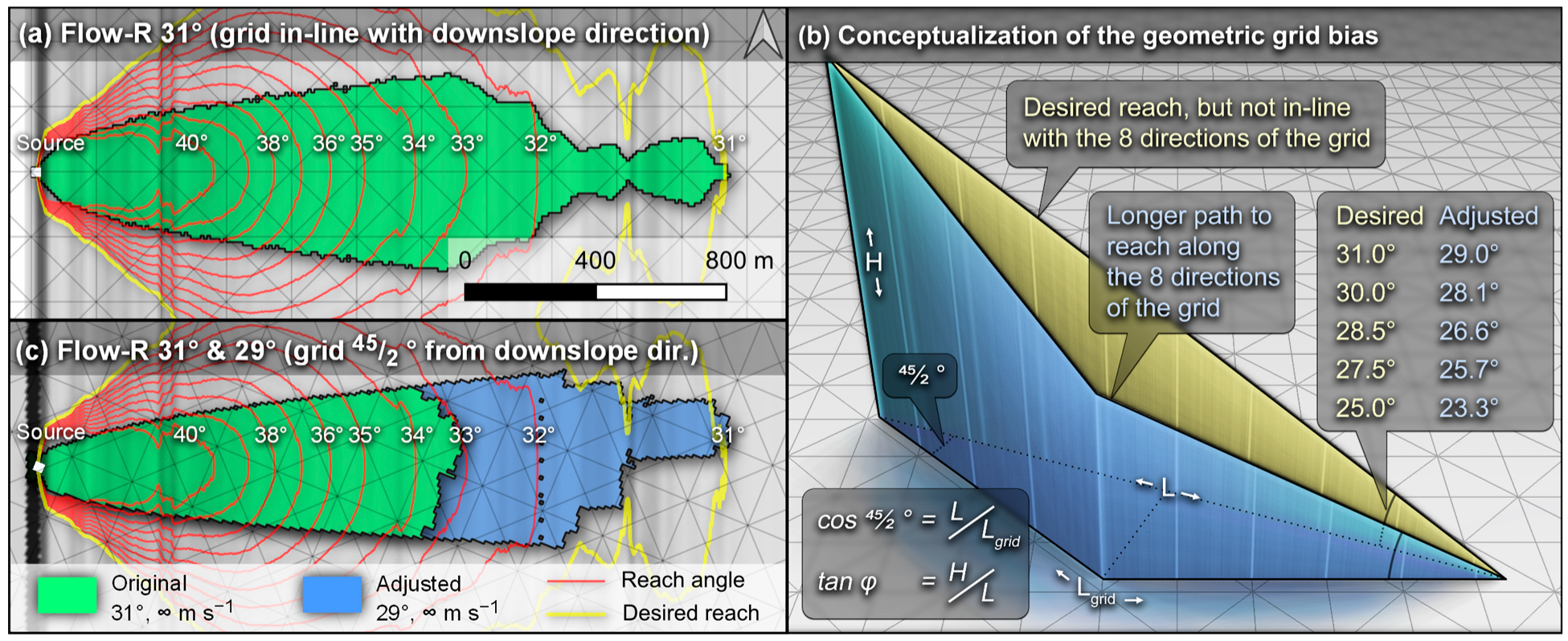
  • One could quickly evaluate the normality/abnormality of a site and preliminary reachable zones by predictably tracing desired reach angle contours from effective and nongrid-biased geometric approaches with, for examples, CONEFALL or QPROTO GIS tools (Jaboyedoff and Labiouse, [17]; Žabota and Kobal, [68]; Scavia et al. [69]; Castelli et al. [70]). Lateral constraints can be roughly estimated from common empirically observed lateral deviations in the literature (Table 2).
  • Then, the use of relatively predictable and time efficient models, such as Rockyfor3D, could be used to estimate the expected runout distances from parameters that can be measured in the field and/or with the conservative parameters with slope thresholds of the rapid automatic simulations.
  • Finally, the realistic lateral extent and energies could be estimated from models, such as RAMMS::ROCKFALL, once its runouts are tuned to match those of the previous conservative/predictable simulations and the onsite observations. One must remember to adjust the energies if the mass of the simulated blocks is constrained by software limitations.
The comparison performed at the challenging site of Mel de la Niva highlighted significant limitations inherent to each model. This reminds us of the inconvenient importance of calibrating the simulations of the current software on a per-site basis from onsite observations, back analyses and back calculations. Even if one may be tempted to trust simulation results blindly to save resources, it is important to be aware that no model is perfect at reproducing reality. Thus, as described in Appendix C, a simple validating back calculation based on rockfall ballistics (e.g., Appendix B) and on field observations should complement simulations. On the simulation software side, providing a back calculation tool would remind and encourage their users to validate their simulation results from field observations and fine-tune the simulations if needed. This is particularly important if the simulations are used for the design of mitigation measures.

5. Conclusions

Simulations from Flow-R 2.0.9, Rockyfor3D 5.2.15 and RAMMS::ROCKFALL 1.6.70 were qualitatively compared to geometrically drawn reach angle contours based on the CONEFALL method and to the mapped rockfall trajectories and deposited block fragments of the Mel de la Niva site from Noël et al. [1]. A focus was placed on evaluating the objectivity, predictability, and sensitivity of the models by comparing simulation results taken at early calibration stages from back analysis for this challenging site. In this way, one can estimate how much the observed runouts may be missed by the simulations when using a reasonable set of parameters for similar sites and how good/poor the predictions may be if overlooking the important back analysis and calibration processes from onsite observations.
The comparison of three scenarios also allowed us to qualitatively evaluate how the models react to changes in their parameters and how far they need to be adjusted beyond what one would have anticipated. The comparison of simulation results taken at early calibration stages showed that there is room for improvements in the current software tested and that combining the use of software with different behaviors could be a workaround in the meantime.
The findings with the current evaluated software also highlight the significant limitation caused by the inconvenient required calibration of the simulations on a per-site basis from onsite observations, back calculations and back analyses. Calibration and validation reasoning steps were given and demonstrated with the presented comparison. Finally, a back calculation tool is provided as Supplementary Material to help and encourage the reader to repeat such comparison and back analyses on other sites.
From a longer-term perspective, this work emphasizes the need for resources to be spent to better understand rockfall dynamics, such as the novel rockfall experiments performed by the SLF and Geobrugg (Caviezel et al. [43,73,74]; Rigenbach et al. [75]; Noël et al. [44]). Hopefully, a better understanding of rockfall phenomena will help improve the objectivity and predictability of rebound models.

Supplementary Materials

The supporting information can be downloaded at https://0-www-mdpi-com.brum.beds.ac.uk/article/10.3390/geosciences13070200/s1. The MATLAB source code of the back calculation tool and the compiled guiding quantitative hazard zoning tool are available “as is”, without warranty of any kind, under the same distribution license as the manuscript (CC BY 4.0), as supplemental material. Further versions can be found within stnParabel rockfall simulation freeware via https://stnparabel.org, (accessed on 21 December 2022) (Noël, [76]) or upon request to the first author.

Author Contributions

Conceptualization, F.N., S.F.N., M.J. and J.L.; methodology, F.N., S.F.N., M.J. and J.L.; software, F.N., S.F.N. and M.J.; validation, F.N., S.F.N., M.J., M.D., A.G., J.L. and B.M.; investigation, F.N., S.F.N., M.J., M.D. and B.M.; resources, F.N., S.F.N., M.J., M.D., J.L. and B.M.; data curation, F.N., S.F.N., M.D. and B.M.; writing—original draft preparation, F.N.; writing—review and editing, F.N., S.F.N., M.J., J.L. and B.M.; visualization, F.N. and S.F.N.; supervision, M.J. and J.L.; project administration, F.N. All authors have read and agreed to the published version of the manuscript.

Funding

This research received no external funding.

Data Availability Statement

The mapped deposited block fragments from the BEG SA Geological Office and the Valais Canton of the 2015 rockfall event are openly available (CC by 4.0) via Noël et al. [48]. The 2019 SfM terrain model and orthophoto of the site are also included. Additionally, the 3D reconstructed trajectories, 2D path segments and blocks are joined to the dataset. The digital elevation model of the site from airborne LiDAR data can be obtained via the swissALTI3D product openly available from ©swisstopo.

Acknowledgments

The authors acknowledge the Valais Canton of Switzerland for providing the valuable video footage and pictures of the 2015 rockfall event. We thank Rambøll Norge AS for the access to the processing resources to perform the RAMMS::ROCKFALL simulations. Finally, the authors would like to acknowledge the anonymous reviewers of the present manuscript.

Conflicts of Interest

The authors declare that they have no conflict of interest.

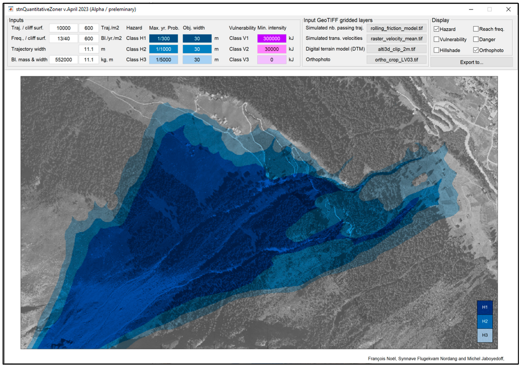
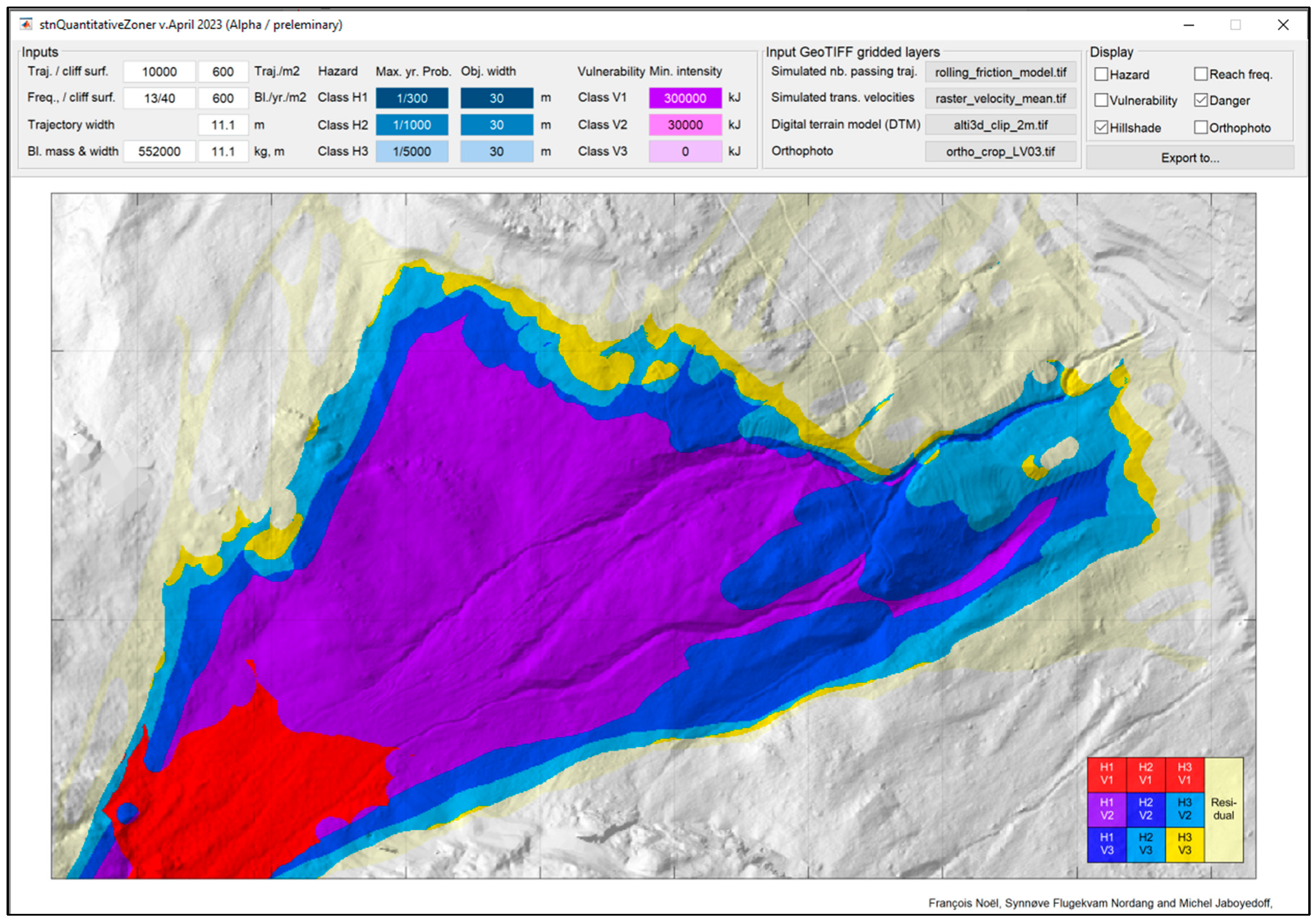
Appendix A. Quantitative Hazard Zoning Tool

As described in the methodology Section 2.4, the simulated results can be expressed in terms of quantified localized reach probability and guiding hazard zones based on (Jaboyedoff et al. [12]). For an exposed object, its local average expected frequency (λobject) of being intercepted by trajectories with exceeding intensities can be evaluated by summing up the number of unique trajectories that intercept the object and exceed the intensity level at which the object is vulnerable. As mentioned in the introduction (Figure 1d), the dimensions of the object and those of the simulated rock fragment must be considered (Jaboyedoff et al. [12]; Corominas et al. [56]; Hantz et al. [11]). This can be done precisely from results in vectorial or point cloud formats with the following steps:
  • Cropping out the trajectory segments with energies/intensities below which the object is not vulnerable. This is done to only keep the “problematic” exceeding segments for a given class. A trajectory with multiple resulting segments should still be counted as one feature.
  • Producing a grid of points spaced to the desired cell size of the end result with an extent that corresponds with the remaining trajectory segments (e.g., with the Create grid tool in QGIS [63]).
  • Converting the points to circular polygons that would represent the hypothetical exposed objects in every location. This can be done by adding a buffer with a radius that corresponds to half of the combined width of the object and blocks.
  • Counting the number of intercepting trajectories in each polygon (e.g., with the Sum line lengths tool in QGIS [63]).
  • Reducing the size of the polygon to only correspond to the dimensions of the object (without the block).
  • Rasterizing the polygons with a priority to the lowest overlaying value (to obtain a zonation valid for the boundaries of the objects) or from the polygon centroids (for a zonation valid for the center of the objects). The obtained raster grid corresponds to the number of reaches.
  • The previous grid can be converted with raster calculations into expected reaching frequencies and hazard probabilities.
  • Contours and/or polygonised contours can be extracted from the hazard probabilities for given hazard thresholds to produce the guiding zonation limits.
A pseudo estimated value can also be estimated from gridded (raster) layers as described at Section 2.4. To facilitate the application of this approach with gridded results from several software programs, we implemented the method in the form of a tool (Figure A1). With gridded layers, it is difficult to precisely exclude trajectory segments with intensities below given thresholds. A conservative approach consists of evaluating the hazard by considering every reaching trajectory without excluding those that do not exceed the intensity thresholds in a first step. The tool uses a moving average window as previously described at Section 2.4 and estimates the pseudo reach frequency and hazard with Equations (3) and (4), respectively. If very high-resolution grids or very large objects are used, the moving window limits its sample size to 100 pixels randomly selected inside the window to speed up the calculation. In contrast with the results presented in this paper, an additional step is added to shift the values to the boundaries of the objects for conveniency.
Figure A1. Interface of the quantitative hazard zoning tool here shown with a SWISSIMAGE orthophoto from ©Swisstopo as base layer and guiding hazard zones for yearly nominal hazard probability thresholds of 1/300, 1/1000 and 1/5000. One can adjust the thresholds and expected frequencies in the inputs to see the results being updated in a matter of seconds (depending on the size of the site and resolution). Gridded results from different simulation software programs can be used if converted to GeoTiff format with corresponding projection and metric units.
Geosciences 13 00200 g0a1
The hazard probabilities and classified zones can also be expressed as danger zones (Figure A2) (i.e., when intensities are combined to the hazard probabilities). This is approximated by excluding the areas with nonexceeding intensities from maximum energies overlay. The energies are calculated from the input translational velocities and mass and are arbitrarily increased by 20% to account for the rotational energy. For an alternative less conservative guiding danger zonation, one can complement the approach by only excluding the intensities from averaged energies (or different output percentiles for example). The comparison of the zonation from those two approaches can give a guiding range where one could be inspired to draw the finalized zonation combined with expert knowledge and field observations.
Figure A2. Interface of the quantitative hazard zoning tool here shown with a hill shade base layer calculated from the swissALTI3D DTM from ©Swisstopo and guiding danger zones for very high intensity thresholds.
Geosciences 13 00200 g0a2
For this site, the output zonation only takes a few seconds to update (for 2 m cell-size). One can thus easily evaluate the effect of different estimated frequencies (from finalized fine-tuned simulations). The same can be done by varying the size of the hypothetical “objects” (e.g., pedestrians, large buildings, etc.) or to quickly evaluate zones, within which mitigation capacities would not be exceeded. The MATLAB-compiled guiding tool is provided in the Supplementary Material.

Appendix B. Rockyfor3D Velocity Cutoff Investigation

Since no velocity cutoff is mentioned in the transparent description of Rockyfor3D’s model (Dorren, [46]), the strange cutoff behavior revealed in Figure 4b deserves a closer look. To investigate, a series of rockfall simulations performed on simplified 3D terrain involving vertical cliffs of different heights are compared to corresponding back-calculated ballistic freefalling parabolas. Different cliff heights are used in order to verify if the behavior can be cause of concern only when high velocities are involved or if it is generalized, i.e., present even when low velocities are involved. First, the simulation methodology is briefly described. The results are then presented and analyzed. Finally, raised questions following the observed behavior of the model are given as a brief conclusion of the investigation.

Appendix B.1. Method

To try to induce conditions where it is likely to observe velocity cutoff, high velocities must be involved. Unfortunately, it is not possible to define custom initial velocities for the simulations other than adding initial fall height (up to 50 m). Therefore, accelerating ramps were rather used to bring the simulated rocks up to having sufficient initial velocities before induced controlled freefall phases from abrupt height drops at the end of the ramps. For that purpose, four artificial 2 m gridded terrain models were created for the investigation (Figure A3). They are described from the rockfall source at their highest point to their lowest elevation in the following sentences. First, they are all composed of a 100 m tall 1:1 (45°) conic ramp where the simulated rocks can accelerate while staying close to the ground. Then, the ramps end abruptly into subvertical cliffs. The cliffs form height drops of 200, 100, 50 and 25 m where the simulated rocks should undergo ballistic freefall. Finally, the terrain models are composed of a flat surface at the base of the cliffs. There, the simulated rocks should decelerate abruptly at their first impact following the long preceding freefall phase. Then, they should rapidly come to a stop after a few short grazing rolling bounces. A Soil type parameter of category 4 was attributed to the terrain, corresponding to a normal damping coefficient parameter (RN) of 0.38 +/− 10%. The velocity damping roughness parameters (Rg70, Rg20 and Rg10), from which the tangential damping coefficient parameter (RT) is derived, were kept to zero to ensure an easy gain in translational velocity. For the following results, the corresponding RT for the expected impact velocities after the long freefall phases goes from 0.50 to 0.75.
Figure A3. Site configurations for the investigation on the strange velocity cutoff experienced with Rockyfor3D. At the bottom end of the conic ramps, the collectors in blue were used to extract the initial conditions before the long freefall phases. From them, the initial heights above the end of the ramp, the velocities and trend angle of the trajectories were used to calculate the expected ballistic freefall parabolas. The location where to expect the parabolas to have their first intercepting impact at the base is highlighted with red circles. Stronger red is used to highlight the average expected first impact location.
Geosciences 13 00200 g0a3
Ten rockfall paths were simulated per terrain model with ellipsoid rocks of dimensions d1-d2-d3 of 2.0-1.8-1.3 m (Figure A3). The sources were placed to the second downslope pixel from the apex of the conic ramps to preserve a required buffer of two pixels from the edges of the grids. An additional fall height of 1 m was added from the source, while the initial velocity was kept untouched.
Collectors covering all pixels of the terrain were used to extract “raw” simulation data. For this, “nets” of zero capacity and height were placed in the form of concentric circles every two meters horizontally from the apex of the conic ramps. As shown in blue in Figure A3, the 49th collectors were used to extract the initial velocities, bounce heights and trend angles of the trajectories at the bottom end of the conic ramps, just before the long controlled freefalling phases due to the cliffs. The individual velocities, heights above the cliff crest and trend angles per simulated trajectory were used as initial conditions to calculate the 40 corresponding expected freefall ballistic parabolas using the common rockfall ballistic equations (e.g., Appendix D). As shown with red circles in Figure A3, the related shortest, average, and maximum horizontal distances from the cliffs/end-of-ramps are then used to highlight where the simulated first impacts are expected to happen. The calculated values from the averaged initial velocities and trend angles are also shown for comparison using the back calculation tool described briefly at Appendix C (Figure A3). With the tool, the slight additional heights of the trajectories above the cliff crests were ignored. This slightly reduces the expected maximum velocities and horizontal distances to the advantage of Rockyfor3D.

Appendix B.2. Results

First, an overview of the simulation results and calculated expected freefalling parabolas is given in 3D in Figure A3, conceptualizing the methodology. The same results are detailed with 2D profiles of the expected ballistic freefall parabolas from the averaged initial conditions and with the simulations seen in 2D from above for the 200, 100, 50 and 25 m cliffs at Figure A4, Figure A5, Figure A6 and Figure A7, respectively.
To the surprise of the authors, the results for the 200 m cliff shown in Figure A4 greatly differ from the expectations, even when anticipating eventual simulated velocity cutoff. Indeed, all simulated first impacts after the long ~200 m vertical height drop significantly miss the zone highlighted in red in Figure A4 where the long freefall parabolas should intercept the flat terrain at the base. Not even the simulated runouts including the following short grazing rolling bounces come close to that zone. Two outlier trajectories manage to have freefall parabolas with longer horizontal travelled distances. Still, their first impacts are only slightly beyond half of the average expected horizontal distance. The maximum simulated velocity (V_max) of 44.71 m s−1, only attained by the two trajectories (Figure A4b), differs with the expected one (vb1) of 68.35 m s−1, calculated from the averaged collected initial conditions without additional height (Figure A4a) and with the maximum expected one of 69.45 m s−1, calculated from the initial conditions of the last collected rock data. In contrast, none of the ten calculated maximum velocities from the collected initial conditions fall under 67.47 m s−1 (second collected rock data), despite one possibly anticipating that high velocities are attained after a 200 m vertical freefall. The end velocities for such rock characteristics should not be influenced much by the drag effect due to the air resistance as shown with the calculated values under parentheses in Figure A4a.
Figure A4. Comparison of the ten simulated trajectories from Rockyfor3D with the expected calculated ballistic freefall parabolas for the 200 m vertical fall. In (a), the back calculation tool is used from the averaged initial conditions, ignoring the additional vertical height above the cliff crest (Ph_vert) of 1.19 m. The initial conditions for the ballistic freefall collected at the bottom end of the conic ramp are shown with the blue table in (b). The expected minimum, average and maximal horizontal ballistic freefall distances are obtained from the ten individually calculated expected ballistic parabolas considering their initial velocity (va), Ph_vert and trend angle (Imp_a). Note that the color scales and velocity values differ in between (a,b).
Geosciences 13 00200 g0a4
The results for the 100 m cliff shown in Figure A5 are similar to those for the 200 m cliff. Again, they greatly differ from the expectations. Indeed, all simulated first impacts after the long ~100 m vertical height drop significantly miss the zone highlighted in red in Figure A5, where all the long freefall parabolas should intercept the flat terrain at the base. As for the previous site, not even the simulated runouts, including the following short grazing rolling bounces, come close to that zone. Again, two trajectories manage to have freefall parabolas with longer horizontal travelled distances. Still, their first impacts are at only two thirds of the average expected horizontal distance. The maximum simulated velocity (V_max) of 42.97 m s−1, only attained by the two trajectories (Figure A5b), differs with the expected one (vb1) of 51.80 m s−1, calculated from the averaged collected initial conditions without additional height (Figure A5a) and with the maximum expected one of 53.12 m s−1, calculated from the initial conditions of the third collected rock data. In contrast, none of the ten calculated maximum velocities from the collected initial conditions fall under 50.90 m s−1 (eighth collected rock data). With shorter freefall distances than for the 200 m cliff, the drag effect due to the air resistance is even smaller, as shown with the calculated values under parentheses in Figure A5a.
Figure A5. Comparison of the ten simulated trajectories from Rockyfor3D with the expected calculated ballistic freefall parabolas for the 100 m vertical fall. In (a), the back calculation tool is used from the averaged initial conditions, ignoring the additional vertical height above the cliff crest (Ph_vert) of 1.56 m. The initial conditions for the ballistic freefall collected at the bottom end of the conic ramp are shown with the blue table in (b). The expected minimum, average and maximal horizontal ballistic freefall distances are obtained from the ten individually calculated expected ballistic parabolas considering their initial velocity (va), Ph_vert and trend angle (Imp_a). Note that the color scales and velocity values differ in between (a,b).
Geosciences 13 00200 g0a5
The results for the 50 m cliff are shown in Figure A6. Compared to the results for the 100 and 200 m cliffs, three simulated trajectories out of ten (30%) manage to reach the zone highlighted in red for the first time, where it is expected that all ten long freefall parabolas intercept the flat terrain at the base. Two of those three trajectories barely reach the shortest expected distance to their first impacts, while the last trajectory reaches the average expected distance. None of the ten simulated trajectories have their first impact at the base beyond the expected average distance for such an impact. This time, one simulated trajectory out of ten (10%) has a maximum simulated velocity (V_max = 41.71 m s−1) that falls in the range of the expected ones calculated from the collected initial conditions. Nine trajectories (90%) remain below the lowest expected maximum velocity of 40.12 m s−1, calculated from the initial conditions of the sixth collected rock data.
Figure A6. Comparison of the ten simulated trajectories from Rockyfor3D with the expected calculated ballistic freefall parabolas for the 50 m vertical fall. In (a), the back calculation tool is used from the averaged initial conditions, ignoring the additional vertical height above the cliff crest (Ph_vert) of 1.38 m. The initial conditions for the ballistic freefall collected at the bottom end of the conic ramp are shown with the blue table in (b). The expected minimum, average and maximal horizontal ballistic freefall distances are obtained from the ten individually calculated expected ballistic parabolas considering their initial velocity (va), Ph_vert and trend angle (Imp_a). Note that the color scales and velocity values differ in between (a,b).
Geosciences 13 00200 g0a6
The results for the 25 m cliff are shown in Figure A7. They are similar to those of the 50 m cliff with three simulated trajectories out of ten (30%) managing to reach the zone highlighted in red in their first impact, where it is expected that all ten long freefall parabolas intercept the flat terrain at the base. Again, two of the three trajectories barely reach the shortest expected distance to their first impacts, while the last trajectory reaches the average expected distance. Still, none of the ten simulated trajectories has their first impact at the base beyond the expected average distance for such an impact. This time, four simulated trajectories out of ten (40%) have maximum simulated velocities (V_max) that fall above the lowest expected one of 33.13 m s−1, calculated from the collected initial conditions of the third rock. Strangely, the overall runouts are longer for that site than for the 200 m cliff if excluding the two outlier trajectories with longer runouts of the later.
Figure A7. Comparison of the ten simulated trajectories from Rockyfor3D with the expected calculated ballistic freefall parabolas for the 25 m vertical fall. In (a), the back calculation tool is used from the averaged initial conditions, ignoring the additional vertical height above the cliff crest (Ph_vert) of 1.77 m. The initial conditions for the ballistic freefall collected at the bottom end of the conic ramp are shown with the blue table in (b). The expected minimum, average and maximal horizontal ballistic freefall distances are obtained from the ten individually calculated expected ballistic parabolas considering their initial velocity (va), Ph_vert and trend angle (Imp_a). Note that the color scales and velocity values differ in between (a,b).
Geosciences 13 00200 g0a7

Appendix B.3. Concluding Remarks

If the simulations were only affected by a velocity cutoff around 43 m s−1, the results for the 25 and 50 m cliff sites should not deviate from expectation since the related expected maximal velocities are below such limit. Discrepancies should be confined to the two sites with the tallest cliffs involving high freefall velocities, while the two other sites should match the expected values. Instead, only 30% of the simulated trajectories at the two smaller cliffs did hit the zone of expected first impacts after the long freefall phases. Moreover, none of the 40 simulated trajectories went beyond the expected average distance for first impact, even for the smaller cliffs. Such results suggest that the strange behavior manifested by the observed velocity cutoff may be a side-effect of a more generalized problem with the implementation of the simulation model in Rockyfor3D 5.2.15. We conclude the investigation by raising a series of related and site-dependent questions:
  • How much of a concern is this for sites involving series of small, stepped cliffs?
  • What about if tall steep cliffs beyond 50 m are involved?
  • Do the rockfalls initiated from such tall cliffs reach proper velocities at the end of their initial freefalling phases, ensuring proper following propagations?
  • Should more than half of the simulated trajectories with shorter runouts be ignored in order to preserve mostly the outlier trajectories when cliffs are present? If so, how can one filter out the “good” trajectories from the “wrong” ones in a practical manner to obtain proper probabilities?

Appendix C. The Importance of Back Calculation

As shown with the results shown in this paper, simulation models often require fine tuning and calibration of their parameters before one can obtain results approaching the observations. This is especially true when models are pushed beyond what they were originally calibrated to. Thus, as also recommended by Labiouse and Heidenreich [77], one must not overlook the important onsite collection of data from previous events. Indeed, to obtain an idea of the possible runout distributions, the main rockfall paths, lateral spreading, involved volumes and rock shapes, data such as the following should be collected:
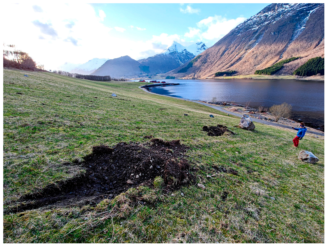
  • Position of the deposited blocks beyond the foot of the scree slopes;
  • Typical dimensions and shapes of those deposited blocks;
  • Position of consecutive impact marks;
  • Intermediate impact marks (e.g., on tree stems);
  • Impact mark characteristics.
Previous onsite rockfall activity and related impact marks can also be highlighted using artificial lighting and shading methods, as shown in Noël et al. [1]. These site observations can be used to reconstruct part of the rockfall’s 2D paths, 3D trajectories and freefalling parabolas. Such back calculation results can then be used for comparing the simulation results as shown previously with the reconstructed and mapped data shown in red in all previous figures.
It is possible to use the CAVR reconstruction method to back calculate the bounce heights and velocities from onsite observations (Noël et al. [44]). The method requires two inputs for the back calculation: (1) the position of the impacts and (2) the freefalling period ( t ). The impact-to-impact distance ( s ) measured at the center of mass of the rocks and related slope ( β s ) can be estimated from the first input after applying an offset function of the rock’s diameter (Figure A8). The freefalling period as the second input can be estimated in four ways depending on the onsite configuration of the observations (calculation details provided in Appendix D):
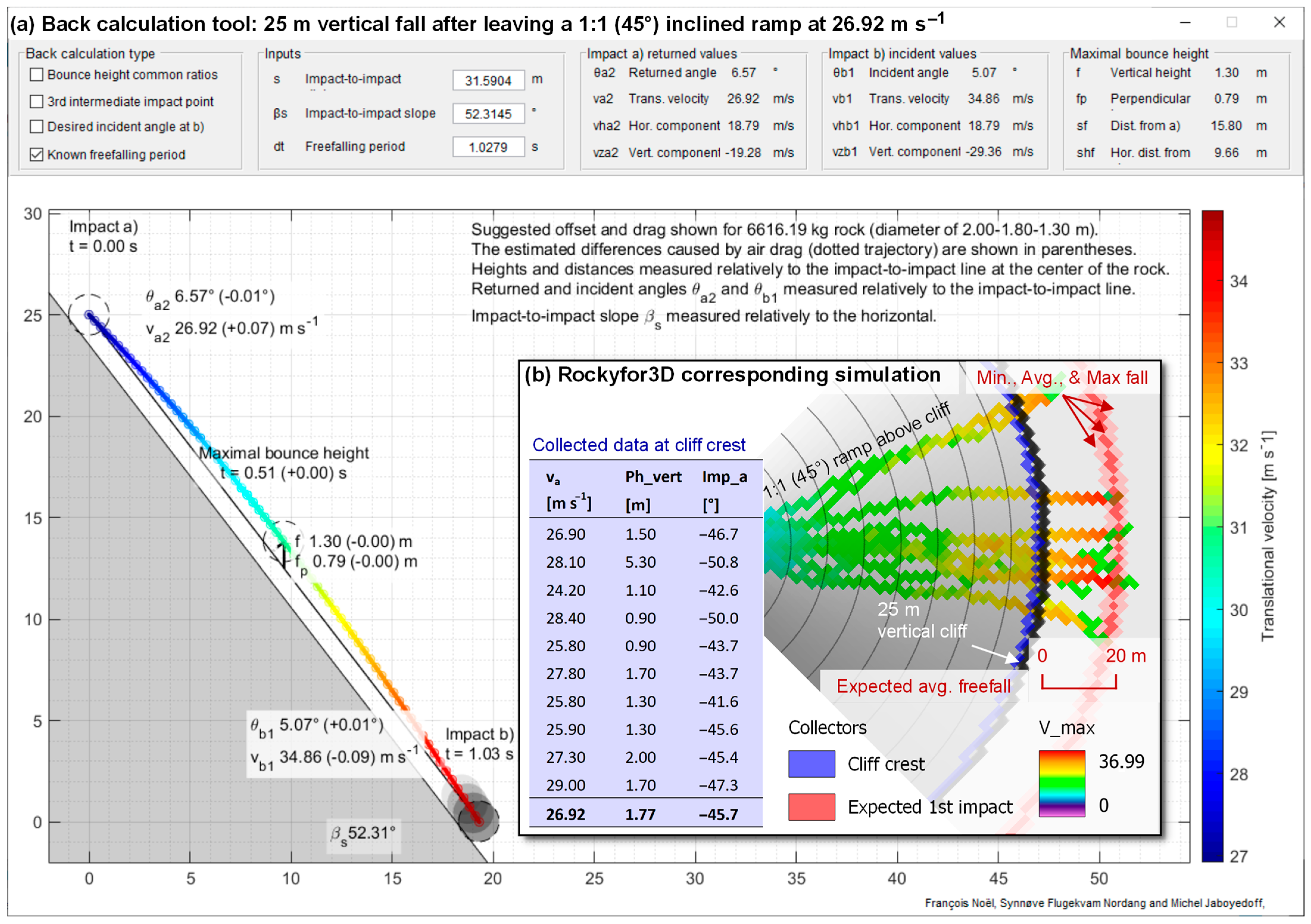
  • As suggested by Volkwein et al. [6], Glover [78] and Gerber [42], it can be defined from a predefined vertical lumped mass bounce height ( f ) from common ratios (e.g., f = s 6 ) (Figure A8). In this case, with g being the vertical acceleration component due to gravity (~−9.81 m s−2), the period is given by Equation (A1) as follows (Volkwein et al. [6]; Glover, [78]; Gerber, [42]):
    t = 8 f g ,
  • The freefalling parabola can be back calculated from an intermediate third impact point (e.g., on a tree stem), assuming no change in velocity or deviation occurs (Paronuzzi, [79]; Volkwein et al., [6]; Wyllie, [41]; Gerber, [42]). With a lumped mass vertical impact height at the third impact ( f 3 ), as shown in Figure A8, and a lumped mass distance from impact (a) ( s 3 ) along the impact-to-impact line, one can find the related period by constraining the common ballistic equations (e.g., Descoeudres, [40]; Wyllie, [41]; Noël et al. [44]) to pass by the three impact points. Once isolated, the related period is given by Equation (A2) as follows:
    t = 2   s 2   f 3 g   s 3   s s 3 ,
  • The freefalling parabola can also be reconstructed from known returned or incident angles (Domaas, [39]; Paronuzzi, [79]; Wyllie, [41]). This is usually done from the incident angle ( θ b ) at the impact (b) relative to the impact-to-impact line (Figure A8) because the entry point of an impact mark is usually much cleaner than the exit point due to the bulged and projected soil that affects the latter (Figure A9). This time, the common ballistic equations must be constrained by the incident trend angle of the incoming trajectory ( tan β s + θ b = d z d x at t = t ). Once isolated, the period in this third case is given by Equation (A3) as follows:
    t = 2   s sin θ b g   cos β s + θ b ,
  • It can finally be measured from video footage (e.g., Descoeudres, [40]; Glover, [78]; Gerber, [42]; Prades-Valls et al. [80]; Noël et al. [44]; Noël et al. [1]), seismic data (e.g., Hibert et al. [81]) or instrumented rocks (Volkwein and Klette, [82]; Gerber, [42]; Caviezel et al. [73]) in unlikely cases, in which past rockfalls were witnessed, filmed, instrumented and/or the site was instrumented.
Figure A8. Back calculation example of a freefalling parabola to show its geometric configuration and related variables.
Geosciences 13 00200 g0a8
Figure A9. Example of an impact scar observed in the field. Note how clearly defined is the entry point of the scar compared to the exit point. As a side note, small rockfalls that occur in fields are likely to be removed by landowners, thus affecting onsite data collection.
Geosciences 13 00200 g0a9
To ease this important back calculation step, some have made calculation tools, precalculated abacuses, or spreadsheets to quickly obtain the desired values from one or many of the previously mentioned configurations (e.g., Paronuzzi, [79]; Volkwein et al. [6]; Dorren et al. [7]; Glover [78]; Gerber, [42]; Kneib et al. [83]). In the same vein, we developed a simple 2D back calculation tool based on the CAVR method (Noël et al. [44]) that brings together these different back calculation configurations. It instantly provides the reconstructed parabola values and produces the related figure (e.g., Figure A8) from two mandatory inputs: (1) the impact-to-impact distance and (2) the impact-to-impact slope. Optional inputs can also be included, depending on the on-side observation’s configuration: (1) the f s ratio, (2) the s 3 and f 3 values of the intermediate 3rd impact, (3) a desired incident angle at impact b, or (4) a desired freefalling period. The MATLAB source code of the tool is provided in the Supplementary Material.

Appendix D. Back Calculation Proofs

The common ballistic equations neglecting air drag (e.g., Domaas, [39]; Descoeudres, [40]; Wyllie, [41]; Volkwein et al. [6]; Gerber, [42] and Noël et al. [44]) used in the CAVR method are as follows in the x–z 2D vertical plane of a rockfall parabola (e.g., Noël et al. [44]):
z t = z a + v z a t + 1 2 g t 2 ,
x t = x a + v x a t = v x t ,
v z t = d z x d t = v z a + g t ,
v x t = d x t d t = v x a = v x b = v x ,
g = d v z d t 9.81   m s 2 ,
g h o r i z o n t a l = d v x d t 0   m s 2 ,
where the position of the center of mass of the rock at impact (a) is x a ,   z a = 0 ,   s   sin β s and its position at impact (b) is x b ,   z b = s   cos β s ,   0 by trigonometry from the impact-to-impact distance ( s ) and related slope ( β s ). The returned vertical velocity component after impact (a) ( v z a ) and the incident vertical velocity component at impact (b) ( v z b ) are given by Equations (A10) and (A11) as follows (Noël et al. [44]):
v z a = z a t b 1 2 g t b ,
v z b = v z a + g t b = z a t b + 1 2 g t b ,
where the time at impact (a) is t a = 0 sec, and the time at impact (b) is t b = t .

Appendix D.1. From Common f/s Ratios

While neglecting air drag (see Appendix A in Noël et al. [44] for more details about the significance of air drag), the position and time of the maximal bounce height ( f ) relative to the impact-to-impact line (Figure A8) are given by Equations (A12)–(A14) as follows (Volkwein et al. [6]; Glover, [78]; Gerber, [42]):
z f = z a 2 + f ,
x f = x b 2 ,
t f = t b 2 ,
Combining Equation (A4) with Equations (A10), (A12) and (A14), one obtains Equations (A15)–(A17) as follows (Volkwein et al. [6]; Glover, [78]; Gerber, [42]):
z f = z a + v z a t f + 1 2 g t f 2 ,
z a 2 + f = z a + z a t b 1 2 g t b t b 2 + 1 2 g t b 2 2 ,
0 = g t b 2 + 8 f ,
By isolating t b in Equation (A17), one finds Equation (A1) for back calculation with a f obtained from common f s ratios as follows (Volkwein et al. [6]; Glover, [78]; Gerber, [42]):
t = 8 f g ,

Appendix D.2. From a 3rd Intermediate Impact Point

Similarly, the position and time of the bounce height ( f 3 ) at a third impact point relative to the impact-to-impact line (Figure A8) are given as a ratio of s by Equations (A18)–(A20) as follows:
z 3 = s s 3 s z a + f 3 ,
x 3 = s 3 s x b ,
t 3 = s 3 s t b ,
As before, by combining Equation (A4) with Equations (A10), (A18) and (A20), one obtains Equations (A21)–(A24) as follows:
z 3 = z a + v z a t 3 + 1 2 g t 3 2 ,
s s 3 s z a + f 3 = z a + z a t b 1 2 g t b s 3 s t b + 1 2 g s 3 s t b 2 ,
s s 3 s s   sin β s + f 3 = s   sin β s + s   sin β s t b 1 2 g t b s 3 s t b + 1 2 g s 3 s t b 2 ,
g   s 3 2 t b 2 = 2 f 3 s 2 + g   s   s 3 t b 2 ,
By isolating t b in Equation (A24), one finds Equation (A2) for back calculation from a third intermediate impact point as follows:
t = 2   s 2   f 3 g   s 3   s s 3 ,

Appendix D.3. From a Desired Incident Angle

The vertical position of the freefalling rock can be expressed as a function of its horizontal position by combining Equations (A4) and (A5) in Equation (A25) as follows:
z x = z a + v z a x t v x + 1 2 g x t v x 2 ,
The plunge ( θ p l u n g e ) of the trajectory can be obtained in any location from the slope gradient of its parabola defined by Equation (A25) in Equation (A26) as follows:
tan θ p l u n g e = d z x d x = v z a v x + g x t v x 2 ,
For a desired incident plunge ( θ p l u n g e _ b = θ b + β s , ) at impact (b), Equations (A5), (A10) and (A26) can be combined into Equations (A27)–(A29) as follows:
tan θ b + β s = v z a v x + g   x b v x 2 ,
tan θ b + β s = z a t b 1 2 g t b x b t b + g   x b x b t b 2 ,
tan θ b + β s = s   sin β s + 1 2 g   t b 2 s   cos β s ,
By isolating t b in Equations (A29), one finds Equations (A3) for back calculation from a desired incident angle at impact b as follows:
t = 2   s sin θ b g   cos β s + θ b ,

References

  1. Noël, F.; Nordang, S.F.; Jaboyedoff, M.; Travelletti, J.; Matasci, B.; Digout, M.; Derron, M.-H.; Caviezel, A.; Hibert, C.; Toe, D.; et al. Highly Energetic Rockfalls: Back Analysis of the 2015 Event from the Mel de La Niva, Switzerland. Landslides 2023, 1–22. [Google Scholar] [CrossRef]
  2. Jones, C.L.; Higgins, J.D.; Andrew, R.D.; Colorado Rockfall Simulation Program. 2000, p. 127. Available online: https://coloradogeologicalsurvey.org/publications/colorado-rockfall-simulation-program/ (accessed on 10 January 2021).
  3. Labiouse, V. Fragmental Rockfall Paths: Comparison of Simulations on Alpine Sites and Experimental Investigation of Boulder Impacts. In Landslides: Evaluation and Stabilization/Glissement de Terrain: Evaluation et Stabilisation, Set of 2 Volumes; CRC Press: Rio de Janeiro, Brazil, 2004; pp. 457–466. [Google Scholar]
  4. Berger, F.; Dorren, L.K.A. Objective Comparison of Rockfall Models Using Real Size Experimental Data. In Disaster Mitigation of Debris Flows, Slope Failures and Landslides; Marui, H., Matjaž, M., Eds.; Universal Academy Press: Tokyo, Japan, 2006; pp. 245–252. [Google Scholar]
  5. Berger, F.; Martin, R.; Auber, B.; Mathy, A. Etude Comparative, En Utilisant l’événement Du 28 Décembre 2008 à Saint Paul de Varces, Du Zonage de l’aléa Chute de Pierre Avec Différents Outils de Simulation Trajectographique et Différentes Matrices d’Aléa; Cemagref UREMGR: Grenoble, France, 2011; p. 226. [Google Scholar]
  6. Volkwein, A.; Schellenberg, K.; Labiouse, V.; Agliardi, F.; Berger, F.; Bourrier, F.; Dorren, L.K.A.; Gerber, W.; Jaboyedoff, M. Rockfall Characterisation and Structural Protection—A Review. Nat. Hazards Earth Syst. Sci. 2011, 11, 2617–2651. [Google Scholar] [CrossRef]
  7. Dorren, L.; Domaas, U.; Kronholm, K.; Labiouse, V. Methods for Predicting Rockfall Trajectories and Run-out Zones. In Rockfall Engineering; John Wiley & Sons, Inc.: Hoboken, NJ, USA, 2013; pp. 143–173. [Google Scholar]
  8. Valagussa, A.; Crosta, G.B.; Frattini, P.; Zenoni, S.; Massey, C. Rockfall Runout Simulation Fine-Tuning in Christchurch, New Zealand. In Engineering Geology for Society and Territory—Volume 2; Lollino, G., Giordan, D., Crosta, G.B., Corominas, J., Azzam, R., Wasowski, J., Sciarra, N., Eds.; Springer International Publishing: Cham, Switzerland, 2015; Volume 2, pp. 1913–1917. ISBN 978-3-319-09056-6. [Google Scholar]
  9. Bourrier, F.; Toe, D.; Garcia, B.; Baroth, J.; Lambert, S. Experimental Investigations on Complex Block Propagation for the Assessment of Propagation Models Quality. Landslides 2021, 18, 639–654. [Google Scholar] [CrossRef]
  10. Noël, F.; Cloutier, C.; Jaboyedoff, M.; Locat, J. Impact-Detection Algorithm That Uses Point Clouds as Topographic Inputs for 3D Rockfall Simulations. Geosciences 2021, 11, 188. [Google Scholar] [CrossRef]
  11. Hantz, D.; Corominas, J.; Crosta, G.B.; Jaboyedoff, M. Definitions and Concepts for Quantitative Rockfall Hazard and Risk Analysis. Geosciences 2021, 11, 158. [Google Scholar] [CrossRef]
  12. Jaboyedoff, M.; Dudt, J.P.; Labiouse, V. An Attempt to Refine Rockfall Hazard Zoning Based on the Kinetic Energy, Frequency and Fragmentation Degree. Nat. Hazards Earth Syst. Sci. 2005, 5, 621–632. [Google Scholar] [CrossRef]
  13. Loup, B.; Dorren, L.K.A. Utilisation de Modèles Pour l’Évaluation des Dangers de Chute de Pierres-Fiche d’Information; Office fédéral de l’Environnement (OFEV): Bern, Switzerland, 2022.
  14. Dorren, L.K.A. A Review of Rockfall Mechanics and Modelling Approaches. Prog. Phys. Geogr. Earth Environ. 2003, 27, 69–87. [Google Scholar] [CrossRef]
  15. Michoud, C.; Derron, M.-H.; Horton, P.; Jaboyedoff, M.; Baillifard, F.-J.; Loye, A.; Nicolet, P.; Pedrazzini, A.; Queyrel, A. Rockfall Hazard and Risk Assessments along Roads at a Regional Scale: Example in Swiss Alps. Nat. Hazards Earth Syst. Sci. 2012, 12, 615–629. [Google Scholar] [CrossRef]
  16. Domaas, U. Geometrical Methods of Calculating Rockfall Range; Norwegian Geotechnical Institute: Oslo, Norway, 1994; p. 33. [Google Scholar]
  17. Jaboyedoff, M.; Labiouse, V. Technical Note: Preliminary Estimation of Rockfall Runout Zones. Nat. Hazards Earth Syst. Sci. 2011, 11, 819–828. [Google Scholar] [CrossRef]
  18. Horton, P.; Jaboyedoff, M.; Rudaz, B.; Zimmermann, M. Flow-R, a Model for Susceptibility Mapping of Debris Flows and Other Gravitational Hazards at a Regional Scale. Nat. Hazards Earth Syst. Sci. 2013, 13, 869–885. [Google Scholar] [CrossRef]
  19. ONR 24810 Technical Protection against Rockfall-Terms and Definitions, Effects of Actions, Design, Monitoring and Maintenance. 2013. Available online: https://shop.austrian-standards.at/action/en/public/details/462231/ONR_24810_2013_01_15 (accessed on 6 August 2022).
  20. OFEV. Protection Contre Les Dangers Dus Aux Mouvements de Terrain. Aide à l’exécution Concernant La Gestion Des Dangers Dus Aux Glissements de Terrain, Aux Chutes de Pierres et Aux Coulées de Boue; Office Fédéral de l’Environnement: Bern, Switzerland, 2016; p. 100.
  21. Mölk, M.; Rieder, B. Rockfall Hazard Zones in Austria. Experience, Problems and Solutions in the Development of a Standardised Procedure. Geomech. Tunn. 2017, 10, 24–33. [Google Scholar] [CrossRef]
  22. DiBK. Regulations on technical requirements for construction works (TEK17) with guidance; Direktoratet for Byggkvalitet [Norwegian Building Authority]: Oslo, Norway, 2017; pp. 1–404.
  23. NVE. Veileder-Sikkerhet Mot Skred i Bratt Terreng-Kartlegging Av Skredfare i Reguleringsplan Og Byggesak; Norwegian Water Resources and Energy Directorate (NVE): Oslo, Norway, 2020.
  24. Frattini, P.; Crosta, G.B.; Carrara, A.; Agliardi, F. Assessment of Rockfall Susceptibility by Integrating Statistical and Physically-Based Approaches. Geomorphology 2008, 94, 419–437. [Google Scholar] [CrossRef]
  25. Noël, F. Cartographie Semi-Automatisée Des Chutes de Pierres Le Long d’infrastructures Linéaires. Master’s Thesis, Université Laval, Québec, QC, Canada, 2016. [Google Scholar]
  26. Dupire, S.; Toe, D.; Barré, J.-B.; Bourrier, F.; Berger, F. Harmonized Mapping of Forests with a Protection Function against Rockfalls over European Alpine Countries. Appl. Geogr. 2020, 120, 102221. [Google Scholar] [CrossRef]
  27. Kalsnes, B.; Solheim, A.; Sverdrup-Thygeson, K.; Dingsør-Dehlin, F.; Wasrud, J.; Indrevær, K.; Bergbjørn, K. Flom Og Skred-Sikringsbehov for Eksisterende Bebyggelse (FOSS): Beskrivelse Av Metodikk Og Resultater; NVE: Oslo, Norway, 2021; p. 89.
  28. Alvioli, M.; Santangelo, M.; Fiorucci, F.; Cardinali, M.; Marchesini, I.; Reichenbach, P.; Rossi, M.; Guzzetti, F.; Peruccacci, S. Rockfall Susceptibility and Network-Ranked Susceptibility along the Italian Railway. Eng. Geol. 2021, 293, 106301. [Google Scholar] [CrossRef]
  29. Alvioli, M.; De Matteo, A.; Castaldo, R.; Tizzani, P.; Reichenbach, P. Three-dimensional simulations of rockfalls in Ischia, Southern Italy, and preliminary susceptibility zonation. Geomat. Nat. Hazards Risk 2022, 13, 2712–2736. [Google Scholar] [CrossRef]
  30. Dorren, L.; Schaller, C.; Erbach, A.; Moos, C. Automated Delimitation of Rockfall Hazard Indication Zones Using High-Resolution Trajectory Modelling at Regional Scale. Geosciences 2023, 13, 182. [Google Scholar] [CrossRef]
  31. Pfeiffer, T.J.; Bowen, T.D. Computer Simulation of Rockfalls. Environ. Eng. Geosci. 1989, xxvi, 135–146. [Google Scholar] [CrossRef]
  32. Evans, S.G.; Hungr, O. The Assessment of Rockfall Hazard at the Base of Talus Slopes. Can. Geotech. J. 1993, 30, 620–636. [Google Scholar] [CrossRef]
  33. Raetzo, H.; Lateltin, O.; Bollinger, D.; Tripet, J.P. Hazard Assessment in Switzerland-Codes of Practice for Mass Movements. Bull. Eng. Geol. Environ. 2002, 61, 263–268. [Google Scholar] [CrossRef]
  34. Lambert, S.; Bourrier, F. Design of Rockfall Protection Embankments: A Review. Eng. Geol. 2013, 154, 77–88. [Google Scholar] [CrossRef]
  35. Lambert, S.; Toe, D.; Mentani, A.; Bourrier, F. A Meta-Model-Based Procedure for Quantifying the On-Site Efficiency of Rockfall Barriers. Rock Mech. Rock Eng. 2021, 54, 487–500. [Google Scholar] [CrossRef]
  36. Berger, F.; Corominas, J.; Lopez Carreras, C.; Brauner, M.; Kienholz, H.; Bartelt, P. Rock for Project-Efficiency of the Protective Function of Mountain Forest against Rockfall: Elements for Strategic Planning Tools Dedicated to a Forest Sustainable Mitigation against Rockfall; Centre National du Machinisme Agricole (CEMAGREF): Grenoble, France, 2004; p. 229. [Google Scholar]
  37. Garcia, B. Analyse Des Mécanismes d’Interaction Entre Un Bloc Rocheux et Un Versant de Propagation: Application à l’Ingénierie; Université Grenoble Alpes: Saint-Martin-d’Hères, France, 2019. [Google Scholar]
  38. C2ROP, A. participants of A. 3. 1 Benchmark Des Approches d’analyse Trajectographique Par Analyse Comparative de Simulations Prédictives et d’essais de Terrain. Rev. Fr. Géotech. 2020, 6, 12. [Google Scholar] [CrossRef]
  39. Domaas, U. Natural Rockfalls-Descriptions and Calculations; Norwegian Geotechnical Institute (NGI): Oslo, Norway, 1995. [Google Scholar]
  40. Descoeudres, F. Aspects Géomécaniques Des Instabilités de Falaises Rocheuses et Des Chutes de Blocs. Publ. Société Suisse Méc. Sols Roches 1997, 135, 3–11. [Google Scholar]
  41. Wyllie, D.C. Rock Fall Engineering: Development and Calibration of an Improved Model for Analysis of Rock Fall Hazards on Highways and Railways; The University of British Columbia: Vancouver, BC, Canada, 2014. [Google Scholar]
  42. Gerber, W. Naturgefahr Steinschlag-Erfahrungen Und Erkenntnisse; Eidg. Forschungsanstalt für Wald, Schnee und Landschaft WSL: Birmensdorf, Switzerland, 2019; Volume 74, p. 149. [Google Scholar]
  43. Caviezel, A.; Demmel, S.E.; Ringenbach, A.; Bühler, Y.; Lu, G.; Christen, M.; Dinneen, C.E.; Eberhard, L.A.; von Rickenbach, D.; Bartelt, P. Reconstruction of Four-Dimensional Rockfall Trajectories Using Remote Sensing and Rock-Based Accelerometers and Gyroscopes. Earth Surf. Dyn. 2019, 7, 199–210. [Google Scholar] [CrossRef]
  44. Noël, F.; Jaboyedoff, M.; Caviezel, A.; Hibert, C.; Bourrier, F.; Malet, J.-P. Rockfall Trajectory Reconstruction: A Flexible Method Utilizing Video Footage and High-Resolution Terrain Models. Earth Surf. Dyn. 2022, 10, 1141–1164. [Google Scholar] [CrossRef]
  45. Lambert, S.; Bourrier, F.; Toe, D. Improving Three-Dimensional Rockfall Trajectory Simulation Codes for Assessing the Efficiency of Protective Embankments. Int. J. Rock Mech. Min. Sci. 2013, 60, 26–36. [Google Scholar] [CrossRef]
  46. Dorren, L. Rockyfor3D (v5.2) Revealed-Transparent Description of the Complete 3D Rockfall Model; ecorisQ: Geneva, Switzerland, 2015; p. 31. [Google Scholar]
  47. Leine, R.I.; Schweizer, A.; Christen, M.; Glover, J.; Bartelt, P.; Gerber, W. Simulation of Rockfall Trajectories with Consideration of Rock Shape. Multibody Syst. Dyn. 2014, 32, 241–271. [Google Scholar] [CrossRef]
  48. Noël, F.; Nordang, S.F.; Jaboyedoff, M.; Travelletti, J.; Matasci, B.; Digout, M.; Vogel, A.; Mayoraz, R. Highly Energetic Rockfalls: Dataset of the 2015 Event from the Mel de La Niva, Switzerland. Zenodo 2023. [Google Scholar] [CrossRef]
  49. Lu, G.; Caviezel, A.; Christen, M.; Bühler, Y.; Bartelt, P. Modelling Rockfall Dynamics Using (Convex) Non-Smooth Mechanics. In Numerical Methods in Geotechnical Engineering IX; CRC Press: London, England, 2018; pp. 575–583. ISBN 978-1-138-33198-3. [Google Scholar]
  50. Corominas, J. The Angle of Reach as a Mobility Index for Small and Large Landslides. Can. Geotech. J. 1996, 33, 260–271. [Google Scholar] [CrossRef]
  51. Holmgren, P. Multiple Flow Direction Algorithms for Runoff Modelling in Grid Based Elevation Models: An Empirical Evaluation. Hydrol. Process. 1994, 8, 327–334. [Google Scholar] [CrossRef]
  52. Quinn, P.; Beven, K.; Chevallier, P.; Planchon, O. The Prediction of Hillslope Flow Paths for Distributed Hydrological Modelling Using Digital Terrain Models. Hydrol. Process. 1991, 5, 59–79. [Google Scholar] [CrossRef]
  53. Gamma, P. Dfwalk-Ein Murgang Simulationsprogramm Zur Gefahrenzonierung. 2000. Available online: https://worldcat.org/title/80872939 (accessed on 23 February 2021).
  54. Cloutier, C.; Locat, J.; Mayers, M.; Noël, F.; Jacob, C.; Dorval, P.; Bossé, F.; Gionet, P.; Jaboyedoff, M. An Integrated Management Tool for Rockfall Evaluation along Transportation Corridors: Description and Objectives of the ParaChute Research Project. In Proceedings of the Conférence Canadienne de Géotechnique GEOQuébec 2015, Québec, QC, Canada, 20–23 September 2015; p. 7. [Google Scholar]
  55. Cloutier, C.; Turmel, D.; Mayers, M.; Noël, F.; Locat, J. Projet ParaChute: Développement d’un Outil de Gestion Intégrée Des Chutes de Pierres Le Long d’infrastructures Linéaires; Université Laval: Québec, QC, Canada, 2017; p. 213. [Google Scholar]
  56. Corominas, J.; Copons, R.; Moya, J.; Vilaplana, J.M.; Altimir, J.; Amigó, J. Quantitative Assessment of the Residual Risk in a Rockfall Protected Area. Landslides 2005, 2, 343–357. [Google Scholar] [CrossRef]
  57. Agliardi, F.; Crosta, G.B. High Resolution Three-Dimensional Numerical Modelling of Rockfalls. Int. J. Rock Mech. Min. Sci. 2003, 40, 455–471. [Google Scholar] [CrossRef]
  58. Crosta, G.B.; Agliardi, F. Parametric Evaluation of 3D Dispersion of Rockfall Trajectories. Nat. Hazards Earth Syst. Sci. 2004, 4, 583–598. [Google Scholar] [CrossRef]
  59. EG4 Risk HY-STONE. Available online: http://www.eg4risk.com/en/home-page/ (accessed on 24 April 2022).
  60. Matas, G.; Lantada, N.; Corominas, J.; Gili, J.A.; Ruiz-Carulla, R.; Prades, A. RockGIS: A GIS-Based Model for the Analysis of Fragmentation in Rockfalls. Landslides 2017, 14, 1565–1578. [Google Scholar] [CrossRef]
  61. Abbruzzese, J.M.; Labiouse, V. New Cadanav Methodology for Rock Fall Hazard Zoning Based on 3D Trajectory Modelling. Geosciences 2020, 10, 434. [Google Scholar] [CrossRef]
  62. Lan, H.; Derek Martin, C.; Lim, C.H. RockFall Analyst: A GIS Extension for Three-Dimensional and Spatially Distributed Rockfall Hazard Modeling. Comput. Geosci. 2007, 33, 262–279. [Google Scholar] [CrossRef]
  63. QGIS. Development Team QGIS Geographic Information System. 2023. Available online: https://qgis.org/en/site/ (accessed on 5 January 2023).
  64. MEZAP Group. MEZAP Technical Guide. Caractérisation de l’aléa Rocheux Dans Le Cadre d’un Plan de Prévention Des Risques Naturels (PPRn) Ou d’un Porter à Connaissance (PAC); BRGM: Orléans, France, 2021. [Google Scholar]
  65. Dorren, L.K.A. Rockfall and Protection Forests–Models, Experiments and Reality; Universität für Bodenkultur: Bern, Switzerland, 2008. [Google Scholar]
  66. Leine, R.I.; Capobianco, G.; Bartelt, P.; Christen, M.; Caviezel, A. Stability of Rigid Body Motion through an Extended Intermediate Axis Theorem: Application to Rockfall Simulation. Multibody Syst. Dyn. 2021, 52, 431–455. [Google Scholar] [CrossRef]
  67. Jarsve, K.T. Uncertainties of Simulating Rockfalls and Debris Flows Using RAMMS; University of Oslo: Oslo, Norway, 2018. [Google Scholar]
  68. Žabota, B.; Kobal, M. A New Methodology for Mapping Past Rockfall Events: From Mobile Crowdsourcing to Rockfall Simulation Validation. ISPRS Int. J. Geo-Inf. 2020, 9, 514. [Google Scholar] [CrossRef]
  69. Scavia, C.; Barbero, M.; Castelli, M.; Marchelli, M.; Peila, D.; Torsello, G.; Vallero, G. Evaluating Rockfall Risk: Some Critical Aspects. Geosciences 2020, 10, 98. [Google Scholar] [CrossRef]
  70. Castelli, M.; Torsello, G.; Vallero, G. Preliminary Modeling of Rockfall Runout: Definition of the Input Parameters for the QGIS Plugin QPROTO. Geosciences 2021, 11, 88. [Google Scholar] [CrossRef]
  71. Ushiro, T.; Tsutsui, H. Movement of Rockfall and a Study on Its Prediction. In Proceedings of the International Symposium on Geotechnical & Environmental Challenges in Mountainous Terrain, Kathmandu, Nepal, 6–7 November 2001; pp. 366–375. [Google Scholar]
  72. Dorren, L.K.A.; Berger, F. Stem Breakage of Trees and Energy Dissipation during Rockfall Impacts. Tree Physiol. 2006, 26, 63–71. [Google Scholar] [CrossRef] [PubMed]
  73. Caviezel, A.; Ringenbach, A.; Demmel, S.E.; Dinneen, C.E.; Krebs, N.; Bühler, Y.; Christen, M.; Meyrat, G.; Stoffel, A.; Hafner, E.; et al. The Relevance of Rock Shape over Mass—Implications for Rockfall Hazard Assessments. Nat. Commun. 2021, 12, 5546. [Google Scholar] [CrossRef] [PubMed]
  74. Caviezel, A.; Demmel, S.E.; Bühler, Y.; Ringenbach, A.; Christen, M.; Bartelt, P. Induced Rockfall Dataset #2 (Chant Sura Experimental Campaign), Flüelapass, Grisons, Switzerland. EnviDat 2020. [Google Scholar] [CrossRef]
  75. Ringenbach, A.; Bebi, P.; Bartelt, P.; Rigling, A.; Christen, M.; Bühler, Y.; Stoffel, A.; Caviezel, A. Modeling Deadwood for Rockfall Mitigation Assessments in Windthrow Areas. Earth Surf. Dyn. 2022, 10, 1303–1319. [Google Scholar] [CrossRef]
  76. Noël, F. StnParabel. Available online: https://stnparabel.org/ (accessed on 28 April 2022).
  77. Labiouse, V.; Heidenreich, B. Half-Scale Experimental Study of Rockfall Impacts on Sandy Slopes. Nat. Hazards Earth Syst. Sci. 2009, 9, 1981–1993. [Google Scholar] [CrossRef]
  78. Glover, J.M.H. Rock-Shape and Its Role in Rockfall Dynamics; Durham University: Durham, UK, 2015. [Google Scholar]
  79. Paronuzzi, P. Rockfall-Induced Block Propagation on a Soil Slope, Northern Italy. Environ. Geol. 2009, 58, 1451–1466. [Google Scholar] [CrossRef]
  80. Prades-Valls, A.; Corominas, J.; Lantada, N.; Matas, G.; Núñez-Andrés, M.A. Capturing Rockfall Kinematic and Fragmentation Parameters Using High-Speed Camera System. Eng. Geol. 2022, 302, 106629. [Google Scholar] [CrossRef]
  81. Hibert, C.; Noël, F.; Toe, D.; Talib, M.; Desrues, M.; Wyser, E.; Brenguier, O.; Bourrier, F.; Toussaint, R.; Malet, J.-P.; et al. Machine Learning Prediction of the Mass and the Velocity of Controlled Single-Block Rockfalls from the Seismic Waves They Generate. Earth Surf. Dyn. 2022. Available online: https://0-doi-org.brum.beds.ac.uk/10.5194/egusphere-2022-522 (accessed on 23 September 2022). [CrossRef]
  82. Volkwein, A.; Klette, J. Semi-Automatic Determination of Rockfall Trajectories. Sensors 2014, 14, 18187–18210. [Google Scholar] [CrossRef]
  83. Kneib, F.; Bourrier, F.; Toe, D.; Berger, F. PlatRock. Available online: http://platrock.org/ (accessed on 3 May 2023).
Figure 1. Conceptualization of the validation process when comparing simulation results (yellow) to field observations (red). The resulting related reach probabilities from the simulations are expressed with shades of blue. For definition, the propagation probabilities are given by the number of simulated passing trajectories at a given location divided by the total number of simulated trajectories from a single source. The same is done to obtain the reach probabilities not related to time but with larger trajectory footprints that combine the diameter of the rocks to the exposed object’s width (and potentially the intensities). The hazard probabilities are obtained for a given reference period (e.g., yearly) by combining the frequency of block fragments expected for the site during the given reference period with the reach probability (for more details and definitions, see Jaboyedoff et al. [12] and Hantz et al. [11]).
Geosciences 13 00200 g001
Figure 2. The Mel de la Niva Mountain site described in Noël et al. [1] shown with the mapped blocks and reconstructed rockfall paths in red in (a). The categorized terrain slopes are colored based on the thresholds used for defining the terrain properties (Table 1). Examples of the most encountered terrain types are given in (bd) and are located as references in (a).
Geosciences 13 00200 g002
Figure 3. The simulated paths and envelopes for the three scenarios from the three software programs, shown in yellow, green and blue, are compared to the mapped historical rockfall paths and block fragments shown in red. The five paths randomly selected from each scenario provide insight into the simulated propagation probability by roughly representing the paths that are the most likely to be followed by each simulation model. The colored backgrounds correspond to the envelope given by all simulated paths per scenario. Red contours every 1° corresponding to the reach angles from the source based on the CONEFALL method (Jaboyedoff and Labiouse, [17]) are overlaid as a visual guide.
Geosciences 13 00200 g003
Figure 4. Translational velocity profiles of the three sets of five simulated paths/trajectories for each tested software compared with the two reconstructed trajectories of the 2015 rockfall event from Mel de la Niva as observations. The runout distances of the simulated blocks are compared with the mapped block fragments in terms of cumulative curves of the number of deposited blocks in relation to their reach angles (simplifying by assuming a common source). As a reminder, the runout distances usually increase as their reach angles decrease; this is why the inverted reach angle axes preserve the homogeneity across the paper with rockfalls moving from left to right.
Geosciences 13 00200 g004
Figure 5. Distinction between the simulated results of the second scenarios between the propagation probabilities (on the left) and the reach probabilities (on the right) for exposed objects with a width of 30 m perpendicular to the rockfall paths, as conceptualized in Figure 1d. In the case of a single source, the propagation probabilities are given by the number of simulated passing paths at a given location divided by the total number of simulated paths. The same is done to obtain the reach probabilities but with larger path footprints that combine the diameter of the rocks to the exposed object’s width.
Geosciences 13 00200 g005
Figure 6. Yearly hazard probabilities based on the results of the second scenario for a frequency of 13 bl./40 yr. The probability of 1/300, which is close to the return period used in Switzerland to delimitate the buildable areas for residences when high energies are involved, is shown in yellow. The corresponding threshold used in Norway is set for a yearly probability of 1/1000 (see TEK17 from DiBK, [22]) or at a minimum of 1/10,000 in France (MEZAP group, [64]), for example. Base layer SWISSIMAGE orthophoto from ©Swisstopo.
Geosciences 13 00200 g006
Figure 7. Flow-R simulations as in scenario 2 (31°, ∞ m s−1) on identical extruded 2D profiles of the Mel de la Niva site in (a,c). They highlight the differences induced by the biased gridded approach when the elevation grid is not in line with the flow path direction. In (a), the runout distance is maximum, as its direction toward the downslope direction is in line with the elevation grid. In (c), the runout distance is minimum as the grid orientation mismatches the flow path direction by half of 45°. Red contours every 1° corresponding to the reach angles from the source based on the CONEFALL method (Jaboyedoff and Labiouse, [17]) are overlaid as a visual guide. The geometric representation of the grid bias is shown in (b) with recommended adjusted reach angle values from Equation (5) to circumvent the bias.
Geosciences 13 00200 g007
Table 1. Parameters used for the three scenarios with each simulation software.
Flow-R 2.0.9
1: Michoud et al. [15]2: Scenario 23: Scenario 3
Reach
Angle
33°31°25°
Pseudo velocity cutoff30 m s−1
Rockyfor3D 5.2.15
Slope1: Rapid automatic sim.2: Rough3: Rougher
[°]Soil typeRg70Rg20Rg10Soil typeRg70Rg20Rg10Soil typeRg70Rg20Rg10
0–1510.010.010.0110.010.050.110.010.050.1
15–2520.010.010.0130.30.5230.30.52
25–3530.050.050.0530.30.5230.513
35–4540.050.050.141244124
45–5240.050.050.1500.050.1500.050.1
52–906000500.050.1500.050.1
RAMMS::ROCKFALL 1.6.70
Slope1: Lu et al. [49]2: Harder3: Harder (ellipsoid)
[°]Block 2 shape, 100 m3Block 2 shape, 100 m3Block 2 ellipsoid, 100 m3
0–15Medium-hardMediumMedium
15–25Medium-hardMedium-hardMedium-hard
25–35Medium-hardHardHard
35–90Medium-hardExtra-hardExtra-hard
Table 2. Nonexhaustive compilation of planimetric lateral deviation observed for different sites.
Observation TypeNumberShapeVolume or MassLateral DeviationSource
2015 Mel de la Niva rockfall event2 blocks (largest)Moderately to very flat and slightly elongated~200 m3, ~500 t±19°Noël et al. [1]
Rockfall event2 rocksNot flat, not elongated, ~ellipsoidal, d1 of 1.6 m and 2.5 m~1.4 m3 for the first rock, ~3750 kg and ~5600 kg±3.5°Wyllie [41]
Full-scale forested experiment69 rocksNatural and artificial rocks69 rocks, 16–200 kg±30°; 93% in ±15°Ushiro and Tsutsui [71]
Full-scale forested and non-forested experiment218 rocksNot flat, not elongated, ~spherical, mean d1 of 0.95 m0.1 to 1.5 m3
280 to 4200 kg
±15°Dorren and Berger [72]
Full-scale experiment with reinforced concrete rocks178 rocksNot or moderately flat, not elongated45 to 2670 kg (All rocks)±19°; 94% in ±15°Caviezel et al. [73]
22 rocksNot flat, not elongated45 kg±16°
28 rocksNot flat, not elongated200 kg±12°
43 rocksNot flat, not elongated800 kg±14°
16 rocksNot flat, not elongated2670 kg±7°
4 rocksModerately flat, not elongated45 kg±3°
23 rocksModerately flat, not elongated200 kg±15°
23 rocksModerately flat, not elongated800 kg±16°
19 rocksModerately flat, not elongated2670 kg±18°
Disclaimer/Publisher’s Note: The statements, opinions and data contained in all publications are solely those of the individual author(s) and contributor(s) and not of MDPI and/or the editor(s). MDPI and/or the editor(s) disclaim responsibility for any injury to people or property resulting from any ideas, methods, instructions or products referred to in the content.

