


Sediment Transport Modeling in the Pasig River, Philippines Post Taal Volcano Eruption


1
Land and Water Resources Engineering Division, IABE, CEAT, University of the Philippines Los Baños, Laguna 4031, Philippines
2
Department of Physics, Faculty of Science, Ibn Tofail University, Kenitra 14000, Morocco
3
Department of Civil and Environmental Engineering, Tokyo Metropolitan University, Hachioji 192-0397, Tokyo, Japan
*
Author to whom correspondence should be addressed.
Geosciences 2024, 14(2), 45; https://0-doi-org.brum.beds.ac.uk/10.3390/geosciences14020045
Submission received: 14 December 2023
/
Revised: 20 January 2024
/
Accepted: 31 January 2024
/
Published: 5 February 2024
(This article belongs to the Special Issue Soil Erosion and Shallow Landslides: Prediction of the Phenomena and Measures of Sediments Delivery)
Abstract
:Following the eruption of the Taal Volcano in January 2020 and its continuous signs of unrest in the preceding years, this study delves into the investigation of sediment transport in the Pasig River, Philippines. The historical data of total suspended solids (TSS) and arsenic indicated a notable increase starting from the year 2020. The field measurements were conducted in February and March of 2022, two years after the eruption. Due to the observed homogeneity in the river’s mixing, a refined 1D sediment transport model was developed. In this study, HEC-RAS modeling software was employed. The calibration process using the Laursen transport function yielded an impressive R2 value of 0.9989 for the post-eruption model. This predictive accuracy underscores the robustness of the developed model. The study’s scope was further expanded by creating a model for February 2020, incorporating water quality data gathered by the Pasig River Coordinating and Management Office. The model simulation results showed peak TSS values of 120.63 mg/L and 225.15 mg/L in February 2022 and February 2020, respectively. The results of the study highlight the probable impact of geological events on sediment dynamics within the Pasig River, which could help manage and sustain ongoing river improvements.
1. Introduction
In January 2020, the Taal Volcano, located in the province of Batangas in the CALABARZON region in the Philippines, underwent phreatic activity that progressed into a magmatic eruption [1]. More than 500,000 people living within the 14-km-radius danger zone from the Taal Main Crater were affected and displaced from their settlements [2]. The Manila Observatory [3] detected, through satellite observations, the drying of Taal’s crater, the movement of ash deposits on the volcano towards the surrounding provinces, increased turbidity within Laguna Lake, damaged fish pens, and ground deformation in the towns nearby the volcano. The eruption’s aftermath led to significant environmental and societal damage, with recorded casualties. Its repercussions reverberated across a wide expanse, ultimately affecting over 736,000 individuals in total [4]. In the wake of the 2020 phreatomagmatic eruption at the Taal Volcano, a sustained period of unrest persisted until the year 2022. Recurrent or persistent volcanic activities provide rivers with consistent but relatively small volumes of sediment, but their cumulative effects may be greater than from episodic large-scale or medium-sized eruptions [5]. Although the Pasig River is not directly in the proximity of the Taal Volcano, distal scale locations that are not directly affected by volcanic deposits are still likely to be influenced by tephra loading, volcanogenic gas emissions, and volcanically modified weather conditions [6], which has been proven with the different ash-drift scenarios and satellite observations.
Volcanic ashes spread in areas as far as Metro Manila causing disruptions in transportation, agriculture, and livestock in the affected vicinities, contributing to the −0.7% GDP drop in the first quarter of 2020. Later in the same year of the eruption was the onset of the COVID-19 pandemic, halting the economy and causing panic with the implementation of lockdowns and community quarantine, becoming a greater contributor to the GDP decline [7]. A case study of the Taal Volcano eruption by Santos et al. [8] found that in CALABARZON, critical infrastructure failures (electricity, water, telecommunications, and transportation) caused inoperability and high economic losses in economic sectors of electricity, gas, water, private services, agriculture, fishery, and forestry. It is also worth pointing out that there would have been greater losses, especially in the tourism industry, had the eruption occurred during peak seasons [8]. The initial inoperability in the agriculture, fishery, and forestry sectors contributed to the estimated Php 4.8 billion worth of losses [9]. Residents of Talisay Island in Batangas whose main sources of income were heavily dependent on the natural resources and tourism in the island were forced to evacuate and be displaced after the eruption. There are housing projects launched by the government for displaced families that are yet to be finished in 2023 and also require a monthly amortization fee upon turnover. It is a struggle for the displaced to find alternative sustainable sources of income, aggravated by the poor environment in evacuation sites with the risks of disease spread especially among children, elderly, and persons with comorbidities, not to mention the heightened risks when the pandemic began. Displaced families who continued to reside in temporary shelters have even been burdened with having to facilitate modular and distant learning for the last two years due to the pandemic [10].
Volcanic ashes can alter the biochemical conditions of the surrounding waters [11] by increasing turbidity levels. This affects many benthic and water column processes such as phytoplankton or submerged aquatic vegetation productivity, pollutant transport, or nutrient dynamics, resulting in a harmful impact on the ecosystem and increasing environmental instability [12]. The Manila Observatory [3] detected, in their satellite observations, an increase in the turbidity within Laguna Lake. The Turbidity Index (NDTI) yields values from −1 to 1, with 1 indicating high turbidity and −1 indicating low turbidity [13], as cited by [3]. Based on their observations, the difference in turbidity index was more pronounced in Laguna Lake than in Taal Lake. However, further investigation is necessary to verify whether the cause of the increased turbidity in Laguna Lake is the eruption. Studies involving river system responses to volcanic eruptions include the study of Siringan et al. [14] where harmful algal blooms plagued Sorsogon Bay after the Mount Bulusan eruption, increasing the dissolved silica in rivers and estuaries. Hayes et al. [15] also detailed the magnitude, processes, and outcomes of sediment transport and deposition on the Pasig–Potrero River after the Mount Pinatubo eruption. Evidently, the sediment transport rates in the said river remained high for six years after the eruption during the rainy seasons. The large sediment supply and rapid hydrologic response characteristic of an arid region mixed with tropical rains is a formula for extreme sediment outputs.
Tephra deposits were also visible in Metro Manila along with an 8% increase in the particulate matter concentration linked to basaltic ash. Ash aggregation was evident, which may have a relative contribution to eventual bulk sedimentation and deposition [16,17,18,19]. The extensive decrease in runoff and river discharge into the ocean during the 1991 Mt. Pinatubo eruption [20] can serve as evidence of the widespread impacts of volcanic eruptions in hydrological cycles.
Through sediment transport modeling, this study aims to analyze the effect of the Taal Volcano eruptions and sediment transport changes in the Pasig River. This study holds significant implications for both immediate and long-term river management. The sediment transport model developed from this research serves as a valuable tool in understanding and predicting sediment dynamics in the river system. The findings provide critical insights that can inform decision-making in water management, helping to mitigate potential risks and optimize resource allocation. Additionally, the benchmark data generated in this study sets a foundational reference point for future research endeavors related to the construction and maintenance of river engineering structures, as well as the development of rehabilitation policies and practices aimed at minimizing sediment erosion and deposition. Overall, this research not only addresses the immediate impacts of the Taal Volcano eruption but also contributes to a broader understanding of how natural events can shape and influence river systems, ultimately benefiting the sustainable management and preservation of this vital natural resource.
2. Materials and Methods
2.1. Study Area
The Philippines is situated at the boundaries of two tectonic plates, namely the Philippine Sea Plate and the Eurasian Plate. This makes the country prone to volcanic and earthquake activities. There are 24 active volcanoes in the Philippines, and Taal is considered one of the most active.
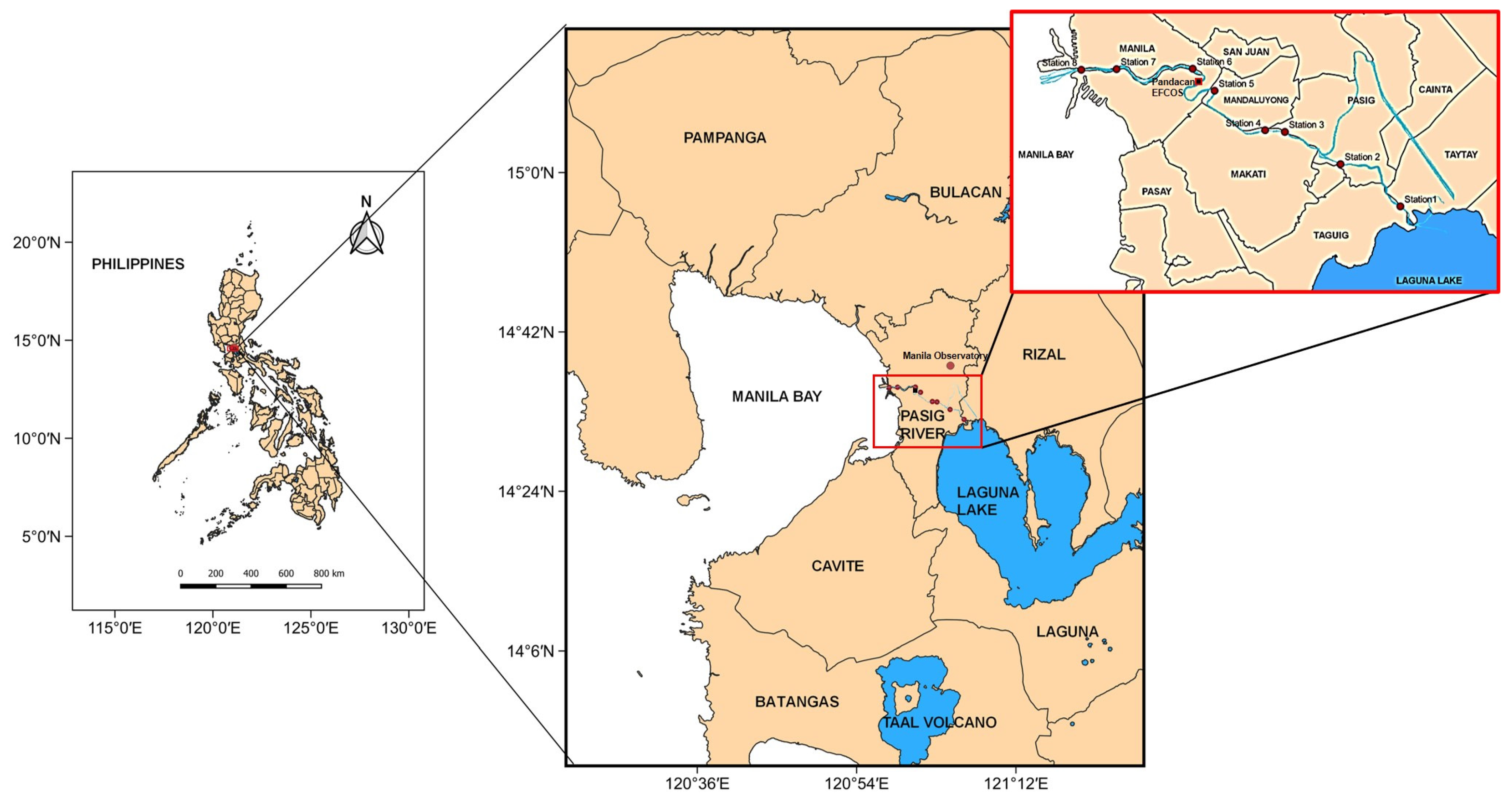
Situated in the province of Batangas, the Taal volcano is approximately 50 km south of Manila (Figure 1). During the 2020 eruption, ashfall from the volcano was experienced in Cavite and Laguna and reached as far as Metro Manila, Bulacan, and Pam-panga (more than 100 km from the source). According to Lagmay et al. [21], initially, the tephra released from the volcano moved southwest before shifting its direction north-northeastward after a few hours [22]. The following day, the smoke and ash from Taal Volcano moved in a southwestward direction [1,3,22]. Dispersed tephra particles with a thickness of < 1 mm were measured in Rizal, Bulacan, and Pampanga, while thicker deposits measuring ≥ 1 mm were reported in southern Metropolitan Manila and some portions of the provinces of Rizal, Cavite, and Laguna [22].
The Pasig River is a major river in this country. It connects two large bodies of water, Laguna Lake, a freshwater ecosystem, and Manila Bay, a saltwater marine ecosystem [23]. The Pasig River stands as one of the prominent waterways in the Philippines, coursing through the heart of the National Capital Region (NCR) and traversing Manila (65 km from the active Taal volcano vent) and its neighboring urban areas. Its expansive reach spans across six distinct cities within Metro Manila. According to the Department of Environmental and Natural Resources (DENR), the river length is approximately 27 km, characterized by an average width ranging from 70 to 120 m and a depth that varies between 2.73 and 4.40 m.
2.2. Data Collection and Database Preparation
Data gathering was performed at the different stations (Table 1) along the main Pasig River. The fieldwork involved the measurement of the flow velocity, turbidity, and water sample collection that were analyzed to determine the total suspended solids (TSS). The data gathering was performed on two separate dates: 25 February 2022 and 2 March 2022. The fieldwork began at the Napindan station and ended at Manila Bay.
The actual sediment concentrations were used for the calibration of the model in order to investigate the occurrence of sediment transport within the river system. Suspended sediment concentrations were determined through laboratory procedures using the water samples collected during the fieldwork.
The laboratory procedure for determining the suspended load within the river began with the preparation of the water samples from each station. The analysis of the water samples was divided into two trials, with each trial having a volume of 250 mL from each sample at each station. The samples were filtered using a Buchner funnel connected to a vacuum pump to ensure that moisture was removed. Furthermore, 0.45-micron filters were used for the analysis of the samples; these were oven-dried at a temperature range of 103 °C to 105 °C for an hour and were subjected to a desiccator for 5 min. The micron filters were weighed together with the petri dish before and after the analysis to compute the suspended load of each water sample. Linear regression was performed to determine the correlation between TSS and on-site turbidity and an R² of 0.8204 was obtained. Equation (1) was used to convert turbidity measurements from FNU to mg/L as follows:
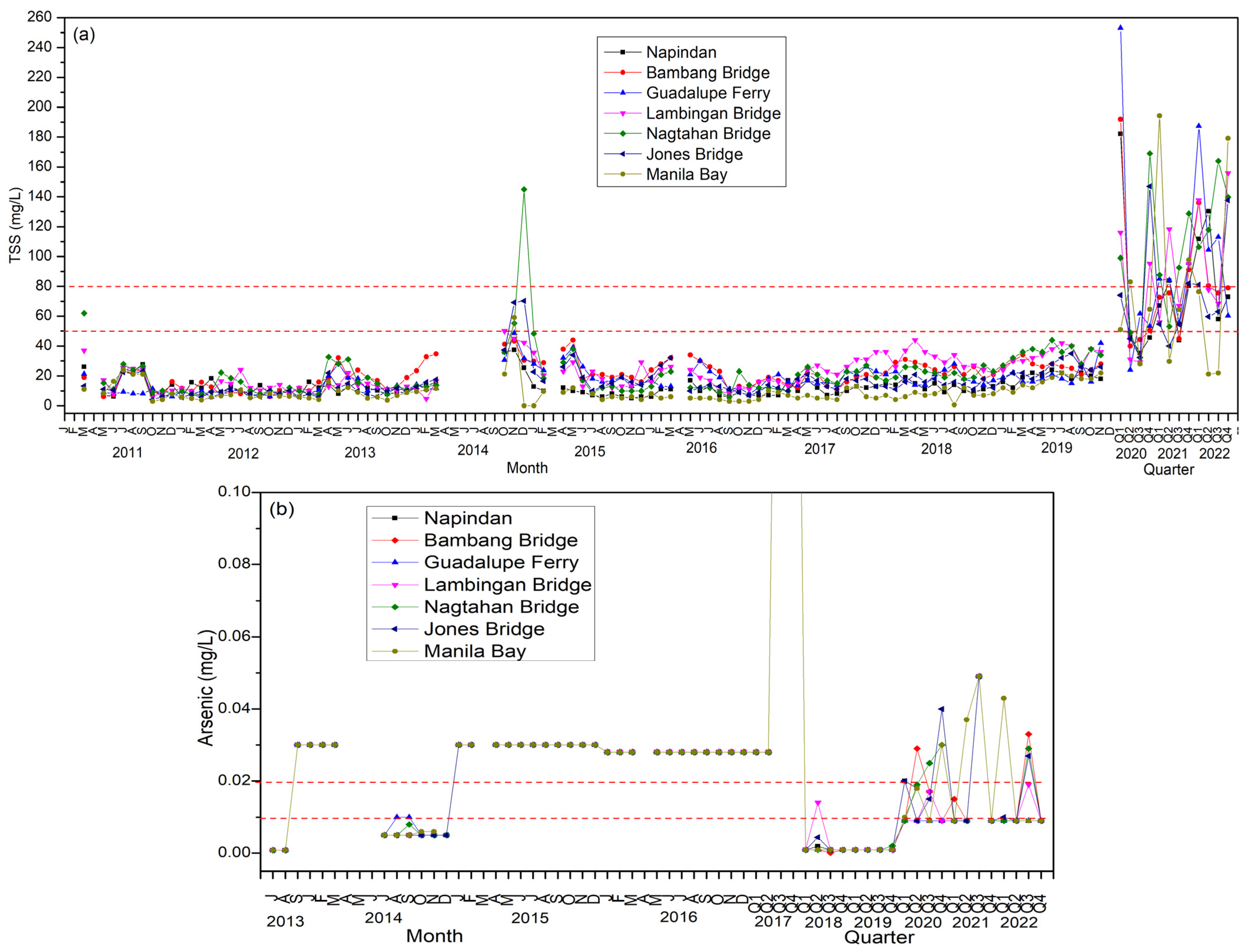
Secondary data of TSS (monthly from 2011 to 2019 and quarterly from 2020 to 2022) and arsenic (monthly from 2013 to 2016 and quarterly from 2017 to 2022) from the Pasig River Unified Monitoring Stations (PRUMS) were obtained. Graphs were created (Figure 2a,b) to represent the monitoring data, and an analysis was conducted to observe trends for the years prior to and after the volcanic eruption.
2.3. Modeling Approach
HEC-RAS (Hydrologic Engineering Center’s River Analysis System) is a widely used software developed by the U.S. Army Corps of Engineers for hydraulic and hydrologic modeling. It is primarily designed for river and open channel flow modeling, but it also has capabilities for sediment transport modeling. In 1D modeling, the flow and sediment transport are considered to occur in a single direction, typically along the main channel of a river or stream. This simplification is appropriate for many situations where the lateral variation of flow and sediment transport is relatively small compared to the longitudinal variation. This study employed HEC-RAS version 6.2.0 to develop a one-dimensional (1D) sediment transport model. The research adopted an unsteady flow approach, necessitating the utilization of various components, including flow velocity, geometry file, plan file, and sediment data for sediment analysis.
2.3.1. Assumptions
Given the limitations of certain data utilized in the modeling process, it was necessary to make certain assumptions and simplifications in order to proceed with the analysis. These adjustments were made to ensure a feasible and accurate representation of the sediment transport model despite the constraints in available information.
- Channel cross-sections were taken by merging the digital elevation model (DEM) and digital terrain model (DTM) files of the Pasig River that were requested from NAMRIA and IFSAR, respectively. Since the DEM file only measures the surface level of the river, it was merged with the DTM file to assume the shape of the cross-section and the depth of the river more accurately.
- Bed gradation for the upstream part of the river is not readily available from the soil analysis performed using the samples obtained through fieldwork. Results from the investigations of related studies were used as supplementary data for this input parameter. The supplementary data obtained were simplified according to the data on hand.
2.3.2. Geometric Model
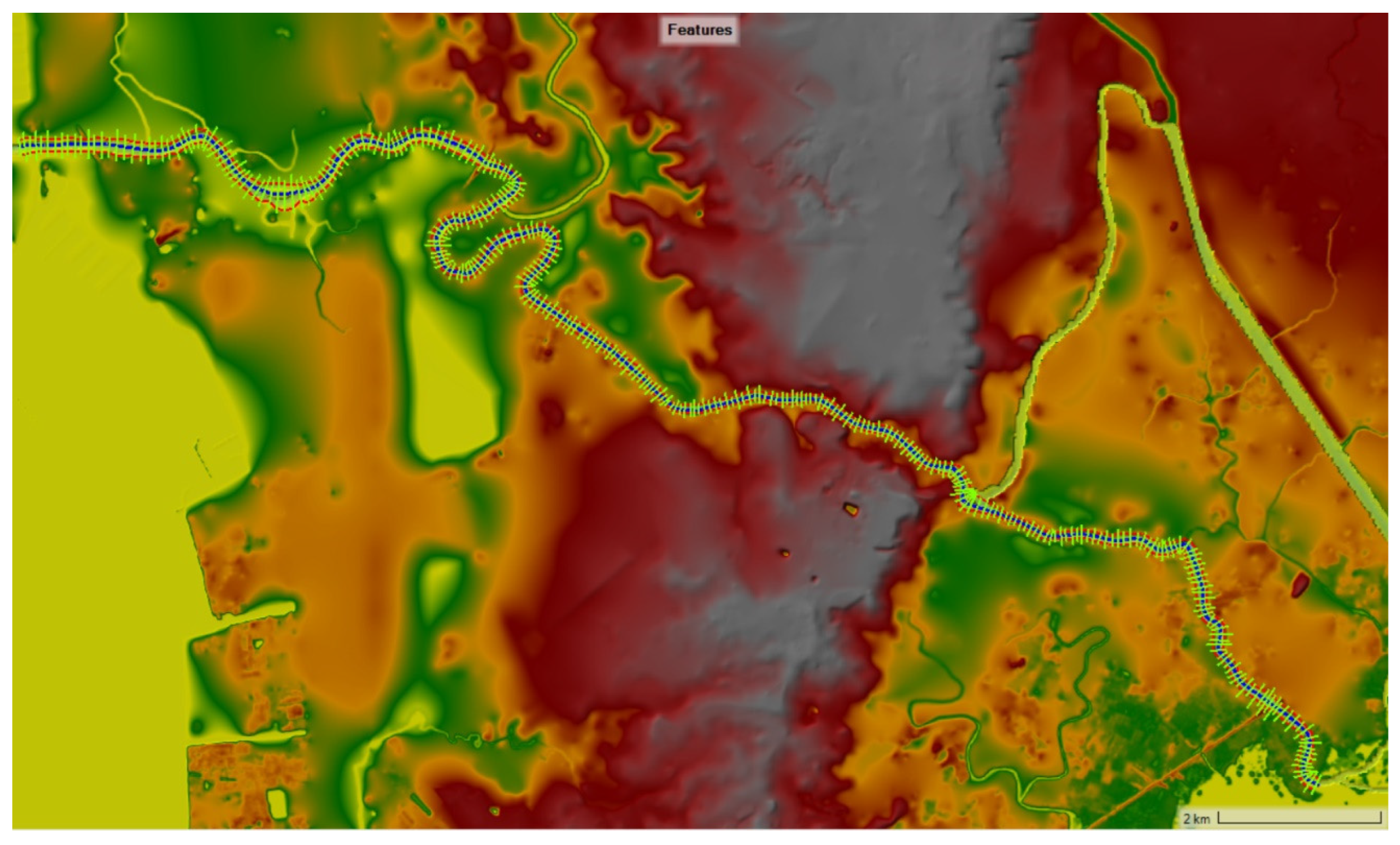
The geometric model of the Pasig River was developed using the RAS mapper feature of HEC-RAS (Figure 3). This study utilized both a DTM and a DEM as base topographies for the simulations. Terrain files like DEM automatically extract topographic variables like basin geometry, stream networks, and flow direction [24,25]. After setting up the terrain files, the stream centerline, flow path, and bank lines were delineated. Afterward, the geometric module was populated with cross-section lines by bisecting the delineated centerline and flow path of the river. A total of 335 cross-section lines were drawn for the model.
2.3.3. Flow Model
The methodological framework for calibration is shown in Figure 4. Hourly tidal-level data were requested from different agencies to serve as the boundary conditions for the upstream and downstream parts of the river. Stage data of the Laguna Lake requested from the Laguna Lake Development Authority (LLDA) were used as the upstream boundary conditions. On the other hand, stage data monitored from the Manila Primary Tide Station requested from NAMRIA were used as the downstream boundary conditions. Using the requested data, a stage hydrograph was used both on the upstream and downstream boundary conditions of the model. Aside from the Marikina River and San Juan River, two of the river’s major tributaries, the effects of the other tributaries were not considered in the flow model. The two rivers were added as internal boundary conditions to account for the impact of their discharge into the Pasig River. Using the flows from these rivers, a uniform lateral inflow hydrograph was included in the model. This boundary condition distributes the flow uniformly along the river reach. This was performed to account for the whole span of the river width, which encompasses more than one cross-section in the model. The results of the hydraulic models were calibrated and compared to the observed stage data from the Effective Flood Control Operation System (EFCOS) at the Pandacan Station.
To ensure that the flow model generated was reliable, the automated Unsteady Flow Manning’s n-value calibration feature of HEC-RAS was also utilized. HEC-RAS performs calculations to adjust the hydraulic characteristics of river reach and roughness coefficients. This feature was utilized by entering an initial set of Manning’s n values for all the cross-sections in the model. The initial set of Manning’s n values were reasonable estimates of the main channel and overbank areas.
The initial set of Manning’s n-values was estimated utilizing Cowan’s (1956) component method, a process involving the analysis of river and surrounding area characteristics using Google Earth version 9.162.0.2. This estimation considered various channel morphology conditions, encompassing the degree of irregularity in the channel cross-section, variations in cross-sectional shape and area, the relative impact of obstructions and vegetation, and the extent of meandering in the river line.
The calibration of the model was considered complete when the simulated stage data at the Pandacan Station closely mirrored the observed stage data. This alignment between simulated and observed data signified the successful adjustment of model parameters, indicating a robust calibration process.
2.3.4. Sediment Model
Sediment analysis was performed on the data gathered on 25 February 2022 when an accurate and calibrated hydraulic model was generated. The input parameters used for the model were the following: sediment transport function, fall velocity, the grain-size sorting method, Manning’s roughness, channel bed gradations, and computational options (time steps) (Figure 5).
Among the listed input parameters, specific model parameters in HEC-RAS, such as the movable bed limits, were systematically investigated beyond their default settings during the sediment calibration process. The sensitivity analysis of the model involved identifying the model parameters that generated sediment concentration results most closely aligned with the observed data. To reduce the number of simulations performed on the model, the Rubey fall velocity function and the Exner 5 size sorting method were chosen based on the inherent characteristics of the river.
The bed gradations used as input for the model came from the results of the soil analysis of the collected samples on the river, using the standard hydrometer method. These were supplemented by the results of the sieve analysis performed in the study of Belo [22].
To assess the reliability of the simulated sediment concentration from the model, the simulation results were compared with observed data collected at various sampling stations along the river. The calibration parameter employed for evaluating the model is the observed sediment concentration. These results were evaluated using statistical indices that can prove the reliability of the developed model. The transport function that gave the most accurate results was used for the validation of the model.
2.4. Model Evaluation
This study uses different statistical indices to evaluate the model generated using HEC-RAS. The coefficient of determination (R2) is one of the most widely used statistical indices for model evaluation. It describes the degree of collinearity between simulated and observed data. The index of agreement (d) was developed by Willmott [26] as a standardized measure of the degree of model prediction error. Legates and McCabe [27] suggest that the statistical index can be used as a substitute for R2 to identify the degree to which model predictions are error-free. For this study, this statistic served as a supplementary index to the calculated R2 values.
The Nash–Sutcliffe efficiency (NSE) is a normalized statistic that determines the relative magnitude of the residual variance known as the “noise” compared to the measured data variance known as the “information” [28]. Values of this statistic range between −∞ and 1.0, with the optimal value being 1.
PBIAS assesses the normal tendency of simulated data to differ from its observed counterparts. This statistic can account for measurement uncertainty [29] and aid in the identification of average model simulation bias [30]; the optimal value is 0.0, with low-magnitude values indicating accurate model simulation. The resulting positive values of the statistical index indicate that the model underestimates the measured values, whereas negative values indicate overestimation [31].
RSR is the ratio between the root mean square error (RMSE) of simulated and observed values and the standard deviation of observed data. It standardizes the RMSE using the observation’s standard deviation. RSR varies from the optimal value of 0.0 to a large positive value. Lower values of RSR indicate a lower RMSE, resulting in better model simulation performance.
where n is the total number of observations and the constituent beings evaluated is the ith observed value, is the ith simulated value, and is the mean of observed data.
3. Results and Discussion
3.1. Total Suspended Sediment and Arsenic in Pasig River
Historical data of TSS in the Pasig River spanning from 2011 to 2022 are presented in Figure 2a. These findings reveal a noteworthy increase in TSS levels following the volcanic eruption. Notably, from 2020 to 2022, TSS concentrations in all main Pasig River stations (Napindan Bridge, Bambang Bridge, Guadalupe Ferry, Lambingan Bridge, Nagtahan Bridge, and Jones Bridge) exceeded the allowable 80 mg/L for Class C water, as stipulated in the DENR Administrative Order (DAO) 2016–08 Water Quality Guidelines and General Effluent Standards 2016. During field measurements performed by the PRCMO, algal bloom was evident in the stations along the Pasig River. Being exposed to volcanic ash, which is high in trace metals like iron and nutrients like nitrogen, phosphorus, and silicon that are readily available for phytoplanktons, previous studies have shown the direct correlation between volcanic eruption and algal bloom [14]. Algal bloom, along with dredging and ongoing constructions, may have affected the TSS in the Pasig River.
In the 12 quarters spanning 2020 to 2022, the Manila Bay station exceeded the permissible 50 mg/L standard in only 4 quarters. Elevated sediment levels in both the bay and coastal areas present challenges to ship navigability, impacting trading routes. The accumulation of substantial sediment deposits at river mouths not only harbors toxic pollutants but also diminishes the flood-carrying capacities of channels.
Looking ahead, the anticipated sea level rise is expected to bring about changes in tidal range, potentially leading to more frequent and severe flooding scenarios. In the coming decades, flood thresholds previously surpassed by the combined effects of freshwater and saltwater may be exceeded solely by tidal influences [32]. Presently, large ships are unable to approach the Pasig River closely due to concerns about turbines encountering bottom sediments, resulting in potential damage and malfunctions.
One proactive approach to address these issues is the modeling of sediment transport. By doing so, preemptive solutions can be developed, mitigating the need for reactive measures. It is crucial to refine coastal adaptation policies as early as possible, particularly given the existing shortcomings in government policy structures and water quality management. This proactive stance can contribute to more effective and sustainable solutions for the challenges posed by sediment accumulation in Manila Bay and its surrounding areas.
A similar pattern emerged for arsenic (As) levels, which showed a continuous increase since 2020 (Figure 5). Several stations had As levels that were higher than the 0.02 mg/L allowable minimum for Class C freshwater and the 0.01 mg/L allowable level for Class SB marine water at Manila Bay. A significant environmental concern arising from volcanic eruptions is the release of substantial volumes of ashfall containing hazardous elements such as arsenic [33]. Arsenic, a heavy metal, naturally occurs in the environment due to weathering on crustal rocks and volcanic emissions [34]. Prior research indicates that hydrothermal systems located at or near tectonic plate convergent boundaries, like those found in the Philippines, tend to discharge geothermal water with elevated arsenic content [35,36].
Recent studies have assessed arsenic levels in surface sediments in the Arabian Gulf, encompassing areas like Half Moon Bay and Al Buhairah Bay. While the current Arsenic (As) hazard index indicated non-carcinogenic risks, it was found that the lifetime cancer risk associated with arsenic exposure was higher for children compared to adults [34]. This underscores the importance of understanding and monitoring the arsenic distribution and exposure in areas affected by volcanic activities, emphasizing the need for comprehensive risk assessments and protective measures, especially for vulnerable populations such as children.
Arsenic enters water sources through the dissolution of minerals and ores, industrial discharges, and atmospheric deposition. It poses significant toxicity to humans, and the contamination of water and soil by arsenic poses a substantial risk to agriculture, fisheries, and various industries [37]. Arsenic levels from 26 locations in Batangas near the volcano from 2020 to 2021 were found to be significantly and consistently higher than the World Health Organization (WHO) and Philippine National Standards for Drinking Water (PNSDW) 10 ppb limit. The 2020 levels were comparatively higher than those of 2019, which is believed to be caused by a more active Taal volcano [38]. These findings, in conjunction with various other factors, served as primary motivations for the initiation of the study.
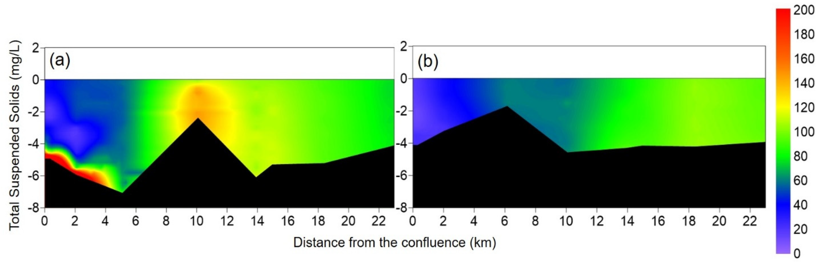
To analyze the sediment transport in a smaller time step, separate field data gatherings were conducted on 25 February 2022 and 3 March 2022 at neap and spring tide, respectively. Results showed that the TSS was well mixed in the entire main Pasig River (Figure 6). Given this information, 1-D modeling is possible for sediment transport using HEC-RAS. Empirical equations may provide a more straightforward approach and are particularly useful when detailed data are limited. However, since there were on-site and secondary data that were available, the numerical model utilizing HEC-RAS that required calibration and verification was chosen. The model could be further used for other scenarios like rare estuarine occurrences for this well-mixed estuary which lacked published research made available to the public.
3.2. Flow and Sediment Model Calibration and Validation
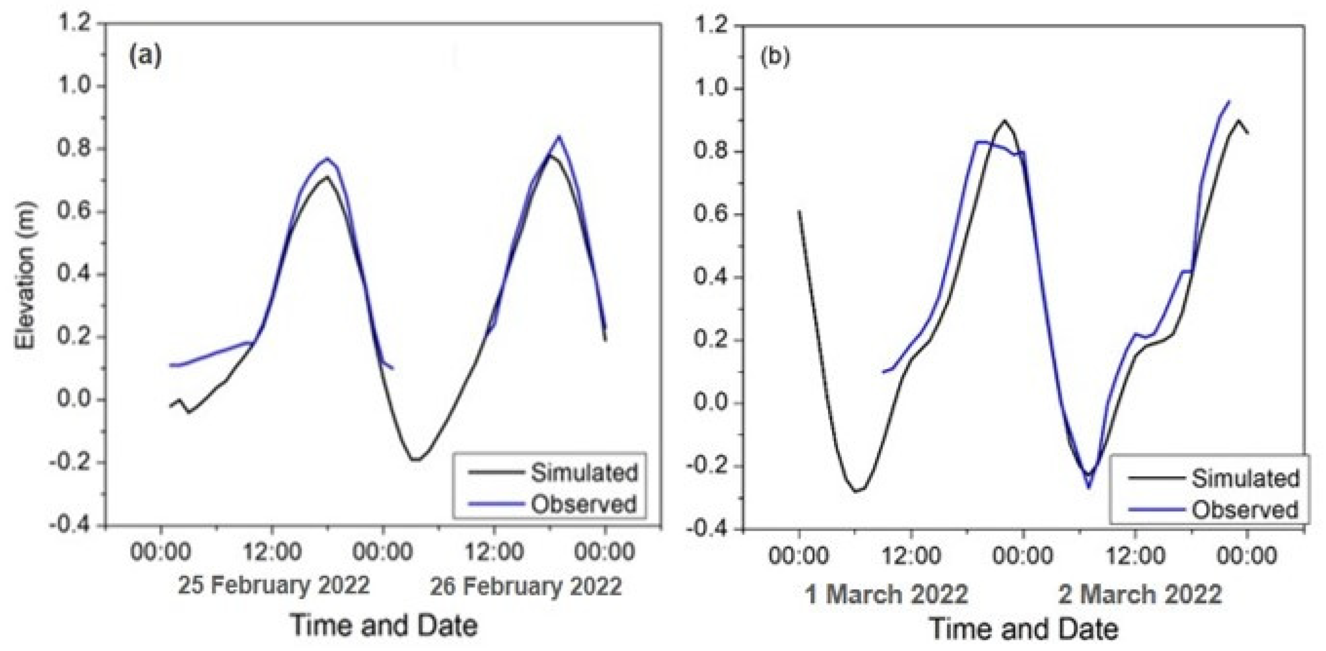
The results of the calibration of the flow model involve the comparison of the simulated and observed data on the Pandacan Station. Cowan’s (1956) component method of estimating Manning’s n values was used in determining the values of ‘n’ used as input for the model. It was determined that the ‘n’ values for the river range from 0.02–0.0455; whereas the highest Manning’s coefficient value was observed at the mid-stream part of the river where the presence of vegetation is low and the effects of obstruction are the highest. Calibration results of the flow model show that the stage data simulated follow that of the observed data in the Pandacan Station.
The flow model was calibrated during the neap tide on 25–26 February 2022. With an average error of 0.0567 m (Figure 7a), a 5.7 cm difference between the simulated and observed water levels was determined. The flow model was then validated during the spring tide on 1–2 March 2022 (Figure 7b), resulting in an average error of 0.0882 m or an 8.8 cm difference between the simulated and observed water levels.
Once the flow model was calibrated, sediment analysis and validation runs or simulations were performed using the data gathered. Based on the simulations performed during the sensitivity analysis of the model, it was observed that the sediment concentration results are sensitive to the modification of movable bed limits and bed gradation.
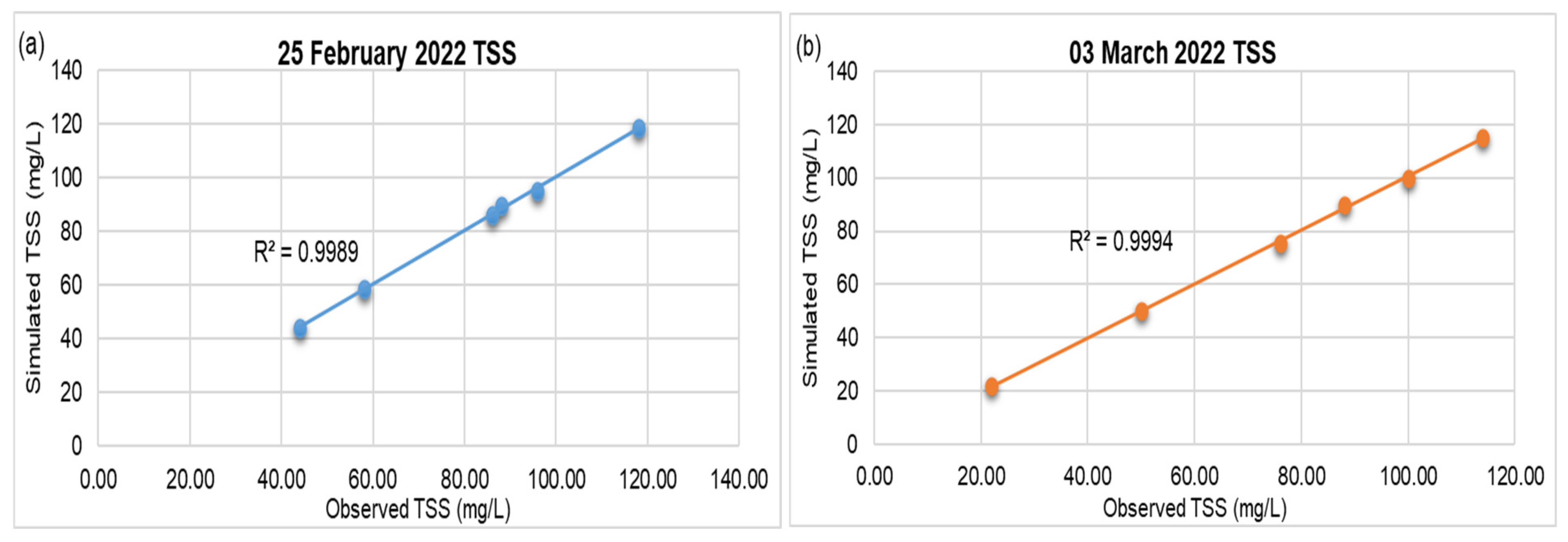
During model calibration, Copeland’s simulation of Laursen’s equation produced the most accurate results. Statistical evaluations using the aforementioned function showed that the robustness of the model is acceptable (Table 2). Having been able to simulate results with low error variance against the observed data indicates accurate model simulation and acceptable model performance in predicting values. The validation of the model was performed by simulating the sediment concentration of the river on 3 March 2022.
The validation of the model also produced good model performance results based on the obtained statistical parameters and coefficient of determination (Figure 8). As opposed to the results of its initial calibration, the final model developed indicates an overestimation of the simulated values compared to the measured ones. This is shown by the negative results of the evaluation of the model using the PBIAS index. Since the sediment concentration simulated in this study is most sensitive to movable bed limits, the overestimation of the results of the model can be attributed to this.
According to the model, a peak sediment concentration of 120.63 mg/L was predicted in Station 1 during the neap tide of the dry season (25 February 2022). There was a recorded Taal volcano eruption on 29–30 January 2022. The trend of TSS was decreasing from upstream to downstream stations. The PRUMS first-quarter report mentioned that the TSS levels increased compared with the previous quarter due to elevated levels of fecal coliform from increased discharges from household, industrial, and commercial establishments as a result of less strict quarantine restrictions. There was also sheet piling and oil and grease sludge in tributaries. Lastly, there were notable observations of green algae in the main Pasig River, which is attributed to elevated amounts of phosphate. A study on river system responses to volcanic eruptions by Siringan et al. [14] found that harmful algal blooms plagued Sorsogon Bay after the Mount Bulusan eruption due to increased dissolved silica in rivers and estuaries. It is not within the scope of this study to relate algal bloom to elevated TSS levels post volcanic eruption. However, this is a good finding that will be relevant to future studies.
The final combination of parameters used to create a well-calibrated and validated model is outlined below.
Utilizing Copeland’s version of Laursen’s equation as the transport function, the model is designed to be versatile, accommodating grain sizes ranging from fine silt to coarse gravels. Consequently, the majority of the specified grain classes for the model are well-suited within its applicable range.
The applicable conditions of the Rubey fall velocity method were also in line with the actual environment of the Pasig River. This equation has been shown to be adequate for silt, sand, and gravel grains. Based on the bed gradation data used for the model, most of the bed material consists of silt and sand.
Exner 5 was employed as a sorting method for evaluating the thickness of the active layer and vertical bed layer. This approach—which HEC RAS used by default—allows for the formation of a rougher layer to prevent the erosion of deeper materials.
The Equilibrium Load was used as a sediment boundary condition since there were no available data for sediment load as a boundary that could be used. This condition specifies the inflow sediment load as the equilibrium sediment load in the model, which is an approximation that essentially assumes a zero-gradient concentration normal for the boundary [39].
Several studies have focused on flow modeling and estimating total suspended sediments in the Pasig River. One such study developed a rainfall-runoff and inundation model for the Marikina-Pasig River Basin, employing an adaptive mesh refinement scheme to simulate the impact of Typhoon Ketsana in 2009 [40]. The model exhibited R2 values of 0.875 and 0.275 for flood and no flood area identification, respectively, based on the digital terrain model and digital surface model.
In another study, the estimation of Total Suspended Solids (TSS) in the Pasig River was conducted using satellite images and empirical ordinary least-squares regression models [41]. However, this model faced challenges as the root mean square error (RMSE) obtained was notably high. Furthermore, the model failed the multicollinearity test, contributing to an increase in overall standard errors in its predictions.
3.3. 2020 Model Development and Simulation Results
Sediment concentrations in surface waters are greatly influenced by the prevailing tides and flows. Based on the related literature on the flow of the river, Paronda et al. [42] mentioned that the Pasig River discharges at a faster rate during low tide, so contaminants and particles are washed out straight toward Manila Bay. This is a similar result to our findings during our fieldwork. Freshwater from Laguna Lake flows faster during low tide and slows down during high tide, and the tributaries have very low flow during the dry season. Therefore, low flow rates on the river could allow the settlement of waste and sludge in the river, which results in cloudy water that consequently accumulates on the riverbed.
The PRUMS report indicated a drastic TSS increase in the first quarter of 2020. The sudden increase in TSS concentration may be due to the ongoing extensive restoration and building of significant bridges in close proximity to the sampling locations, including Batasan Bridge, Tumana Bridge, and Lambingan Bridge. Additionally, various flood control initiatives have contributed to the disturbance of the riverbed, leading to the widespread dispersion of debris and tiny particles throughout the waterways. Although significant changes were observed in the sediment concentration of the Pasig River before and after the Taal eruption, most of these changes could also be related to the variations in tide, season, and flow in the river system.
To further investigate the effects of the eruption on the river system, a sediment model for February 2020 was created. Due to the limited data from secondary sources, inputs used for the development of this model were assumed by utilizing the pre- and post-eruption sediment models generated in the earlier parts of this study and the discharges from two EFCOS tributaries along the main Pasig River.
Using the calibrated model, the results of the simulation were compared with the observed TSS concentration data from PRUMS on 20 February 2020. The statistical evaluation of the model showed a good performance based on the resulting statistical indices, just like the pre- and post-eruption models developed (Table 3). The model generated showed that it was sensitive to changes in movable bed limits and bed gradation.
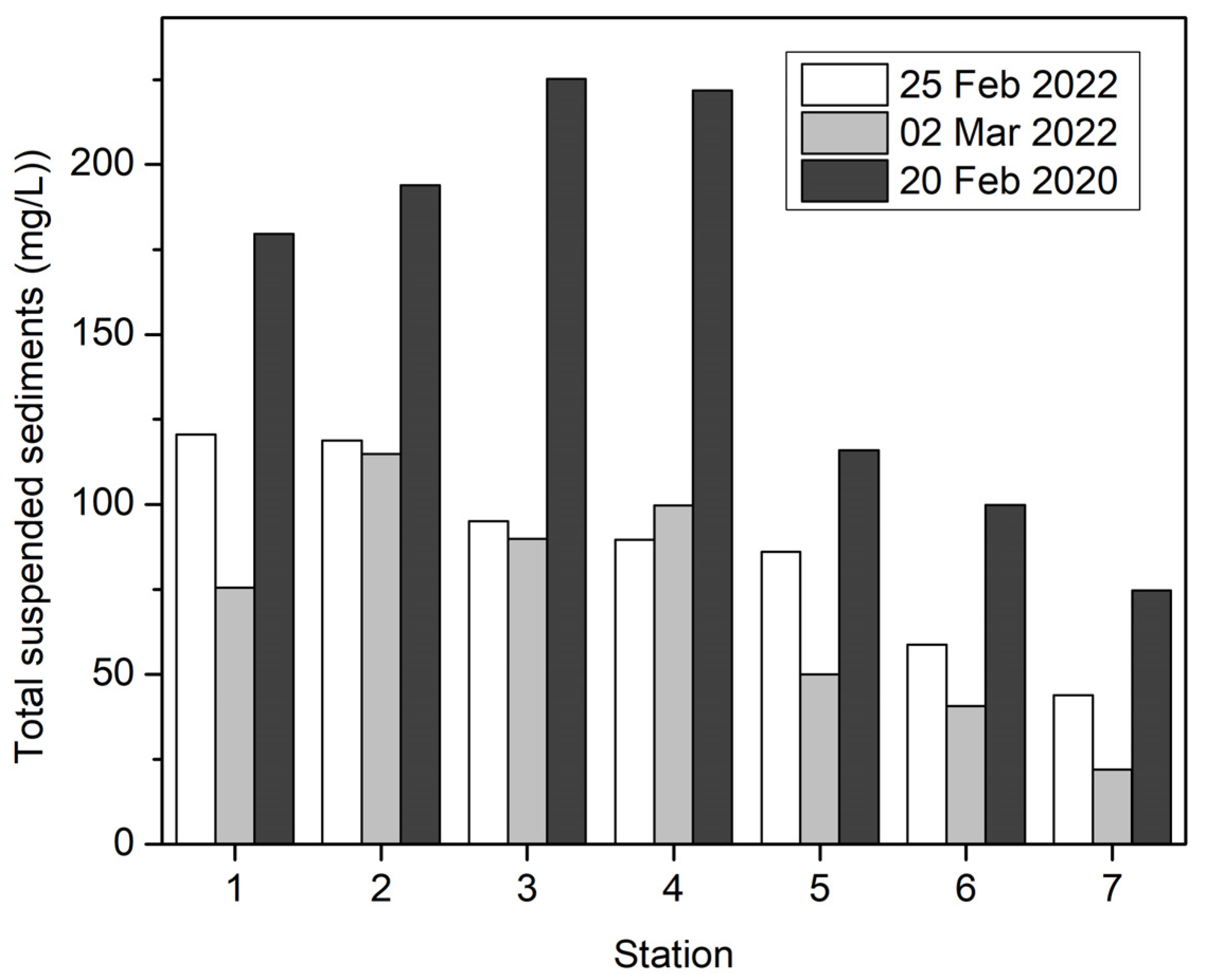
The simulated sediment concentration of the 2020 model was then compared to the concentration values two years after the eruption. The resulting sediment concentration values were higher than the TSS after two years (Figure 9). This significant increase in sediment concentration a month after the eruption may still be attributed to the Taal volcano activity. It can be assumed that the Taal Volcano eruption contributed to this significant increase since an increase in the turbidity of Laguna Lake (upstream freshwater source) was reported immediately after the eruption.
Kataoka et al. [43] noted sustained transportation of suspended volcaniclastic sediment in the Akagawa–Nigorigawa River system that lasted for at least 19 months upon studying the 2014 phreatic eruption of the Ontake Volcano, a relatively small-scale eruption event with a Volcanic Explosivity Index (VEI) value of 1–2. Rain-triggered lahar and pyroclastic density current deposits positioned at the head of the river were attributed as the reason for the high sediment concentration and transportation observed in the river system.
This assumption, however, still needs further investigation. Various studies that investigate the effects of an eruption on river systems involve determining the characteristics of plume deposits and sediment yields [43]. Other investigations also indicated that post-eruption sediment yields due to significant geomorphic changes are several hundred times greater than pre-eruption yields [44,45].
Given that the study lacks the necessary methodologies for investigating the presence of eruptive materials in the river’s sediment loads, the simulated results of the generated models for this study can be utilized as benchmark information to further investigate if sediment loads within the river contain volcanic eruptive material from Taal.
The high R2 values achieved during both the calibration and validation phases attest to the model’s commendable accuracy. While the model proves effective for dry season sediment transport dynamics, its applicability extends to rivers and estuaries influenced by tides, demonstrating favorable outcomes across neap and spring tide conditions. However, attempts to model the wet season yielded underestimated Total Suspended Solids (TSS) results, possibly attributed to the varying bottom sediments in the Pasig River during different seasons [46].
To address this limitation, recalibration of the model, particularly concerning Manning’s roughness coefficient, may be necessary. This adjustment could enhance the model’s performance and ensure its reliability across diverse seasonal dynamics.
Despite this seasonal variability challenge, the model holds significant relevance for future simulations, particularly in predicting hydraulic flows for inundation and conducting flood risk assessments. Furthermore, its utility extends to the analysis of sediment transport dynamics. In the Pasig River, sediments exhibit higher concentrations of total metals during the summer season, attributed to reduced flow disturbances [47]. Therefore, the model stands as a valuable tool for future studies, addressing sedimentation-related issues, and other geological applications—especially considering the continued unrest of the Taal Volcano even after four years [48].
4. Conclusions
Sediment transport modeling is an arduous task that requires careful and skillful practice, time, and patience. Despite the limitations and simplifications made, sediment transport models were successfully developed. With lacking historical data, it was made feasible to model flow and sediment transport by establishing a connection between the upstream and downstream boundary conditions of 1D river flow using HEC-RAS. Statistical indices and performance ratings developed for model evaluation were used to calibrate and validate the developed model. The results of the simulations passed all the statistical criteria during their evaluation, which matches the observed sediment concentration data obtained after the laboratory analysis of fieldwork samples. An R2 value of 0.9994 was obtained for the post-eruption model during the calibration of the model using the Laursen transport function.
The sediment concentration results of the models were investigated by accounting for the variations in the river’s flow rates, tides, and seasons. It was observed that the sediment concentration of the river during the dry season peaked at 120.63 mg/L in Station 1. It was also observed, based on the simulated data, that the water was stagnant in the upstream part of the river during the neap tide of the dry season.
By finalizing the study with simulations determining the sediment concentration on the river in February 2020, the results showed a significant increase in sediment concentrations at all selected stations of the river. The values of sediment concentrations peaked at 225.15 mg/L in Station 3, from which it can be assumed that the eruption, algal bloom, and other factors like dredging and construction may have caused this increase. The increase in sediment concentration in 2020 could also be attributed to the continuous large-scale rehabilitation and construction of major bridges such as Batasan Bridge, Tumama Bridge, and Lambingan Bridge (Station 5). Flood control projects may have also caused disturbance of the riverbed and further dispersion of debris and minute particles along waterways. The following are recommended:
- (1)
- Use of other software to investigate the same case as the current study and compare its findings to observed data.
- (2)
- Conduct more field measurements and perform simulations using the present model under different conditions, climatological data, water level, and discharge as input.
- (3)
- Study the same case simulations at much earlier dates prior to the volcanic eruption using the present model.
The need to further investigate if the Taal Volcano eruption influences the changes within the Pasig River comes from the fact that water bodies that have been physically and chemically contaminated as a result of a volcanic eruption are lethal to riverine biota and can have an impact on the quality of the drinking water supply and irrigation use. While the study is constrained to the dry season, the model proves applicable to sediment hydrodynamic simulations, encompassing scenarios such as sediment resuspension due to dredging or potential large volcanic eruptions, considering the ongoing unrest of Taal Volcano. The model’s adaptability makes it a valuable tool for predicting sediment dynamics in various dynamic conditions.
Future research endeavors could leverage the model for hydraulic flow simulations, specifically in the context of rainfall-runoff inundation and comprehensive flood risk assessments. An intriguing avenue for investigation lies in directing studies towards flood threshold exceedance in downstream areas, particularly those heavily silted, and at critical points such as river mouths or surrounding Manila Bay. These locations are significant as tidal flood regimes may undergo shifts with rising sea levels and occasional astronomical events. Additionally, the model could play a crucial role in addressing various sediment-related issues, offering insights into the intricate dynamics of sedimentation in these environmentally sensitive areas.
With the efforts being made to improve water quality on the Pasig River, understanding the factors that contribute to its sediment transport would help in developing strategies for managing and mitigating problems and hazards posed by the said occurrence.
Author Contributions
Conceptualization, J.C.C.; methodology, J.C.C., H.L.A. and S.H.; software, H.L.A.; validation, H.L.A. and S.H.; formal analysis, H.L.A.; investigation, H.L.A.; resources, J.C.C. and K.Y.; data curation, J.C.C.; writing—original draft preparation, J.C.C. and H.L.A.; writing—review and editing, J.C.C., H.L.A., S.H. and K.Y.; visualization, J.C.C. and H.L.A.; supervision, J.C.C.; project administration, J.C.C.; funding acquisition, J.C.C. All authors have read and agreed to the published version of the manuscript.
Funding
This work was funded by the UP System Enhanced Creative Work and Research Grant (ECWRG-2021-1-8R).
Data Availability Statement
Data are contained within the article.
Acknowledgments
The authors would like to acknowledge the Pasig River Coordinating and Management Office for the provision of the Pasig River water quality quarterly and annual reports. The authors also express special thanks to the Pasig River Ferry Service Office for the ferry boat arrangement and support during the conduct of the field works. To everyone who helped during the conduct of field measurements, laboratory analysis, to Engr. Princess Bautista for the map making, and to students and interns who performed data encoding, thank you for making this project possible.
Conflicts of Interest
The authors declare no conflicts of interest.
References
- UN Office for the Coordination of Human Affairs [OCHA]. Philippines: Taal Volcano Eruption Displacement Snapshot (As of 15 January 2020). Reliefweb. Available online: https://reliefweb.int/report/philippines/philippines-taal-volcano-eruption-displacement-snapshot-15-january-2020 (accessed on 10 October 2022).
- UN Office for the Coordination of Human Affairs [OCHA]. Philippines: 2020 Significant Events Snapshot (As of 14 January 2021). Reliefweb. Available online: https://reliefweb.int/report/philippines/philippines-2020-significant-events-snapshot-14-january-2021 (accessed on 10 October 2022).
- Manila Observatory. Impacts of Taal Volcano Phreatic Eruption (12 January 2020) on the Environment and Population: Satellite-Based Observations Compared with Historical Records. Available online: https://www.observatory.ph/2020/04/20/impacts-of-taal-volcano-phreatic-eruption-12-january-2020-on-the-environment-and-population-satellite-based-observations-compared-with-historical-records/ (accessed on 13 January 2022).
- International Federation of Red Cross and Red Crescent Societies [IFRC]. Philippines: Taal Volcano Eruption—Final Report. Reliefweb. Available online: https://reliefweb.int/report/philippines/philippines-taal-volcano-eruption-final-report-n-mdrph043 (accessed on 10 October 2022).
- Thouret, J.-C.; Oehler, J.-F.; Gupta, A.; Solikhin, A.; Procter, J.N. Erosion and Aggradation on Persistently Active Volcanoes—A Case Study from Semeru Volcano, Indonesia. Bull. Volcanol. 2014, 76, 857. [Google Scholar] [CrossRef]
- Pickarski, N.; Kwiecien, O.; Litt, T. Volcanic Impact on Terrestrial and Aquatic Ecosystems in the Eastern Mediterranean. Commun. Earth Environ. 2023, 4, 167. [Google Scholar] [CrossRef]
- Lim, J.A. The Philippine Economy during the COVID Pandemic; Ateneo Center for Economic Research and Development, Ateneo de Manila University: Quezon City, Philippines, 2020. [Google Scholar]
- Santos, J.; Roquel, K.I.D.Z.; Lamberte, A.; Tan, R.R.; Aviso, K.B.; Tapia, J.F.D.; Solis, C.A.; Yu, K.D.S. Assessing the Economic Ripple Effects of Critical Infrastructure Failures Using the Dynamic Inoperability Input-Output Model: A Case Study of the Taal Volcano Eruption. Sustain. Resilient Infrastruct. 2023, 8, 68–84. [Google Scholar] [CrossRef]
- National Economic and Development Authority [NEDA] Region IV-A. CALABARZON Rehabilitation and Recovery Program for Taal Volcano Eruption. Available online: https://serp-p.pids.gov.ph/publication/public/view?slug=calabarzon-rehabilitation-and-recovery-program-for-taal-volcano-eruption (accessed on 22 November 2022).
- Ancheta, J.R.; Gamayo, G.V. Women in Disasters: Unfolding the Struggles of Displaced Mothers in Talisay, Batangas during the Taal Volcano Eruption and the Pandemic. Rupkatha 2022, 14, 1–10. [Google Scholar] [CrossRef]
- Lebrato, M.; Wang, Y.V.; Tseng, L.-C.; Achterberg, E.P.; Chen, X.-G.; Molinero, J.-C.; Bremer, K.; Westernströer, U.; Söding, E.; Dahms, H.-U.; et al. Earthquake and Typhoon Trigger Unprecedented Transient Shifts in Shallow Hydrothermal Vents Biogeochemistry. Sci. Rep. 2019, 9, 16926. [Google Scholar] [CrossRef] [PubMed]
- Lallement, M.; Macchi, P.J.; Vigliano, P.; Juarez, S.; Rechencq, M.; Baker, M.; Bouwes, N.; Crowl, T. Rising from the Ashes: Changes in Salmonid Fish Assemblages after 30 Months of the Puyehue–Cordon Caulle Volcanic Eruption. Sci. Total Environ. 2016, 541, 1041–1051. [Google Scholar] [CrossRef] [PubMed]
- Lacaux, J.P.; Tourre, Y.M.; Vignolles, C.; Ndione, J.A.; Lafaye, M. Classification of Ponds from High-Spatial Resolution Remote Sensing: Application to Rift Valley Fever Epidemics in Senegal. Remote Sens. Environ. 2007, 106, 66–74. [Google Scholar] [CrossRef]
- Siringan, F.P.; Racasa, E.D.R.; David, C.P.C.; Saban, R.C. Increase in Dissolved Silica of Rivers Due to a Volcanic Eruption in an Estuarine Bay (Sorsogon Bay, Philippines). Estuaries Coast 2018, 41, 2277–2288. [Google Scholar] [CrossRef]
- Hayes, S.K.; Montgomery, D.R.; Newhall, C.G. Fluvial Sediment Transport and Deposition Following the 1991 Eruption of Mount Pinatubo. Geomorphology 2002, 45, 211–224. [Google Scholar] [CrossRef]
- Manzella, I.; Bonadonna, C.; Phillips, J.C.; Monnard, H. The Role of Gravitational Instabilities in Deposition of Volcanic Ash. Geology 2015, 43, 211–214. [Google Scholar] [CrossRef]
- Rose, W.I.; Durant, A.J. Fine Ash Content of Explosive Eruptions. J. Volcanol. Geotherm. Res. 2009, 186, 32–39. [Google Scholar] [CrossRef]
- Eliasson, J. New Model for Dispersion of Volcanic Ash and Dust in the Troposphere. Int. J. Geosci. 2020, 11, 544–561. [Google Scholar] [CrossRef]
- Cruz, M.T.; Simpas, J.B.; Holz, R.; Yuan, C.-S.; Bagtasa, G. Characteristics of Particulate Matter during New Year’s Eve Fireworks and Taal Volcano Ashfall in Metro Manila on January 2020. Urban Clim. 2023, 50, 101587. [Google Scholar] [CrossRef]
- Trenberth, K.E.; Dai, A. Effects of Mount Pinatubo Volcanic Eruption on the Hydrological Cycle as an Analog of Geoengineering. Geophys. Res. Lett. 2007, 34, L15702. [Google Scholar] [CrossRef]
- Lagmay, A.M.F.; Balangue-Tarriela, M.I.R.; Aurelio, M.; Ybañez, R.; Bonus-Ybañez, A.; Sulapas, J.; Baldago, C.; Sarmiento, D.M.; Cabria, H.; Rodolfo, R.; et al. Hazardous Base Surges of Taal’s 2020 Eruption. Sci. Rep. 2021, 11, 15703. [Google Scholar] [CrossRef]
- Balangue-Tarriela, M.I.R.; Lagmay, A.M.F.; Sarmiento, D.M.; Vasquez, J.; Baldago, M.C.; Ybañez, R.; Ybañez, A.A.; Trinidad, J.R.; Thivet, S.; Gurioli, L.; et al. Analysis of the 2020 Taal Volcano Tephra Fall Deposits from Crowdsourced Information and Field Data. Bull. Volcanol. 2022, 84, 35. [Google Scholar] [CrossRef] [PubMed]
- Belo, L.P. Measurement of the Sediment Oxygen Demand in Selected Stations of the Pasig River Using a Bench-Scale Benthic Respirometer. Master’s Thesis, Environmental Engineering and Management–De La Salle University, Manila, Philippines, October 2008. [Google Scholar]
- Joshi, N.; Lamichhane, G.R.; Rahaman, M.M.; Kalra, A.; Ahmad, S. Application of Hec-Ras to Study the Sediment Transport Characteristics of Maumee River in Ohio. In Proceedings of the World Environmental and Water Resources Congress 2019, Pittsburgh, Pennsylvania, 19–23 May 2019; American Society of Civil Engineers: Reston, VA, USA, 2019; pp. 257–267. [Google Scholar]
- Akhtar, M.N.; Anees, M.T.; Bakar, E.A. Assessment of the Effect of High Tide and Low Tide Condition on Stream Flow Velocity at Sungai Rompin’s Mouth. In Proceedings of the IOP Conference Series: Materials Science and Engineering, 6th International Conference of Global Network for Innovative Technology (IGNITE), Penang, Malaysia, 2–3 December 2019. [Google Scholar]
- Willmott, C.J. On the Validation of Models. Phys. Geogr. 1981, 2, 184–194. [Google Scholar] [CrossRef]
- Legates, D.R.; McCabe, G.J. Evaluating the Use of “Goodness-of-fit” Measures in Hydrologic and Hydroclimatic Model Validation. Water Resour. Res. 1999, 35, 233–241. [Google Scholar] [CrossRef]
- Nash, J.E.; Sutcliffe, J.V. River Flow Forecasting through Conceptual Models Part I—A Discussion of Principles. J. Hydrol. 1970, 10, 282–290. [Google Scholar] [CrossRef]
- Harmel, R.D.; Smith, P.K.; Migliaccio, K.W. Modifying Goodness-of-Fit Indicators to Incorporate Both Measurement and Model Uncertainty in Model Calibration and Validation. Trans. ASABE 2010, 53, 55–63. [Google Scholar] [CrossRef]
- Moriasi, D.N.; Arnold, J.G.; Liew, M.W.V.; Bingner, R.L.; Harmel, R.D.; Veith, T.L. Model Evaluation Guidelines for Systematic Quantification of Accuracy in Watershed Simulations. Trans. ASABE 2007, 50, 885–900. [Google Scholar] [CrossRef]
- Gupta, H.V.; Sorooshian, S.; Yapo, P.O. Status of Automatic Calibration for Hydrologic Models: Comparison with Multilevel Expert Calibration. J. Hydrol. Eng. 1999, 4, 135–143. [Google Scholar] [CrossRef]
- Hague, B.S.; Grayson, R.B.; Talke, S.A.; Black, M.T.; Jakob, D. The effect of tidal range and mean sea-level changes on coastal flood hazards at Lakes Entrance, south-east Australia. J. South. Hemisph. Earth Syst. Sci. 2023, 73, 116–130. [Google Scholar] [CrossRef]
- Alharbi, T.; Al-Kahtany, K.; Nour, H.E.; Giacobbe, S.; El-Sorogy, A.S. Contamination and health risk assessment of arsenic and chromium in coastal sediments of Al-Khobar area, Arabian Gulf, Saudi Arabia. Mar. Pollut. Bull. 2022, 185, 114255. [Google Scholar] [CrossRef] [PubMed]
- Bia, G.; García, M.G.; Cosentino, N.J.; Borgnino, L. Dispersion of arsenic species from highly explosive historical volcanic eruptions in Patagonia. Sci. Total Environ. 2022, 853, 158389. [Google Scholar] [CrossRef] [PubMed]
- Irnawati, I.; Idroes, R.; Zulfiani, U.; Akmal, M.; Suhartono, E.; Idroes, G.M.; Muslem, M.; Lala, A.; Yusuf, M.; Saiful, S.; et al. Assessment of Arsenic Levels in Water, Sediment, and Human Hair around Ie Seu’um Geothermal Manifestation Area, Aceh, Indonesia. Water 2021, 13, 2343. [Google Scholar] [CrossRef]
- Birkle, P.; Bundschuh, J.; Sracek, O. Mechanisms of arsenic enrichment in geothermal and petroleum reservoirs fluids in Mexico. Water Res. 2010, 44, 5605–5617. [Google Scholar] [CrossRef]
- Hama, T.; Ito, H.; Kawagoshi, Y.; Nakamura, K.; Kubota, T. Natural Attenuation and Remobilization of Arsenic in a Small River Contaminated by the Volcanic Eruption of Mount Iou in Southern Kyushu Island, Japan. J. Hazard. Mater. 2023, 455, 131576. [Google Scholar] [CrossRef]
- Apostol, G.L.C.; Valenzuela, S.; Seposo, X. Arsenic in Groundwater Sources from Selected Communities Surrounding Taal Volcano, Philippines: An Exploratory Study. Earth 2022, 3, 448–459. [Google Scholar] [CrossRef]
- US Army Corps of Engineers [USACE]. HEC-RAS 1D Sediment Transport Technical Reference Manual. Available online: https://www.hec.usace.army.mil/confluence/rasdocs/rassed1d (accessed on 20 October 2022).
- Dasallas, L.; An, H.; Lee, S. Developing an integrated multiscale rainfall-runoff and inundation model: Application to an extreme rainfall event in Marikina-Pasig River Basin, Philippines. J. Hydrol. Reg. Stud. 2022, 39, 100995. [Google Scholar] [CrossRef]
- Escoto, J.E.; Blanco, A.C.; Argamosa, R.J.; Medina, J.M. Pasig River Water Quality Estimation Using an Empirical Ordinary Least Squares Regression Model of Sentinel-2 Satellite Images. Int. Arch. Photogramm. Remote Sens. Spat. Inf. Sci. 2021, 46, 161–168. [Google Scholar] [CrossRef]
- Paronda, G.R.A.; David, C.P.C.; Apodaca, D.C. River Flow Pattern and Heavy Metals Concentrations in Pasig River, Philippines as Affected by Varying Seasons and Astronomical Tides. In Proceedings of the IOP Conference Series: Earth and Environmental Science, the 5th International Conference on Water Resource and Environment (WRE) 2019, Macao, China, 16–19 July 2019. [Google Scholar]
- Kataoka, K.S.; Matsumoto, T.; Saito, T.; Nagahashi, Y.; Iyobe, T. Suspended Sediment Transport Diversity in River Catchments Following the 2014 Phreatic Eruption at Ontake Volcano, Japan. Earth Planets Space 2019, 71, 15. [Google Scholar] [CrossRef]
- Major, J.J. Post-Eruption Hydrology and Sediment Transport in Volcanic River Systems. Water Resour. Impact 2003, 5, 10–15. [Google Scholar]
- Gran, K.B.; Montgomery, D.R.; Halbur, J.C. Long-Term Elevated Post-Eruption Sedimentation at Mount Pinatubo, Philippines. Geology 2011, 39, 367–370. [Google Scholar] [CrossRef]
- Casila, J.C.; Dimapilis, D.A.; Limbago, J.S.; Delos Reyes, A.A., Jr.; Casila, E.B.; Haddout, S. Characterization and Quantification of Surficial Sediment Microplastics and Its Correlation with Heavy Metals, Soil Texture, and Flow Velocity. Anal. Lett. 2023. [Google Scholar] [CrossRef]
- Mababa, S.J.; Apodaca, D.C.; David, C.P.C. Development of an acute sediment toxicity test using an endemic benthic macroinvertebrate, Chironomus species to assess the toxicity of Philippines’ Pasig River sediments. IOP Conf. Ser. Earth Environ. Sci. 2018, 191, 012140. [Google Scholar] [CrossRef]
- Taal Volcano Summary of 24Hr Observation 11 January 2024 12:00 AM. Reliefweb. Available online: https://www.phivolcs.dost.gov.ph/index.php/volcano-hazard/volcano-bulletin2/taal-volcano/22213-taal-volcano-summary-of-24hr-observation-11-january-2024-12-00-am (accessed on 17 January 2024).
Figure 1.
Location of Pasig River relative to Taal Volcano and the observation stations.

Figure 2.
Pasig River (a) TSS levels in mg/L and (b) arsenic levels in mg/L in 6 main Pasig River stations plus Manila Bay. The red dashed lines indicate the minimum standard for Class C freshwater and Class SB coastal and marine water.
Figure 2.
Pasig River (a) TSS levels in mg/L and (b) arsenic levels in mg/L in 6 main Pasig River stations plus Manila Bay. The red dashed lines indicate the minimum standard for Class C freshwater and Class SB coastal and marine water.

Figure 3.
Geometric model of the Pasig River made using the RAS mapper feature of HEC-RAS.

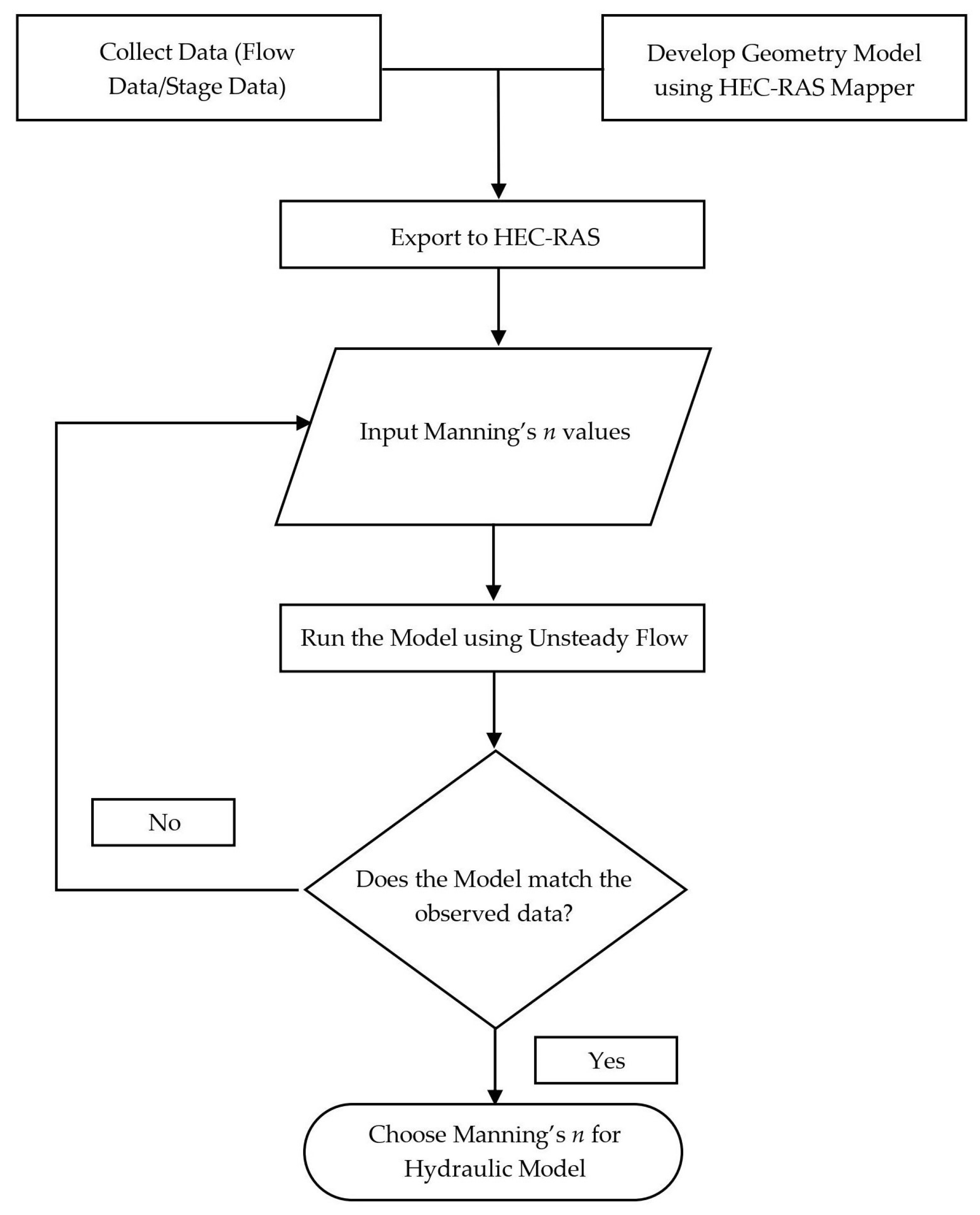
Figure 4.
Calibration of the flow model by iterating Manning’s n values.

Figure 5.
Simulation of the sediment model using the available transport functions.

Figure 6.
Total suspended solids in the Pasig River during (a) 25 February 2022 neap tide and (b) 3 March 2022 spring tide.
Figure 6.
Total suspended solids in the Pasig River during (a) 25 February 2022 neap tide and (b) 3 March 2022 spring tide.

Figure 7.
Calibration of water level in (m) during the dry season on (a) 25–26 February and (b) 1–2 March 2022.
Figure 7.
Calibration of water level in (m) during the dry season on (a) 25–26 February and (b) 1–2 March 2022.

Figure 8.
Coefficient of determination (R2) of (a) 25 February 2022, neap tide run and (b) 3 March 2022, spring tide run, using Copeland’s version of Laursen’s equation as Transport Function.
Figure 8.
Coefficient of determination (R2) of (a) 25 February 2022, neap tide run and (b) 3 March 2022, spring tide run, using Copeland’s version of Laursen’s equation as Transport Function.

Figure 9.
Simulated sediment concentration (mg/L) transported throughout the river.


Table 1.
Coordinates of the Pasig River Stations.
| Station | Latitude | Longitude | |
|---|---|---|---|
| 1 | Napindan (C6) Bridge | 14.5351 | 121.1022 |
| 2 | Bambang Bridge | 14.5536 | 121.0759 |
| 3 | Buayang Bato | 14.5683 | 121.0510 |
| 4 | Guadalupe Viejo | 14.5682 | 121.0410 |
| 5 | Lambingan Bridge | 14.5865 | 121.0198 |
| 6 | Nagtahan Bridge | 14.5959 | 121.0012 |
| 7 | Jones Bridge | 14.5958 | 120.9771 |
| 8 | Manila Bay | 14.5955 | 120.9618 |
Table 2.
Statistical analysis results for sediment concentration model calibration and validation.
| Statistical Index | Calibration 25 February 2022 | Validation | Optimal Value | |
|---|---|---|---|---|
| 25 February 2022 | 2 March 2022 | |||
| R2 | 0.9950 | 0.9989 | 0.9994 | 1 |
| d | 0.9983 | 0.9997 | 0.9998 | 1 |
| NSE | 0.9931 | 0.9986 | 0.9991 | 0.75–1 |
| PBIAS | 1.2915 | −0.4476 | −0.4607 | −15–0–15 |
| RSR | 0.0832 | 0.0369 | 0.0285 | 0.5–0 |
Table 3.
Statistic calibration of the model for sediment concentration (20 February 2020).
| Statistical Index | Calibration | Optimal Value |
|---|---|---|
| R2 | 0.9994 | 1 |
| d | 0.9999 | 1 |
| NSE | 0.99937 | 0.75–1 |
| PBIAS | −0.06997 | −15–0–15 |
| RSR | 0.02496 | 0.5–0 |
Disclaimer/Publisher’s Note: The statements, opinions and data contained in all publications are solely those of the individual author(s) and contributor(s) and not of MDPI and/or the editor(s). MDPI and/or the editor(s) disclaim responsibility for any injury to people or property resulting from any ideas, methods, instructions or products referred to in the content. |
© 2024 by the authors. Licensee MDPI, Basel, Switzerland. This article is an open access article distributed under the terms and conditions of the Creative Commons Attribution (CC BY) license (https://creativecommons.org/licenses/by/4.0/).
Share and Cite
MDPI and ACS Style
Casila, J.C.; Andres, H.L.; Haddout, S.; Yokoyama, K. Sediment Transport Modeling in the Pasig River, Philippines Post Taal Volcano Eruption. Geosciences 2024, 14, 45. https://0-doi-org.brum.beds.ac.uk/10.3390/geosciences14020045
AMA Style
Casila JC, Andres HL, Haddout S, Yokoyama K. Sediment Transport Modeling in the Pasig River, Philippines Post Taal Volcano Eruption. Geosciences. 2024; 14(2):45. https://0-doi-org.brum.beds.ac.uk/10.3390/geosciences14020045
Chicago/Turabian StyleCasila, Joan Cecilia, Howard Lee Andres, Soufiane Haddout, and Katsuhide Yokoyama. 2024. "Sediment Transport Modeling in the Pasig River, Philippines Post Taal Volcano Eruption" Geosciences 14, no. 2: 45. https://0-doi-org.brum.beds.ac.uk/10.3390/geosciences14020045
Note that from the first issue of 2016, this journal uses article numbers instead of page numbers. See further details here.